1. Introduction
Jet diffusion flames arise when a fuel is injected into an oxidizer, or vice versa, and ignited. Examples include flames in Bunsen burners with the air-hole closed (the yellow flame), rich-burn gas turbine combustion chambers, and liquid rocket engines. All jet diffusion flames are lifted to some extent, in the sense that the base of the flame sits downstream of the injection plane. This is because the fuel and oxidizer have to mix before they can support a flame that propagates upstream as fast as the flow moves downstream. In
 $\text{H}_{2}/\text{O}_{2}$
rocket engines, the flame speed is so high that the lift-off distance is a very small fraction of the flame diameter (Juniper & Candel Reference Juniper and Candel2003), typically of the order of the injector lip thickness. In Bunsen burners, on the other hand, the yellow flame is easily lifted by increasing the gas flow rate. The flame in a gas turbine combustion chamber differs because the inlet flow swirls, which creates a vortex breakdown bubble downstream of the injector in which hot gases recirculate, thereby anchoring the flame (Candel et al.
Reference Candel, Durox, Schuller, Bourqouin and Moeck2014). This flame, whether premixed, partially premixed, or non-premixed, is often lifted with a lift-off distance of around one jet diameter and, in this respect, is similar to a lifted jet diffusion flame.
There have been several studies of the hydrodynamic stability of reacting flows. Most have examined swirling premixed or partially premixed flames because of their relevance to gas turbines (Juniper Reference Juniper2012; Oberleithner, Schimek & Paschereit Reference Oberleithner, Schimek and Paschereit2015a
; Terhaar, Oberleithner & Paschereit Reference Terhaar, Oberleithner and Paschereit2015). These studies show that, in a non-reacting swirling flow, the helical mode with azimuthal wavenumber
 $m=1$
is usually absolutely unstable and that this causes the flow to have a precessing vortex core. These studies also show that the flame’s heat release changes the density and velocity fields, altering the hydrodynamic stability of the flow, in many cases suppressing the
 $m=1$
instability and hence the precessing vortex core. This concurs with experiments and large-eddy simulations (LES) of swirling premixed lifted flames (Giauque et al.
Reference Giauque, Selle, Gicquel, Poinsot, Buechner, Kaufmann and Wrebs2005; Roux et al.
Reference Roux, Lartigue, Poinsot, Meier and Berat2005; Boxx et al.
Reference Boxx, Arndt, Carter and Meier2012).
In this study, we examine non-swirling lifted jet diffusion flames because they are simpler than their swirling counterparts. In both swirling and non-swirling flames, the hydrodynamic stability of the flow upstream of the flame base differs considerably from that downstream of the flame base (Nichols, Chomaz & Schmid Reference Nichols, Chomaz and Schmid2009; Manoharan et al.
Reference Manoharan, Hansford, O’Connor and Hemchandra2015; Oberleithner et al.
Reference Oberleithner, Stohr, Seong, Arndt and Steinberg2015b
). In non-swirling lifted diffusion flames, the upstream region is more hydrodynamically unstable and, although short, can dominate the hydrodynamic instability of the entire flow. This has some practical importance because axisymmetric (
 $m=0$
) hydrodynamic instability in flames can couple with longitudinal thermo-acoustic oscillations and cause dangerous vibrations (Schadow & Gutmark Reference Schadow and Gutmark1992; Chakravarthy et al.
Reference Chakravarthy, Shreenivasan, Boehm, Dreizler and Janicka2007). However, this result does not necessarily carry over from non-swirling diffusion flames to swirling premixed flames. The principal questions in this study are the following. (i) Which part of the flow causes hydrodynamic oscillations? (ii) What mechanisms of hydrodynamic instability are active? (iii) What control measures, active or passive, could suppress these oscillations?
Nichols & Schmid (Reference Nichols and Schmid2008), referred to herein as NS08, carried out direct numerical simulations (DNS) of flames in non-buoyant low-density jets. By varying the Damköhler number,
 $\mathit{Da}$
, which represents the ratio of the rate of reaction to the rate of fluid convection, flames with different lift-off heights were obtained. Flames with sufficiently large lift-off heights were found to oscillate. For a range of Damköhler numbers, the axial location of the flame base was monitored over time and a fast Fourier transform (FFT) of this time trace was used to obtain spectra for flames with different mean lift-off heights. For the unstable flames, NS08 observed peaks at Strouhal numbers between
 $0.25<\mathit{St}<0.30$
and a peak between
 $0.0<\mathit{St}<0.05$
. Flames with smaller lift-off heights (higher
 $\mathit{Da}$
) exhibited less-sharp spectral peaks than flames with larger lift-off heights (lower
 $\mathit{Da}$
). Flames with sufficiently small lift-off heights did not oscillate. NS08 performed a local stability analysis around steady solutions for these lifted flames. They showed that the premixing region upstream of the flame base is locally absolutely unstable and that reducing the lift-off height shortens the region of absolute instability. Since the flame with the smallest lift-off height was found to be stable, they concluded that the velocity and density fields induced by the flame cannot support self-sustained oscillations and that the flame oscillations at
 $0.25<\mathit{St}<0.30$
must be caused by the absolutely unstable premixing zone.
In a subsequent study, referred to herein as NCS09, Nichols et al. (Reference Nichols, Chomaz and Schmid2009) accounted for the fact that the flame base imposes streamwise confinement on the jet in the premixing zone. They used a local stability analysis to show that this could lead to resonant modes with a higher growth rate than the absolute growth rate. Furthermore, they postulated that the nonlinear interaction between two or more resonant modes could cause the spectral peaks at
 $0<\mathit{St}<0.05$
observed in the nonlinear simulations.
So far, all stability analyses of jet diffusion flames have been local (Lingens et al. Reference Lingens, Neemann, Meyer and Schreiber1996; Nichols & Schmid Reference Nichols and Schmid2008; Manoharan et al. Reference Manoharan, Hansford, O’Connor and Hemchandra2015; Oberleithner et al. Reference Oberleithner, Stohr, Seong, Arndt and Steinberg2015b ). The heat release from the flame alters the hydrodynamic stability and causes the local stability properties to change abruptly. This violates one of the assumptions of local stability analysis: that the flow varies smoothly in the streamwise direction. In this study, therefore, we perform a global stability analysis of a lifted jet diffusion flame. The global analysis does not require the flow to vary smoothly. We then interpret these results with the aid of a local stability analysis. As in NS08 and NS09, the influence of buoyancy is not included. We use the direct and adjoint global modes to obtain the structural sensitivity (Giannetti & Luchini Reference Giannetti and Luchini2007) of the flow. This identifies the region where force–momentum feedback has most influence on the growth rate and frequency of global modes, and is often called the wavemaker region. One aim of this paper is to discover whether or not the oscillations observed in the nonlinear simulations of NC08 are caused by linear global instability. If so, we aim to identify the regions of space and physical mechanisms that are most influential in causing these oscillations, and particularly whether the low-frequency mode is indeed due to the interaction between two resonant modes. Another aim is to identify how the growth rates and frequencies of these modes may be controlled by altering the flow. For this, we use the framework developed by Hill (Reference Hill1992) and Marquet, Sipp & Jacquin (Reference Marquet, Sipp and Jacquin2008) to determine the effect of steady body forces on the growth rate and frequency of the global modes.
The flow is described in § 2. The stability analyses and their results at
 $\mathit{Da}=500\,000$
are described in § 3 for the global analysis and § 4 for the local analysis. The results at different Damköhler number are presented in § 5 and the sensitivity to a steady control force in § 6.
2. Flow configuration
We study the motion of an axisymmetric jet of fuel exiting into a large cylindrical domain, of length
 $X_{max}$
and radius
 $R_{max}$
, which is filled with oxidizer. The jet of fuel enters the domain at
 $x=0$
, and is aligned along the axis,
 $r=0$
. The fluid in the domain has velocity
 $\boldsymbol{u}=(u_{x},u_{r})$
, density
 ${\it\rho}$
, pressure
 $p$
, and temperature
 $T$
. The concentration of the fuel is described using the mixture fraction
 $Z$
, which has a value of
 $Z=1$
for pure fuel and
 $Z=0$
for pure oxidizer.
We follow the approach of NS08 and use the the reacting low-Mach-number (LMN) equations to describe the motion of the fluid. In non-dimensional form, these equations can be written as
 $$\begin{eqnarray}\displaystyle & \displaystyle \frac{\partial {\it\rho}}{\partial t}+\boldsymbol{{\rm\nabla}}\boldsymbol{\cdot }({\it\rho}\boldsymbol{u})=0, & \displaystyle\end{eqnarray}$$
 $$\begin{eqnarray}\displaystyle & \displaystyle \frac{\partial ({\it\rho}\boldsymbol{u})}{\partial t}=-\boldsymbol{{\rm\nabla}}p+\boldsymbol{{\rm\nabla}}\boldsymbol{\cdot }\left(\frac{1}{S_{1}\mathit{Re}}{\bf\tau}-{\it\rho}\boldsymbol{u}\boldsymbol{u}\right), & \displaystyle\end{eqnarray}$$
 $$\begin{eqnarray}\displaystyle & \displaystyle {\it\rho}\left(\frac{\partial Z}{\partial t}+\boldsymbol{u}\boldsymbol{\cdot }\boldsymbol{{\rm\nabla}}Z\right)=\frac{1}{S_{1}\,\mathit{Re}\,\mathit{Sc}}{\rm\nabla}^{2}Z, & \displaystyle\end{eqnarray}$$
 $$\begin{eqnarray}\displaystyle & \displaystyle {\it\rho}\left(\frac{\partial T}{\partial t}+\boldsymbol{u}\boldsymbol{\cdot }\boldsymbol{{\rm\nabla}}T\right)=\frac{1}{S_{1}\mathit{Re}\,\mathit{Pr}}{\rm\nabla}^{2}T+\mathit{Da}\,{\it\rho}^{3}{\it\omega}, & \displaystyle\end{eqnarray}$$
 $$\begin{eqnarray}\displaystyle & {\it\rho}[(S_{1}-1)Z+1][(S_{2}-1)T+1]=1, & \displaystyle\end{eqnarray}$$
 ${\bf\tau}=[\boldsymbol{{\rm\nabla}}\boldsymbol{u}+(\boldsymbol{{\rm\nabla}}\boldsymbol{u})^{\text{T}}]-(2/3)(\boldsymbol{{\rm\nabla}}\boldsymbol{\cdot }\unicode[STIX]{x1D66A})I$
is the non-isotropic component of the rate-of-strain tensor.
The flow variables have been non-dimensionalized by the jet diameter at inlet, jet axial velocity at inlet, and oxidizer density. The non-dimensional temperature is defined as
 $T=(T^{\ast }-T_{0})/(T_{f}-T_{0})$
, where
 $T^{\ast }$
(K) is the dimensional temperature,
 $T_{f}$
(K) is the dimensional adiabatic flame temperature, and
 $T_{0}$
is the dimensional ambient oxidizer temperature. The ratio of the oxidizer density to fuel density at the inlet defines the density ratio parameter,
 $S_{1}$
. The source term,
 $\mathit{Da}\,{\it\rho}^{3}{\it\omega}$
, is equivalent to the non-dimensional rate of enthalpy release per unit volume. For the rate of reaction,
 ${\it\omega}$
, we use a simple Arrhenius law that is identical to the one used by NS08:
 $$\begin{eqnarray}{\it\omega}=\left\{\left(Z-\frac{T}{s+1}\right)\left(1-Z-\frac{sT}{s+1}\right)-{\it\kappa}T^{2}\right\}\exp \!\left[\frac{-{\it\beta}(1-T)}{1-{\it\alpha}(1-T)}\right].\end{eqnarray}$$
The chemistry of the reaction is described by the mass stoichiometric ratio,
 $s$
, the equilibrium constant,
 ${\it\kappa}$
, the heat release parameter,
 ${\it\alpha}\equiv (T_{f}-T_{0})/T_{f}$
, and the Zeldovich number
 ${\it\beta}\equiv {\it\alpha}T_{a}/T_{f}$
, where
 $T_{a}$
(K) is the dimensional activation temperature of the reaction. The ratio of the adiabatic flame temperature to the oxidizer temperature at the inlet defines the temperature ratio parameter,
 $S_{2}\equiv T_{f}/T_{0}$
. The Reynolds number,
 $\mathit{Re}$
, is defined in terms of the jet diameter, jet axial velocity and fuel jet density. This definition introduces a
 $1/S_{1}$
factor in front of the viscous terms in (2.1). The Prandtl number,
 $\mathit{Pr}$
, and Schmidt number,
 $\mathit{Sc}$
, describe the ratio of the diffusivity of temperature and mass, respectively to the diffusivity of momentum.
In this study, we assume that the effects of buoyancy are negligible and that the viscosity and thermal diffusivity are uniform throughout the flow, and we set the non-dimensional parameters in (2.1) and (2.2) to the values used by NS08:
 $\mathit{Re}=1000$
,
 $S_{1}=7.0$
,
 $S_{2}=6.0$
,
 $\mathit{Pr}=\mathit{Sc}=0.7$
,
 $\mathit{Da}=5\times 10^{5}$
,
 $s=2$
,
 ${\it\kappa}=0.01,{\it\alpha}=0.833$
and
 ${\it\beta}=3$
. This choice of parameters produces flames that are thicker than those found in nature. This is acceptable because these flames are sufficiently thin in comparison to the wavelength of the hydrodynamic instabilities that are being investigated. This is particularly relevant if the wavemaker region is in the flame. In this case, it is important that the thickness of the flame relative to the thickness of the wavemaker region is checked a posteriori, which is done in § 3.2.
Equations (2.1a
–
e
) can be expressed in terms of the momentum,
 $\boldsymbol{m}\equiv {\it\rho}\boldsymbol{u}$
, temperature,
 $T$
, and mixture fraction,
 $Z$
, as
 $$\begin{eqnarray}\frac{\partial \boldsymbol{q}}{\partial t}=\mathscr{N}(\boldsymbol{q}),\end{eqnarray}$$
where
 $\boldsymbol{q}\equiv (m_{x},\,m_{r},\,Z,\,T)^{\text{T}}$
is the state vector and
 $\mathscr{N}(\cdot )$
is a nonlinear differential operator representing the action of the equations on the state vector. The density,
 ${\it\rho}$
, is not included in the state vector because it can be derived from
 $T$
and
 $Z$
. We use an axisymmetric version of the DNS code developed by NS08 to solve these equations. A fourth-order Runge–Kutta scheme is used to march the discretized equations forward in time. The equations are discretized in space using a sixth-order compact finite difference scheme. We use a grid with
 $511\times 1537$
points for a domain measuring
 $10.0\times 15.0$
jet diameters in the radial and axial directions respectively. This domain is longer than that used by NS08 and we find that it produces results that are sufficiently well-converged and well-resolved (table 1).
Domain size (
 $X_{max}$
,
 $R_{max}$
), number of grid points (
 $Sx$
,
 $Sr$
), and time-step (
 ${\rm\Delta}t$
) used in the simulations to check numerical convergence. The eigenvalues for modes A and B are shown. The real part represents the growth rate, and the imaginary part represents the frequency. Mesh M1 was used by NS08 and mesh M2 is used in this study.

Along the lateral boundary,
 $r=R_{max}$
, we use a viscous traction-free boundary condition for the momentum and set
 $T=0$
and
 $Z=0$
. At the outlet boundary,
 $x=X_{max}$
, we use a convective boundary condition for the momentum, temperature and mixture fraction. These boundary conditions model flow into a semi-infinite domain in the downstream and radial directions. The pressure-projection scheme used in the code uses a discrete cosine transform to set boundary conditions for the pressure at the inlet and outlet boundaries. For the base flow, we use a quarter-wave cosine transform, which sets
 $\text{d}p/\text{d}x=0$
at the inlet, and
 $p=0$
at the outlet boundary. Along the lateral boundary, we set
 $p=0$
. At the inlet, we impose the same velocity and mixture fraction profiles as those used by NS08. These top-hat profiles are formed from Michalke’s profile number two (Michalke Reference Michalke1984), with a shear-layer thickness parameter
 $D/2{\it\theta}_{0}=12.5$
. This signifies that the momentum thickness of the shear layer is 12.5 times smaller than the jet radius. We also add a small coflow of oxidizer surrounding the jet to improve numerical stability. The coflow velocity is 1 % of the jet velocity. We set the temperature profile at the inlet to be uniform and impose a Gaussian-shaped impulse at
 $(x,r)=(2.0,0.5)$
to ignite the fuel–oxidizer mixture in order to obtain the base flow.
We obtain a steady axisymmetric base flow,
 $\bar{\boldsymbol{q}}(x,r)$
, such that
 $\mathscr{N}(\bar{\boldsymbol{q}})=0$
, using selective frequency damping (SFD) (Akervik et al.
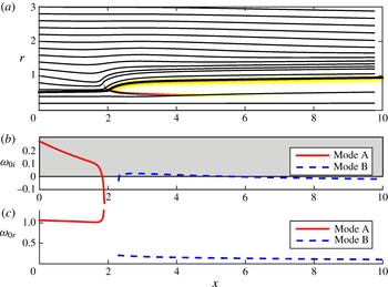
Reference Akervik, Brandt, Henningson, Hoepffner, Marxen and Schlatter2006). This base flow is shown in figure 1. The lift-off height,
 $H_{s}$
, matches that of the flame with
 $\mathit{Da}=500\,000$
in table 1 of NS08.
(a) The steady but unstable solution to the LMN equations for a lifted jet diffusion flame at
 $\mathit{Re}=1000$
and
 $\mathit{Da}=500\,000$
. The streamlines show the axial and radial velocity and the greyscale (colour online) shows contours of the reaction rate,
 $\log (\bar{{\it\omega}})$
. The azimuthal velocity is zero. The thick black line shows the stoichiometric surface, which corresponds to a contour of
 $\bar{Z}=0.333$
. (b) The absolute growth rate,
 ${\it\omega}_{0i}$
, as a function of axial position for the two modes that are absolutely unstable: mode A in the lifted region and mode B in the flame region. (c) The absolute frequency,
 ${\it\omega}_{0r}$
, of modes A and B.

3. Global stability
3.1. Numerical method
The evolution of small axisymmetric perturbations around this steady base flow is governed by the linearized reacting LMN equations. We decompose the axisymmetric perturbations into Fourier modes in time:
 $$\begin{eqnarray}\boldsymbol{q}^{\prime }(x,r,t)=\hat{\boldsymbol{q}}(x,r)\text{e}^{{\it\lambda}t}+\text{c.c.}\end{eqnarray}$$
The eigenvalue,
 ${\it\lambda}$
, contains the growth rate,
 $\text{Re}({\it\lambda})$
, and frequency,
 $\text{Im}({\it\lambda})$
, of the corresponding two-dimensional eigenmode,
 $\hat{\boldsymbol{q}}(x,r)$
, that would grow or decay on top of the steady base flow. The direct global modes are obtained by discretizing in space and solving the matrix eigenvalue problem
 $$\begin{eqnarray}{\it\lambda}\hat{\boldsymbol{q}}=\boldsymbol{L}\hat{\boldsymbol{q}},\end{eqnarray}$$
where
 $\boldsymbol{L}$
is a discretized operator that describes the linearized reacting LMN equations (given in appendix A). We also obtain the adjoint global modes, which are solutions of
 $$\begin{eqnarray}{\it\lambda}^{\ast }\hat{\boldsymbol{q}}^{+}=\boldsymbol{L}^{+}\hat{\boldsymbol{q}}^{+},\end{eqnarray}$$
where
 $\boldsymbol{L}^{+}$
is the discretized version of the continuous-adjoint reacting LMN equations (given in appendix A). We use the code developed by Chandler et al. (Reference Chandler, Juniper, Nichols and Schmid2012) to solve these eigenvalue problems using the same discretization as that used to obtain the base flow. The code uses matrix-free time-stepping of the linearized and adjoint reacting LMN equations, and the implicitly restarted Arnoldi method (Lehoucq, Sorensen & Yang Reference Lehoucq, Sorensen and Yang1998) to find the most unstable global modes. For the direct global modes, we use a convective boundary condition at the outlet boundary and set
 $\hat{m}_{x}=\hat{m}_{r}=\hat{T}=\hat{Z}=0$
on the lateral and inlet boundaries. For the adjoint global modes, we set
 $\hat{m}_{x}^{+}=\hat{m}_{r}^{+}=\hat{T}^{+}=\hat{Z}^{+}=0$
on all boundaries. For the linearized perturbations, we use a half-wave cosine transform to set the boundary conditions on the linearized pressure. This sets
 $\text{d}\hat{p}/\text{d}x=\text{d}\hat{p}^{+}/\text{d}x=0$
at the inlet and outlet boundaries. The adjoint global modes are normalized with respect to the corresponding direct global mode so that
 $$\begin{eqnarray}\langle \hat{\boldsymbol{m}}^{+},\hat{\boldsymbol{m}}\rangle +\langle \hat{Z}^{+},\hat{Z}\rangle +\langle \hat{T}^{+},\hat{T}\rangle =1.\end{eqnarray}$$
The notation
 $\langle \boldsymbol{a},\boldsymbol{b}\rangle$
denotes an inner product over the computational domain volume
 $V$
,
 $$\begin{eqnarray}\langle \boldsymbol{a},\boldsymbol{b}\rangle =\frac{1}{V}\int _{V}\boldsymbol{a}^{H}\boldsymbol{b}\;\text{d}V,\end{eqnarray}$$
where
 $\boldsymbol{a}^{H}$
denotes the Hermitian (i.e. complex-conjugate transpose) of
 $\boldsymbol{a}$
.
3.2. Direct and adjoint global modes
We look for the leading (least-stable or most-unstable) linear global modes for the flame with
 $\mathit{Da}=500\,000$
, shown in figure 1.
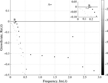
Figure 2 shows the leading eigenvalues with positive frequencies, together with the relative convergence of these eigenvalues. Amongst the modes that are well-converged, we find an isolated unstable high-frequency mode, and a branch of marginally stable low-frequency modes. There is a branch of stable low-frequency modes extending out from the origin. These modes are not well-converged and correspond to free-stream vortical modes. They arise from the continuous spectrum and are not considered in detail here. We consider the most-unstable mode and one of the marginally stable modes in more detail.
The least-stable part of the global eigenvalue spectrum for axisymmetric perturbations to the steady flow in figure 1. The greyscale indicates the relative convergence of these eigenvalues, as measured by the log of the Ritz estimates. The more negative the value (darker), the better the convergence.

The real component of the direct and adjoint global modes for mode A, which develops on the steady flow in figure 1. The eigenvalue is
 ${\it\lambda}=+0.157+1.365\text{i}$
(frequency 1.365, growth rate 0.157, Strouhal number 0.217): (a) direct global mode, (b) adjoint global mode.

The real component of the direct and adjoint global modes for mode B, which develops on the steady flow in figure 1. The eigenvalue is
 ${\it\lambda}=-0.005+0.170\text{i}$
(frequency 0.170, growth rate −0.005, Strouhal number 0.0271): (a) direct global mode, (b) adjoint global mode.

The first, labelled mode A, has an eigenvalue of
 ${\it\lambda}=+0.157+1.365\text{i}$
(frequency 1.365, growth rate 0.157,
 $\mathit{St}=0.217$
). The second, labelled mode B, has an eigenvalue of
 ${\it\lambda}=-0.005+0.170\text{i}$
(frequency 0.170, growth rate −0.005,
 $\mathit{St}=0.0271$
). The real components of the direct and adjoint global modes are shown in figure 3 for mode A and figure 4 for mode B. The structural sensitivity, as defined by Giannetti & Luchini (Reference Giannetti and Luchini2007) for the incompressible Navier–Stokes equations in the velocity–pressure formulation, is given by the dyadic product of the direct and adjoint global mode velocity vectors. For the LMN formulation used in this study, the equivalent quantity is the dyadic product of the direct and adjoint global mode momentum vectors,
 $\unicode[STIX]{x1D61A}_{ij}=\hat{\boldsymbol{m}}_{i}(\hat{\boldsymbol{m}}_{j}^{+})^{\ast }$
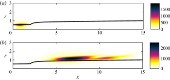
. The components of this tensor represent the effect of changes in the feedback between the different components of the perturbation momentum on the eigenvalue of the global mode. The Frobenius norms of this tensor for modes A and B are shown in figure 5. Where this quantity has a large magnitude, changes to the feedback mechanism that drives the instability have a large influence on the eigenvalue. Therefore, regions of high amplitude show the wavemaker region of the flow. The wavemaker regions are much longer than the thickness of the flame and are located on either side of the flame. This means that they are unaffected by the fact that the flame has been artificially thickened to aid numerical convergence, as described in § 1.
Contours of the Frobenius norm of the structural sensitivity tensor,
 $\unicode[STIX]{x1D61A}_{ij}=\hat{\boldsymbol{m}}_{i}(\hat{\boldsymbol{m}}_{j}^{+})^{\ast }$
, which is equivalent to (8.11) in Giannetti & Luchini (Reference Giannetti and Luchini2007). The high-amplitude (dark) regions show the wavemaker regions of the two modes. (a) Mode A, (b) mode B.

For mode A, the direct mode has highest amplitude just downstream of the flame base and grows radially towards the axis of the jet. The adjoint mode has highest amplitude in the premixing zone between the inlet and the flame base. The structural sensitivity, which is maximal at
 $(x,r)=(0.96,0.52)$
, shows that the wavemaker region for mode A lies in the shear layer in the premixing region upstream of the flame base.
For mode B, the direct mode has highest amplitude further downstream than for mode A. It lies along the outer part of the flame and grows radially away from the axis of the jet. The adjoint mode has high amplitude in the premixing zone and just downstream of the flame base. The structural sensitivity, which is maximal at
 $(x,r)=(6.73,1.13)$
, shows that the wavemaker region for mode B lies in the shear layer along the outer edge of the flame.
The Strouhal number for mode A is
 $\mathit{St}=0.217$
, which is close to the Strouhal number (
 $\mathit{St}=0.212$
) of the non-reacting jet in the nonlinear simulations of NS08 but 25 % less than the Strouhal number of the high-frequency mode observed at
 $\mathit{Da}=500\,000~(\mathit{St}=0.284)$
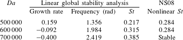
. The discrepancy could be due to the fact that the oscillations in the nonlinear simulations have appreciable amplitude and therefore their saturated frequency cannot be determined accurately from a linear analysis around the steady but unstable base flow. Nevertheless, these global stability results reinforce the conclusion of NS08 that the high-frequency mode is caused by the premixing region imparting its global instability frequency to the flame.
The Strouhal number for mode B is
 $\mathit{St}=0.0271$
, which is just 8 % more than that of the low-frequency mode observed in the nonlinear simulations of NS08 (
 $\mathit{St}=0.025$
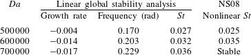
). Mode B is marginally stable (growth rate −0.005) and therefore acts as a lightly damped oscillator. This lightly damped oscillation can be observed in the transient behaviour of the nonlinear simulations shown in figure 3 of NS08. They did not perform a global stability analysis and therefore did not find mode B. It is likely that the low-frequency oscillation that they observe in their nonlinear simulation is caused by mode B, which is the flame region imparting its global instability frequency to the flame. NCS09 offer an alternative explanation: that the low-frequency oscillation is caused by interaction between two resonant modes. This is examined in § 4.3.
3.3. Components of the structural sensitivity
For variable-density and reacting flows, more information about the nature of the instability can be obtained by considering the structural sensitivity for the entire state vector and not just the momentum vector. For the flames in this section, this leads to a
 $4\times 4$
tensor, which represents the change in the eigenvalue due to changes in feedback from
 $m_{x}^{\prime }$
,
 $m_{r}^{\prime }$
,
 $Z^{\prime }$
and
 $T^{\prime }$
into the
 $x$
-momentum,
 $r$
-momentum, species, and energy equations. Comparison between sensitivities involving momentum, temperature and mixture fraction are valid as long as the adjoint global mode has been normalized according to (3.4), which is the case for the results presented here.
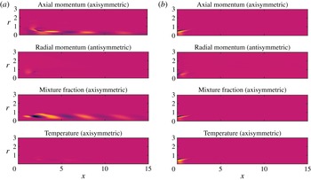
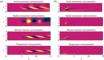
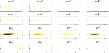
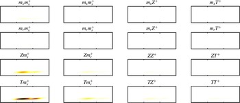
The sensitivity tensors for modes A and B are shown in figures 6 and 7 respectively. For mode A, the eigenvalue is most sensitive in the premixing region, particularly to changes in the feedback between the mixture fraction and the axial momentum equation. For mode B, the eigenvalue is most sensitive in the flame, particularly to changes in the feedback between the temperature and the axial momentum equation. The temperature and mixture fraction only affect the momentum equations indirectly, through the density. Therefore both these types of feedback mechanisms involve perturbations to the density. In the premixing region, which is at uniform temperature, these perturbations are caused mainly by perturbations to the mixture fraction. In the flame region, which has strong temperature gradients, these perturbations are caused mainly by perturbations to the temperature. This implies that the instability mechanism is the same for both modes.
The components of the structural sensitivity tensor
 $\hat{\boldsymbol{q}}(\hat{\boldsymbol{q}}^{+})^{\ast }$
for mode A. The shading on all the plots is equal and goes from 0 (white) to 11 470 (black). Each frame spans
 $0<x<2.5$
on the horizontal axis and
 $0<r<1.0$
on the vertical axis.

The components of the structural sensitivity tensor
 $\hat{\boldsymbol{q}}(\hat{\boldsymbol{q}}^{+})^{\ast }$
for mode B. The shading on all the plots is equal and goes from 0 (white) to 41 894 (black). Each frame spans
 $0<x<15.0$
on the horizontal axis and
 $0<r<5.0$
on the vertical axis.

4. Local stability analysis
The global analysis in § 3 reveals that there are two types of global modes, labelled A and B, with separate wavemaker regions. Comparing with the nonlinear simulations in NS08, mode A is reasonably close to the high-frequency oscillation and mode B matches the low-frequency oscillation. NCS09 suggested that the low-frequency oscillation could be caused by interaction between resonant modes in the lift-off region. In this section, we perform a local analysis in order to investigate this further.
4.1. Numerical method
For the local analysis (Huerre & Monkewitz Reference Huerre and Monkewitz1990) we use the linearized fully compressible Navier–Stokes equations with the Mach number set to 0.01. The WKBJ approximation is applied, in which the flow is considered to be locally parallel at each axial location. Wavy perturbations of the form
 $\exp [\text{i}(kx-{\it\omega}t)]$
are examined, in which
 $\text{Re}({\it\omega})$
is the frequency,
 $\text{Im}({\it\omega})$
is the temporal growth rate,
 $\text{Re}(k)$
is the wavenumber, and
 $\text{Im}(k)$
is the spatial growth rate. The governing equations, radial boundary conditions, and azimuthal wavenumber form a dispersion relation that is only satisfied for certain pairs of
 $(k,{\it\omega})$
. These are found numerically by discretizing the perturbations on Gauss–Lobatto-spaced points (G–L) in the radial direction, and solving the resulting generalized matrix eigenvalue problem. Saddle points of
 ${\it\omega}(k)$
are identified that satisfy (i) the dispersion relation, (ii)
 $\text{d}{\it\omega}/\text{d}k=0$
and (iii) the
 $k^{+}/k^{-}$
pinch point criterion. These waves have zero group velocity with absolute frequency,
 ${\it\omega}_{0}$
, and absolute wavenumber,
 $k_{0}$
. Further details of the method applied to an incompressible flow are in Juniper, Tammisola & Lundell (Reference Juniper, Tammisola and Lundell2011).
For the flow in figure 1, two dominant saddle points are found. Their absolute growth rates,
 ${\it\omega}_{0i}$
, and absolute frequencies,
 ${\it\omega}_{0r}$
, are shown as a function of axial location in figure 1(b,c). One saddle point exists in the premixing region and one in the flame region. We consider these regions separately.
4.2. Premixing region
In the premixing region, the flow is absolutely unstable (
 ${\it\omega}_{0i}>0$
) between the inlet plane and the flame base (
 $0<x<1.8$
). This distance is only 35 % of the absolute wavelength, which varies from 4.5 to 5.3 across the absolutely unstable region, and the streamwise boundaries to this region are abrupt. Consequently it is not accurate to estimate the complex frequency of the linear global mode either by finding a saddle point of
 ${\it\omega}_{0}(X)$
in the complex-
 $X$
-plane (Huerre & Monkewitz Reference Huerre and Monkewitz1990), or by taking the complex frequency of the most upstream location of absolute instability, as one would for a non-reacting hot jet (Monkewitz, Huerre & Chomaz Reference Monkewitz, Huerre and Chomaz1993). Instead, we perform a resonant mode calculation, as described by NCS09. This accounts for the abrupt boundary conditions in the streamwise direction. We perform this calculation on the flow at
 $X=0.0391$
because, based on the value of
 $k_{0}~(1.405-1.963\text{i})$
and
 ${\it\omega}_{0}~(1.062+0.2642\text{i})$
of the saddle point, this is the axial position of the results reported in NCS09. We also perform resonant mode calculations at other values of
 $X$
(not shown).
In the resonant mode calculation,
 $k^{+}$
and
 $k^{-}$
waves are found that satisfy the resonant condition
 $$\begin{eqnarray}\exp [\text{i}(k^{+}-k^{-})L]=\frac{1}{R^{+}R^{-}},\end{eqnarray}$$
where
 $R^{-}$
and
 $R^{+}$
are the reflection coefficients at the upstream and downstream boundaries. The reflection coefficients can either be set to −1 (perfect reflection) or, according to NCS09, can be calculated with
 $$\begin{eqnarray}R^{+}=-\frac{\displaystyle \int {\it\phi}^{+}(r)[{\it\phi}^{-}(r)]^{\dagger }r\,\text{d}r}{\displaystyle \int {\it\phi}^{+}(r)[{\it\phi}^{+}(r)]^{\dagger }r\,\text{d}r},\end{eqnarray}$$
where
 $\dagger$
denotes the adjoint. (The formula for
 $R^{-}$
has all the
 $+$
and
 $-$
superscripts reversed.) This accounts for imperfect overlap between the
 $k^{+}$
and
 $k^{-}$
waves at the boundaries, which leads to imperfect reflection.
In our calculations, points from
 $r=0$
to
 $\infty$
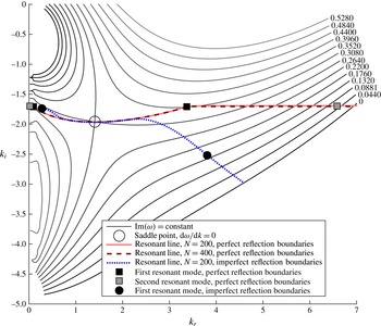
are mapped to G–L points from 0 to 1. Figure 8 shows contours of
 ${\it\omega}(k)$
around the saddle point for 200 G–L points, which is the resolution used by NCS09. As noted by NCS09 for this flow, and by Healey (Reference Healey2007) and Juniper (Reference Juniper2007) for similar flows, there are a set of poles along the
 $k_{i}$
axis, which are caused by the cross-stream confinement. These exist even when the outer point is mapped to infinity because the Dirichlet condition at
 $r=\infty$
is enforced by removing this point from the calculation, meaning that the penultimate point becomes the boundary.
Contours of
 ${\it\omega}_{i}(k)$
at
 $X=0.039$
for the
 $\mathit{Da}=500\,000$
flame shown in figure 1. Resonant lines are shown with both perfect reflection and imperfect reflection (4.2) at the boundaries. Resonant modes are shown for a flame lift-off height of
 $H_{s}=1.913$
, which is that of the
 $\mathit{Da}=500\,000$
flame. Comparison with figure 2 of Nichols et al. (Reference Nichols, Chomaz and Schmid2009) shows that the resonant modes are further apart in the
 $k$
-plane when this value value of
 $H_{s}$
is used.

Three resonant lines are shown for this model. The first is for
 $R^{+}=R^{-}=-1$
with 200 G–L points. This is identical to that in NCS09 but has been calculated to higher values of
 $k_{r}$
. The second is for
 $R^{+}=R^{-}=-1$
with 400 G–L points. These show that 200 G–L points are sufficient for convergence. The most unstable resonant mode has
 ${\it\omega}=1.329+0.2334\text{i}$
, (frequency 1.329, growth rate 0.2334,
 $\mathit{St}=0.2115$
) shown as a black square in figure 8. This is reasonably close to mode A from the global analysis (frequency 1.363, growth rate 0.159,
 $\mathit{St}=0.217$
). However, these resonant lines are affected by the presence of the saddle points along the
 $k_{i}$
axis, meaning that they are affected by the radial boundary condition, however far away it is (Juniper Reference Juniper2007). This dependence on the far-away radial boundary condition would be concerning but for the fact that, as the
 $k^{-}$
branch approaches the
 $k_{i}$
axis, the corresponding eigenfunction decays slowly in the
 $r$
direction and therefore has little overlap with that of the
 $k^{+}$
branch, which decays quickly in the
 $r$
direction. This means that the reflection coefficient is much less than 1 and (4.2) must be used instead. The third resonant line therefore is for
 $R^{+}$
and
 $R^{-}$
calculated with (4.2) with 200 G–L points. Based on this calculation, the most unstable resonant mode has
 ${\it\omega}=1.3352+0.15262\text{i}$
(frequency 1.3352, growth rate 0.15262,
 $\mathit{St}=0.2125$
). This is very close to mode A from the global analysis (frequency 1.363, growth rate 0.159,
 $\mathit{St}=0.217$
). In summary, mode A found from the global analysis seems to be a resonant mode in the premixing region, as proposed by NCS09.
4.3. Downstream of the flame base
NCS09 proposed that the low-frequency oscillations (
 $\mathit{St}=0.025$
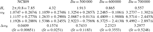
) observed in the nonlinear simulations in NS08 could be caused by interaction between resonant modes in the premixing region. They illustrate this by considering a premixing region that is 7.85 jet diameters long. Because it is long, it contains several unstable resonant modes with closely spaced frequencies, shown in the first column of table 2. The difference between the frequencies of the first two resonant modes is
 $0.0409~(\mathit{St}=0.00651)$
, which is around one-quarter that of the low-frequency oscillation. However, if the calculation is repeated with a premixing region that is 4.32 diameters long, shown in the second column of table 2, the difference between the first two resonant modes is exactly
 $0.1574~(\mathit{St}=0.0251)$
.
Flame lift-off height,
 $H_{s}$
, resonant modes,
 ${\it\omega}_{R}$
, (where
 $\text{Re}({\it\omega}_{R})$
is the frequency and
 $\text{Im}({\it\omega}_{R})$
is the growth rate), and the difference,
 ${\rm\Delta}{\it\omega}_{R}$
, between the frequencies of the first and second resonant modes expressed in rad s
 $^{-1}$
and as a Strouhal number. When
 $H_{s}=4.32$
,
 ${\rm\Delta}{\it\omega}_{R}$
matches the value of the low-frequency oscillations seen in NS08. However, when
 $H_{s}$
is set to the observed values,
 ${\rm\Delta}{\it\omega}_{R}$
is much higher and another explanation for the low-frequency oscillations is required.

The problem with this proposed mechanism is that the actual lift-off height at
 $\mathit{Da}=500\,000$
is much smaller than 4.32 jet diameters. The resonant modes calculated with the actual lift-off height, 1.913, are shown in the third column of table 2. The difference between the frequencies of the first two resonant modes is
 $0.7433~(\mathit{St}=0.1183)$
, which is 4.7 times greater than the low-frequency oscillations observed in the nonlinear simulations. Similar results are obtained when the resonant modes are calculated at all other streamwise locations in the premixing region, and for flames at
 $Da=600\,000$
and
 $Da=700\,000$
, as shown in the fourth and fifth columns of table 2. This shows that the low-frequency oscillations observed in the nonlinear simulations are not caused by interaction between resonant modes.
On the other hand, the local analysis in figure 1(b) shows that, downstream of the flame base, the flow is absolutely unstable due to the second saddle point. In this case, the absolutely unstable region does not encounter a rapid jump in the flow in the streamwise direction and it is appropriate to estimate the linear global mode growth rate by extending
 ${\it\omega}_{0}(X)$
into the complex-
 $X$
-plane and finding a saddle point. With this technique, the local analysis predicts the linear global mode to have
 ${\it\omega}_{g}=0.17324+0.014277\text{i}$
(frequency 0.17324, growth rate 0.014277,
 $\mathit{St}=0.02757$
). The local analysis is known to over-estimate the growth rate (Juniper et al.
Reference Juniper, Tammisola and Lundell2011), so this is sufficiently close to mode B (frequency 0.170, growth rate −0.004,
 $\mathit{St}=0.0271$
) to confirm that global mode B is caused by this region of absolute instability downstream of the flame base. Both are close to the observed frequency of
 $\mathit{St}=0.025$
. The local analysis therefore supports the conclusion of the global analysis: the low-frequency oscillations observed in the simulations of NS08 are caused by a linear global instability originating in the outer shear layer of the flame and not by the interaction between resonant modes.
5. Global modes at different Damköhler numbers
The global modes are calculated for two other values of the Damköhler number,
 $\mathit{Da}=600\,000$
and
 $\mathit{Da}=700\,000$
. The results are summarized in tables 3 and 4 and compared with the results of NS08. Near a supercritical Hopf bifurcation, the limit cycle amplitude increases in proportion to the square root of the linear growth rate. The linear growth rates for mode B decrease as
 $\mathit{Da}$
increases. If one assumes that nonlinear saturation mechanisms vary little with
 $\mathit{Da}$
then this concurs with the results in figure 3 of NS08, which show that the low-frequency spectral peak for
 $\mathit{Da}=600\,000$
is smaller than the low-frequency spectral peak for
 $\mathit{Da}=500\,000$
. The linear global mode frequencies for mode B agree well with those observed in the nonlinear simulations for
 $\mathit{Da}=500\,000$
and
 $\mathit{Da}=600\,000$
.
Comparison of growth rates and frequencies for mode A from a linear global stability analysis with frequencies from table 1 of NS08.

Comparison of growth rates and frequencies for mode B from a linear global stability analysis with the low-frequency oscillations observed in figure 3 of NS08.

6. Sensitivity to a control force
Having identified the two wavemaker regions and instability mechanisms active in the jet diffusion flame, we now consider how they could be controlled by perturbing the flow. We consider the effect of a small control force, which we model by adding source terms to the right-hand side of (2.3):
 $$\begin{eqnarray}\frac{\partial \boldsymbol{q}}{\partial t}=\mathscr{N}(\boldsymbol{q})+\boldsymbol{F},\end{eqnarray}$$
where
 $\boldsymbol{F}\equiv (\boldsymbol{f},0,\,{\it\psi}_{T})^{\text{T}}$
contains the source terms added to the right-hand side of the momentum, species and energy equations respectively. The source term in the species equation has been set to zero because this is unlikely to be a feasible method of control. The variables
 $\boldsymbol{f}$
and
 ${\it\psi}_{T}$
are the non-dimensional rates of addition per unit volume of momentum, and thermal energy into the flow. In this linear stability framework, the control force has a steady component,
 $\bar{\boldsymbol{F}}$
, which acts on the base flow,
 $\bar{\boldsymbol{q}}$
, and a linearized perturbation,
 $\boldsymbol{f}^{\prime }$
, which acts on the linear perturbations,
 $\boldsymbol{q}^{\prime }$
. We focus on the steady component of the control force because its effect is two orders of magnitude greater than the effect of the unsteady component of the control force.
The eigenvalue of the global mode,
 ${\it\lambda}$
, is a function of the base flow fields,
 $\bar{\boldsymbol{q}}$
, and these are, in turn, functions of the steady components of the forcing terms,
 $\bar{\boldsymbol{F}}$
. The effect of
 $\bar{\boldsymbol{F}}$
on
 ${\it\lambda}$
is calculated by formulating a constrained Lagrangian problem,
 $$\begin{eqnarray}\mathscr{L}={\it\lambda}-\langle \bar{\boldsymbol{q}}^{+},\mathscr{N}(\bar{\boldsymbol{q}})+\bar{\boldsymbol{F}}\rangle -\langle \hat{\boldsymbol{q}}^{+},{\it\lambda}\hat{\boldsymbol{q}}-\boldsymbol{L}\hat{\boldsymbol{q}}\rangle ,\end{eqnarray}$$
and calculating
 $\boldsymbol{{\rm\nabla}}_{\bar{\boldsymbol{F}}}{\it\lambda}$
, the functional derivative of
 ${\it\lambda}$
with respect to (w.r.t.)
 $\bar{\boldsymbol{F}}$
. This is labelled the sensitivity of the eigenvalue to steady forcing. The nonlinear and linearized reacting LMN equations act as constraints in this problem. The Lagrange multipliers,
 $\bar{\boldsymbol{q}}^{+}$
and
 $\hat{\boldsymbol{q}}^{+}$
, are the adjoint base flow and adjoint global mode fields respectively.
The sensitivity to steady forcing is equal to the functional derivative of
 $\mathscr{L}$
w.r.t.
 $\bar{\boldsymbol{F}}$
when all the constraints are satisfied. To find this, we first set the functional derivatives of
 $\mathscr{L}$
w.r.t. all other variables to zero. The derivative w.r.t.
 $\hat{\boldsymbol{q}}$
leads to a set of equations that defines the eigenvalue problem for the adjoint global mode,
 $-{\it\lambda}^{\ast }\hat{\boldsymbol{q}}^{+}+\boldsymbol{L}^{+}\hat{\boldsymbol{q}}^{+}=0$
. The derivative w.r.t.
 ${\it\lambda}$
leads to the normalization condition
 $\langle \hat{\boldsymbol{m}}^{+},\hat{\boldsymbol{m}}\rangle +\langle \hat{Z}^{+},\hat{Z}\rangle +\langle \hat{T}^{+},\hat{T}\rangle =1$
. The derivative w.r.t.
 $\bar{\boldsymbol{q}}$
leads to a set of equations (given in appendix A) for the adjoint base flow fields,
 $\bar{\boldsymbol{L}}^{+}\bar{\boldsymbol{q}}^{+}=\bar{\boldsymbol{g}}^{+}$
. The derivative w.r.t.
 $\bar{\boldsymbol{F}}$
then shows that the sensitivity of the eigenvalue to steady forcing is obtained from the relevant adjoint base flow field.
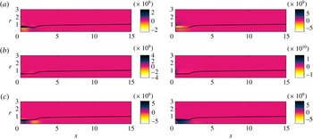
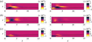
Figure 9 shows the sensitivity of mode A to steady body forces and a steady heat source. As for the low-density jet considered in Qadri (Reference Qadri2013), the sensitivity pattern for mode A of the lifted diffusion flame, in particular the sensitivity to axial forcing and heat input, roughly follows the streamline pattern in figure 1. The eigenvalue is most sensitive to a steady axial force on the lean side of the fuel–oxidizer shear layer upstream of the flame base. A radial force has most effect at the jet exit plane and at the flame base. Heating the core of the fuel jet upstream of the flame base is destabilizing. This is similar to the low-density jet. In general, the sensitive regions are concentrated around the jet shear layer and flame base. From a practical point of view, however, it would be difficult to apply control in these regions because the flame would tend to attach to the control device.
The sensitivity of the marginally stable eigenvalue of mode A for the lifted flame in figure 1 at
 $\mathit{Da}=500\,000$
, to steady forcing,
 $\boldsymbol{{\rm\nabla}}_{\bar{\boldsymbol{F}}}{\it\lambda}$
. The greyscale (colour online) shows the sensitivity of the growth rate (left), and frequency (right). (a) Sensitivity to a steady axial force, (b) sensitivity to a steady radial force, (c) sensitivity to steady heat input.

For mode B, on the other hand, regions of moderate to high sensitivity extend up to two jet diameters away from the jet axis and beyond. Passive control of this mode may, therefore, be a feasible option. A previous study by Toong et al. (Reference Toong, Salant, Stopford and Anderson1965) found that the flicker of a diffusion flame on a burning cylinder could be stabilized by placing a non-burning control cylinder on either side of the burning cylinder. From figure 10(a), it can be deduced that the drag force from a thin control ring has a strong effect on the eigenvalue: close to the flame it stabilizes mode B, while further from the flame, it destabilizes mode B. The drag force from a control ring also has an equivalently strong effect on the frequency of this mode: close to the flame, it increases the frequency, while further from the flame, it decreases the frequency. Toong et al. (Reference Toong, Salant, Stopford and Anderson1965) observed the frequency of oscillations to increase in their experiments.
As for figure 9 but for mode B: (a) sensitivity to a steady axial force, (b) sensitivity to a steady radial force, (c) sensitivity to steady heat input.

It is worth noting that the sensitivity to steady forcing for both modes of the lifted flame has a very large magnitude. This high sensitivity is caused by the linearization of the reaction rate around the base flow mixture fraction and temperature profiles. In particular, the eigenvalue is extremely sensitive to changes in the base flow mixture fraction profile. Physically, this means that a control device affects the growth rate and frequency of the global modes by affecting the base flow mixture fraction profile, which then affects the reaction rate. The high sensitivity also means that even a tiny perturbation will cause a large change in the base flow via this mechanism.
7. Conclusions
In this study, we have performed a linear global stability analysis of steady base flows for lifted diffusion flames with finite rate chemistry. We have considered a flow configuration that is identical to that considered by NS08. For each flame, we identify two types of axisymmetric modes that govern the instability dynamics. We have used their direct and adjoint global modes to identify the wavemaker responsible for each mode and to calculate the sensitivity of the growth rate and frequency of each mode to steady control forces. We have also applied local stability analysis in order to identify the instability mechanisms responsible for each mode.
The first of these modes, labelled mode A, has a linear global frequency close to the frequency of the high-frequency oscillations observed in the nonlinear simulations of NS08. The wavemaker for this mode is located in the shear layer in the premixing zone. The local analysis confirms the conclusions of NS08 and NCS09 that this mode is caused by a resonant mode in the lifted region upstream of the flame base. The components of the structural sensitivity tensor reveal that the eigenvalue is most sensitive to feedback of the perturbation density into the linearized axial momentum equations in the lifted region.
The second of these modes, labelled mode B, has a linear global frequency close to the frequency of the low-frequency oscillations observed in NS08. The wavemaker for this mode is located in the outer part of the shear layer in the flame. The local analysis shows that this is caused by a region of absolute instability in the flame, rather than by the nonlinear interaction of two resonant modes in the lifted region, which was the mechanism proposed by NCS09. The frequency that would arise from the nonlinear interaction of two resonant modes is several times larger than the frequency observed in the nonlinear simulations. The components of the sensitivity tensor reveal that the eigenvalue is most sensitive to the same feedback mechanism as that of mode A, but in the shear layer in the flame.
For mode A, the growth rate and frequency are most sensitive to steady forces applied near the jet shear layer upstream of the flame base. This suggests that passive control of this mode may not be feasible because the flame is likely to attach to any control devices placed at or near the flame base. For mode B, on the other hand, regions up to two or three diameters away from the fuel jet are moderately sensitive to steady forces. Passive control of this mode may, therefore, be feasible. The sensitivity map shows a large region where the drag force from a thin axisymmetric control ring can stabilize this mode of instability. This result tallies with Toong et al. (Reference Toong, Salant, Stopford and Anderson1965).
In this fundamental study, we have performed the first adjoint global stability analysis of a reacting flow, including the effects of finite rate chemistry. By using linear local and global stability analyses together, we have found that oscillations in lifted jet diffusion flames can be caused due to the interaction between different basic mechanisms of instability. The methods used here hold great promise for the use of linear stability analyses to study and control hydrodynamic instability in reacting flows, whether lifted or not.
Acknowledgement
This work was funded by the European Research Council through project ALORS 2590620.
Appendix A. Reacting LMN equation
A.1. Linearized LMN equations
 $$\begin{eqnarray}\displaystyle & \displaystyle \frac{\partial {\it\rho}^{\prime }}{\partial t}=-\boldsymbol{{\rm\nabla}}\boldsymbol{\cdot }\boldsymbol{m}^{\prime }, & \displaystyle\end{eqnarray}$$
 $$\begin{eqnarray}\displaystyle & \displaystyle \frac{\partial \boldsymbol{m}^{\prime }}{\partial t}=-\boldsymbol{{\rm\nabla}}p^{\prime }-\boldsymbol{{\rm\nabla}}\boldsymbol{\cdot }(\bar{{\it\rho}}\bar{\boldsymbol{u}}\boldsymbol{u}^{\prime }+\bar{{\it\rho}}\boldsymbol{u}^{\prime }\bar{\boldsymbol{u}}+{\it\rho}^{\prime }\bar{\boldsymbol{u}}\bar{\boldsymbol{u}})+\frac{1}{S_{1}\mathit{Re}}\,\boldsymbol{{\rm\nabla}}\boldsymbol{\cdot }{\bf\tau}^{\prime }, & \displaystyle\end{eqnarray}$$
 $$\begin{eqnarray}\displaystyle & \displaystyle \bar{{\it\rho}}\frac{\partial Z^{\prime }}{\partial t}=-\boldsymbol{m}^{\prime }\boldsymbol{\cdot }\boldsymbol{{\rm\nabla}}\bar{Z}-\bar{{\it\rho}}\bar{\boldsymbol{u}}\boldsymbol{\cdot }\boldsymbol{{\rm\nabla}}Z^{\prime }+\frac{1}{S_{1}\,\mathit{Re}\,\mathit{Sc}}{\rm\nabla}^{2}Z^{\prime }, & \displaystyle\end{eqnarray}$$
 $$\begin{eqnarray}\displaystyle & \displaystyle \bar{{\it\rho}}\frac{\partial T^{\prime }}{\partial t}=-\boldsymbol{m}^{\prime }\boldsymbol{\cdot }\boldsymbol{{\rm\nabla}}\bar{T}-\bar{{\it\rho}}\bar{\boldsymbol{u}}\boldsymbol{\cdot }\boldsymbol{{\rm\nabla}}T^{\prime }+\frac{1}{S_{1}\,\mathit{Re}\,\mathit{Pr}}{\rm\nabla}^{2}T^{\prime }+\mathit{Da}\,\bar{{\it\rho}}^{2}{\it\omega}^{\prime }, & \displaystyle\end{eqnarray}$$
 $$\begin{eqnarray}\displaystyle & \displaystyle \frac{{\it\rho}^{\prime }}{\bar{{\it\rho}}^{2}}=-\bar{K}_{1}T^{\prime }-\bar{K}_{2}Z^{\prime }, & \displaystyle\end{eqnarray}$$
 ${\bf\tau}^{\prime }\equiv [\boldsymbol{{\rm\nabla}}\boldsymbol{u}^{\prime }+(\boldsymbol{{\rm\nabla}}\boldsymbol{u}^{\prime })^{\text{T}}]-(2/3)(\boldsymbol{{\rm\nabla}}\boldsymbol{\cdot }\boldsymbol{u}^{\prime })\unicode[STIX]{x1D644}$
, the linearized momentum is
 $\boldsymbol{m}^{\prime }\equiv \bar{{\it\rho}}\boldsymbol{u}^{\prime }+{\it\rho}^{\prime }\bar{\boldsymbol{u}}$
, the linearized reaction rate is
 ${\it\omega}^{\prime }\equiv \bar{{\it\rho}}\bar{K}_{Z}Z^{\prime }+\bar{{\it\rho}}\bar{K}_{T}T^{\prime }+3{\it\rho}^{\prime }\bar{{\it\omega}}$
, and the additional scalar fields used for ease of reference are
 $$\begin{eqnarray}\displaystyle & \displaystyle \bar{K}_{1}\equiv (S_{2}-1)((S_{1}-1)\bar{Z}+1), & \displaystyle\end{eqnarray}$$
 $$\begin{eqnarray}\displaystyle & \displaystyle \bar{K}_{2}\equiv (S_{1}-1)((S_{2}-1)\bar{T}+1), & \displaystyle\end{eqnarray}$$
 $$\begin{eqnarray}\displaystyle & \displaystyle \bar{K}_{Z}\equiv \left(1-2\bar{Z}-\frac{s-1}{s+1}\bar{T}\right)\exp \left[\frac{-{\it\beta}(1-\bar{T})}{1-{\it\alpha}(1-\bar{T})}\right], & \displaystyle\end{eqnarray}$$
 $$\begin{eqnarray}\displaystyle \bar{K}_{T} & \equiv & \displaystyle \left\{\left[\left(\bar{Z}-\frac{\bar{T}}{s+1}\right)\left(1-\bar{Z}-\frac{s\bar{T}}{s+1}\right)-{\it\kappa}\bar{T}^{2}\right]\frac{{\it\beta}}{(1-{\it\alpha}(1-\bar{T}))^{2}}\right.\nonumber\\ \displaystyle & & \displaystyle \left.+\,2\bar{T}\left(\frac{s}{(s+1)^{2}}-{\it\kappa}\right)-\frac{1+(s-1)\bar{Z}}{s+1}\right\}\exp \left[\frac{-{\it\beta}(1-\bar{T})}{1-{\it\alpha}(1-\bar{T})}\right].\end{eqnarray}$$
A.2. Adjoint reacting LMN equations
 $$\begin{eqnarray}\displaystyle \frac{\partial \hat{m}_{i}^{+}}{\partial x_{i}}=0, & & \displaystyle\end{eqnarray}$$
 $$\begin{eqnarray}\displaystyle {\it\lambda}^{\ast }\hat{m}_{i}^{+} & = & \displaystyle \frac{\bar{m}_{j}}{\bar{{\it\rho}}}\left(\frac{\partial \hat{m}_{i}^{+}}{\partial x_{j}}+\frac{\partial \hat{m}_{j}^{+}}{\partial x_{i}}\right)+\frac{1}{\bar{{\it\rho}}}\frac{\partial \hat{p}^{+}}{\partial x_{i}}+\frac{1}{S_{1}\mathit{Re}\,\bar{{\it\rho}}}\left(\frac{\partial ^{2}\hat{m}_{i}^{+}}{\partial x_{j}^{2}}+\frac{1}{3}\frac{\partial ^{2}\hat{m}_{j}^{+}}{\partial x_{j}\partial x_{i}}\right)\nonumber\\ \displaystyle & & \displaystyle -\,\frac{\hat{T}^{+}}{\bar{{\it\rho}}}\frac{\partial \bar{T}}{\partial x_{i}}-\frac{\hat{Z}^{+}}{\bar{{\it\rho}}}\frac{\partial \bar{Z}}{\partial x_{i}},\end{eqnarray}$$
 $$\begin{eqnarray}\displaystyle {\it\lambda}^{\ast }\hat{Z}^{+} & = & \displaystyle \bar{m}_{i}\frac{\partial }{\partial x_{i}}\left(\frac{\hat{Z}^{+}}{\bar{{\it\rho}}}+\bar{K}_{2}\hat{p}^{+}\right)+\frac{1}{S_{1}\,\mathit{Re}\,\mathit{Sc}}\frac{\partial ^{2}}{\partial x_{i}^{2}}\left(\frac{\hat{Z}^{+}}{\bar{{\it\rho}}}+\bar{K}_{2}\hat{p}^{+}\right)\nonumber\\ \displaystyle & & \displaystyle +\,\mathit{Da}\,\bar{{\it\rho}}^{3}\left(\frac{\hat{T}^{+}}{\bar{{\it\rho}}}+\bar{K}_{1}\hat{p}^{+}\right)(\bar{K}_{Z}-3\bar{K}_{2}\bar{{\it\rho}}\bar{{\it\omega}})-\bar{K}_{2}\hat{{\it\rho}}^{+},\end{eqnarray}$$
 $$\begin{eqnarray}\displaystyle {\it\lambda}^{\ast }\hat{T}^{+} & = & \displaystyle \bar{m}_{i}\frac{\partial }{\partial x_{i}}\left(\frac{\hat{T}^{+}}{\bar{{\it\rho}}}+\bar{K}_{1}\hat{p}^{+}\right)+\frac{1}{S_{1}\mathit{Re}\,\mathit{Pr}}\frac{\partial ^{2}}{\partial x_{i}^{2}}\left(\frac{\hat{T}^{+}}{\bar{{\it\rho}}}+\bar{K}_{1}\hat{p}^{+}\right)\nonumber\\ \displaystyle & & \displaystyle +\,\mathit{Da}\,\bar{{\it\rho}}^{3}\left(\frac{\hat{T}^{+}}{\bar{{\it\rho}}}+\bar{K}_{1}\hat{p}^{+}\right)(\bar{K}_{T}-3\bar{K}_{1}\bar{{\it\rho}}\bar{{\it\omega}})-\bar{K}_{1}\hat{{\it\rho}}^{+},\end{eqnarray}$$
 $$\begin{eqnarray}\displaystyle \hat{{\it\rho}}^{+} & = & \displaystyle -\bar{m}_{i}\bar{m}_{j}\frac{\partial \hat{m}_{i}^{+}}{\partial x_{j}}-\frac{\bar{m}_{i}}{S_{1}\,\mathit{Re}}\left(\frac{\partial ^{2}\hat{m}_{i}^{+}}{\partial x_{j}^{2}}+\frac{1}{3}\frac{\partial ^{2}\hat{m}_{j}^{+}}{\partial x_{j}\partial x_{i}}\right).\end{eqnarray}$$
A.3. Sensitivity to steady forcing
The sensitivity to steady forcing is obtained from the adjoint base flow, which is defined by the equations
 $$\begin{eqnarray}\frac{\partial \bar{m}_{i}^{+}}{\partial x_{i}}=0,\end{eqnarray}$$
 $$\begin{eqnarray}\displaystyle & \displaystyle -\frac{\bar{m}_{j}}{\bar{{\it\rho}}}\left(\frac{\partial \bar{m}_{i}^{+}}{\partial x_{j}}-\frac{\partial \bar{m}_{j}^{+}}{\partial x_{i}}\right)-\frac{\partial \bar{p}^{+}}{\partial x_{i}}-\frac{1}{S_{1}\mathit{Re}\,\bar{{\it\rho}}}\left(\frac{\partial ^{2}\bar{m}_{i}^{+}}{\partial x_{j}^{2}}+\frac{1}{3}\frac{\partial ^{2}\bar{m}_{j}^{+}}{\partial x_{j}\partial x_{i}}\right)+\bar{T}^{+}\frac{\partial \bar{T}}{\partial x_{i}}+\bar{Z}^{+}\frac{\partial \bar{Z}}{\partial x_{i}}=\bar{f}_{i}^{+}, & \displaystyle \nonumber\\ \displaystyle & & \displaystyle\end{eqnarray}$$
 $$\begin{eqnarray}\displaystyle & \displaystyle -\bar{m}_{i}\frac{\partial \bar{Z}^{+}}{\partial x_{i}}-\frac{1}{S_{1}\,\mathit{Re}\,\mathit{Sc}}\frac{\partial ^{2}\bar{Z}^{+}}{\partial x_{i}^{2}}-\mathit{Da}\,\bar{{\it\rho}}^{3}\bar{T}^{+}(\bar{K}_{Z}-3\bar{K}_{2}\bar{{\it\rho}}\bar{{\it\omega}})+\bar{K}_{2}\bar{{\it\rho}}\bar{{\it\rho}}^{+}=\bar{{\it\psi}}_{Z}, & \displaystyle\end{eqnarray}$$
 $$\begin{eqnarray}\displaystyle & \displaystyle -\bar{m}_{i}\frac{\partial \bar{T}^{+}}{\partial x_{i}}-\frac{1}{S_{1}\mathit{Re}\,\mathit{Pr}}\frac{\partial ^{2}\bar{T}^{+}}{\partial x_{i}^{2}}-\mathit{Da}\,\bar{{\it\rho}}^{3}\bar{T}^{+}(\bar{K}_{T}-3\bar{K}_{1}\bar{{\it\rho}}\bar{{\it\omega}})+\bar{K}_{1}\bar{{\it\rho}}\bar{{\it\rho}}^{+}=\bar{{\it\psi}}_{T}, & \displaystyle\end{eqnarray}$$
 $$\begin{eqnarray}\displaystyle & \displaystyle \frac{\bar{m}_{i}\bar{m}_{j}}{\bar{{\it\rho}}^{2}}\frac{\partial \bar{m}_{i}^{+}}{\partial x_{j}}+\frac{\bar{m}_{i}}{S_{1}\,\mathit{Re}\,\bar{{\it\rho}}^{2}}\left(\frac{\partial ^{2}\bar{m}_{i}^{+}}{\partial x_{j}^{2}}+\frac{1}{3}\frac{\partial ^{2}\bar{m}_{j}^{+}}{\partial x_{j}\partial x_{i}}\right)+\frac{\bar{{\it\rho}}^{+}}{\bar{{\it\rho}}}=\bar{{\it\varrho}}^{+}. & \displaystyle\end{eqnarray}$$
 $\bar{\boldsymbol{g}}^{+}\equiv (\,\bar{f}_{i}^{+},\bar{{\it\psi}}_{Z}^{+},\bar{{\it\psi}}_{T}^{+})^{T}$
and
 $\bar{{\it\varrho}}^{+}$
represent the sensitivity of the eigenvalue to local base flow modifications and are given by
 $$\begin{eqnarray}\displaystyle \bar{f_{i}}^{+} & \equiv & \displaystyle \left(\frac{\hat{m}_{j}^{\ast }}{\bar{{\it\rho}}}-\frac{\hat{{\it\rho}}^{\ast }\bar{m}_{j}}{\bar{{\it\rho}}^{2}}\right)\left(\frac{\partial \hat{m}_{i}^{+}}{\partial x_{j}}+\frac{\partial \hat{m}_{j}^{+}}{\partial x_{i}}\right)-\frac{\hat{{\it\rho}}^{\ast }}{S_{1}\mathit{Re}\bar{{\it\rho}}^{2}}\left(\frac{\partial ^{2}\hat{m}_{i}^{+}}{\partial x_{j}^{2}}+\frac{1}{3}\frac{\partial ^{2}\hat{m}_{j}^{+}}{\partial x_{j}\partial x_{i}}\right)\nonumber\\ \displaystyle & & \displaystyle -\,\left(\frac{\hat{T}^{+}}{\bar{{\it\rho}}}+\bar{K}_{1}\hat{p}^{+}\right)\frac{\partial \hat{T}^{\ast }}{\partial x_{i}}-\left(\frac{\hat{Z}^{+}}{\bar{{\it\rho}}}+\bar{K}_{2}\hat{p}^{+}\right)\frac{\partial \hat{Z}^{\ast }}{\partial x_{i}},\end{eqnarray}$$
 $$\begin{eqnarray}\displaystyle \bar{{\it\psi}}_{Z}^{+} & \equiv & \displaystyle \frac{\partial }{\partial x_{j}}\left(\frac{\hat{Z}^{+}\hat{m}_{j}^{\ast }}{\bar{{\it\rho}}}\right)-(S_{2}-1)(S_{1}-1)\hat{p}^{+}\left(\bar{m}_{j}\frac{\partial \hat{T}^{\ast }}{\partial x_{j}}-\frac{1}{S_{1}\,\mathit{Re}\,\mathit{Pr}}\frac{\partial ^{2}\hat{T}^{\ast }}{\partial x_{j}^{2}}\right)\nonumber\\ \displaystyle & & \displaystyle -\,(S_{2}-1)(S_{1}-1)\hat{{\it\rho}}^{+}\hat{T}^{\ast }+\mathit{Da}\,\bar{{\it\rho}}^{2}\hat{p}^{+}[\bar{{\it\rho}}(\bar{K}_{1}{\it\delta}\bar{K}_{Z,{\it\delta}Z}+(S_{2}-1)(S_{1}-1)\bar{K}_{Z})\hat{Z}^{\ast }\nonumber\\ \displaystyle & & \displaystyle +\,\bar{{\it\rho}}(\bar{K}_{1}{\it\delta}\bar{K}_{T,{\it\delta}Z}+(S_{2}-1)(S_{1}-1)\bar{K}_{T})\hat{T}^{\ast }-3\bar{{\it\rho}}^{2}((\bar{K}_{1}^{2}\bar{K}_{Z}+2(S_{2}-1)\nonumber\\ \displaystyle & & \displaystyle \times \,(S_{1}-1)\bar{K}_{1}\bar{{\it\omega}})\hat{T}^{\ast }+(\bar{K}_{1}\bar{K}_{2}\bar{K}_{Z}+(S_{2}-1)(S_{1}-1)\bar{K}_{2}\bar{{\it\omega}})\hat{Z}^{\ast })]\nonumber\\ \displaystyle & & \displaystyle +\,\mathit{Da}\,\bar{{\it\rho}}^{2}({\it\delta}\bar{K}_{Z,{\it\delta}Z}\hat{Z}^{\ast }+{\it\delta}\bar{K}_{T,{\it\delta}Z}\hat{T}^{\ast })\hat{T}^{+}-3\,\mathit{Da}\,\bar{{\it\rho}}^{3}\hat{T}^{+}\nonumber\\ \displaystyle & & \displaystyle \times \,((\bar{K}_{1}\bar{K}_{Z}+(S_{2}-1)(S_{1}-1)\bar{{\it\omega}})\hat{T}^{\ast }+\bar{K}_{2}\bar{K}_{Z}\hat{Z}^{\ast }),\end{eqnarray}$$
 $$\begin{eqnarray}\displaystyle \bar{{\it\psi}}_{T}^{+} & \equiv & \displaystyle \frac{\partial }{\partial x_{j}}\left(\frac{\hat{T}^{+}\hat{m}_{j}^{\ast }}{\bar{{\it\rho}}}\right)-(S_{2}-1)(S_{1}-1)\hat{p}^{+}\left(\bar{m}_{j}\frac{\partial \hat{Z}^{\ast }}{\partial x_{j}}-\frac{1}{S_{1}\,\mathit{Re}\,\mathit{Sc}}\frac{\partial ^{2}\hat{Z}^{\ast }}{\partial x_{j}^{2}}\right)\nonumber\\ \displaystyle & & \displaystyle -\,(S_{2}-1)(S_{1}-1)\hat{{\it\rho}}^{+}\hat{Z}^{\ast }+\mathit{Da}\,\bar{{\it\rho}}^{2}\hat{p}^{+}[\bar{{\it\rho}}\bar{K}_{1}{\it\delta}\bar{K}_{Z,{\it\delta}T}\hat{Z}^{\ast }+\bar{{\it\rho}}\bar{K}_{1}{\it\delta}\bar{K}_{T,{\it\delta}T}\hat{T}^{\ast }\nonumber\\ \displaystyle & & \displaystyle -\,3\bar{{\it\rho}}^{2}(\bar{K}_{1}^{2}\bar{K}_{T}\hat{T}^{\ast }+(\bar{K}_{1}\bar{K}_{2}\bar{K}_{T}+(S_{2}-1)(S_{1}-1)\bar{K}_{1}\bar{{\it\omega}})\hat{Z}^{\ast })]\nonumber\\ \displaystyle & & \displaystyle +\,\mathit{Da}\,\bar{{\it\rho}}^{2}({\it\delta}\bar{K}_{Z,{\it\delta}T}\hat{Z}^{\ast }+{\it\delta}\bar{K}_{T,{\it\delta}T}\hat{T}^{\ast })\hat{T}^{+}\nonumber\\ \displaystyle & & \displaystyle -\,3\,\mathit{Da}\,\bar{{\it\rho}}^{3}\hat{T}^{+}((\bar{K}_{2}\bar{K}_{T}+(S_{2}-1)(S_{1}-1)\bar{{\it\omega}})\hat{Z}^{\ast }+\bar{K}_{1}\bar{K}_{T}\hat{T}^{\ast }),\end{eqnarray}$$
 $$\begin{eqnarray}\displaystyle \bar{{\it\varrho}}^{+} & \equiv & \displaystyle 2\frac{\hat{{\it\rho}}^{\ast }\hat{{\it\rho}}^{+}}{\bar{{\it\rho}}^{3}}-\frac{\hat{m}_{j}^{\ast }}{\bar{{\it\rho}}^{2}}\frac{\partial \hat{p}^{+}}{\partial x_{j}}+\frac{\hat{T}^{+}}{\bar{{\it\rho}}^{2}}\left(\bar{m}_{j}\frac{\partial \hat{T}^{\ast }}{\partial x_{j}}+\hat{m}_{j}^{\ast }\frac{\partial \bar{T}}{\partial x_{j}}\right)+\frac{\hat{Z}^{+}}{\bar{{\it\rho}}^{2}}\left(\bar{m}_{j}\frac{\partial \hat{Z}^{\ast }}{\partial x_{j}}+\hat{m}_{j}^{\ast }\frac{\partial \bar{Z}}{\partial x_{j}}\right)\nonumber\\ \displaystyle & & \displaystyle -\,\frac{\hat{T}^{+}}{S_{1}\mathit{Re}Pr\bar{{\it\rho}}^{2}}\frac{\partial ^{2}\hat{T}^{\ast }}{\partial x_{j}^{2}}-\frac{\hat{Z}^{+}}{S_{1}\mathit{Re}Pr\bar{{\it\rho}}^{2}}\frac{\partial ^{2}\hat{Z}^{\ast }}{\partial x_{j}^{2}}-\left(\frac{\bar{m}_{i}\hat{m}_{j}^{\ast }}{\bar{{\it\rho}}^{2}}+\frac{\hat{m}_{i}^{\ast }\bar{m}_{j}}{\bar{{\it\rho}}^{2}}-\frac{2\hat{{\it\rho}}^{\ast }\bar{m}_{i}\bar{m}_{j}}{\bar{{\it\rho}}^{3}}\right)\nonumber\\ \displaystyle & & \displaystyle \times \,\frac{\partial \hat{m}_{i}^{+}}{\partial x_{j}}-\frac{1}{S_{1}\mathit{Re}}\left(\frac{\hat{m}_{j}^{\ast }}{\bar{{\it\rho}}^{2}}-\frac{\hat{{\it\rho}}^{\ast }\bar{m}_{j}}{\bar{{\it\rho}}^{3}}\right)\left(\frac{\partial ^{2}\hat{m}_{i}^{+}}{\partial x_{j}^{2}}+\frac{1}{3}\frac{\partial ^{2}\hat{m}_{j}^{+}}{\partial x_{j}\partial x_{i}}\right)\nonumber\\ \displaystyle & & \displaystyle +\,3\,\mathit{Da}\,\bar{{\it\rho}}^{2}\bar{K}_{1}\hat{p}^{+}(\bar{K}_{Z}\hat{Z}^{\ast }+\bar{K}_{T}\hat{T}^{\ast })+2\,\mathit{Da}\,\bar{{\it\rho}}\hat{T}^{+}(\bar{K}_{Z}\hat{Z}^{\ast }+\bar{K}_{T}\hat{T}^{\ast })\nonumber\\ \displaystyle & & \displaystyle -\,12\,\mathit{Da}\,\bar{{\it\rho}}^{3}\bar{{\it\omega}}\bar{K}_{1}\hat{p}^{+}(\bar{K}_{1}\hat{T}^{\ast }+\bar{K}_{2}\hat{Z}^{\ast })-9\,\mathit{Da}\,\bar{{\it\rho}}^{2}\bar{{\it\omega}}\hat{T}^{+}(\bar{K}_{1}\hat{T}^{\ast }+\bar{K}_{2}\hat{Z}^{\ast }).\end{eqnarray}$$
The additional scalar fields introduced by linearizing the expressions in (A 4) and (A 5) around
 $\bar{Z}$
and
 $\bar{T}$
are given by
 $$\begin{eqnarray}\displaystyle {\it\delta}\bar{K}_{Z,{\it\delta}Z}\equiv -2\exp \left[\frac{-{\it\beta}(1-\bar{T})}{1-{\it\alpha}(1-\bar{T})}\right], & & \displaystyle\end{eqnarray}$$
 $$\begin{eqnarray}\displaystyle {\it\delta}\bar{K}_{Z,{\it\delta}T} & = & \displaystyle {\it\delta}\bar{K}_{T,{\it\delta}Z}\equiv \left[\left(1-2\bar{Z}-\frac{s-1}{s+1}\bar{T}\right)\frac{{\it\beta}}{(1-{\it\alpha}(1-\bar{T}))^{2}}-\frac{s-1}{s+1}\right]\nonumber\\ \displaystyle & & \displaystyle \times \,\exp \left[\frac{-{\it\beta}(1-\bar{T})}{1-{\it\alpha}(1-\bar{T})}\right],\end{eqnarray}$$
 $$\begin{eqnarray}\displaystyle {\it\delta}\bar{K}_{T,{\it\delta}T} & \equiv & \displaystyle \left\{\left[\left(-\frac{1}{s+1}\left(1-\bar{Z}-\frac{s\bar{T}}{s+1}\right)-\frac{s}{s+1}\left(\bar{Z}-\frac{\bar{T}}{s+1}\right)-2{\it\kappa}\bar{T}\right)\right.\right.\nonumber\\ \displaystyle & & \displaystyle \left.\left.-\,\frac{2{\it\alpha}}{1-{\it\alpha}(1-\bar{T})}\left(\left(\bar{Z}-\frac{\bar{T}}{s+1}\right)\left(1-\bar{Z}-\frac{s\bar{T}}{s+1}\right)-{\it\kappa}\bar{T}^{2}\right)\right.\right.\nonumber\\ \displaystyle & & \displaystyle \left.\left.+\,\frac{{\it\beta}}{(1-{\it\alpha}(1-\bar{T}))^{2}}\left(\left(\bar{Z}-\frac{\bar{T}}{s+1}\right)\left(1-\bar{Z}-\frac{s\bar{T}}{s+1}\right)-{\it\kappa}\bar{T}^{2}\right)\right.\right.\nonumber\\ \displaystyle & & \displaystyle \left.\left.+\,\left(2\bar{T}\left(\frac{s}{(s+1)^{2}}-{\it\kappa}\right)-\frac{1+(s-1)\bar{Z}}{s+1}\right)\right]\frac{{\it\beta}}{(1-{\it\alpha}(1-\bar{T}))^{2}}\right.\nonumber\\ \displaystyle & & \displaystyle \left.+\,2\left(\frac{s}{(s+1)^{2}}-{\it\kappa}\right)\right\}\exp \left[\frac{-{\it\beta}(1-\bar{T})}{1-{\it\alpha}(1-\bar{T})}\right].\end{eqnarray}$$