



1. Introduction
Shallow-water models are widely utilised in both geophysical and astrophysical fluid dynamics. By assuming much larger horizontal length scales than the vertical scale, these models effectively capture the essential dynamics of large-scale motions in the ocean, atmosphere and astrophysical flows. This paper focuses on the equatorial shallow-water system on a
 $\beta$
-plane, where the Coriolis force varies linearly with latitude. Near the equator, the rotation serves as a waveguide, confining waves to the equatorial region. These waves are known as equatorial shallow-water waves.
The linear dynamics of equatorial shallow-water waves was first studied by Matsuno (Reference Matsuno1966), who derived dispersion relations for various wave types. Using terminology introduced later (e.g. Majda et al. Reference Majda, Rosales, Tabak and Turner1999; Pedlosky Reference Pedlosky2013), these waves are classified as Kelvin, Poincaré, Rossby and Yanai waves. Their dispersion relations are illustrated in figure 1. Kelvin waves have a constant phase velocity that is independent of wavelength and propagate eastward. Poincaré waves, also known as inertio-gravity waves, exhibit high phase velocities and can propagate both eastward and westward. Rossby waves, which are influenced by the
 $\beta$
-effect, propagate westward. These waves are analogous to those in more familiar contexts, such as shallow water on an
 $f$
-plane or two-dimensional flow on a
 $\beta$
-plane. Yanai waves, also referred to as mixed Rossby–gravity waves, have dispersion curves that connect Rossby waves and eastward-propagating Poincaré waves. Matsuno’s theory has been validated by numerous observations in both the ocean and the atmosphere (e.g. Yanai & Maruyama Reference Yanai and Maruyama1966; Wallace & Kousky Reference Wallace and Kousky1968; see Kiladis et al. Reference Kiladis, Wheeler, Haertel, Straub and Roundy2009 for a review).
Equatorial shallow-water waves play a crucial role in significant climate phenomena such as El Niño and the Madden–Julian Oscillation (MJO). During El Niño, the temperature initially increases in the western Pacific. Eastward-propagating Kelvin waves then transport this heat to the eastern Pacific, leading to a temperature rise (Straub, Kiladis & Ciesielski Reference Straub, Kiladis and Ciesielski2006; Fedorov & Brown Reference Fedorov and Brown2009). The MJO refers to variations in tropical precipitation, driven by a coherent structure of varying moisture that moves eastward through the atmosphere. A recent theory suggests that these coherent structures can be understood as ‘modons’, which are pairs of moving vortices in equatorial shallow water. The dynamics of modons are closely related to nonlinear Rossby waves (Yano & Tribia Reference Yano and Tribia2017; Rostami & Zeitlin Reference Rostami and Zeitlin2019a , Reference Rostami and Zeitlinb ). Recent studies have demonstrated that more realistic shallow-water models, which incorporate moisture convection, can predict modons that capture essential features of the MJO (Rostami & Zeitlin Reference Rostami and Zeitlin2020; Rostami, Zhao & Petri Reference Rostami, Zhao and Petri2022; Cao et al. Reference Cao, Kurganov, Liu, Rostami and Zeitlin2025).
Dispersion relations of linear equatorial shallow-water waves. The wavenumber
 $k$
and frequency
 $\omega$
have been rescaled by
 $\beta ^{ {1}/{2}}(gH)^{- {1}/{4}}$
and
 $\beta ^{ {1}/{2}}(gH)^{ {1}/{4}}$
, respectively, where
 $\beta$
represents the gradient of the Coriolis parameter,
 $g$
is the acceleration due to gravity and
 $H$
denotes the mean depth of the fluid layer.

Figure 1. Long description
A line graph illustrating the dispersion relations of linear equatorial shallow-water waves. The x-axis represents the wavenumber, rescaled by the gradient of the Coriolis parameter, ranging from -5 to 5. The y-axis represents the frequency, rescaled by the acceleration due to gravity and the mean depth of the fluid layer, ranging from 0 to 6. The graph features multiple curves labeled as Poincaré, Kelvin, Yanai, and Rossby waves. The Poincaré waves are represented by multiple curves that form a parabolic shape, opening upwards. The Kelvin wave is depicted by a single curve that starts at the origin and increases linearly. The Yanai wave is shown by a curve that starts at the origin and increases non-linearly. The Rossby wave is represented by a curve that starts at the origin and increases slowly. All values are approximated.
A notable characteristic of the shallow-water model is the tendency to form shocks. A shock is a discontinuity in either velocity or surface height and is significant in geophysics. In oceanic contexts, a shock may signal wave overturning or indicate hydraulic jumps, both of which can lead to wave breaking (Fedorov & Melville Reference Fedorov and Melville1995, Reference Fedorov and Melville2000). The mechanism behind shock formation is now well understood. The shallow-water equations, when rotation is not considered, are equivalent to those governing compressible gases, which are known for their ability to produce shocks (Whitham Reference Whitham1974; Lighthill Reference Lighthill1978). When rotation is included – either in coastal shallow water on an
 $f$
-plane (Bennett Reference Bennett1973; Fedorov & Melville Reference Fedorov and Melville1995) or in equatorial shallow water on a
 $\beta$
-plane (Boyd Reference Boyd1980; Ripa Reference Ripa1982) – Kelvin waves can develop into shocks. The non-dispersive nature of Kelvin waves is crucial in this nonlinear evolution, as there is no dispersive mechanism for energy radiation. Meanwhile, nonlinear advection terms dominate as wave amplitudes increase, causing wavefronts to steepen. Additionally, studies show that shock formation can be effectively approximated using the Burgers equation (Burgers Reference Burgers1948).
Numerical simulations of the evolution of Kelvin waves in the equatorial shallow-water system have been conducted by Fedorov & Melville (Reference Fedorov and Melville2000), Le Sommer, Reznik & Zeitlin (Reference Le Sommer, Reznik and Zeitlin2004) and Bouchut, Le Sommer & Zeitlin (Reference Bouchut, Le Sommer and Zeitlin2005). Their findings confirm that Kelvin waves evolve into shocks, showing qualitative agreements with the theories proposed by Boyd (Reference Boyd1980) and Ripa (Reference Ripa1982). However, the simulation results indicate that the shocks exhibit complex profiles with very small-scale structures, which are not captured by the simple jump predicted by the Burgers equation. Fedorov & Melville (Reference Fedorov and Melville2000) provided an insightful explanation for this phenomenon. They revealed that the complex shock profile arises from the first Poincaré wave excited by the Kelvin wave. Additionally, they proposed a mechanism for this excitation: nonlinearity causes the Kelvin wave to travel faster, allowing it to catch up with the Poincaré wave and achieve resonance.
In this paper, we conduct a theoretical study of the dynamic behaviours of equatorial shallow-water waves, focusing particularly on the role of Poincaré waves. While Fedorov & Melville (Reference Fedorov and Melville2000) primarily explored these waves through direct numerical simulations, our objective is to develop a reduced model that enhances our understanding of the nonlinear dynamics of both the Kelvin wave and the first Poincaré wave, offering deeper physical insights. Our analysis demonstrates that the velocity of the Kelvin wave does not need to precisely match that of the Poincaré wave for the latter to be generated. Notably, excitation can occur even with a slight difference in their phase velocities. Additionally, our model is computationally efficient, enabling ultrahigh resolutions that allow us to uncover the detailed structure of shocks.
A central topic of this study is the effects of dispersion introduced by Poincaré waves. The impact of dispersion in linear waves is well understood; however, its effects in nonlinear waves are significantly more complex, especially concerning shocks. In the Korteweg–de Vries (KdV) and nonlinear Schrödinger (NLS) equations, it has been shown that dispersion smooths the discontinuities of shock waves and results in high-frequency quasi-periodic oscillations (see e.g. El & Hoefer Reference El and Hoefer2016; Carretero-Gonzalez, Frantzeskakis & Kevrekidis Reference Carretero-Gonzalez, Frantzeskakis and Kevrekidis2024). In geophysical fluid dynamics, nonlinear one-dimensional Poincaré waves can be modelled using the Ostrovsky equation (Ostrovsky Reference Ostrovsky1978). A further simplified version of the Ostrovsky equation, which considers rotation as the sole source of dispersion, is known as the reduced Ostrovsky equation or the Hunter–Ostrovsky equation. Research has shown that while the dispersion weakens the shocks, waves with sufficiently large amplitudes or short wavelengths can still produce shocks (Hunter Reference Hunter1990; Boyd Reference Boyd2005a ; Grimshaw, Helfrich & Johnson Reference Grimshaw, Helfrich and Johnson2012).
In the absence of dispersion, Wang, Wang & Hajduk (Reference Wang, Wang and Hajduk2020) investigated the nonlinear interaction between the Kelvin wave and the first Poincaré wave. They examined a scenario involving significantly short waves, where the phase velocities of both waves are identical. Their theory predicts that the Poincaré wave exhibits a simple jump at the shock, similar to that of the Kelvin wave. However, results from direct numerical simulations reveal more complex shock structures, which they suggest may arise from dispersion.
The remainder of the paper is organised as follows. In § 2, we present the governing equations for the equatorial shallow-water system. In § 3, we conduct a theoretical analysis to derive a reduced model for the dynamics of the Kelvin wave and the first Poincaré wave. We summarise the model in § 4, solve it numerically and use the solutions to investigate the dynamics of dispersive shocks. In § 5, we perform numerical simulations on the equatorial shallow-water equations and compare the results with our theoretical predictions. Finally, we draw our conclusions in § 6.
2. Governing equations
The mechanism and properties of equatorial waves can be illustrated by considering horizontally propagating waves in a rotating fluid of uniform finite depth
 $H$
, where
 $H$
is small compared with the horizontal extent of the fluid. The fluid is assumed to have a homogeneous density and a free surface. This idealised representation is referred to in geophysical fluid dynamics as a shallow-water model. Specifically, we consider equatorial shallow-water flow on a
 $\beta$
-plane, where the Coriolis parameter is
 $ f=\beta y$
, with
 $y$
denoting latitude and
 $x$
denoting longitude. Let the velocities in the
 $(x,y)$
directions be represented as
 $(u,v)$
, and the surface deformation as
 $\eta$
; then, the governing equations of the system read
 \begin{align} u_t+uu_x+vu_y-\beta yv&=-g\eta _x, \end{align}
 \begin{align} v_t+uv_x+vv_y+\beta yu&=-g\eta _y, \end{align}
 \begin{align} \eta _t+\left [u(H+\eta )\right ]_x+\left [v(H+\eta )\right ]_y&=0, \end{align}
where the subscripts denote partial differentiation. By using
 \begin{equation} L=\beta ^{- 1/2}(gH)^{1/4},\quad T=\beta ^{- 1/2}(gH)^{- 1/4},\quad \frac {L}{T},\quad H \end{equation}
to rescale
 $(x,y)$
,
 $t$
,
 $(u,v)$
and
 $\eta$
, we can derive the corresponding non-dimensional equations:
 \begin{align} u_t+uu_x+vu_y-yv&=-\eta _x, \end{align}
 \begin{align} v_t+uv_x+vv_y+yu&=-\eta _y, \end{align}
 \begin{align} \eta _t+\left [u(1+\eta )\right ]_x+\left [v(1+\eta )\right ]_y&=0. \end{align}
We consider periodic boundary conditions in the
 $x$
direction, while
 $(u,v,\eta )\rightarrow 0$
as
 $y\rightarrow \pm \infty$
. The equations in system (2.3) are the primitive dimensionless equations for equatorial shallow-water waves. In § 3, we perform a theoretical analysis of these equations and derive a reduced model for the nonlinear dynamics of the Kelvin wave and the first Poincaré wave. Readers who prefer not to delve into details of the mathematical derivation can skip ahead to § 4.1, where we summarise the model. Additionally, we numerically solve system (2.3) in § 5 to validate our theoretical findings.
3. A theoretical analysis
In this section, we conduct a theoretical analysis of equatorial shallow-water waves. Our analytical progress involves asymptotic analysis at small amplitudes and short wavelengths. In § 3.1, we undertake a linear analysis, from which we demonstrate potential resonance between waves. Then, in § 3.2, we derive the evolution equations for the nonlinear waves.
3.1. Linear analysis
Linear shallow-water equatorial waves have been studied by Matsuno (Reference Matsuno1966), who has given the complete spectrum. Here, the focus is on short Yanai and Poincaré waves with phase velocities close to those of Kelvin waves. In particular, we derive a linear wave equation with a dispersive term, providing a foundation to build the nonlinear wave equations.
To study the linear waves, we omit the product terms in (2.3) considering small wave amplitudes, and obtain the linearised equations:
 \begin{equation} u_t-yv+\eta _x=0,\quad v_t+yu+\eta _y=0,\quad \eta _t+u_x+v_y=0. \end{equation}
To address the
 $y$
dependence, a common approach is to assume normal modes in both
 $x$
and
 $t$
, such as
 $u=\hat {u}(y){\rm e}^{{\rm i}(kx-\omega t)}$
, and then solve the ordinary differential equations in
 $y$
to derive the dispersion relation. However, in the present problem, our main objective is to derive simplified wave equations, so we take a different approach: we retain the dependence on
 $x$
and
 $t$
while expanding the variables in terms of their eigenfunctions in
 $y$
. Boyd (Reference Boyd1980) introduced an effective technique for this approach, which we will adopt.
Boyd (Reference Boyd1980) suggested that the derivation can be significantly simplified by considering the sum and difference of
 $\eta$
and
 $u$
:
 \begin{equation} S=\eta +u,\qquad D=\eta -u. \end{equation}
The equations for
 $S$
and
 $D$
are given by
 \begin{align} S_t+S_x+\left (\frac {\partial }{\partial y}-y\right )v&=0, \end{align}
 \begin{align} v_t+\frac {1}{2}\left (\frac {\partial }{\partial y}+y\right )S+\frac {1}{2}\left (\frac {\partial }{\partial y}-y\right )D&=0, \end{align}
 \begin{align} D_t-D_x+\left (\frac {\partial }{\partial y}+y\right )v_x&=0. \end{align}
Both
 $S$
and
 $D$
can be expressed in terms of their eigenfunctions in
 $y$
, based on the linear theory proposed by Matsuno (Reference Matsuno1966):
 \begin{equation} \left (S,v,D\right )={\rm e}^{- {y^2}/{2}}\sum _{n=0}^\infty \left [S_n(x,t),v_n(x,t),D_n(x,t)\right ]\frac {H_n(y)}{2^n}, \end{equation}
where
 $H_n$
represents the
 $n$
th-order Hermite polynomial. For convenience, we list the first five Hermite polynomials:
 \begin{equation} \begin{aligned} &H_0=1,\qquad H_1=2y,\qquad H_2=4y^2-2,\\ &H_3=8y^3-12y,\qquad H_4=16y^4-48y^2+12. \end{aligned} \end{equation}
Boyd (Reference Boyd1980) noted that the differential operators in (3.3) correspond to those found in the recurrence relations of the eigenfunctions:
 \begin{align} &\left (\frac {\partial }{\partial y}-y\right )\left [H_n(y){\rm e}^{- {y^2}/{2}}\right ]=-H_{n+1}(y){\rm e}^{- {y^2}/{2}}, \end{align}
 \begin{align} &\left (\frac {\partial }{\partial y}+y\right )\left [H_n(y){\rm e}^{- {y^2}/{2}}\right ]=2nH_{n-1}(y) {\rm e}^{- {y^2}/{2}}. \\[10pt] \nonumber \end{align}
This relation enables us to easily derive the equations for each order of expression (3.4). Specifically, for
 $n=0$
, we have
 \begin{equation} S_{0,t}+S_{0,x}=0\,; \end{equation}
for
 $n=1$
,
 \begin{equation} S_{1,t}+S_{1,x}-v_0=0,\quad v_{0,t}+ S_1=0\,; \end{equation}
and for
 $n\ge 2$
,
 \begin{align} S_{n,t}+S_{n,x}-v_{n-1}&=0, \end{align}
 \begin{align} v_{n-1,t}+nS_{n}-\frac {1}{2}D_{n-2}&=0, \end{align}
 \begin{align} D_{n-2,t}-D_{n-2,x}+2(n-1)v_{n-1}&=0. \end{align}
Equations (3.7) and (3.8) describe the dynamics of Kelvin waves and Yanai waves, respectively, and system (3.9) incorporates Rossby waves and Poincaré waves. By applying the normal mode form proportional to
 ${\rm e}^{{\rm i}(kx-\omega t)}$
, the non-trivial conditions from (3.7)–(3.9) yield the dispersion relations. For
 $n=0$
, (3.7) gives the frequency of the Kelvin wave:
 \begin{equation} \omega =k. \end{equation}
For
 $n=1$
, system (3.8) gives the dispersion relation for the Yanai wave:
 \begin{equation} \omega -k-\frac {1}{\omega }=0. \end{equation}
For
 $n\ge 2$
, system (3.9) results in the dispersion relation for Poincaré and Rossby waves:
 \begin{equation} \omega ^2-k^2-\frac {k}{\omega }=2n-1. \end{equation}
Numerical solutions of these dispersion relations are plotted in figure 1. Various types of resonance are possible among linear equatorial shallow-water waves, leading to nonlinear interactions among different modes. For a comprehensive overview of triad interactions and resonance involving wave packets, the interested reader is referred to Ripa (Reference Ripa1983a
,Reference Ripa
b
) and Boyd (Reference Boyd1983). In the present study, we concentrate on the resonance of Kelvin waves within a continuous spectrum. The Kelvin wave is non-dispersive, meaning its phase velocity (
 $\omega /k=1$
) is constant. As a result, waves of differing wavelengths can resonate and produce nonlinear evolution (Boyd Reference Boyd1980; Ripa Reference Ripa1982).
Short Yanai and Poincaré waves may resonate with Kelvin waves due to their similar phase velocities. Their dispersion relations (3.11) and (3.12) indicate that as
 $k\rightarrow \infty$
, one of the limits of
 $\omega /k$
is unity, which corresponds to the phase velocity of the Kelvin wave. The interaction of these three types of waves in this limit has been investigated by Wang et al. (Reference Wang, Wang and Hajduk2020). In the current study, we focus on the scenario where
 $k$
is large but finite. For instance, figure 1 shows that at approximately
 $k=5$
, the phase velocities of the Yanai and Poincaré waves differ only slightly from those of the Kelvin wave. We therefore examine the large-
 $k$
behaviour of (3.8) and (3.9). Assuming that the waves are characterised by
 ${\rm e}^{{\rm i}k(x-ct)}$
, where
 $k$
is large and
 $c$
is close to unity, (3.9c
) indicates that, at leading order,
 \begin{equation} D_{n-2,t}-D_{n-2,x}= 2D_{n-2,t}=-2(n-1)\,v_{n-1}. \end{equation}
It then follows that
 \begin{equation} D_{n-2}=-(n-1)\int v_{n-1}\,{\rm d}t= v_{n-1}\times O\bigl(k^{-1}\bigr), \end{equation}
suggesting that
 $D_{n-2}$
is much smaller than
 $v_{n-1}$
. Next, we consider (3.9b
). By comparing the orders of
 $v_{n-1,t}$
and
 $D_{n-2}$
, one can demonstrate using (3.14) that
 \begin{equation} v_{n-1,t}=v_{n-1}\times O(k),\qquad -\frac {1}{2}D_{n-2}=v_{n-1}\times O\bigl(k^{-1}\bigr). \end{equation}
This suggests that, in the limit of large
 $k$
,
 $v_{n-1,t}$
is significantly larger than
 $D_{n-2}$
in (3.9b
). Therefore, we can neglect the latter and derive
 \begin{equation} v_{n-1}=-n\int S_n\,{\rm d}t. \end{equation}
Equation (3.16) shows that
 $S_n$
is of the order of
 $k$
larger than
 $v_{n-1}$
, making it
 $O(k^2)$
larger than
 $D_{n-2}$
according to (3.14). Consequently, we can disregard the difference between
 $\eta$
and
 $u$
for large wavenumbers. If we define
 $\eta _n$
and
 $u_n$
similarly to (3.4), we find that
 \begin{equation} u_n=\eta _n=\frac {S_n}{2}\equiv A_n. \end{equation}
Substituting (3.16) and (3.17) into (3.9a ) results in the evolution equation:
 \begin{equation} A_{n,t}+A_{n,x}+n\int A_n\,{\rm d}t=0. \end{equation}
We can verify that this holds for
 $n=0$
and
 $n=1$
in (3.7) and (3.8) as well.
Equation (3.18) describes the linear evolution of Kelvin, Yanai and Poincaré waves at large wavenumbers. The leading order of this equation is
 $A_{n,t}+A_{n,x}=0$
, which represents non-dispersive transport, and the integral term accounts for dispersion at the next order. This is more clearly illustrated by examining the dispersion relation of (3.18):
 \begin{equation} \omega -k-\frac {n}{\omega }=0, \end{equation}
where the term
 $-n/\omega$
indicates weak dispersion at large wavenumber
 $k$
. Additionally, it can be verified that (3.19) is consistent with (3.10) and (3.11), and it represents the large-
 $k$
limit of (3.12). To illustrate the role of dispersion in wave modulation, we can examine the dependence on the variables
 \begin{equation} \theta =k(x-t)\quad \text{and}\quad \tau =\delta t, \end{equation}
where
 $\theta$
represents the phase of the non-dispersive part of the wave and
 $\tau$
, with
 $\delta \ll 1$
, reflects slow wave modulation. The leading-order modulation equation is then given by
 \begin{equation} A_{n,\tau }-\frac {n}{k\delta }\int A_{n}\,{\rm d}\theta =0, \end{equation}
which shows that modulation is driven by the integral dispersive term. Note that the integral term is no longer small if
 $\delta =O(k^{-1})$
, but we will specify
 $\delta$
through nonlinear analysis, where nonlinearity decides the time scale of wave modulation. Additionally, it is worth noting that (3.21) consists of
 $O(\delta )$
terms of (3.18), suggesting that even weak nonlinearity can contribute to modulation, which we explore next.
3.2. The nonlinear analysis
Having identified the potential resonance between linear waves, we set out to investigate the resulting nonlinear dynamics. We limit our attention to the nonlinear evolution of an initially linear Kelvin wave, which is responsible for shock formation, and leave the study of other initial conditions for future research. At an early stage, the wave field is given by
 \begin{equation} u=\eta =\varepsilon {\rm e}^{- {y^2}/{2}}\sin (kx-kt),\quad v=0, \quad \text{for}\quad t\ll 1, \end{equation}
where
 $\varepsilon$
is a small parameter representing the order of the wave amplitude. In our linear analysis, we demonstrated that short Poincaré waves have phase velocities close to that of the Kelvin wave and can therefore be excited by the latter. We restrict our nonlinear analysis to the dynamics of the Kelvin wave and the first Poincaré wave. The Yanai wave is excluded on the grounds of symmetry: since both the initial Kelvin wave and the newly excited Poincaré waves are even in
 $y$
, they have zero projection onto the odd eigenspace of the Yanai wave. Furthermore, previous numerical simulations (Fedorov & Melville Reference Fedorov and Melville2000) suggest that the first Poincaré wave dominates the response during Kelvin wave evolution, while higher-order modes remain negligible. This is consistent with our analysis, which indicates that the initial Kelvin wave exerts only weak forcing on these higher-order modes. Consequently, we neglect higher-order Poincaré waves and assume that the dynamics is primarily governed by the first mode. We acknowledge that we do not have a rigorous justification for this assumption; its validity will be assessed a posteriori through comparison with numerical simulations.
There are two scenarios for this excitation of the first Poincaré wave. The first scenario begins with a short Kelvin wave, meaning that the wavenumber
 $k$
is large. This wave then excites short Poincaré waves through a resonance mechanism. The second scenario starts with a long linear Kelvin wave, which cannot directly excite Poincaré waves. However, this Kelvin wave evolves into a shock that has a small length scale, where the Poincaré waves are excited locally. In the following, we analyse the first scenario and derive a reduced model for the nonlinear wave dynamics. We have found that the same reduced model is also applicable to the second scenario, which we briefly discuss at the end of this section.
We again adopt the variables
 $S$
and
 $D$
as defined in (3.2), but now retain the nonlinear terms in the primitive (2.3). These equations may be rearranged to yield
 \begin{align} S_t+S_x+\left (\frac {\partial }{\partial y}-y\right )v=-uu_x-(u\eta )_x-vu_y-(v\eta )_y&\equiv F, \end{align}
 \begin{align} v_t+\frac 12\left (\frac {\partial }{\partial y}+y\right )S+\frac 12\left (\frac {\partial }{\partial y}-y\right )D=-uv_x-vv_y&\equiv E, \end{align}
 \begin{align} D_t-D_x+\left (\frac {\partial }{\partial y}+y\right )v_x=uu_x-(u\eta )_x+vu_y-(v\eta )_y&\equiv G. \end{align}
The nonlinear terms are defined as
 $F$
,
 $E$
and
 $G$
, and we expand them by the eigenfunctions of linear waves as in (3.4):
 \begin{equation} \begin{aligned} (F,E,G)={\rm e}^{- {y^2}/{2}}\sum _{n=0}^\infty \left [F_n(x,t),E_n(x,t),G_n(x,t)\right ]\frac {H_n(y)}{2^n}. \end{aligned} \end{equation}
The projection onto each eigenfunction is calculated by exploiting the completeness and orthogonality of the Hermite polynomials; for instance, the coefficients are given by
 \begin{equation} F_n=\frac {\displaystyle \int _{-\infty }^\infty FH_n(y){\rm e}^{- {y^2}/{2}}\,{\rm d}y}{\sqrt {\pi }n!}, \end{equation}
with analogous expressions for
 $E_n$
and
 $G_n$
. Substituting (3.4) and (3.24) into (3.23) and isolating the
 $n=0$
and
 $n=2$
components, which correspond to the Kelvin wave and the first Poincaré wave, respectively, we arrive at the governing equations. Given that the linear terms are identical to those in (3.7) and (3.9), this procedure yields
 \begin{equation} S_{0,t}+S_{0,x}=F_0 \end{equation}
and
 \begin{align} S_{2,t}+S_{2,x}-v_{1}&=F_2, \end{align}
 \begin{align} v_{1,t}+2S_2-\frac {1}{2}D_{0}&=E_1, \end{align}
 \begin{align} D_{0,t}-D_{0,x}+2v_1&=G_{0}. \end{align}
The initial condition derived from (3.22) is given by
 \begin{equation} S_0=2\varepsilon \sin (kx-kt),\quad S_2=v_1=D_0=0,\quad t\rightarrow 0, \end{equation}
signifying a pure Kelvin wave state with no Poincaré wave component. Under the condition of a large wavenumber
 $k$
, the phase velocity of the first Poincaré wave nearly matches that of the Kelvin wave, facilitating a resonant-like excitation. Consequently, the first Poincaré wave eventually attains an amplitude comparable to that of the Kelvin wave, such that
 \begin{equation} S_0,\;S_2=O(\varepsilon ). \end{equation}
We proceed with our analysis based on this scaling. The detailed mechanism by which
 $S_2$
grows to
 $O(\varepsilon )$
, involving the evolution of incipient Poincaré waves driven by a linear Kelvin wave with a close phase velocity, is provided in Appendix A.
We further simplify the model by exploiting the asymptotic limit of large
 $k$
. Based on the properties of linear and weakly nonlinear waves given in (3.13), (3.16), (3.29) and (A9), the variables
 $u$
,
 $v$
and
 $\eta$
scale as
 \begin{equation} u,\eta =O(\varepsilon ),\quad v=O\bigl(\varepsilon k^{-1}\bigr). \end{equation}
From (3.23) and (3.25), we can subsequently estimate the orders of the nonlinear terms as
 \begin{align} F_0,\,F_2=O\bigl(k\varepsilon ^2\bigr),\quad E_1=O\bigl(\varepsilon ^2\bigr),\quad G_0=O\bigl(k\varepsilon ^2\bigr).\end{align}
Introducing the phase variables defined in (3.20), we can show that the terms in (3.27b , c ) scale as
 \begin{equation} v_{1,t}\simeq -k v_{1,\theta }=O(k\varepsilon )\gg E_1,\quad D_{0,t}-D_{0,x}\simeq -2k D_{0,\theta }=O(k\varepsilon )\gg G_0. \end{equation}
Consequently, the nonlinear terms
 $E_1$
and
 $G_0$
drop off the leading order, ensuring that the linear relations (3.13)–(3.17) remain valid:
 \begin{equation} v_{1}=-2\int S_2\,{\rm d}t\quad \text{and}\quad u_n=\eta _n=\frac {S_n}{2}\equiv A_n,\quad \text{for }\;n=0,2, \end{equation}
and
 $D_0=O(k^{-2})\times S_2$
is of a higher order. Substitution (3.33) into (3.27a
) yields
 \begin{equation} A_{n,t}+A_{n,x}+n\int A_n\,{\rm d}t=\frac {1}{2}F_{n},\quad \text{for }\;n=0,2. \end{equation}
For the first Poincaré wave (
 $n=2$
), and invoking (3.20) and (3.31a
), the advection, dispersion and nonlinear terms scale, respectively, as
 \begin{equation} A_{2,t}+A_{2,x}= O(\delta \varepsilon ),\quad 2\int A_2\mathrm \,{{\rm d}}t=O\bigl(k^{-1}\varepsilon \bigr),\quad \frac {1}{2} F_2=O\bigl(k\varepsilon ^2\bigr). \end{equation}
Notably, the leading-order contributions to
 $A_{2,t}$
and
 $A_{2,x}$
cancel via their dependence on the fast phase
 $\theta$
. This cancellation results in a slow modulation where weak dispersion and nonlinearity enter the dominant balance. Requiring these three terms to be of the same order in (3.35) yields the characteristic scales
 \begin{align} \delta \sim k\varepsilon ,\quad k\sim \varepsilon ^{- {1}/{2}}, \end{align}
which define the temporal and spatial scales of the modulation. To evaluate
 $F_n$
in (3.34) explicitly, we express
 $u$
and
 $\eta$
by superimposing the Kelvin and first Poincaré waves at large
 $k$
:
 \begin{equation} u=\eta ={\rm e}^{- {y^2}/{2}}\left [A_0(x,t)+\left (y^2-\frac 12\right )A_2(x,t)\right ]. \end{equation}
Substitution of the above expressions into (3.23a ) yields
 \begin{equation} F\simeq -uu_x-(u\eta )_x=-\frac 32{\rm e}^{-y^2}\left [A_0^2+\left (y^2-\frac {1}{2}\right )^2A_2^2+(2y^2-1)A_0 A_2\right ]_x. \end{equation}
Performing the projection (3.25), we find
 \begin{equation} \begin{aligned} &F_0=\sqrt {\frac 23}\left [-\frac 32A_0^2-\frac 38A_2^2+\frac 12A_0A_2\right ]_x,\\ &F_2=\sqrt {\frac 23} \left [\frac 12A_0^2-\frac {13}{24}A_2^2-\frac 32A_0A_2\right ]_x. \end{aligned} \end{equation}
We also find
 $F_1 = 0$
since
 $F$
is an even function of
 $y$
whereas
 $H_1(y) = 2y$
is odd; this confirms that the Yanai wave is not excited, consistent with our earlier symmetry arguments. Substitution of (3.39) into (3.34) ultimately provides the evolution equations for
 $A_0$
and
 $A_2$
:
 \begin{align} A_{0,t}+A_{0,x}&=\sqrt {\frac 23}\left [-\frac 34A_0^2-\frac {3}{16}A_2^2+\frac 14A_0A_2\right ]_x, \end{align}
 \begin{align} A_{2,t}+A_{2,x}+2\int A_2\,{\rm d}t&=\sqrt {\frac 23}\left [\frac 14A_0^2-\frac {13}{48}A_2^2-\frac 34A_0A_2\right ]_x. \end{align}
For the integral term, we require that its result only contains wave components without adding additional constants, consistent with our treatment of (3.18). This requirement is more conveniently described in terms of wave phase later in § 4.1. The initial condition is
 \begin{equation} A_0=\varepsilon \sin (kx-kt),\quad A_2=0,\quad \text{as}\;\;t\rightarrow 0, \end{equation}
which specifies a linear Kelvin wave at early times in accordance with (3.22). We apply spatial periodic boundary conditions to (3.40) consistent with (3.41). Thus, we have derived a reduced model for the nonlinear dynamics of the Kelvin wave and the first Poincaré wave when the wavenumber is large. Notably, the integral term in (3.40b ) represents the effect of dispersion.
Next, we comment on the second scenario where
 $k$
is not large. In this case, the first Poincaré wave is not excited by a linear Kelvin wave, and instead, the Kelvin wave resonates with itself, leading to nonlinear evolution governed by the equation
 \begin{equation} A_{0,t}+A_{0,x}=\sqrt {\frac 38}\left ( A_0^2\right )_x. \end{equation}
This is an inviscid Burgers equation, which exhibits shock formation over time. The shock has a very small length scale and travels at a velocity of unity (see § 4.2 and figure 3 appearing later), which is the phase velocity of the Poincaré wave as
 $k\rightarrow \infty$
; thus the condition to excite the Poincaré waves is satisfied locally at the shock. To furnish a local asymptotic analysis, we can adopt a scaling analogous to (3.20):
 \begin{equation} \theta =\kappa (x-t),\quad \tau =\delta t, \end{equation}
where
 $\kappa \gg 1$
signifies the small length scale of the shock. In the large-
 $\kappa$
limit, the scaling relations (3.30)–(3.36) remain valid with
 $k$
replaced by
 $\kappa$
, leading again to the shock dynamics described by (3.40). On the other hand, the length scale is no longer small away from the shock region. There, the Poincaré wave driven by the Kelvin wave is still governed by (3.20), but
 $k$
is not large. Consequently, the terms in (3.34) scale as
 \begin{equation} A_{2,t}+A_{2,x}\ll 2\int A_2\,{\rm d}t\sim \frac {1}{2}F_2. \end{equation}
The balance of the latter two terms yields
 $A_2=O(\varepsilon ^2)\ll A_0=O(\varepsilon )$
; thus (3.34) or (3.40b
) describes that the Poincaré wave is not effectively excited outside the shock, consistent with the physics. We have thus shown that (3.40) applies to the second scenario, without large
 $k$
, both inside and outside the shock.
Here, we give a comment on higher-order Poincaré waves. With the same method, we can similarly demonstrate that
 $A_4$
, which is driven by
 $A_0$
and
 $A_2$
, is governed by
 \begin{equation} A_{4,t}+A_{4,x }+4 \int A_4\,{\rm d}t =\sqrt {\frac {2}{3}}\left [-\frac {1}{24}A_0^2-\frac {41}{864}A_2^2+\frac {17}{72}A_0A_2\right ]_x . \end{equation}
The coefficient of
 $A_0A_2$
, which is
 ${17}/{72}$
, is not small, indicating that we do not have a strong reason to consider
 $A_4$
as negligible. If we include
 $A_4$
to build a three-wave model, we notice that some coefficients in the equation for
 $A_6$
are not small either, and this issue persists as we increase the order of the terms. To bolster our
 $A_0{-}A_2$
model, we can make a heuristic argument: in our system, the Kelvin wave
 $A_0$
may be more significant because it is the initial wave, the principal driver of the shock and the dominant contributor to the overall energy. Thus, in (3.45), the forcing from
 $A_0^2$
might be more crucial, and its small coefficient of
 $-({1}/{24})$
may imply that
 $A_4$
is not a major component in the wave dynamics. We acknowledge that the formal justification for this assumption is not yet complete, particularly regarding the accuracy of the
 $A_0{-}A_2$
model in predicting the behaviour of shocks driven by strong local nonlinear effects. We will need to rely on numerical simulations to validate our model.
We finally discuss the energy of the system. The total mechanical energy of the equatorial shallow-water system in (2.3), denoted as
 $e$
, in one period is expressed as
 \begin{equation} e=\frac {1}{2}\int _{-\infty }^\infty \int _0^{2\pi /k}\left (u^2+v^2+\eta ^2\right )\,{\rm d}x\,{\rm d}y. \end{equation}
By substituting (3.37) into (3.46), we can integrate with respect to
 $y$
and find that
 \begin{equation} e=\sqrt {\pi }\int _0^{2\pi /k}\left (A_0^2+\frac 12A_2^2\right ){\rm d}x. \end{equation}
It is noted that the contribution from
 $v^2$
is again much smaller at large
 $k$
and can therefore be neglected. Under periodic boundary conditions, it can be shown that if
 $A_0$
and
 $A_2$
are smooth functions, their governing equations (3.40a
,
b
) yield
 ${{\rm d}e}/{{\rm d}t}=0$
, indicating that the energy is conserved. However, when a shock forms, discontinuities in
 $A_0$
and
 $A_2$
result in energy dissipation. We demonstrate the evolution of energy further in § 4.5.
4. Results and discussion
4.1. The reduced model
In § 3, we conducted an asymptotic analysis of the equatorial shallow-water waves with small amplitudes and short wavelengths. We examined the nonlinear evolution following a linear Kelvin wave and derived a reduced model as expressed in (3.40). To obtain a general description of the nonlinear dynamics, we apply the following rescaling:
 \begin{equation} A_0=\varepsilon K(\theta ,\tau ),\qquad A_2=\varepsilon P(\theta ,\tau ). \end{equation}
In this context,
 $K$
and
 $P$
represent the Kelvin wave and the first Poincaré wave, respectively. The phase
 $\theta$
and modulation time
 $\tau$
were introduced in (3.20), and from (3.36
a), we set
 \begin{equation} \theta =k(x-t),\qquad \tau =\varepsilon kt. \end{equation}
We also introduce a parameter
 $\gamma$
to quantify the strength of dispersion in relation to nonlinearity, defined as
 \begin{equation} \gamma =\frac {1}{k^2\varepsilon }, \end{equation}
upon noticing (3.36b
). This parameter is also known as the dispersion parameter. Note that the rescalings in (4.2) and (4.3) are chosen to be consistent with the first scenario of large
 $k$
, where
 $\gamma$
is of order unity. In the second scenario, characterised by moderate or small
 $k$
, the parameter
 $\gamma$
becomes large, reflecting the enhanced dispersion inherent to linear Poincaré waves in this regime.
Using (4.1)–(4.3), the evolution (3.40) can be recast to
 \begin{align} K_{\tau }&=\sqrt {\frac 23}\left [-\frac {3}{4}K^2-\frac {3}{16}P^2+\frac 14\textit{KP}\right ]_\theta , \end{align}
 \begin{align} P_{\tau }-2\gamma \int P\,{\rm d}\theta &=\sqrt {\frac 23}\left [\frac {1}{4}K^2-\frac {13}{48}P^2-\frac 34\textit{KP}\right ]_\theta , \\[10pt] \nonumber \end{align}
with the initial condition specifying that there is a Kelvin wave at early times, expressed as
 \begin{equation} K=\sin \theta ,\quad P=0, \quad \text{as}\quad\tau \rightarrow 0. \end{equation}
The boundary condition is characterised by periodicity in
 $\theta$
with a period of
 $2\pi$
. The integral term in (4.4b
) is constrained by requiring that its mean over one period vanishes. This constraint guarantees that the integral does not bring in spurious components in addition to waves with phase
 $\theta$
. Once
 $K$
and
 $P$
are solved, the quantities
 $u$
,
 $v$
and
 $\eta$
can be reconstructed by
 \begin{equation} u=\eta =\varepsilon {\rm e}^{- {y^2}/{2}}\left [K+\left (y^2-\frac {1}{2}\right )P\right ]\!,\quad v=\frac {4\varepsilon }{k} {\rm e}^{- {y^2}/{2}}y\int P\,{\rm d}\theta . \end{equation}
In the absence of the Poincaré wave, (4.4a
) simplifies to the Burgers equation for the Kelvin wave, previously derived by Boyd (Reference Boyd1980) and Ripa (Reference Ripa1982). When
 $\gamma =0$
, (4.4a
) and (4.4b
) reduce to the model proposed by Wang et al. (Reference Wang, Wang and Hajduk2020) for non-dispersive resonance between the Kelvin wave and the first Poincaré wave. The dispersive term of the Poincaré wave is related to the reduced Ostrovsky equation, also known as the Hunter–Ostrovsky equation, expressed as
 \begin{equation} (u_t+uu_x)_x-u=0. \end{equation}
It is a simplified version of the Ostrovsky equation as the Boussinesq dispersion becomes negligibly small (see Ostrovsky (Reference Ostrovsky1978), Hunter (Reference Hunter1990) and Stepanyants (Reference Stepanyants2020) for details). We can see that the
 $\theta$
-derivative of (4.4b
), where
 $K$
is neglected, can be rescaled to (4.7), and indeed, the dispersive term associated with
 $-u$
arises from rotational effects. Nevertheless, (4.7) is derived from the shallow-water model on an
 $f$
-plane, and since
 $u$
is independent of
 $y$
, it does not accommodate the eigenmode structures in the
 $y$
direction that we are exploring here, and especially the Kelvin wave is absent in this context. Various aspects of (4.7) have been studied, including periodic waves, solitons (Vakhnenko & Parkes Reference Vakhnenko and Parkes1998; Stepanyants Reference Stepanyants2006) and travelling waves, along with their limiting profiles (Boyd Reference Boyd2005b
). Regarding the shocks with which we are concerned, studies by Hunter (Reference Hunter1990), Boyd (Reference Boyd2005a
) and Grimshaw et al. (Reference Grimshaw, Helfrich and Johnson2012) have demonstrated, both numerically and theoretically, that waves with sufficiently short wavelengths or large wave amplitudes tend to develop shocks. Generally, these shocks are much weaker than those found in the Burgers equation. However, this may not hold for our problem, where the non-dispersive Kelvin wave drives the system, as we illustrate in the subsequent analyses.
Numerical solutions of (4.8).

Figure 2. Long description
Three line graphs illustrate numerical solutions for different values of tau. Each graph plots K against theta. The first graph, labeled (a), shows a smooth sinusoidal wave with tau equal to 0.4. The second graph, labeled (b), displays a similar sinusoidal pattern with tau equal to 0.82. The third graph, labeled (c), presents a more complex wave pattern with tau equal to 1.9. All graphs share the same axes, with theta ranging from 0 to 6 and K ranging from -1.0 to 1.0. The waves exhibit varying frequencies and amplitudes depending on the tau value.
We solve system (4.4) numerically, using the standard fourth-order Runge–Kutta method for temporal integration and a pseudo-spectral method based on the fast Fourier transform for spatial discretisation. Our results indicate that shocks characterised by discontinuity in the solution will arise despite the presence of dispersion. A typical approach to studying these shocks is to apply the condition of momentum conservation across the discontinuity, which helps determine the shock velocity. Alternatively, we can introduce artificial dissipation to smooth the solution; in the limit of vanishing dissipation, the discontinuous solution is realised. Both approaches yield the same results. In this study, we adopt the second approach. We add
 $\nu K_{\theta \theta }$
and
 $\nu P_{\theta \theta }$
to the right-hand side of (4.4a
) and (4.4b
), respectively, where
 $\nu$
represents a very small artificial viscosity. The value of
 $\nu$
ranges from
 $10^{-3}$
to
 $10^{-4}$
, depending on whether the solution converges properly as
 $\nu$
reduces. We demonstrate the numerical solutions for various degrees of dispersion in §§ 4.2–4.4, and subsequently discuss the energy in § 4.5.
4.2. The non-dispersive cases
We begin by reviewing the non-dispersive cases, specifically the nonlinear evolution of a Kelvin wave in isolation and the system described by (4.4) with
 $\gamma =0$
. If we disregard the Poincaré wave
 $P$
, (4.4a
) simplifies to an inviscid Burgers equation given by
 \begin{equation} K_{\tau }+\sqrt {\frac 32}{\textit{KK}}_\theta =0. \end{equation}
This equation has been derived by Boyd (Reference Boyd1980) and Ripa (Reference Ripa1982). Numerical solutions of (4.8) are presented in figure 2. Nonlinearity causes the wave profile to tilt in a clockwise direction, and by
 $\tau =\sqrt {2/3}\approx 0.82$
, a shock forms, characterised by a sudden jump in
 $K$
across
 $\theta =\pi$
. This shock subsequently develops corners in the wave profile, and the wave amplitude gradually decreases due to energy dissipation at the shock site. Once formed, the shock maintains its position at
 $\theta =\pi$
. In the original variables
 $(x,t)$
, the shock propagates at a velocity of unity, which is consistent with the linear Kelvin wave. This can also be demonstrated analytically, as shown by Majda, Rosales & Schonbek (Reference Majda, Rosales and Schonbek1988) and Carretero-Gonzalez et al. (Reference Carretero-Gonzalez, Frantzeskakis and Kevrekidis2024). This behaviour is different from the finding of Fedorov & Melville (Reference Fedorov and Melville2000) that the nonlinear Kelvin wave travels faster than its linear counterpart. Their conclusion may stem from their initial condition, which employs a Gaussian profile in the
 $x$
direction and thus encompasses a range of Fourier modes, in contrast to our initial condition (4.5), which consists of a single Fourier mode.
While the Kelvin wave governed by (4.8) captures the primary dynamics of the shock, the Poincaré wave also reveals important details. System (4.4) with
 $\gamma =0$
was analysed by Wang et al. (Reference Wang, Wang and Hajduk2020), and the results for this scenario are shown in figure 3. The Poincaré wave is triggered by the Kelvin wave and, by
 $\tau =0.8$
, it also develops a shock. The shock in the Poincaré wave then forms corners, and the jump gradually diminishes. By
 $\tau =2.5$
, the direction of the jump has reversed. The evolution of the Kelvin wave remains similar to that of a single Kelvin wave as described by (4.8). It is worth noting that Wang et al. (Reference Wang, Wang and Hajduk2020) only provided insights on the dynamics following figure 3
 $(c)$
, where both
 $K$
and
 $P$
continue to decay with qualitatively similar profiles. In this context, we present the earlier stage of evolution in figures 3
 $(a)$
and 3
 $(b)$
, which will help illustrate the effects of dispersion.
4.3. The case of weak dispersion
We now examine the effects of dispersion. We first consider the weak-dispersion regime, where
 $\gamma$
is small or moderate, corresponding to our first scenario in the theoretical analysis, in which
 $k$
is large.
Numerical solutions of system (4.4) with
 $\gamma =0$
.

Figure 3. Long description
The image contains three line graphs labeled (a), (b), and (c), each depicting the relationship between K and P at different values of tau. The x-axis represents theta, ranging from 0 to 6, while the y-axis represents K and P, ranging from -1 to 1. In graph (a), with tau set to 0.8, the blue line representing K shows a peak around theta 2 and a trough around theta 4, while the orange line representing P shows a more gradual curve. In graph (b), with tau set to 1.9, the blue line representing K shows a peak around theta 3 and a trough around theta 5, while the orange line representing P shows a similar gradual curve. In graph (c), with tau set to 2.5, the blue line representing K shows a peak around theta 4 and a trough around theta 5, while the orange line representing P shows a more pronounced curve. The graphs illustrate how the relationship between K and P changes with different values of tau.
Numerical solutions of system (4.4) with
 $\gamma =0.2$
.

Figure 4. Long description
The image contains three line graphs labeled (a), (b), and (c), each showing the dispersion relations of equatorial shallow-water waves for different values of tau. The x-axis represents the angle theta, ranging from 0 to 6, while the y-axis represents the values of K and P, ranging from -1 to 1. Each graph includes two lines: a blue line representing K and an orange line representing P. In graph (a), with tau equal to 0.8, the blue line shows a peak around theta equals 2 and a trough around theta equals 4, while the orange line shows a more gradual variation. In graph (b), with tau equal to 1.9, the blue line exhibits a sharp peak around theta equals 2 and a trough around theta equals 4, while the orange line shows a smoother variation. In graph (c), with tau equal to 2.5, the blue line has a pronounced peak around theta equals 2 and a deep trough around theta equals 4, while the orange line shows a more gradual change. The graphs illustrate how the dispersion relations vary with different values of tau, highlighting the differences in phase velocities and propagation directions for Kelvin, Poincare, Rossby, and Yanai waves.
Figure 4 illustrates the evolution of
 $K$
and
 $P$
with a small dispersion parameter,
 $\gamma =0.2$
. At an early time of
 $\tau =0.8$
, their profiles closely resemble those in the non-dispersive case. However, at
 $\tau =1.9$
, a very sharp spike emerges from one of the corners of the Poincaré wave. This spike has a very small thickness, of the order of
 $10^{-2}$
, but its amplitude is significant. It gradually becomes thicker and taller, reaching its peak around
 $\tau =2.5$
. Additionally, the spike induces a slight twist in the shock of the Kelvin wave. Throughout the evolution, the waves outside the shock behave similarly to the non-dispersive case depicted in figure 3. As time continues, the spike will gradually subside and expand, eventually merging with the outer flow (which is not shown). We do not delve into its late evolution, as wave breaking is likely to occur during its early development.
Zoomed-in profiles of the spikes in (a) figure 4
 $(b)$
and (b) figure 4
 $(c)$
at various artificial viscosities. The solutions with the smallest viscosity,
 $\nu =1.25\times 10^{-4}$
, are used for figures 4 and 6.

Figure 5. Long description
Two line graphs display zoomed-in profiles of spikes at different artificial viscosities. The x-axis represents the variable theta, ranging from 3.05 to 3.25, while the y-axis represents the variable P, ranging from 0 to 1. Each graph shows multiple lines corresponding to different viscosities: 10^-3, 5 x 10^-4, 2.5 x 10^-4, and 1.25 x 10^-4. In graph (a), with tau equal to 1.9, the spikes are narrow and peak sharply around theta equal to 3.15. In graph (b), with tau equal to 2.5, the spikes are broader and peak around theta equal to 3.15. The solutions with the smallest viscosity are used for figures 4 and 6. All values are approximated.
In figure 5, we zoom in on the spike to reveal its detailed structure. Given that the artificial viscosity
 $\nu$
may influence the small length scale, we gradually reduce
 $\nu$
from
 $10^{-3}$
to
 $1.25\times 10^{-4}$
and demonstrate that the profile indeed converges. Our numerical tests also indicate that the limiting profile as
 $\nu \rightarrow 0$
is discontinuous. Although we are using a substantial number of
 $2^{15}=32\,768$
Fourier modes for the case of
 $\nu =1.25\times 10^{-4}$
, further decreasing
 $\nu$
will lead to the Gibbs phenomenon. Consequently, the spike consists of two shocks that are extremely close to each other, and the dispersion does not regularise the discontinuity.
Contour plots of
 $\eta$
for (a) figure 4
 $(b)$
and (b) figure 4
 $(c)$
, obtained with
 $\varepsilon =0.2$
and
 $k=5$
.

Figure 6. Long description
The image contains two contour plots labeled (a) and (b), each representing the effects of dispersion in nonlinear waves. Plot (a) is labeled with t equals 1.9 and plot (b) is labeled with t equals 2.5. Both plots feature contour lines with varying colors and values, indicating different levels of a variable labeled eta. The x-axis ranges from negative to positive values, and the y-axis ranges from negative 3 to positive 3. The contour lines in both plots show the impact of dispersion on the waves, with specific values marked along the lines. The plots illustrate how dispersion affects the wave patterns over time, highlighting the complexity of nonlinear wave behavior.


Figure 7. Long description
The image contains two line graphs labeled (a) and (b), each showing wave profiles at different times. Graph (a) represents the wave profile at time t equals 1.9, while graph (b) represents the wave profile at time t equals 2.5. Both graphs plot the variable eta on the y-axis against the variable x on the x-axis. The blue line represents the wave profile at y equals 0, and the orange line represents the wave profile at y equals 2. In graph (a), the blue line shows a sharp peak at x equals 0, while the orange line shows a smoother curve. In graph (b), the blue line again shows a sharp peak, this time at x equals 0.6, and the orange line shows a similar smoother curve. The graphs illustrate the evolution of wave profiles over time and space, highlighting differences in wave behavior at different positions and times.
In figure 6, we present the solutions for
 $\eta$
as described in system (4.6), specifically for the cases depicted in figures 4
 $(b)$
and 4
 $(c)$
, displayed as contours. We have selected parameters
 $k=5$
and
 $\varepsilon =0.2$
, corresponding to
 $\gamma =0.2$
. The clearly defined vertical lines at the centre of figures 6
 $(a)$
and 6
 $(b)$
represent the shocks, which are moving eastward at a velocity of unity. The spike of the Poincaré wave contributes to the intricate structures observed in the shock, along with the overshoots extending both southward and northward. It is noted that in some previous studies (e.g. Fedorov & Melville Reference Fedorov and Melville2000), only the contours downstream of the shock are plotted, likely because the flow upstream of the shock was presumed to be unaffected. However, in our analysis, the flow pattern is nearly antisymmetric around the shock. Additionally, the shock observed in Fedorov & Melville (Reference Fedorov and Melville2000) is considerably convex in the
 $x$
direction, unlike the vertical straight lines presented here. We suspect this difference arises from their initial condition, which used a Gaussian profile in the
 $x$
direction, rather than the single Fourier mode considered in our study.
In figure 7, we plot the profiles of
 $\eta$
at
 $y=0$
and
 $y=2$
for the solutions shown in figure 6. The spike of the Poincaré wave results in an overshoot on the shock. The direction of the overshoot is different for
 $y=0$
compared with
 $y=2$
, which is due to the structure of the eigenfunction of the first Poincaré wave (see system (4.6)). It is noted that the Kelvin wave also contributes to the overshoot: the overshoots observed in figure 7 are less pronounced than the spikes shown in figures 4
 $(b)$
and 4
 $(c)$
. It is found that the twist of
 $K$
near
 $\theta =\pi$
(as seen in figure 4
 $c$
) partially cancels out the spike, thereby weakening the overshoot.
4.4. The case of strong dispersion
Strong dispersion occurs for large
 $\gamma$
, which aligns with the second scenario where
 $k$
is not large in our theoretical analysis. In figure 8, we present the numerical solution of system (4.4) at
 $\gamma =5$
, which is relatively large. At
 $\tau =0.8$
, the shock from the first Poincaré wave has formed again; however, the profile is quite asymmetric, in contrast to previous cases shown in figures 3
 $(a)$
and 4
 $(a)$
. It features a downward wedge. The wedge is gradually compressed, and at
 $\tau =1.1$
, it has evolved into a spike. The spike continues to sharpen, and by
 $\tau =1.4$
, it reaches an extremely small thickness of approximately
 $0.015$
. In this instance, the spike consists of two shocks, similar to those depicted in figures 4
 $(b)$
and 4(
 $c$
), but it points in the opposite direction and develops in a significantly different manner. It is worth noting that throughout the evolution, the shock travels at a constant speed (as evidenced by its remaining stationary at
 $\theta =\pi$
), and the first Poincaré wave is prominently excited only within the narrow shock region. These observations are consistent with the fundamental assumptions and expectations outlined in the theoretical analysis (refer to the discussion around (3.42)).
Numerical solution of system (4.4) obtained with
 $\gamma =5$
.

Figure 8. Long description
The image contains three line graphs labeled (a), (b), and (c), each showing the relationship between K, P, and theta for different values of tau. The x-axis represents theta, ranging from 0 to 6, while the y-axis represents both K and P, ranging from -1 to 1. In graph (a), with tau equal to 0.8, the blue line representing K shows a wave-like pattern with peaks and troughs, while the orange line representing P remains relatively flat. In graph (b), with tau equal to 1.1, the blue line for K shows a more pronounced wave pattern with a sharp peak around theta equals 4, and the orange line for P shows a slight dip at the same point. In graph (c), with tau equal to 1.4, the blue line for K shows an even more pronounced wave pattern with a sharp peak around theta equals 3, and the orange line for P shows a significant dip at the same point. The graphs illustrate how the relationship between K, P, and theta changes with different values of tau, highlighting the formation of shocks as tau increases.
Contour plots of
 $\eta$
for the solution of figure 8
 $(b{,}c)$
, obtained with
 $\varepsilon =0.2$
and
 $k=1$
.

Figure 9. Long description
Two contour plots display the solution of figure 8 with different parameters. The left plot, labeled (a), shows the solution at time 5.5. The x-axis ranges from 0 to 5, and the y-axis ranges from -3 to 3. The contour lines are color-coded, with values ranging from -0.2 to 0.2. The right plot, labeled (b), shows the solution at time 7. The x-axis ranges from 1 to 6, and the y-axis ranges from -3 to 3. The contour lines are also color-coded, with values ranging from -0.16 to 0.16. The plots illustrate the evolution of the solution over time with different parameter settings.
Wave profiles of
 $\eta$
for figure 9 at
 $y=0$
and
 $y=2$
.

Figure 10. Long description
Two line graphs display wave profiles at different times, showing the effects of dispersion on nonlinear waves. The first graph, labeled (a), shows wave profiles at time t equals 5.5. The x-axis represents the variable x, ranging from 0 to 5, and the y-axis represents the variable eta, ranging from -0.2 to 0.2. Two lines are plotted: one for y equals 0 in blue and another for y equals 2 in orange. The blue line shows a significant peak and trough around x equals 2.5, indicating high-frequency oscillations. The orange line shows a smoother profile with a smaller peak and trough. The second graph, labeled (b), shows wave profiles at time t equals 7. The x-axis ranges from 1 to 6, and the y-axis ranges from -0.2 to 0.2. Similar to the first graph, the blue line for y equals 0 shows a peak and trough around x equals 4, while the orange line for y equals 2 shows a smoother profile. The graphs illustrate how dispersion affects the wave profiles over time, smoothing out discontinuities and resulting in high-frequency oscillations.
To demonstrate the solution of
 $\eta$
, we set
 $\varepsilon =0.2$
and
 $k=1$
(which corresponds to
 $\gamma =5$
). The results are plotted in figures 9 and 10. The contours in figure 9 reveal a shock at the centre accompanied by small-scale structures, while the profiles in figure 10 feature overshoots that gradually increase in strength. Compared with figures 6 and 7, the contours are more asymmetric, the shocks appear more distorted and the overshoots point in opposite directions.
We observe spike formations for both strong and weak dispersion, although they exhibit different behaviours. Our findings indicate that these formations occur for any
 $\gamma \gt 0$
, placing them in either of the two categories, suggesting that spike formation is quite generic. Additionally, we note that this phenomenon has not been documented in previous studies of dispersive shock waves. In the KdV equation or the NLS equation, dispersion regularises the discontinuity of the shock, resulting in a large number of high-frequency quasi-periodic oscillations (El & Hoefer Reference El and Hoefer2016). In contrast, the reduced Ostrovsky equation features shocks with discontinuities that are similar to, but much weaker than, those found in the Burgers equation (Hunter Reference Hunter1990; Boyd Reference Boyd2005a
; Grimshaw et al. Reference Grimshaw, Helfrich and Johnson2012). The spike, consisting of two shocks very close together, appears to form a more complex structure.
4.5. Energy
We briefly discuss the energy of the system. Using the rescaled variables defined in § 4.1, the energy of (3.47) can be expressed as
 \begin{equation} e=\sqrt {\pi }\frac {\varepsilon ^2}{k}\mathcal{E},\qquad \mathcal{E}(\tau )=\int _0^{2\pi }\left (K^2+\frac 12P^2\right ){\rm d}\theta . \end{equation}
In figure 11, we plot the evolution of
 $\mathcal{E}$
for the three values of
 $\gamma$
that we have considered. We also include the case of a pure Kelvin wave described by (4.8), which is denoted as
 $P=0$
in the legend. The energy
 $\mathcal{E}$
remains constant before
 $\tau \approx 0.8$
, confirming energy conservation for smooth wave profiles. After that point,
 $\mathcal{E}$
begins to decay due to dissipation caused by shocks. The energy for
 $\gamma =0.2$
is nearly the same as that for
 $\gamma =0$
, since the wave profiles in these two cases are almost identical, except for the spike of the Poincaré wave (see figures 3 and 4), which has a negligible effect on the integral in
 $\theta$
. Overall, the decay behaviours are similar across cases, indicating that energy is primarily dissipated by the Kelvin wave shock. The influence of the Poincaré wave and its associated dispersion on the system’s energy is relatively weak.
Evolution of energy described by (4.9) for various values of
 $\gamma$
. The curve
 $P=0$
corresponds to the case of the pure Kelvin wave modelled by (4.8).

Figure 11. Long description
The line graph displays the evolution of energy over time for different values of gamma and P equals zero. The x-axis represents time (tau) ranging from 0 to 2.5, while the y-axis represents energy (epsilon) ranging from 1.0 to 3.5. The graph includes four data lines: a dashed yellow line for gamma equals 0, a solid red line for gamma equals 0.2, a solid blue line for gamma equals 5, and a dotted purple line for P equals 0. All values are approximated.
5. Numerical simulation
To confirm our theoretical findings, we conduct direct numerical simulations using the equatorial shallow-water model. We solve system (2.3) with the initial condition of a Kelvin wave:
 \begin{equation} u=\eta =\varepsilon \sin (kx){\rm e}^{- {y^2}/{2}},\quad v=0\qquad \mathrm{at}\;\;t=0. \end{equation}
We consider
 $\varepsilon =0.2$
and compare the wavenumbers
 $k=5$
and
 $k=1$
, as examined in §§ 4.3 and 4.4. Since the evanescent boundary condition at
 $y\rightarrow \pm \infty$
is not feasible for numerical simulations, we replace it by setting
 $u=v=h=0$
at
 $y=\pm \pi$
. This adjustment provides a reasonable approximation, as wave amplitudes decay rapidly, following the trend of
 ${\rm e}^{-({y^2}/{2})}$
.
We use a finite-volume method for spatial discretisation within a square domain defined by
 $[-\pi ,\pi ]\times [-\pi ,\pi ]$
. This domain is discretised using a uniform Cartesian mesh of size
 $2000\times 2000$
. To approximate the variables at the interface of grids, we employ a Roe-type local mean and utilise a local Lax–Friedrichs splitting scheme to evaluate the Riemann flux (Toro Reference Toro2013). Next, we apply a fifth-order weighted essentially non-oscillatory (WENO) reconstruction using a five-point stencil to obtain one-sided face states. The smoothness indicators and nonlinear weights follow the approach outlined by Borges et al. (Reference Borges, Carmona, Costa and Don2008). Small amounts of artificial dissipation have been added in the vicinity of the shocks to remove spurious oscillations.
Time marching is achieved using a strong-stability-preserving Runge–Kutta (SSPRK) scheme, specifically employing the classical third-order total variation diminishing Runge–Kutta developed by Shu & Osher (Reference Shu and Osher1988). The time step is dynamically constrained by a dimensionally split Courant–Friedrichs–Lewy condition, which is based on the maximum local signal speed and the stability criterion of the WENO–Rusanov–SSPRK combination (Gottlieb, Shu & Tadmor Reference Gottlieb, Shu and Tadmor2001; LeVeque Reference LeVeque2002).
Contour plots of
 $\eta$
obtained from numerical simulations corresponding to (a) figure 6
 $(b)$
and (b) figure 9
 $(b)$
.

Figure 12. Long description
Two contour plots from numerical simulations illustrate equatorial shallow-water waves. The left plot (a) shows the results for k equals 5, epsilon equals 0.2, and t equals 2.5. The right plot (b) displays the results for k equals 1, epsilon equals 0.2, and t equals 7. Both plots feature contour lines representing different values of eta, with the x-axis ranging from 0 to approximately 1.2 in plot (a) and from 1 to 7 in plot (b). The y-axis ranges from -3 to 3 in both plots. The contour lines are color-coded, with specific values labeled on the plot, indicating the wave patterns and structures. The plots highlight the dynamics of modons, which are pairs of moving vortices in equatorial shallow water, and their relation to nonlinear Rossby waves. All values are approximated.
Comparisons of
 $\eta$
at
 $y=0$
between numerical results (blue solid lines) and theoretical predictions (red dashed lines).

Figure 13. Long description
Two line graphs compare numerical results and theoretical predictions for surface height over distance. The left graph shows data for k equals 5, epsilon equals 0.2, t equals 2.5, and y equals 0. The right graph shows data for k equals 1, epsilon equals 0.2, t equals 7, and y equals 0. Both graphs feature a blue solid line representing simulation results and a red dashed line representing theoretical predictions. The x-axis represents distance, while the y-axis represents surface height. The graphs illustrate the formation of shocks, which are discontinuities in surface height, highlighting the tendency of the shallow-water model to form such discontinuities.
We focus on the cases shown in figures 6
 $(b)$
and 9
 $(b)$
for our numerical simulations, with the corresponding results for
 $\eta$
displayed in figures 12
 $(a)$
and 12
 $(b)$
. The numerical simulations predict wave patterns and shock formation that closely match theoretical expectations. Notably, the shock depicted in figure 12
 $(a)$
has a thicker structure compared with that in figure 12
 $(b)$
, which correlates with the observations made in figures 6
 $(b)$
and 9
 $(b)$
. However, there are some differences in the detailed structure of the shock between the simulations and the theory, particularly when comparing figures 6
 $(b)$
and 12
 $(a)$
. These discrepancies are primarily due to the limited resolution of the numerical simulations at the shocks. Additionally, higher-order terms neglected in the theoretical analysis may contribute to these differences. Furthermore, the boundary truncated at
 $y=\pm \pi$
might have affected the shocks as
 $|y|$
increases. Despite these issues, there is overall qualitative agreement between the theory and the simulations.
In figure 13, we compare the profiles of
 $\eta$
at
 $y=0$
from the numerical simulation with the theoretical results previously shown in figures 7
 $(b)$
and 10
 $(b)$
. The wave profiles show good quantitative agreement. In particular, the numerical solutions exhibit overshoots at the shocks and qualitatively resemble the theoretical predictions. There are subtle differences in the detailed structure of the overshoot, which may be attributed to the limitations of both the theoretical analysis and the numerical simulation. In our theoretical analysis, we neglected higher-order Poincaré waves, which could lead to more complex overshoot structures. On the other hand, numerical simulations may suffer from insufficient resolution, as it is impractical to use a very large number of Fourier modes to fully resolve the small scale of the shock. Nonetheless, it is clear that the numerical simulation reproduces the overshoot predicted by the theory with qualitative agreement. Therefore, we can conclude that the reduced model effectively captures the main dynamics of the nonlinear waves.
6. Conclusions and remarks
In this paper, we have studied dispersive shocks in equatorial shallow-water waves. Previous research indicates that a Kelvin wave evolves into a shock due to its non-dispersive nature. In our study, we demonstrate that a Kelvin wave can excite the first Poincaré wave, which is inherently dispersive, and we have shown how this dispersion influences the dynamics of the shock.
We conducted a theoretical analysis of the nonlinear evolution of the Kelvin wave and the first Poincaré wave. From this, we derived a reduced model in which the effects of dispersion are represented by an integral term, resembling the rotational term of the Ostrovsky equation. Numerical solutions of the reduced model indicate that dispersion leads to a sharp spike in the Poincaré wave, causing an overshoot in the shock. This spike consists of two shocks that are positioned extremely close to each other. The spike emerges in both strong and weak dispersion, but it forms and evolves in very different ways in each case. The spike has a minor impact on wave energy, as most energy is dissipated through the shock of the Kelvin wave. To validate our theory, we performed numerical simulations based on the primitive equatorial shallow-water equations.
For prospective research, our current model serves as an idealised framework featuring a single Kelvin wave in the initial condition. However, it would be beneficial to explore other initial conditions. For instance, an initial Poincaré wave with a large wavenumber could also stimulate a Kelvin wave, but the nonlinear dynamics might differ. Additionally, the nonlinear evolution of an initial Gaussian profile, as examined by Fedorov & Melville (Reference Fedorov and Melville2000), is of great interest. The resulting shock exhibits a convex profile, and the detailed dynamics surrounding it raises intriguing yet challenging questions. The present analysis can be extended to incorporate additional dispersive mechanisms, such as KdV-type dispersion, which similarly facilitates nonlinear interactions between Kelvin and Poincaré waves (Tomasson & Melville Reference Tomasson and Melville1990). The interplay between KdV dispersion and Poincaré-wave dispersion represents an intriguing avenue for future research.
The spike formation within the dispersive shock is a novel phenomenon and also raises new questions. Our simplified model suggests that the interaction between dispersion and the shock is responsible for the emergence of the spike. However, the exact mechanism behind its formation remains unclear. Furthermore, numerical simulations indicate that the spike may have a more complex structure than our model predicts. Understanding the detailed structure of the spike poses a significant challenge for both theoretical analysis and numerical simulation.
The implications of the spike and the overshoot in the ocean and the atmosphere are also worth exploring. It may suggest a violent wave breaking and a more distorted thermocline in the ocean. As for the atmosphere, we have not incorporated the crucial factor of moisture convection in our model, as it presents a significant theoretical challenge. Nonetheless, our findings may offer valuable insights into these more complex issues. The simulations conducted by Rostami & Zeitlin (Reference Rostami and Zeitlin2020) and Cao et al. (Reference Cao, Kurganov, Liu, Rostami and Zeitlin2025) indicate that moisture can slow down Kelvin waves and lead to interactions with the modon. Notably, Cao et al. (Reference Cao, Kurganov, Liu, Rostami and Zeitlin2025) identified Poincaré waves that exhibit much finer structures than both the modon and the Kelvin wave, as shown in their figure 10. The small-scale spikes observed in our study could help explain these phenomena.
Acknowledgements
The authors would like to thank Dr H. Hajduk (TU Dortmund University) for insightful discussions on this topic and Dr X. Luo (Academy of Mathematics and Systems Science, CAS) for providing literature on dispersive shock waves. We also thank the referees for their constructive comments and for providing us with important literature on the Ostrovsky equation and on the MJO understood as modons.
Funding
C.W. acknowledges the start-up funds for young scholars offered by Beijing Normal University (no. 312200502507) and Beijing Normal–Hong Kong Baptist University (no. UICR0700081-24). D.S. was supported by the National Natural Science Foundation of China (nos. 52201325, W2421012). Z.W. was supported by the National Science Foundation of China (nos. 12325207, 42450111, 12132018).
Declaration of interests
The authors report no conflict of interest.
Appendix A. The excitation of the first Poincaré wave
In this appendix, we demonstrate details on the excitation of the first Poincaré wave by a linear Kelvin wave. We limit our attention to the first scenario, in which
 $k$
is large, where linear Poincaré and Kelvin waves have nearly identical phase velocities. We demonstrate the excitation through a weakly nonlinear analysis based on a regular perturbation expansion in terms of the order of the wave amplitude
 $\varepsilon$
:
 \begin{equation} (u,v,\eta )=\varepsilon \left (u^L,v^L,\eta ^L\right )+\varepsilon ^2\left (u^\prime,v^\prime,\eta ^\prime\right )+o\bigl(\varepsilon ^2\bigr). \end{equation}
The variables with superscript
 $L$
are the linear waves discussed in § 3.1, and the prime denotes the nonlinear components. In this context, the nonlinear waves are of
 $O(\varepsilon )$
weaker than the linear waves and are driven by the latter. We again introduce the variables to proceed with the analysis:
 \begin{equation} S^\prime=\eta ^\prime+u^\prime,\quad D^\prime=\eta ^\prime-u^\prime. \end{equation}
By substituting (A1) into the system described by (2.3) and collecting the terms of order
 $O(\varepsilon ^2)$
, we can manipulate the resulting equations to obtain
 \begin{align} S^\prime_t+S^\prime_x+\left (\frac {\partial }{\partial y}-y\right )v^\prime=-u^Lu^L_x-\bigl(u^L \eta ^L\bigr)_x-v^Lu^L_y-\bigl(v^L\eta ^L\bigr)_y&\equiv F^L, \end{align}
 \begin{align} v^\prime_t+\frac 12\left (\frac {\partial }{\partial y}+y\right )S^\prime+\frac 12\left (\frac {\partial }{\partial y}-y\right )D^\prime=-u^Lv^L_x-v^Lv^L_y&\equiv E^L, \end{align}
 \begin{align} D^\prime_t-D^\prime_x+\left (\frac {\partial }{\partial y}+y\right )v^\prime_x=u^Lu^L_x-\bigl(u^L \eta ^L\bigr)_x+v^Lu^L_y-\bigl(v^L\eta ^L\bigr)_y&\equiv G^L. \end{align}
The weakly nonlinear waves have the same differential operator as the linear system (3.3), and are driven by the non-homogeneous terms composed of the linear waves. We again perform an eigenfunction expansion:
 \begin{align} &\left (S^\prime,v^\prime,D^\prime,F^L,E^L,G^L\right ) ={\rm e}^{- {y^2}/{2}}\nonumber\\&\quad\times \sum _{n=0}^\infty\left [S^\prime_n(x,t),v^\prime_n(x,t),D^\prime_n(x,t),F^L_n(x,t),E^L_n(x,t),G^L_n(x,t)\right ]\frac {H_n(y)}{2^n}, \end{align}
and determine the equations for each order:
 \begin{align}&\qquad\qquad S^\prime_{0,t}+S^\prime_{0,x}=F_0^L, \end{align}
 \begin{align}& S^\prime_{1,t}+S^\prime_{1,x}-v_0=F_1^L,\quad v^\prime_{0,t}+S^\prime_{1}=E_0^L, \end{align}
 \begin{align} S^\prime_{n,t}+S^\prime_{n,x}-v^\prime_{n-1}&=F_n^L, \end{align}
 \begin{align} v^\prime_{n-1,t}+nS^\prime_n-\frac {1}{2}D^\prime_{n-2}&=E_{n-1}^L, \end{align}
 \begin{align} D^\prime_{n-2,t}-D^\prime_{n-2,x}+2(n-1)v^\prime_{n-1}&=G_{n-2}^L,\quad n\ge 2. \end{align}
Term
 $F_n^L$
is calculated by projecting
 $F^L$
onto the eigenspace of
 $H_n$
:
 \begin{equation} F_n^L=\frac {\displaystyle \int _{-\infty }^\infty F^L H_n(y) {\rm e}^{- {y^2}/{2}}\,{\rm d}y}{\sqrt {\pi } n!}, \end{equation}
and similar expressions for
 $E_n^L$
and
 $G_n^L$
. In the large-
 $k$
limit, one can show that weakly nonlinear waves feature similar properties to linear waves shown in (3.13)–(3.17):
 \begin{equation} v_{n-1}^\prime=-n\int S_n^\prime\,{\rm d}t,\qquad u^\prime_n=\eta ^\prime_n=\frac {S^\prime_n}{2}\equiv A^\prime_n, \end{equation}
and
 $D_n^\prime$
is again significantly smaller. The equation of
 $A_n^\prime$
then follows from (A7a
):
 \begin{equation} A_{n,t}^\prime+A_{n,x}^\prime+n\int A^\prime_n\,{\rm d}t=\frac 12F_{n}^L. \end{equation}
Note that the contributions of
 $E_{n-1}^L$
and
 $G_{n-2}^L$
to (A9) and (A10) are
 $o(k^{-1})$
smaller. The initial condition for (A10) is
 $A^\prime_n=0$
at
 $t=0$
, and the boundary condition requires that
 $A_n^\prime$
has the same periodicity as
 $F_n^L$
. To compute
 $F_n^L$
, recall that we consider the evolution following a linear Kelvin wave (cf. (3.22)). Thus,
 \begin{equation} u^L=\eta ^L={\rm e}^{- {y^2}/{2}}\sin (kx-kt),\quad v^L=0. \end{equation}
The resulting
 $F^L$
, according to (A3a
), is
 \begin{equation} F^L=-\frac 32{\rm e}^{-y^2}\left [\sin ^2 (kx-kt)\right ]_x. \end{equation}
Computing the projection according to (A8), we find that
 $F_n$
is zero for odd
 $n$
, because
 $F^L$
is even in
 $y$
but
 $H_n(y)$
is odd for odd
 $n$
(see (3.5)). Specifically,
 $F_1^L=0$
indicates that Kelvin waves do not excite Yanai waves. For even
 $n$
, we can calculate the projection to find
 \begin{equation} \begin{aligned} &F_0^L=\sqrt {\frac 23}\left [-\frac 32\sin ^2 (kx-kt)\right ]_x, \quad F_2^L=\sqrt {\frac 23}\left [\frac {1}{2}\sin ^2 (kx-kt)\right ]_x, \\ &F_4^L=\sqrt {\frac 23}\left [\frac {1}{12}\sin ^2 (kx-kt)\right ]_x,\quad F_6^L=\sqrt {\frac 23}\left [\frac {1}{108}\sin ^2 (kx-kt)\right ]_x,\quad \dots . \end{aligned} \end{equation}
The projection significantly weakens starting from
 $n=4$
, so the system of
 $n=0$
and
 $n=2$
, corresponding to the newly excited Kelvin wave and first Poincaré wave, may account for the dominant dynamics. Substituting
 $F^L_0$
and
 $F^L_2$
into (A10), we can solve that
 \begin{align} A_0^\prime&=-\frac {1}{2} \sqrt {\frac {3}{2}}\,kt\sin (2kx-2kt),\nonumber\\ A_2^\prime &= -\frac {1}{4}\sqrt {\frac {2}{3}}\,k^2\left [\cos (2kx-2kt)-\cos \left (2kx-2kt-\frac {t}{k}\right )\right ]\!. \end{align}
Equation (A14a) demonstrates an algebraic growth of the newly excited Kelvin wave, which results from resonance with the fundamental linear Kelvin wave. Over a sufficiently long time,
 $A_0^\prime$
will grow to a substantial amplitude. The first Poincaré wave
 $A_2^\prime$
described by (A14b) behaves differently under weak dispersion. Wave
 $A_2^\prime$
also exhibits algebraic growth at early times when
 $t/k$
is small, but at later times,
 $A_2$
saturates at large amplitudes of
 $O(k^2)$
. When
 $A_0^\prime$
and
 $A_2^\prime$
reach the amplitude of
 $O(\varepsilon ^{-1})$
, the regular perturbation expansion (A1) becomes disorganised, signalling the waves’ transition into the next stage of nonlinear evolution, which we have studied in § 3.2. This happens when
 \begin{equation} A_0^\prime=O(kt)\sim \varepsilon ^{-1},\quad A_2^\prime=O\big(k^2\big)\sim \varepsilon ^{-1}, \end{equation}
which means
 $k\sim t\sim \varepsilon ^{-( 1/2)}$
, consistent with the scale for nonlinear evolution shown in (3.36). Notably,
 $S_2$
that appears in (3.27a
) corresponds to
 \begin{equation} S_2=\varepsilon ^2\left(2A_2^\prime\right)=O(\varepsilon ), \end{equation}
and, therefore, we have shown that the first Poincaré wave can be excited to reach the same order as the Kelvin wave shown in (3.29).

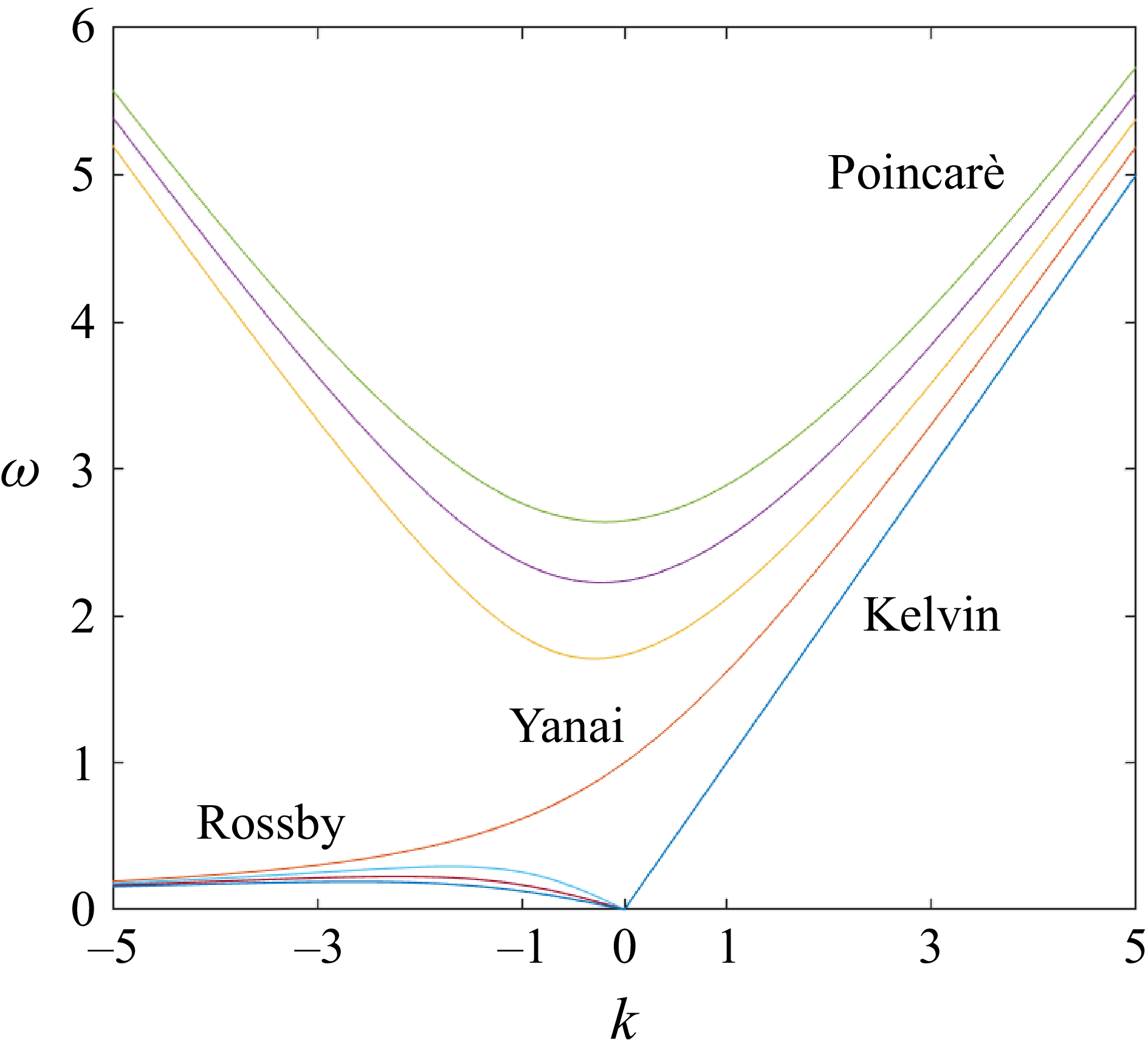
 k
 ω
 β1/2(gH)−1/4
 β1/2(gH)1/4
 β
 g
 H
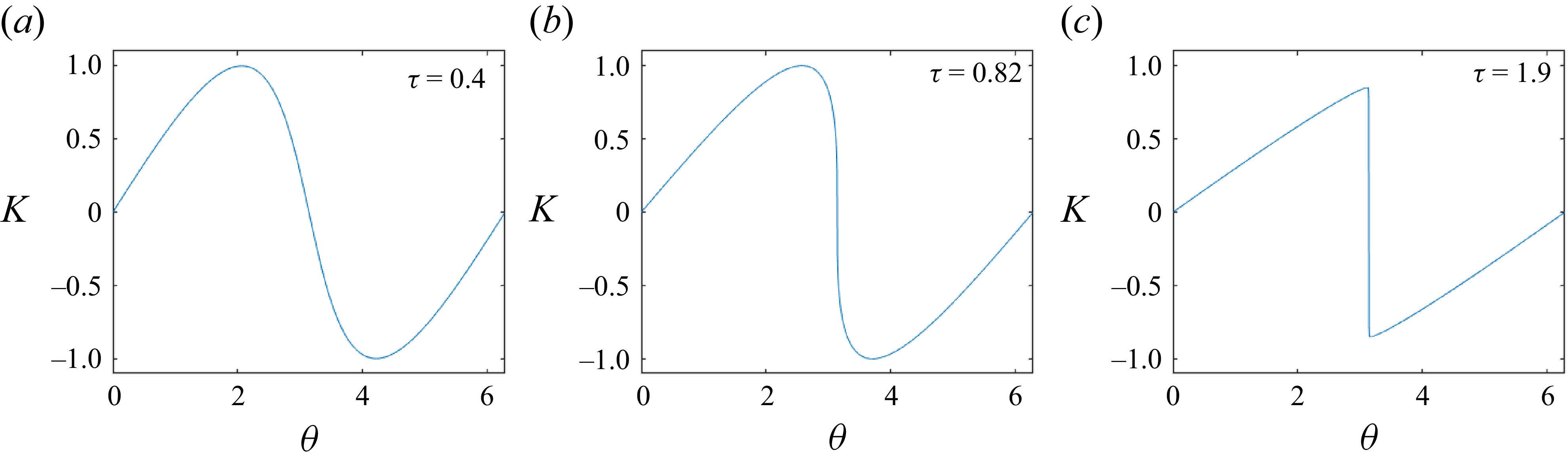
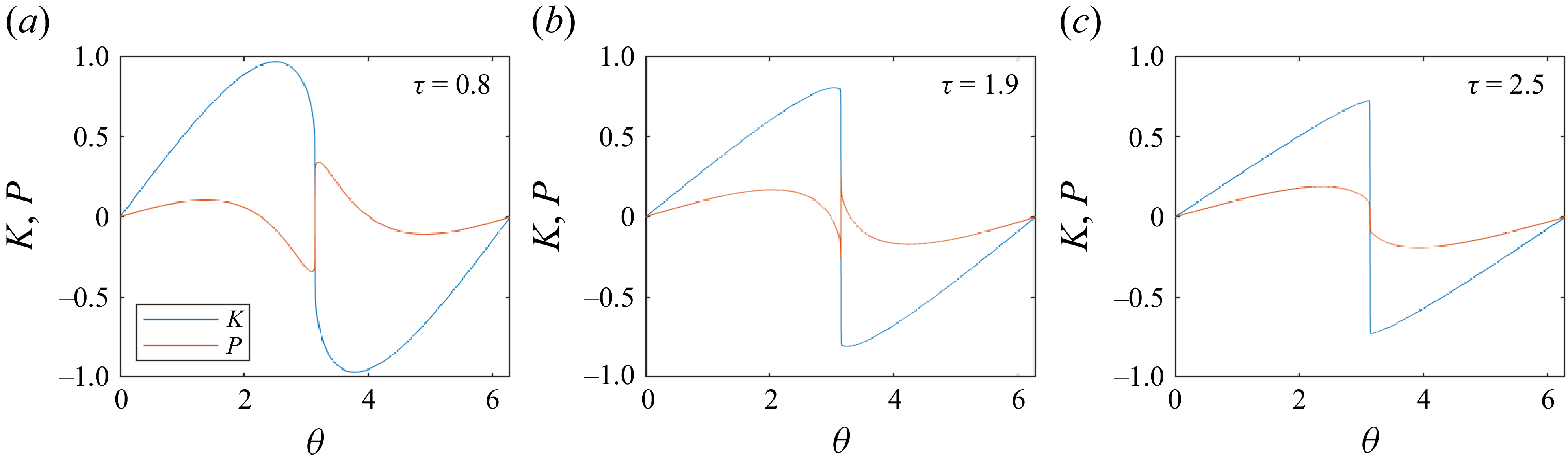
 γ=0
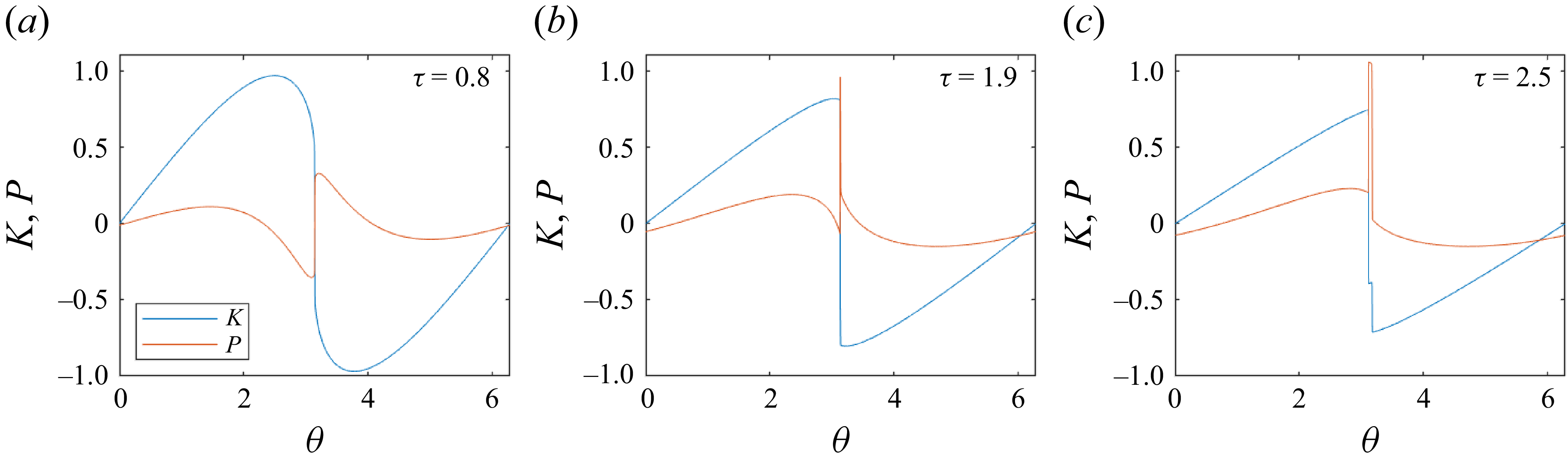
 γ=0.2
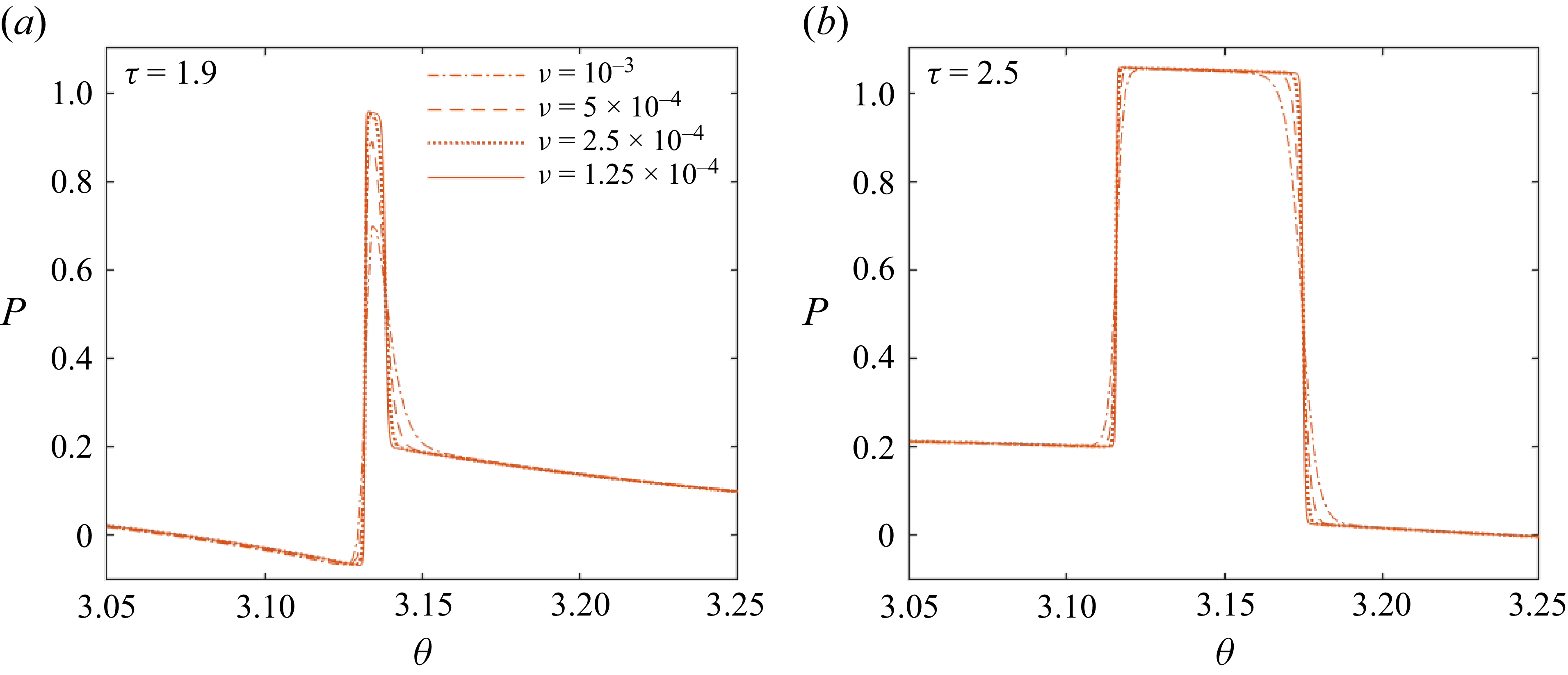
 (b)
 (c)
 ν=1.25×10⁻⁴
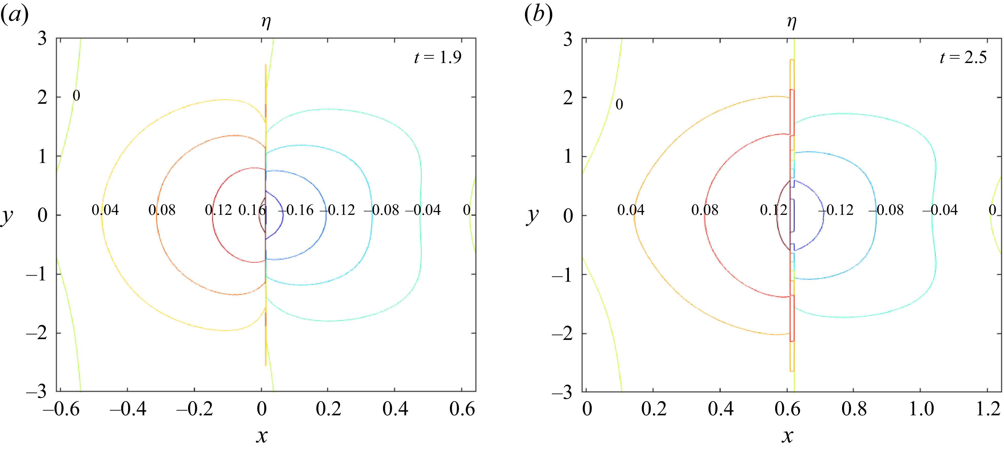
 η
 (b)
 (c)
 ε=0.2
 k=5
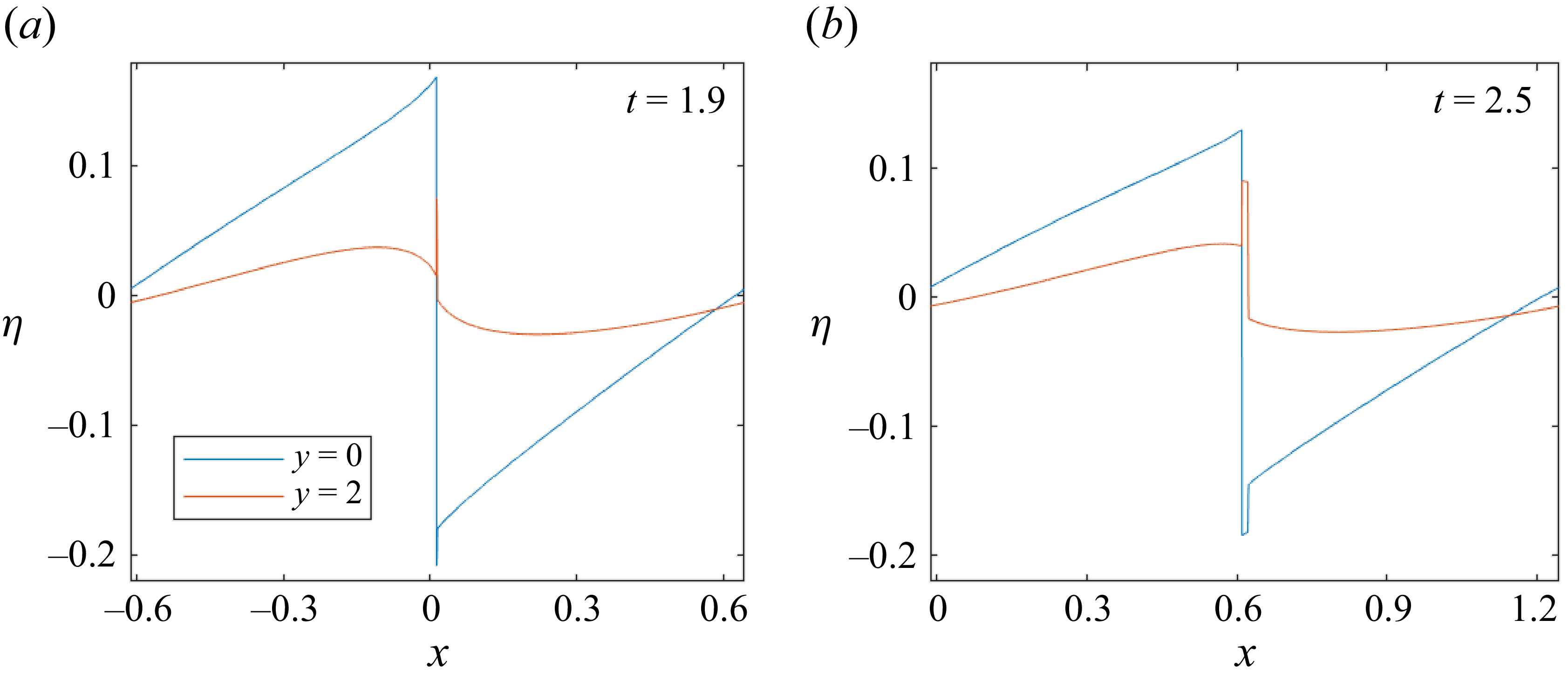
 η
 y=0
 y=2
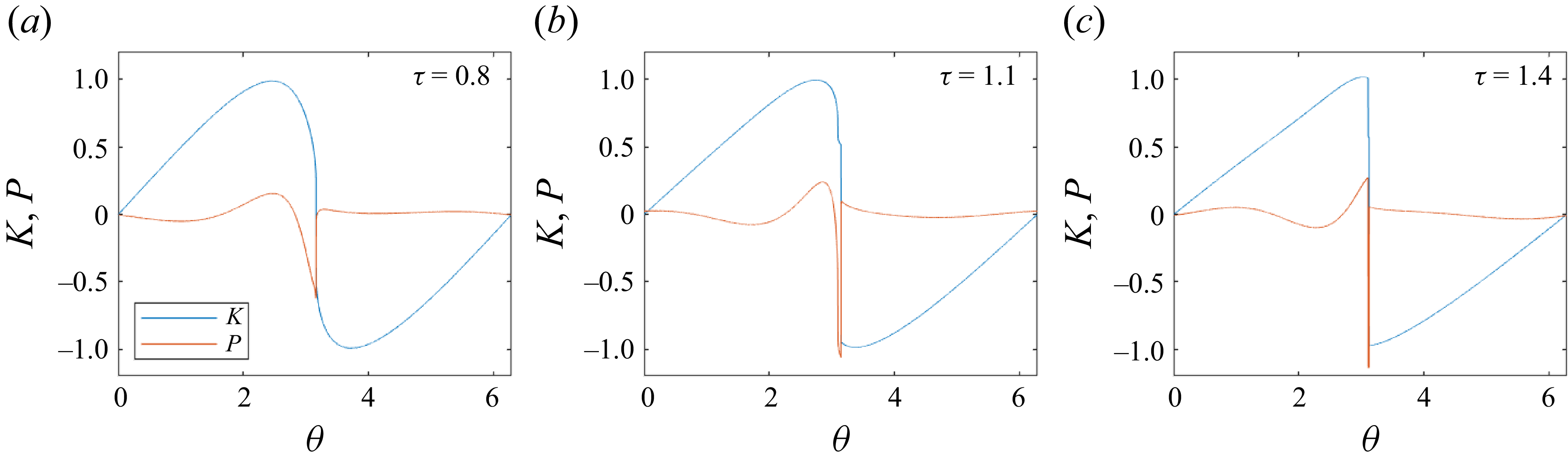
 γ=5
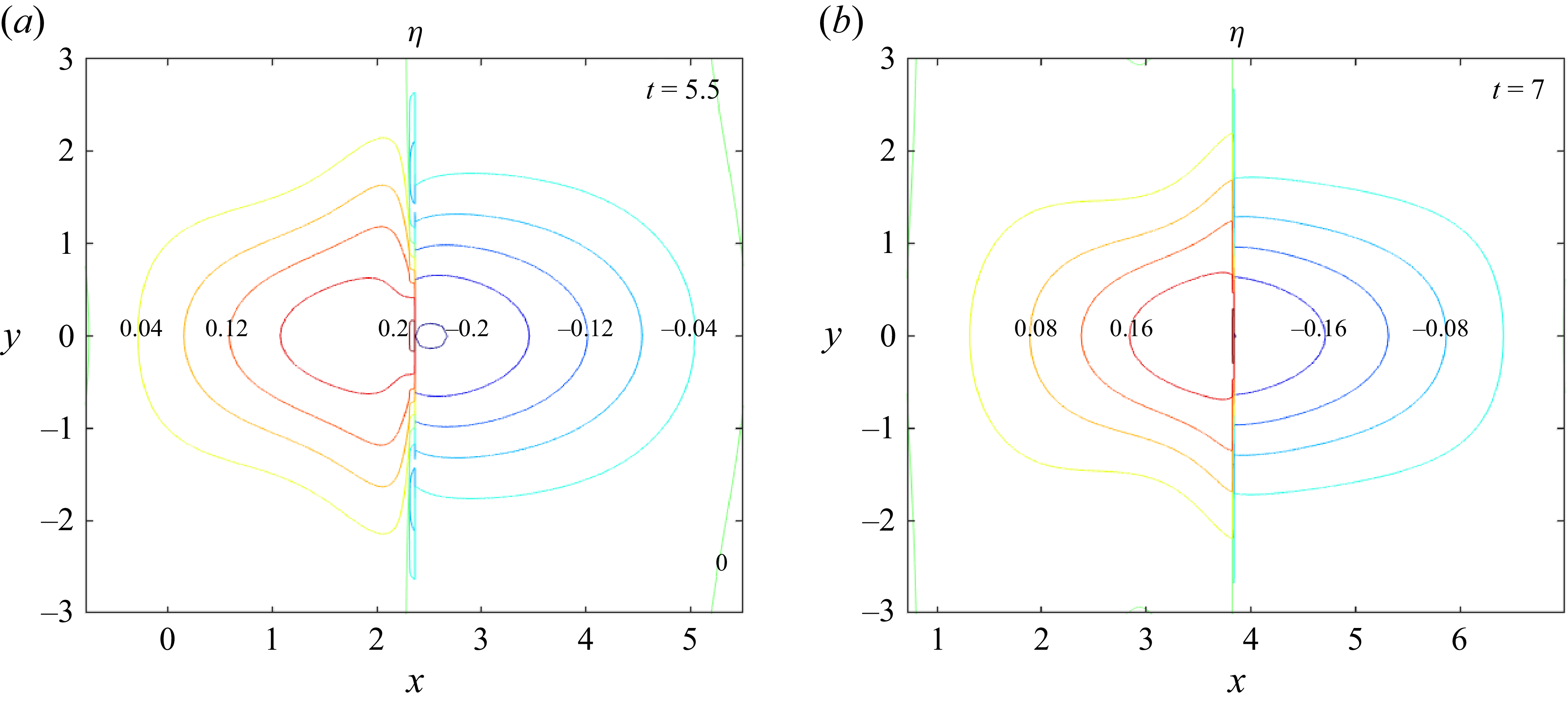
 η
 (b,c)
 ε=0.2
 k=1
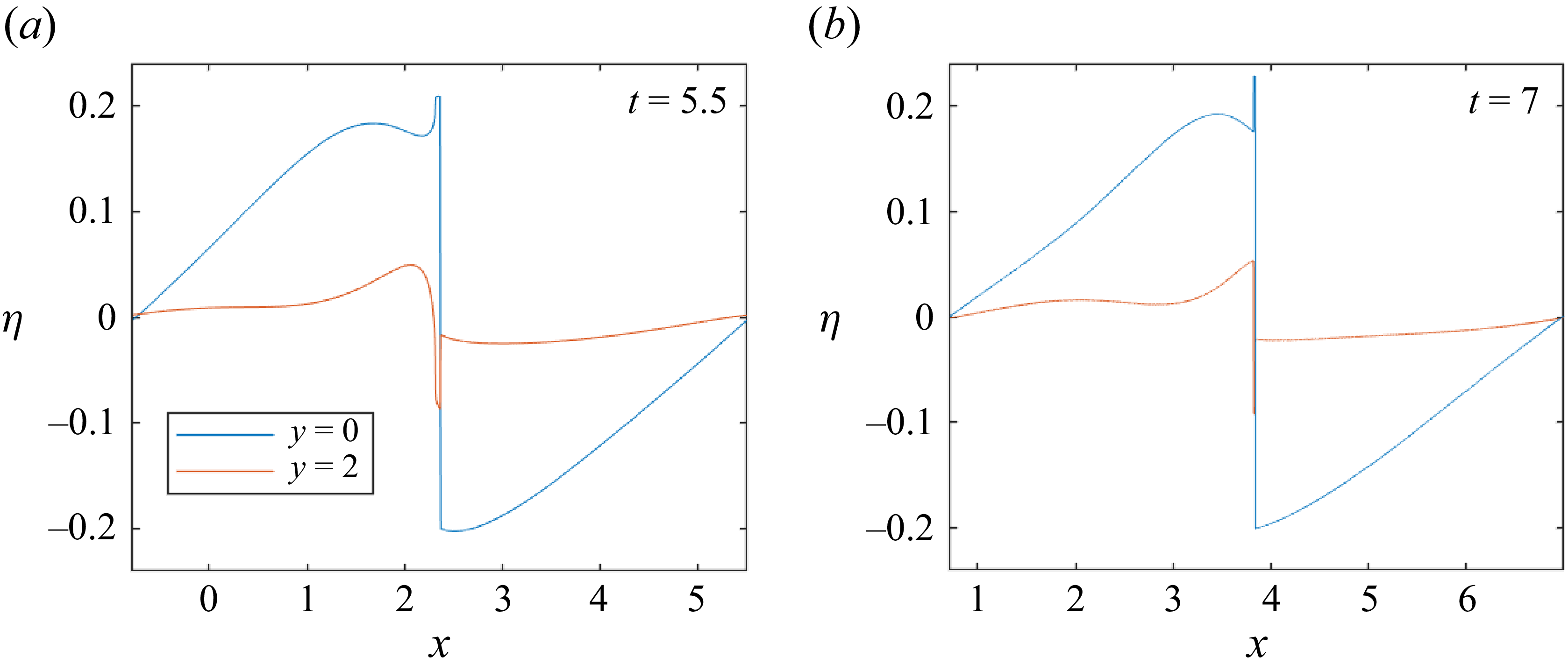
 η
 y=0
 y=2
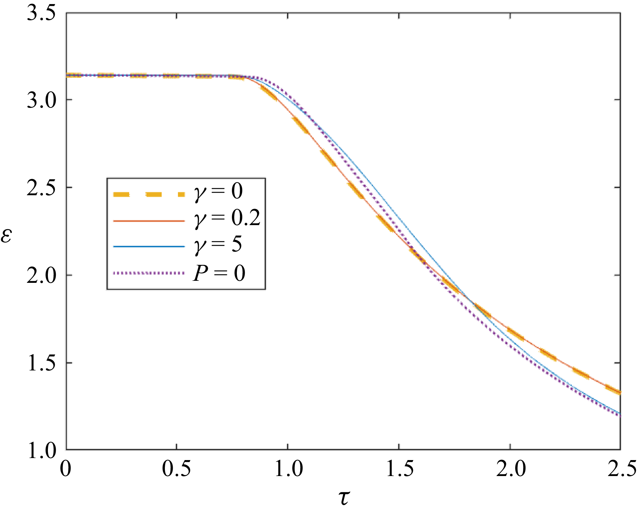
 γ
 P=0
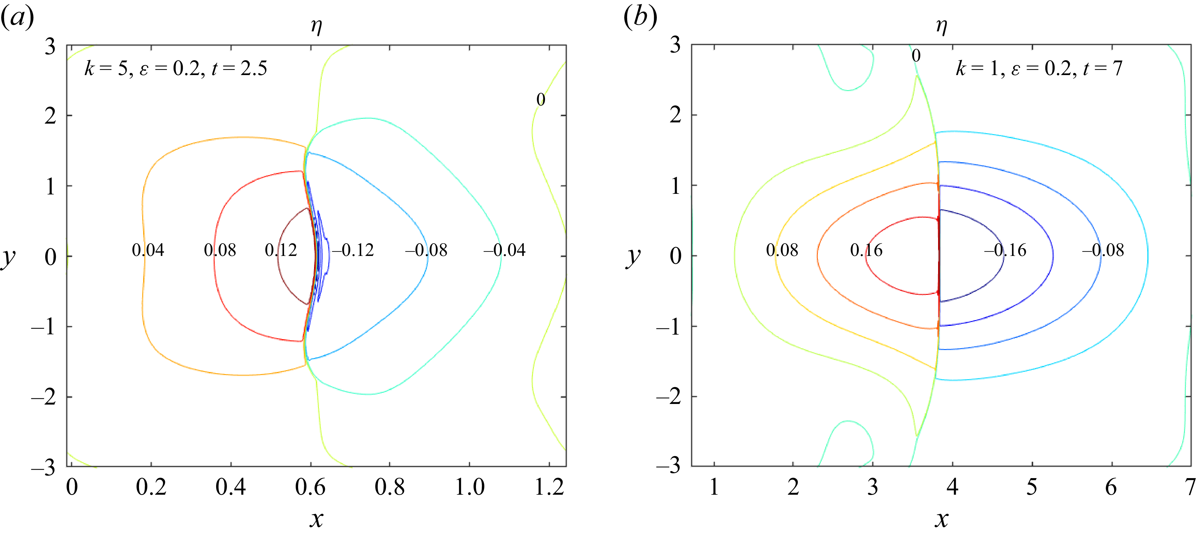
 η
 (b)
 (b)
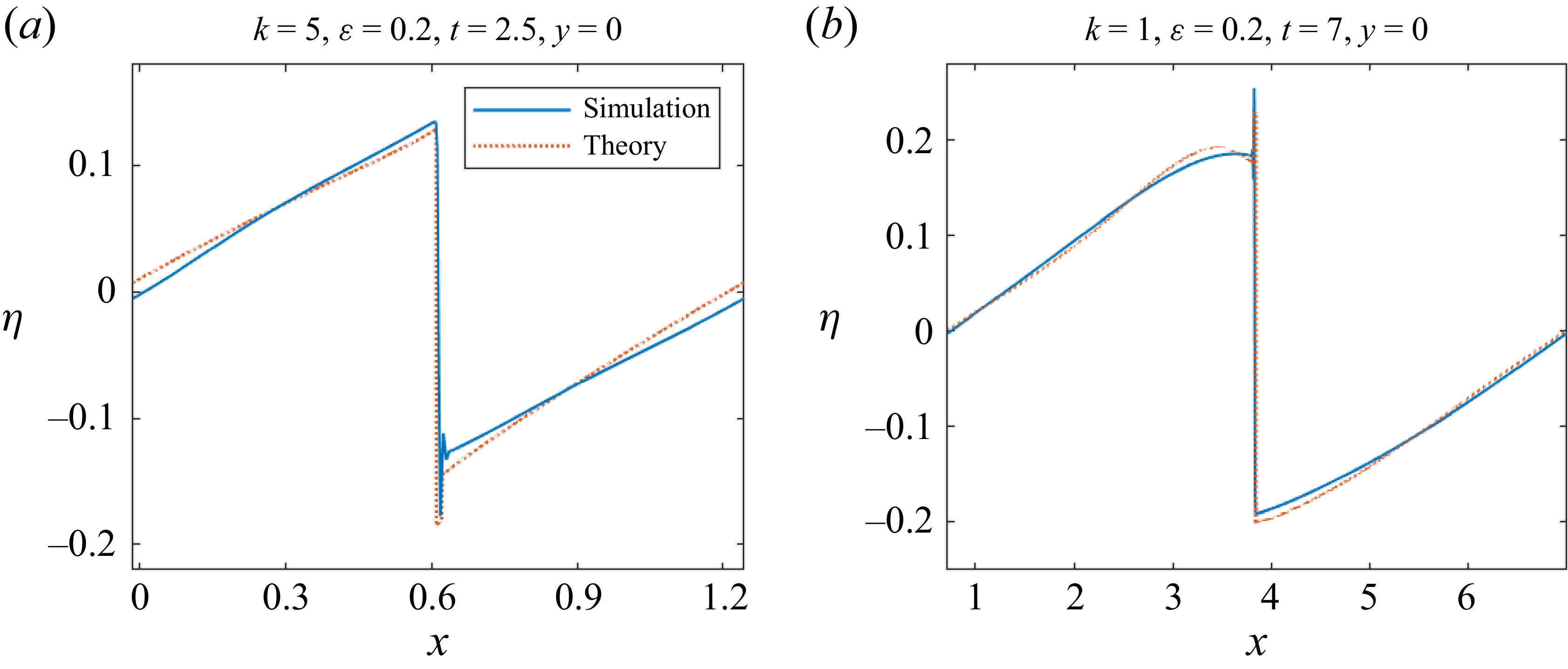
 η
 y=0


