1. Introduction
Mobile robots have been widely used in manufacturing, logistics, transportation, and other complex scenarios because of their ability to perceive the environment and navigate autonomously [Reference Qin, Shao, Wang, Yu, Jiang and Cao1]. Recent reviews have emphasized that path planning is one of the key technologies supporting autonomous mobile robot navigation [Reference Orozco-Rosas, Montiel-Ross and Movilla-Terriza2]. With the development of robotic perception, vision-based robotic systems have also been applied to structural inspection and damage recognition tasks, further increasing the demand for reliable autonomous navigation in complex environments [Reference Hu, Chen, Kang and Tang3]. Path planning connects environmental perception with motion control and aims to generate a safe and collision-free route from the start position to the target [Reference Zuo, Chen, Pan and Huang4]. For known environments, global path planning has been extensively studied through classical search-based and sampling-based methods, such as Dijkstra’s algorithm [Reference Dijkstra5], A* [Reference Hart, Nilsson and Raphael6], and RRT [Reference Qian, Liu, Tian and Bao7]. However, in environments where obstacle density varies across different regions, global planners must not only find feasible paths but also adjust their search behavior according to local environmental complexity. Studies on replanning in partially unknown environments have also shown that newly detected obstacles may require efficient path updates after the map changes [Reference Ramesh, Imeson, Fidan and Smith8].
In recent years, learning-based and sampling-based methods have shown considerable potential in robotic navigation. Reinforcement learning has been introduced into mobile robot path planning [Reference Khlif, Nahla and Safya9], and KBQ-RRT* has been proposed to improve path smoothness and kinematic feasibility in complex orchard navigation through dual-tree optimization [Reference Ye, Li, Yin, Gao and Tang10]. However, learning-based methods often require extensive training and high computational resources, while sampling-based methods may introduce randomness into the planning process. Therefore, A* and its variants remain widely used in grid-based global planning because of their deterministic search structure, clear implementation, and strong engineering applicability.
Although A* has been widely used in mobile robot global path planning, it still suffers from redundant node expansion, high memory consumption, and unsatisfactory path quality in dense or structurally complex environments. To improve search efficiency, bidirectional A* reduces redundant expansion by searching from both the start and goal directions [Reference Li, Huang, Ding, Song and Lu11]. Weighted heuristic strategies accelerate convergence by strengthening heuristic guidance, but they may sacrifice path optimality [Reference Pohl12]. Geometric constraint-based A* improves path regularity by removing unreasonable nodes during search [Reference Tang, Tang, Claramunt, Hu and Zhou13]. Another line of research has incorporated obstacle-density information into heuristic adjustment, enabling A*-based planners to reduce redundant expansion and avoid highly cluttered regions more effectively [Reference Lin, Fan, Xie, Wu and Yang14]. For example, improved LPA* has been used to reduce travel distance and navigation time [Reference Dai, Lv, Li and Zong15], while gray-wolf optimization has been integrated with A* to enhance global search capability [Reference Liu, Liu and Xiao16]. Other studies have combined A* with DWA to improve local obstacle avoidance under motion constraints [Reference Liu, Wang, Wu and Wei17]. Adaptive A* has also been fused with improved DWA to enhance overall navigation performance [Reference Liao, Hu, Luo, Li and Qu18]. These studies improve A*-based planning from the perspectives of heuristic evaluation, search acceleration, path refinement, or local planner fusion. However, the global search structure itself is still usually predefined, indicating that the adaptability of the search structure requires further investigation.
Neighborhood expansion is a key factor affecting the search behavior and path quality of A*-based planning. Zhang et al. expanded the number of search directions to accelerate node exploration [Reference Zhang, Wang and Zhou19]. Huang et al. introduced a localized neighborhood search strategy to reduce computational overhead and improve path smoothness in complex environments [Reference Huang, Zhu and Wang20]. These studies show that neighborhood configuration directly influences node expansion efficiency, path flexibility, and obstacle-avoidance performance. However, a large neighborhood may increase computational burden, whereas a small neighborhood may reduce path flexibility in cluttered or narrow regions. Therefore, a fixed neighborhood structure is difficult to maintain stable performance when the search process moves across regions with different obstacle densities. This motivates an adaptive neighborhood mechanism that can switch according to both planning progress and local obstacle density.
In addition to search efficiency, the physical executability of planned paths is also important for real mobile robot navigation, especially for omnidirectional platforms. Grid-based planning methods often generate discrete paths with angular turns, and path smoothing is usually required to improve trajectory continuity, reduce sharp turning behavior, and satisfy practical motion requirements [Reference Ravankar, Ravankar, Kobayashi, Hoshino and Peng21]. For Mecanum-wheeled robots, kinematic modeling relates target velocity commands to individual wheel angular velocities and provides a basis for feasible motion execution [Reference Palacín, Rubies, Bitriá and Clotet22]. Improved A*-based planning has also been investigated for Mecanum-wheeled robots, showing that richer search directions and path refinement can improve path quality and reduce turning points in structured environments [Reference Xu, Yu, Wang, Zhao, Chen and Liu23]. Dynamic constraints, such as maximum velocity and angular acceleration, also affect trajectory stability and positioning accuracy [Reference Park, Kim, Park and Park24]. Bhargava et al. combined A* with DWA for AGV control in static and dynamic environments [Reference Bhargava, Suhaib and Singholi25]. Gu et al. fused improved A* with DWA for inspection robots in degraded environments [Reference Gu, Liu, Li, Yuan and Bao26]. Moreover, Bhargava et al. investigated omnidirectional Mecanum-wheel AGV control using a hybrid modified A* algorithm [Reference Bhargava, Suhaib and Singholi27]. These studies improve motion feasibility, local obstacle avoidance, or control performance. However, they do not fully address how the global A* search structure should adapt to changes in local environmental complexity. Thus, it is still necessary to combine executable path generation with an environment-aware global search mechanism.
To overcome these limitations, this study proposes a Hierarchical Adaptive Neighborhood Search A* algorithm, termed HANSA*. The proposed method introduces a hierarchical adaptive mechanism that dynamically switches neighborhood structures and heuristic strategies according to planning progress and local environmental complexity. By integrating adaptive neighborhood switching, phase-dependent heuristic guidance, and two-stage path optimization, HANSA* aims to improve search efficiency, enhance adaptability to complex environments with varying obstacle densities, and generate paths with improved smoothness and executability.
2. Traditional A* algorithm
2.1. Map model
Global path planning typically uses one of three main map models: grid maps, geometric maps, and topological maps. Considering that the A* algorithm is well-suited for environments based on grids and this article focuses on its optimization and improvement, we therefore use the grid map model.
In this model, the environment is discretized into a grid of 1 m × 1 m cells, where black cells represent impassable obstacles, and white cells denote traversable free space, as shown in Figure 1.
Grid map.

2.2. A* algorithm
The A* algorithm is a widely employed heuristic search method for global path planning. The difference from Dijkstra lies in the heuristic function of the algorithm. It evaluates each potential node
 $n$
using the cost function presented in Eq. (1):
 \begin{equation} f(n)=g(n)+h(n) \end{equation}
The heuristic function
 $f(n)$
is the sum of the actual cost
 $g(n)$
from the start node to node
 $n$
, and the estimated cost
 $h(n)$
from node
 $n$
to the destination. For a node
 $n$
with coordinates
 $(x_{n},y_{n})$
and a goal node G with coordinates
 $(x_{G},y_{G})$
, there commonly used heuristic function calculation formulas are shown in Eqs. (2) to (4):
 \begin{align} h(n)&=\left| x_{n}-\mathrm{x}_{G}\right| +\left| y_{n}-\mathrm{y}_{G}\right| \\[-8pt]\nonumber\end{align}
 \begin{align} h(n)&=\sqrt{(x_{n}-x_{G})^{2}+(y_{n}-y_{G})^{2}} \\[-8pt]\nonumber\end{align}
 \begin{align} h(n)&=max(\!\left| x_{n}-x_{G}\right| ,\left| y_{n}-y_{G}\right|\! ) \end{align}
By definition,
 $g(n\_ \textit{start})=0$
. For any other node n, its cost is calculated from its parent node
 $p$
as follows.
 \begin{equation} g(n)=g(p)+\sqrt{\left(x_{p}-x_{n}\right)^{2}+\left(y_{p}-y_{n}\right)^{2}} \end{equation}
3. HANSA* algorithm improvements and design
This article proposes the HANSA* algorithm for mobile robot path planning. Its core advantage is the ability to adaptively switch between 5-neighborhood and 16-neighborhood search strategies. Based on environmental information acquired by the mobile robot, HANSA* dynamically selects the appropriate neighborhood search method and corresponding heuristic function. Furthermore, HANSA* employs a two-stage path optimization mechanism to enhance path smoothness. Applying HANSA* enables mobile robots to generate superior paths while improving path planning efficiency. A flowchart illustrating HANSA* is shown in Figure 5.
3.1. Hierarchical adaptive neighborhood search
HANSA* establishes a hierarchical adaptive search framework in which the path planning process is divided into two logical phases: an exploration phase that adopts a 16-neighborhood wide area search and an approach phase that uses a 5-neighborhood narrow area search. HANSA* achieves adaptive switching between these two phases based on two types of environmental information: the distance from the current search node to the target point and the local obstacle density around the current search node. Through the design of these two distinct search stages, HANSA* achieves significant improvements in computational efficiency and path quality.
The exploration phase of HANSA* is designed for open areas far from the target point or regions with sparse obstacles. Its objective is to maximize search efficiency by rapidly traversing large passable areas. The exploration phase employs a 16-neighborhood expansion strategy, introducing diagonal movements covering approximately a 5 × 5 area. As shown in Figure 2, the 16-neighborhood strategy provides richer movement directions and greater coverage than the traditional 8-neighborhood approach, thereby enhancing search efficiency. This phase covers longer distances in fewer steps and generates more candidate nodes.
8-neighborhood conversion to 16-neighborhood.

The approach phase prioritizes path safety and precision and is designed for narrow spaces or dense obstacle environments. When the search nears the target point or areas with high obstacle density, HANSA* switches to this phase. Upon entering the approach phase, HANSA*’s neighborhood search mode shifts from a 16-neighborhood to a 5-neighborhood. The orientation of this 5-neighborhood is not fixed but dynamically reevaluated each time the phase switches. As shown in Figure 3, the search range of the 16-neighborhood is divided into four areas, and each area is further subdivided into five neighborhood combinations with different directions.
16-neighborhood conversion to 5-neighborhood.

The search zone depends on the angle
 $\alpha$
between the vector from the current node to the target node and the x-axis, as illustrated in Figure 4. This angle
 $\alpha$
determines the zone selection in the 5-neighborhood search mode. When
 $\alpha$
falls within the range of 0° to 90°, the algorithm employs the 5-neighborhood configuration defined for zone 1. Each region is further subdivided into five distinct directional neighborhood combinations. By keeping the search focused on the target direction, the 5-neighborhood approach reduces redundant exploration in narrow passages and lowers computational overhead in dense environments.
(a) Determination of
 $\alpha$
. (b) Selecting the neighborhood.

Flowchart of HANSA*.

3.2. Dynamic switching mechanism
The dynamic switching mechanism selects the active search neighborhood based on two environmental metrics: the distance from the current node to the target and the local obstacle density. HANSA* switches to a 5-neighborhood whenever either of the following conditions is satisfied; otherwise, it continues in the 16-neighborhood.
3.2.1. Distance condition
The first type of environmental information is the distance from the current search node to the goal point. A distance switching threshold
 $D_{\textit{switch}}$
is first defined as follows:
 \begin{equation} h(n)\leq D_{\textit{switch}} \end{equation}
By comparing the distance from node
 $n$
to the goal point
 $G$
with
 $D_{\textit{switch}}$
, HANSA* determines whether the search has entered the approach region. When Eq. (6) holds, the algorithm switches from the 16-neighborhood exploration mode to the 5-neighborhood search mode. This switching strategy reduces unnecessary neighbor evaluations near the goal and provides more refined local expansion in the final approximation stage. The threshold
 $D_{\textit{switch}}$
characterizes the approach range in the grid-based search process, and its value is determined through the parameter sensitivity analysis in Section 4.1.1.
It is worth noting that
 $D_{\textit{switch}}$
serves as a search parameter during the path planning phase, rather than a triggering condition for the path execution phase. This condition is evaluated for the current search node during the node expansion process and does not directly depend on the robot’s maximum physical velocity. Velocity constraints primarily influence trajectory tracking and motion control following the generation of the global path.
3.2.2. Density condition
The second type of environmental information is the local obstacle density around the current node. HANSA* introduces the local obstacle density metric
 $\rho (n)$
to evaluate the complexity of the surrounding environment and determine whether the search should switch from the 16-neighborhood exploration mode to the more conservative 5-neighborhood search mode.
To calculate the local obstacle density around the current node, a local density evaluation window is defined on the current occupancy grid map. This window should cover the main local area that may be involved in the current neighborhood expansion, thereby reflecting the obstacle distribution around the candidate nodes. In the 16-neighborhood exploration stage of HANSA*, the minimum complete local region covered around the current node is a 5 × 5 grid area. If a 3 × 3 window is used, it can only cover the one-layer search range of the conventional 8-neighborhood and cannot sufficiently reflect the obstacle distribution around candidate nodes in the 16-neighborhood. If a larger window is used, obstacle information outside the current expansion range would be included, causing the local density estimate to be affected by more distant obstacles. This would weaken its relevance to the current neighborhood-switching decision and introduce additional computational cost. Therefore, HANSA* adopts a 5 × 5 window as the local density evaluation window. It should be noted that this 5 × 5 window is not intended to represent the full sensing range of the LiDAR. Instead, it evaluates the local obstacle distribution relevant to the current neighborhood expansion based on the obstacle information available in the current occupancy grid map. When the sensor detection range is longer, more distant obstacles can be observed and updated in the map earlier. When the sensor detection range is shorter or when obstacles appear suddenly, the corresponding obstacle information is included in the statistics of
 $N_{obs}$
within the local window only after it has been observed by the sensor and updated in the occupancy grid map.
Accordingly, the obtained
 $\rho (n)$
describes the updated local obstacle distribution in the current occupancy grid map, rather than the distribution of all potential obstacles within the full sensing range of the sensor. Let
 $N_{obs}$
denote the number of obstacle cells within the 5 × 5 local density evaluation window centered at the current node
 $n$
, and let
 $N_{\textit{total}}=25$
denote the total number of cells in this window. The local obstacle density is defined as follows:
 \begin{equation} \rho (n)=\frac{N_{obs}}{N_{\textit{total}}} \end{equation}
Where
 $\rho (n)\in [0,1]$
. A larger value of
 $\rho (n)$
indicates a denser obstacle distribution around the current node and a more complex local environment. HANSA* compares
 $\rho (n)$
with the density threshold
 $\rho _{\textit{dense}}$
. When
 $\rho (n)\gt \rho _{\textit{dense}}$
, the area around the current node is considered relatively cluttered, and the algorithm switches to the 5-neighborhood search mode to improve planning safety and accuracy. Otherwise, the algorithm continues to use the 16-neighborhood search mode to maintain efficient planning. In this article,
 $\rho _{\textit{dense}}$
is used as the local density switching threshold, and its value is determined through parameter sensitivity analysis.
3.3. Hierarchical heuristic function
Standard heuristic functions cannot be directly integrated into the adaptive neighborhood search framework, therefore, HANSA* employs a dual heuristic guidance strategy for its adaptive neighborhood characteristics. The search process is divided into an exploration phase and an approach phase, each using a specialized heuristic.
3.3.1. Exploration phase
The 16–neighborhood doubles the number of expanded neighbors compared to the 8–neighborhood, increasing computational overhead. To improve search efficiency, HANSA* uses the following dynamic hybrid heuristic. For a current node
 $n$
and the goal node
 $G$
, let their coordinates be
 $(x_{n},y_{n})$
and
 $(x_{G},y_{G})$
, respectively. Define the Euclidean distance between them as
 $P_{1}$
and the octile distance as
 $P_{2}$
:
 \begin{align} P_{1}&=\sqrt{\left(x_{n}-x_{G}\right)^{2}+\left(y_{n}-y_{G}\right)^{2}} \end{align}
 \begin{align} P_{2}&=\max\!\left(\left| x_{n}-x_{G}\right| ,\left| y_{n}-y_{G}\right| \right)+\big(\sqrt{2}-1\big)\cdot \min\left(\left| x_{n}-x_{G}\right| ,\left| y_{n}-y_{G}\right| \right) \end{align}
Let
 $d_{1}$
be the Euclidean distance from the current node n to the goal, and let
 $d_{2}$
be the Euclidean distance from the start node to the goal. The normalized search progress
 $\gamma \in \left(0\right.,\left.1\right]$
is given by:
 \begin{align} \gamma =\begin{cases} \dfrac{d_{1}}{d_{2}} & \mathrm{if}\,d_{1}\lt d_{2}\\ 1 & \text{otherwise} \end{cases} \end{align}
With these components, the dynamic hybrid heuristic function
 $h_{1}(n)$
blends
 $P_{1}$
and
 $P_{2}$
using the weight
 $\gamma$
, and the total cost
 $f(n)$
remains the sum of the actual cost
 $g(n)$
and the heuristic:
 \begin{align} h_{1}(n)&=(1-\gamma )\cdot P_{1}+\gamma \cdot P_{2} \\[-8pt]\nonumber\end{align}
 \begin{align} f(n)&=g(n)+h_{1}(n) \end{align}
When the current node
 $n$
is far from the goal,
 $d_{1}\approx d_{2}$
and thus
 $\gamma \approx 1$
; the heuristic relies mainly on the octile distance
 $P_{2}$
, which promotes fast exploration in open areas. As the search approaches the goal,
 $d_{1}$
decreases, causing
 $\gamma$
to gradually approach 0. The heuristic then converges to the Euclidean distance
 $P_{1}$
. This dynamic transformation mechanism enhances the greedy behavior of HANSA*, enabling it to converge faster in open regions. The novel dynamic hybrid heuristic is designed to complement the 16-neighborhood search, improving both path quality and computational efficiency.
3.3.2. Approach phase
When the search enters the approach phase, HANSA* switches to a 5-neighborhood and scales the heuristic with a dynamic weighting factor
 $q(n)$
to balance computational efficiency and planning accuracy. This factor maintains the goal-directed nature of the search while improving planning accuracy and search efficiency.
In this phase, HANSA* continues to use
 $\gamma$
to represent the search progress, which describes the relative distance between the current node and the target point. The variable
 $\rho (n)$
denotes the local obstacle density around the current node
 $n$
. In addition,
 $\mu$
represents the relative angle between the candidate expansion direction and the target direction. When
 $\mu =0$
, the expansion direction is aligned with the target direction; as
 $\mu$
increases, the candidate direction deviates further from the target direction. Therefore, the dynamic weighting factor and the heuristic function in the approach phase are defined as follows:
 \begin{align} q(n)&=1+\rho (n)\cdot \gamma \cdot \left(\frac{1-\cos(\mu )}{2}\right) \end{align}
 \begin{align} h_{2}(n)&=q(n)\cdot P_{1} \\[-8pt]\nonumber\end{align}
 \begin{align}f(n)&=g(n)+h_{2}(n) \end{align}
Here,
 $1-\cos \mu$
is used to describe the deviation of the candidate expansion direction from the target direction. If
 $\cos \mu$
is used directly, negative values may be introduced. Moreover,
 $\cos \mu$
reaches its maximum value when the candidate expansion direction is aligned with the target direction. Since a larger
 $q(n)$
indicates a higher heuristic cost, directly using
 $\cos \mu$
would increase the cost of expanding toward the target direction. Therefore,
 $1-\cos \mu$
is adopted to convert directional consistency into directional deviation, and the term is further divided by 2 to normalize the directional deviation to the range [0,1].
The multiplicative structure of
 $q(n)$
combines three normalized factors, corresponding to search progress, local obstacle density, and directional deviation, respectively. This design forms a hybrid heuristic adjustment mechanism. Only when the current node still requires strong goal guidance, the local obstacle density is high, and the candidate expansion direction deviates significantly from the target direction, does the product of the three factors increase noticeably, thereby strengthening the penalty for unfavorable expansion directions. Conversely, when the local environment is relatively open, the candidate expansion direction is close to the target direction, or the current node is already near the target region, a small value in any factor suppresses the increase in the weighting factor and prevents the heuristic function from being excessively amplified by a single condition. Compared with an additive structure, the multiplicative structure prevents any individual factor from directly dominating the change in the weighting factor. As a result, heuristic enhancement occurs only when multiple unfavorable conditions appear simultaneously, making it more suitable for the approach phase.
Since all three factors are normalized to the range [0,1],
 $q(n)$
is bounded within [Reference Qin, Shao, Wang, Yu, Jiang and Cao1,Reference Orozco-Rosas, Montiel-Ross and Movilla-Terriza2]. This indicates that the adjustment of the heuristic function by
 $q(n)$
is bounded. Combined with the 5-neighborhood search mode, this bounded dynamic weighting strategy enhances the local guidance capability of HANSA* in the approach phase and helps generate safer and more refined paths in obstacle-dense regions. It should be noted that
 $q(n)$
is designed as a bounded heuristic adjustment factor for improving practical search guidance, rather than as a strict optimality-preserving or formally convergence-proven weighting scheme.
3.4. Two-stage path optimization
To enhance path quality and improve computational efficiency, this article proposes a two-stage path optimization mechanism.
In the first stage, HANSA* directly integrates a local optimization mechanism into the search loop. Starting from the node currently under evaluation, the algorithm attempts to connect it to its grandparent node: if no obstacles exist between the two nodes, the intermediate node is removed, and the algorithm attempts to connect to a more distant grandparent node; conversely, if an obstacle is present between them, the intermediate node is retained, and the algorithm proceeds to the next step. Therefore, an intermediate node is removed only when the newly formed direct connection has been verified to be obstacle-free. This mechanism dynamically straightens the path during the heuristic search process, thereby effectively reducing redundant local waypoints.
In the second stage, the initial path undergoes global pruning and kinematic smoothing. Starting from the path’s origin, the algorithm iteratively selects the farthest reachable node and removes the redundant grid nodes between the current retained node and the selected node. A node is considered reachable only when the direct connection between the two nodes does not pass through any obstacle cells in the current occupancy grid map; therefore, every newly formed segment in the pruned path is checked before intermediate nodes are removed. Subsequently, cubic B-spline smoothing is applied to the pruned waypoints to generate a continuous trajectory. Since the smoothed curve may deviate from the pruned polyline, the final trajectory is discretely sampled and checked for collision. If a collision is detected, the smoothed result is rejected, and the verified pruned path is retained or regenerated with a reduced smoothing effect.
Through this two-stage optimization process, HANSA* achieves comprehensive improvements in both computational efficiency and the kinematic quality of the generated paths.
3.5. Computational complexity analysis
In this section, we analyze the space and time complexity of HANSA* and its complexity with traditional A*, Dynamically Weighted A*, and JPS. Through this analysis, we discuss how the introduction of adaptive neighborhood switching and dynamic heuristics contribute to the under-complex grid environments
3.5.1. Space complexity
Space complexity refers to the amount of memory required by an algorithm during execution. In terms of asymptotic space complexity, all four algorithms mentioned above share the same worst-case theoretical upper bound. They need to maintain open and closed sets, and their space consumption is linearly related to the total number of traversable grid cells
 $N$
in the environment, resulting in a space complexity of
 $O(N)$
. Dynamically Weighted A* changes the weights of the heuristic function but does not change the asymptotic space complexity. JPS effectively reduces the required memory through rule pruning during planning, also resulting in a space complexity of
 $O(N)$
. In the HANSA* algorithm, a hierarchical adaptive mechanism is introduced, allowing nodes to have different neighborhood state identifiers at different search stages. However, this only adds a constant-level memory overhead of
 $O(1)$
for each node’s flag bits. Consequently, the space complexity of HANSA* remains strictly
 $O(N)$
, consistent with the other three algorithms, confirming that it uses memory efficiently in the planning task without causing additional asymptotic memory burden.
3.5.2. Time complexity
All four algorithms use priority queues to implement their open sets. In A*, the node with the lowest cost is repeatedly extracted from the open set, its neighbors are evaluated, and newly generated nodes are inserted back into the queue. The time complexity of each of these steps is
 $O(\log N)$
, where N is the total number of valid grid cells in the state space. The heuristic cost calculation for neighboring nodes typically requires constant time
 $O(1)$
, therefore, the time complexity for a single node expansion is
 $O(\!\log N)$
. In the worst case, where the algorithm needs to traverse all unobstructed grid cells, after N expansions, the overall time complexity of A* is:
 \begin{equation} T_{A\ast }=O(\!\log N)\times N=O({N\log N}) \end{equation}
The Dynamically Weighted A* modifies the weights of the heuristic function. When expanding nodes, Dynamically Weighted A* needs to calculate the dynamic weight coefficients in real-time and multiply them by the heuristic cost, maintaining a time complexity of
 $O(\log N)$
. The additional weight calculation step involves only local arithmetic operations, requiring
 $O(1)$
time. Therefore, the total time complexity of Dynamically Weighted A* is:
 \begin{equation} T_{DW-A^{\ast} }=N\times \left(O(\log N)+O(1)\right)=O({N\log N}) \end{equation}
The JPS significantly reduces the number of expansions required to connect the start and end points through pruning. However, JPS may need to traverse a large number of nodes in complex maps, which does not change the worst-case asymptotic time complexity. Its worst-case time complexity remains
 $O(N\log N)$
.
During the search process, HANSA* switches between the 16-neighborhood and 5-neighborhood expansion modes according to the distance condition and the local density condition. Since different node expansions involve different numbers of neighboring candidates, the numbers of nodes expanded using the 16-neighborhood and 5-neighborhood modes are denoted as
 $N_{16}$
and
 $N_{5}$
, respectively. The total number of neighbor evaluations during the search process can then be expressed as
 $B=16N_{16}+5N_{5}$
, where
 $B$
denotes the total number of neighbor evaluations in the entire search process. For each node expansion, extracting the current minimum-cost node from the priority queue requires
 $O(\!\log N)$
time. For each evaluated neighbor, cost updating, heuristic computation, and insertion or update operations in the Open list require at most
 $O(\!\log N)$
time. Therefore, the time complexity of the search expansion stage of HANSA* can be expressed as
 $T_{\textit{search}}=O(B\log N)$
. Since the total number of expanded nodes during the search process does not exceed the total number of nodes
 $N$
in the grid map, we have
 $N_{16}+N_{5} \lt N$
. Furthermore,
 $B=16N_{16}+5N_{5}\lt 16(N_{16}+N_{5}) \lt 16N$
. Accordingly, in the worst case, the asymptotic time complexity of the search expansion stage of HANSA* remains
 $T_{\textit{search}}=O(N\log N)$
. When more nodes are expanded using the 5-neighborhood mode, the effective branching factor of HANSA* is reduced compared with a fixed 16-neighborhood expansion strategy, thereby decreasing the actual number of neighbor evaluations. In addition, HANSA* includes a two-stage path optimization process. Let
 $L$
denote the total number of grid cells traversed during all line-of-sight checks, and let
 $P$
denote the number of path points processed during B-spline smoothing. The time complexity of the path optimization stage can be expressed as
 $T_{opt}=O(L)+O(P)$
. The overall time complexity of HANSA* can be expressed as:
 \begin{equation} T_{\textit{HANSA}^{\ast} }=O(B\log N)+O(L)+O(P) \end{equation}
Here,
 $O(Blog\, N)$
represents the computational cost of the search expansion stage,
 $O(L)$
represents the cumulative cost of line-of-sight checks, and
 $O(P)$
represents the computational cost of B-spline smoothing.
3.5.3. Performance discussion and trade-offs
As will be demonstrated in Section 4.2, aggressive algorithms such as JPS or Weighted A* may require fewer expansion nodes and have slightly shorter runtimes than HANSA*. JPS prunes large portions of the search space, while Weighted A* relies on a highly greedy heuristic. However, the paths they generate are often not optimal, frequently contain hazardous sharp corners, and have inadequate obstacle clearance. In contrast, HANSA* employs adaptive mechanisms to improve overall path quality. While the 16-neighborhood evaluation and two-stage optimization add some computational overhead, they effectively reduce redundant waypoints and sharp corners. For an omnidirectional robot, avoiding a sharp corner reduces unnecessary deceleration and improves chassis stability. Ultimately, HANSA* achieves both higher path quality and shorter path length at the cost of only a marginal increase in runtime.
4. Simulation experiment
To verify the HANSA* algorithm, this article designs a series of experiments. Simulation experiments under various conditions are first conducted to evaluate the computational efficiency and stability of the proposed algorithm, with A* used as the baseline comparison. To further examine its scalability and algorithmic characteristics, HANSA* is then compared with multiple path planning algorithms on maps of different scales. Finally, real-world experiments are conducted to evaluate the practical executability of the generated paths in a physical environment.
In the following experiments, the reported Planning Time and Replanning Time denote the computation time required by the planner to generate or regenerate a path after receiving the current or updated occupancy grid map. These metrics are used to compare the algorithm-level computational efficiency of different planners, rather than the end-to-end response time of the entire robot navigation system.
To ensure consistency across all simulation and field experiments, this study defines sharp corners as turns with heading-change angles greater than or equal to 45°, denoted as Corners (≥45°). Frequent sharp corners may disrupt continuous robot motion and reduce trajectory stability.
4.1. Parameter sensitivity analysis
Before conducting the comparative experiments, the key parameters involved in the neighborhood switching mechanism of HANSA* are analyzed. The distance switching threshold
 $D_{\textit{switch}}$
is used to determine when the search process enters the approach phase, while the density threshold
 $\rho _{\textit{dense}}$
is used to determine whether the algorithm should switch to the 5-neighborhood search mode in locally cluttered regions. Since these two parameters affect both search efficiency and path quality, this section conducts parameter sensitivity analyses to determine the parameter values used in the following experiments.
4.1.1. Distance threshold analysis
The distance switching threshold
 $D_{\textit{switch}}$
determines when HANSA* enters the approach phase and switches to the 5-neighborhood search mode. Since maps with different sizes have different search distance scales,
 $D_{\textit{switch}}$
is evaluated as a percentage of the map dimension in this sensitivity analysis. To analyze the influence of this parameter on planning performance, the threshold ratio was varied from 10% to 30% on 30 × 30, 60 × 60, 100 × 100 maps, while the density threshold was fixed at
 $\rho _{\textit{dense}}=0.3$
. Each parameter setting was repeated 100 times, and the average planning time and expanded nodes were used as the main evaluation metrics.
Figure 6(a)–(c) show the sensitivity analysis results under the three map sizes. As the distance switching threshold ratio increases from 10% to 20%, both the average planning time and the number of expanded nodes decrease. When the threshold ratio further increases from 20% to 30%, these two metrics increase again. This trend is consistent across the 30 × 30, 60 × 60, 100 × 100 maps. Among the tested settings, the 20% threshold ratio achieves the lowest average planning time and the fewest expanded nodes in all three maps.
Parameter sensitivity analysis of the distance switching threshold
 $\mathrm{D}_{\text{switch}}$
under different map sizes: (a)
 $30 \times 30$
map; (b)
 $60 \times 60$
map; (c)
 $100 \times 100$
map.

Figure 6. Long description
Three line graphs depict the parameter sensitivity analysis of the distance switching threshold under different map sizes. Panel A: A line graph shows the relationship between the distance switching threshold ratio and the average planning time and expanded nodes for map size 1. The x-axis represents the distance switching threshold ratio ranging from 0.10 to 0.30. The left y-axis represents the average planning time in seconds, and the right y-axis represents the expanded nodes. The blue line with square markers indicates the average planning time, while the red dashed line with circle markers indicates the expanded nodes. The graph shows a U-shaped trend for both metrics, with the lowest values around a threshold ratio of 0.20. Panel B: A line graph shows the relationship between the distance switching threshold ratio and the average planning time and expanded nodes for map size 2. The x-axis represents the distance switching threshold ratio ranging from 0.10 to 0.30. The left y-axis represents the average planning time in seconds, and the right y-axis represents the expanded nodes. The blue line with square markers indicates the average planning time, while the red dashed line with circle markers indicates the expanded nodes. The graph shows a U-shaped trend for both metrics, with the lowest values around a threshold ratio of 0.20. Panel C: A line graph shows the relationship between the distance switching threshold ratio and the average planning time and expanded nodes for map size 3. The x-axis represents the distance switching threshold ratio ranging from 0.10 to 0.30. The left y-axis represents the average planning time in seconds, and the right y-axis represents the expanded nodes. The blue line with square markers indicates the average planning time, while the red dashed line with circle markers indicates the expanded nodes. The graph shows a U-shaped trend for both metrics, with the lowest values around a threshold ratio of 0.20.
This result can be explained by the role of
 $D_{\textit{switch}}$
in controlling the transition to the approach phase. When the threshold ratio is too small, HANSA* enters the approach phase too late, and the 16-neighborhood exploration mode is retained for a longer distance near the goal. This increases redundant neighbor evaluations and leads to more expanded nodes. In contrast, when the threshold ratio is too large, the algorithm switches to the 5-neighborhood search mode too early. Although this reduces the local branching factor, it also restricts the expansion directions prematurely and may reduce the flexibility of the search. Therefore, a threshold ratio of 20% provides a suitable balance between global exploration and local refinement. Based on this analysis,
 $D_{\textit{switch}}$
is set to 20% of the map dimension in the following experiments.
4.1.2. Density threshold sensitivity analysis
Grid resolution affects the statistics of obstacle cells within the local evaluation window, while map size changes the overall search scale and the obstacle distribution encountered by the planner. Based on these two aspects, this section conducts a parameter sensitivity analysis of the local density switching threshold
 $\rho _{\textit{dense}}$
. Maps with different sizes are first used to evaluate the performance of
 $\rho _{\textit{dense}}$
under different search scales. Then, the same 100 m × 100 m physical environment is discretized into grid maps with different resolutions to analyze the stability of
 $\rho _{\textit{dense}}$
under different map resolutions.
When
 $\rho _{\textit{dense}}$
is set to 0.3, HANSA* can switch to the 5-neighborhood search in relatively dense regions while retaining the 16-neighborhood search in open regions. As shown in Figure 7, this threshold results in a path length and planning time of 91.158 m and 14.81 ms in the 60 × 60 map and 140.391 m and 15.9 ms in the 100 × 100 map, respectively. These results indicate that
 $\rho _{\textit{dense}}=0.3$
performs well in both planning time and path length under the tested map settings. When
 $\rho _{\textit{dense}}\geq 0.4$
, the condition for switching to the 5-neighborhood becomes harder to satisfy. As a result, some relatively dense regions may still be expanded using the 16-neighborhood search, which can increase ineffective node expansion and lead to longer paths, as observed in the 30 × 30 and 100 × 100 maps. When
 $\rho _{\textit{dense}}\leq 0.2$
, HANSA* tends to switch to the 5-neighborhood too early. Although this makes the search more conservative, the reduced expansion directions may increase both the path length and the number of expanded nodes.
Parameter sensitivity analysis of the obstacle density threshold (
 ${\unicode[Arial]{x03C1}} _{\text{dense}}$
) in a complex cluttered environment: (a)
 $30 \times 30$
map; (b)
 $60 \times 60$
map; (c)
 $100 \times 100$
map.

Figure 8(a)–(c) present the results of the sensitivity analysis for
 $\rho _{\textit{dense}}$
across different grid resolutions. In this study, a single 100 m × 100 m physical environment was discretized into grid maps with resolutions of 0.5 m, 1.0 m, and 2.0 m, respectively. The results indicate that, across all three resolutions, a value of
 $\rho _{\textit{dense}}=0.3$
consistently demonstrated stable performance with respect to both planning time and path length. At a resolution of 0.5m, the number of grid cells in the map increased significantly, thereby expanding the search space and correspondingly increasing the planning time; however, the geometric form of the path could be represented with greater fidelity. Conversely, at a resolution of 2.0 m, the search space was reduced and planning time was shortened; yet, this coarser grid representation potentially resulted in an increase in the actual physical path length. Taken together,
 $\rho _{\textit{dense}}=0.3$
exhibited superior overall performance across the grid resolutions tested in this study and was subsequently selected as the density switching threshold for the experiments that followed.
Parameter sensitivity analysis of the obstacle density threshold (
 ${\unicode[Arial]{x03C1}} _{\text{dense}}$
) in a complex cluttered environment: (a)
 $0.5$
m; (b)
 $1.0$
m; (c)
 $2.0$
m.

Figure 8. Long description
Three line graphs depict the parameter sensitivity analysis of the obstacle density threshold in a complex cluttered environment. Panel A: A line graph shows the planning time and path distance for different obstacle density thresholds. The x-axis represents the obstacle density threshold, and the y-axes represent planning time in milliseconds and path distance in meters. The blue line indicates planning time, while the red line indicates path distance. Panel B: Another line graph displays similar data for a different obstacle density threshold. The axes and color scheme are the same as in Panel A. Panel C: The third line graph follows the same format, showing planning time and path distance for yet another obstacle density threshold. Each panel illustrates how planning time and path distance vary with changes in the obstacle density threshold.
4.2. Experimental comparison of different map sizes
The experiment selects three types of maps: 30 × 30, 60 × 60, and 100 × 100. The start point is uniformly set to (2,2), and the corresponding target positions are (29,29), (59,59), and (99,99) respectively. Green grids represent the start point, and blue grids represent the target position.
Figure 9 shows the paths and expanded node distributions of the HANSA* and A* algorithms. It can be seen from Figure 9 that as the map size and obstacle density increase, the path generated by A* contains more sharp corners and has poor path quality, while the path generated by HANSA* is smoother and has higher path quality. The experimental data are shown in Table I. On the 30 × 30 map, HANSA* reduced planning time by 62.9% compared to A*, expanded 15.1% fewer nodes, decreased sharp corners by 81.8%, lowered the minimum corner angle by 73.9%, and reduced path length from 41.699 m to 40.681 m. These improvements hold as map sizes increase to 60 × 60 and 100 × 100. On the 60 × 60 map, the number of sharp corners dropped to just 1 (a 91.7% reduction), and the minimum corner angle was only 3.01° (a 93.3% reduction). On the 100 × 100 map, HANSA* also outperformed A* overall, reducing planning time by 63.8% and path length by 1.76%. HANSA* employs 16-neighbor search in low obstacle density areas and 5-neighbor search in high obstacle density areas, enhancing computational efficiency and path quality. As map size and obstacle density increase, HANSA* consistently outperforms A*, validating its computational efficiency and stability. The integration of HANSA*’s search strategy with its path optimization mechanism significantly reduces both path length and planning time.
Experimental data for two algorithms on different maps

Table I Long description
A table comparing performance metrics of Traditional A* and HANSA* algorithms across different map sizes. The table has four columns: Map size, Performance metrics, Traditional A*, HANSA*, and Reduced proportion (%). It has three grouped rows for each map size: 30 x 30, 60 x 60, and 100 x 100. Each map size group contains four performance metrics: Planning time/ms, Expanded Nodes, Corners (≥45°), Min Angle (°), and path length/m. Row 1: Map size, 30 x 30. Row 2: Performance metrics, Planning time/ms. Row 3: Traditional A*, 6.2. Row 4: HANSA*, 2.3. Row 5: Reduced proportion (%), 62.9. Row 6: Performance metrics, Expanded Nodes. Row 7: Traditional A*, 113. Row 8: HANSA*, 96. Row 9: Reduced proportion (%), 15.1. Row 10: Performance metrics, Corners (≥45°). Row 11: Traditional A*, 11. Row 12: HANSA*, 2. Row 13: Reduced proportion (%), 81.8. Row 14: Performance metrics, Min Angle (°). Row 15: Traditional A*, 45. Row 16: HANSA*, 11.31. Row 17: Reduced proportion (%), 74.9. Row 18: Performance metrics, path length/m. Row 19: Traditional A*, 41.699. Row 20: HANSA*, 40.681. Row 21: Reduced proportion (%), 2.44. Row 22: Map size, 60 x 60. Row 23: Performance metrics, Planning time/ms. Row 24: Traditional A*, 32.1. Row 25: HANSA*, 9.8. Row 26: Reduced proportion (%), 69.5. Row 27: Performance metrics, Expanded Nodes. Row 28: Traditional A*, 639. Row 29: HANSA*, 528. Row 30: Reduced proportion (%), 17.4. Row 31: Performance metrics, Corners (≥45°). Row 32: Traditional A*, 12. Row 33: HANSA*, 1. Row 34: Reduced proportion (%), 91.7. Row 35: Performance metrics, Min Angle (°). Row 36: Traditional A*, 45. Row 37: HANSA*, 3.01. Row 38: Reduced proportion (%), 93.3. Row 39: Performance metrics, path length/m. Row 40: Traditional A*, 93.498. Row 41: HANSA*, 88.829. Row 42: Reduced proportion (%), 4.99. Row 43: Map size, 100 x 100. Row 44: Performance metrics, Planning time/ms. Row 45: Traditional A*, 63.8. Row 46: HANSA*, 23.1. Row 47: Reduced proportion (%), 63.8. Row 48: Performance metrics, Expanded Nodes. Row 49: Traditional A*, 1,241. Row 50: HANSA*, 1,076. Row 51: Reduced proportion (%), 13.3. Row 52: Performance metrics, Corners (≥45°). Row 53: Traditional A*, 63. Row 54: HANSA*, 36. Row 55: Reduced proportion (%), 42.9. Row 56: Performance metrics, Min Angle (°). Row 57: Traditional A*, 45. Row 58: HANSA*, 11.31. Row 59: Reduced proportion (%), 74.8. Row 60: Performance metrics, path length/m. Row 61: Traditional A*, 159.44. Row 62: HANSA*, 156.637. Row 63: Reduced proportion (%), 1.76.
Comparison of experimental results: (a)–(c) represents A*, (d)–(f) represents HANSA*.

Comparison of Experimental Results: (a)
 $30 \times 30$
map; (b)Traditional A*; (c) JPS; (d) Weighted A*; (e) Dynamically Weighted A*; (f) Liao’s method; (g) Zhang’s method; (h) Huang’s method; (i) HANSA*.

Figure 10. Long description
Panel A: A grid map showing the layout of obstacles and paths. Panel B: A grid map displaying the path generated by the Traditional A* algorithm. Panel C: A grid map showing the path generated by the JPS algorithm. Panel D: A grid map displaying the path generated by the Weighted A* algorithm. Panel E: A grid map showing the path generated by the Dynamically Weighted A* algorithm. Panel F: A grid map displaying the path generated by Liaos method. Panel G: A grid map showing the path generated by Zhangs method. Panel H: A grid map displaying the path generated by Huangs method. Panel I: A grid map showing the path generated by the HANSA* algorithm.
Compared to A*, HANSA* achieves an average reduction of 65.4% in planning time across three map types, along with an average decrease of 3% in path length. Experiments demonstrate that HANSA* outperforms A* in key metrics like search efficiency, path quality, and planning time across diverse map scenarios. This highlights HANSA*’s scalability and robustness in complex environments.
4.3. Experimental comparison of different algorithms
In the experiment of this section, HANSA* is compared with A*, JPS, Weighted A*, Dynamically Weighted A*, and the methods proposed by Liao, Zhang, and Huang to evaluate its performance. The experiment is conducted on three sizes of maps: 30 × 30, 60 × 60, and 100 × 100. For all maps, the start point is set to (2,2), and the corresponding end points are (29,29), (59,59), and (99,99), respectively.
The experimental results of the 8 algorithms on a 30 × 30 map are shown in Figure 10 and Table II, JPS, Weighted A*, and Dynamically Weighted A* expanded fewer nodes, but their path quality was inferior to that of HANSA*. Zhang’s method reduced the number of sharp corners, but it expanded more nodes and produced longer paths than HANSA*. In contrast, HANSA* achieves improvements in both efficiency and path quality through its adaptive search strategy. This strategy applies an expanded 16-neighborhood search in open areas and a precise 5-neighborhood search in complex environments. The comprehensive path optimization mechanism of HANSA* generates a trajectory with only one sharp corner, plans the shortest path, greatly improves search efficiency, and shortens planning time.
Experimental results for multiple algorithms tested on a 30 × 30 map

Table II Long description
A table comparing performance metrics of different algorithms on a 30x30 map. The table has 5 columns and 5 rows, including the header row. The columns are labeled as Metrics, Trad. A*, JPS, W-A*, DW-A*, Liao, Zhang, Huang, and HANSA*. The rows are labeled as Time (ms), Nodes, Corners (≥45°), Min Angle (°), and Path length (m). Row 1: Time (ms), Trad. A*, 7.8; JPS, 4.1; W-A*, 3.8; DW-A*, 3.3; Liao, 7; Zhang, 13; Huang, 2.8; HANSA*, 2.5. Row 2: Nodes, Trad. A*, 199; JPS, 47; W-A*, 59; DW-A*, 36; Liao, 475; Zhang, 243; Huang, 249; HANSA*, 170. Row 3: Corners (≥45°), Trad. A*, 15; JPS, 13; W-A*, 13; DW-A*, 15; Liao, 15; Zhang, 4; Huang, 6; HANSA*, 1. Row 4: Min Angle (°), Trad. A*, 45; JPS, 45; W-A*, 45; DW-A*, 45; Liao, 45; Zhang, 45; Huang, 18.43; HANSA*, 18.43. Row 5: Path length (m), Trad. A*, 42.870; JPS, 42.870; W-A*, 42.870; DW-A*, 42.870; Liao, 42.870; Zhang, 46.505; Huang, 42.246; HANSA*, 41.636.
Note: Trad. A* = Traditional A*; W-A* = Weighted A*; DW-A* = Dynamically Weighted A*. Liao, Zhang, and Huang refer to the methods proposed in Refs. [Reference Liao, Hu, Luo, Li and Qu18], [Reference Zhang, Wang and Zhou19], and [Reference Huang, Zhu and Wang20], respectively.
On the larger and more complex 60 × 60 map, the advantages of HANSA* become more pronounced, as shown in Figure 11 and Table III, outperforms all other algorithms in terms of path length, minimum turning angle, and number of sharp corners. The path generated by HANSA* features merely 4 sharp corners, boasting a minimum turn angle of 18.43° and a path length of 91.158 m. This advantage enables HANSA* to generate the shortest and smoothest path, demonstrating HANSA*’s stability and scalability.
Figure 12 illustrates that in the 100 × 100 map, both the size and obstacle density are increased. Upon examining the paths generated by eight algorithms, it is evident that HANSA* produces the smoothest one. Data from Table IV, reveals that HANSA*’s path contains no sharp corners, with a minimum turn angle of 7.59° and a path length of 140.391 m – all three metrics outperform those of the other algorithms. While the Weighted A* and Dynamically Weighted A* have shorter planning times and Zhang’s method traverse fewer nodes, their generated paths contain more sharp corners and exhibit poorer quality. Huang’s method has a planning time of 21.4 ms, whereas HANSA* achieves 15.9 ms – representing a 25.7% reduction compared to Huang’s method. HANSA* also reduces the number of expanded nodes by 43.8% compared to Huang’s method, while outperforming it in terms of sharp corners and minimum turn angle. Thus, HANSA* achieves the best overall path quality among the compared algorithms in this experiment.
As shown in Tables II–IV, compared with other algorithms, HANSA* has significant advantages in turning angle and path length, but it still requires more expanded nodes and longer planning time than JPS and Dynamically Weighted A* in some cases. This difference becomes particularly pronounced as map size and complexity increase. The primary reason is that HANSA*’s 16-neighborhood search strategy generates and evaluates more candidate nodes during planning, which enriches path directions and improves path smoothness and quality. In contrast, JPS reduces a large number of nodes through pruning, while Dynamically Weighted A* significantly reduces the number of nodes due to its greedy strategy based on the heuristically weighted function. Furthermore, HANSA*’s two-stage path optimization mechanism introduces additional computational overhead. Although the algorithm sacrifices a fraction of planning time, it delivers superior path quality and length. From a practical robotics perspective, this smooth trajectory minimizes mechanical wear, reduces operating losses, and ultimately increases the robot’s lifespan.
Experimental results for multiple algorithms tested on a 60 × 60 map

Table III Long description
A table comparing performance metrics of multiple algorithms on a 60x60 map. The table has 6 columns and 6 rows, including the header row. The columns are labeled as Metrics, Trad. A*, JPS, W-A*, DW-A*, Liao, Zhang, Huang, and HANSA*. The rows are labeled as Time (ms), Nodes, Corners (≥45°), Min Angle (°), and Path length (m). Row 1: Time (ms), Trad. A*, 54.2; JPS, 13.1; W-A*, 30.1; DW-A*, 12.1; Liao, 26.3; Zhang, 25.6; Huang, 23.6; HANSA*, 14.8. Row 2: Nodes, Trad. A*, 798; JPS, 135; W-A*, 247; DW-A*, 188; Liao, 801; Zhang, 174; Huang, 1,422; HANSA*, 743. Row 3: Corners (≥45°), Trad. A*, 16; JPS, 17; W-A*, 23; DW-A*, 29; Liao, 18; Zhang, 7; Huang, 15; HANSA*, 4. Row 4: Min Angle (°), Trad. A*, 45; JPS, 45; W-A*, 45; DW-A*, 45; Liao, 45; Zhang, 45; Huang, 18.43; HANSA*, 18.43. Row 5: Path length (m), Trad. A*, 94.083; JPS, 94.083; W-A*, 94.669; DW-A*, 96.326; Liao, 94.083; Zhang, 94.520; Huang, 92.856; HANSA*, 91.158.
Note: Trad. A* = Traditional A*; W-A* = Weighted A*; DW-A* = Dynamically Weighted A*. Liao, Zhang, and Huang refer to the methods proposed in Refs. [Reference Liao, Hu, Luo, Li and Qu18], [Reference Zhang, Wang and Zhou19], and [Reference Huang, Zhu and Wang20], respectively.
Comparison of experimental results: (a)
 $60 \times 60$
map; (b) Traditional A*; (c) JPS; (d) Weighted A*; (e) Dynamically weighted A*; (f) Liao’s method; (g) Zhang’s method; (h) Huang’s method; (i) HANSA*.

Experimental results for multiple algorithms tested on a 100 × 100 map

Table IV Long description
The table compares the performance metrics of eight algorithms on a 100 by 100 map. It has 8 columns and 6 rows. The columns are labeled as Metrics, Trad. A*, JPS, W-A*, DW-A*, Liao, Zhang, Huang, and HANSA*. The rows are labeled as Time (ms), Nodes, Corners (≥45°), Min Angle (°), and Path length (m). Row 1: Time (ms), Trad. A*, 92.7; JPS, 28.3; W-A*, 4.4; DW-A*, 4.6; Liao, 24.5; Zhang, 25.4; Huang, 21.4; HANSA*, 15.9. Row 2: Nodes, Trad. A*, 1211; JPS, 142; W-A*, 123; DW-A*, 113; Liao, 1111; Zhang, 91; Huang, 1291; HANSA*, 726. Row 3: Corners (≥45°), Trad. A*, 34; JPS, 27; W-A*, 29; DW-A*, 31; Liao, 36; Zhang, 11; Huang, 26; HANSA*, 0. Row 4: Min Angle (°), Trad. A*, 45; JPS, 45; W-A*, 45; DW-A*, 45; Liao, 45; Zhang, 45; Huang, 18.43; HANSA*, 7.59. Row 5: Path length (m), Trad. A*, 145.966; JPS, 145.966; W-A*, 145.966; DW-A*, 145.966; Liao, 145.965; Zhang, 148.442; Huang, 141.029; HANSA*, 140.391.
Note: Trad. A* = Traditional A*; W-A* = Weighted A*; DW-A* = Dynamically Weighted A*. Liao, Zhang, and Huang refer to the methods proposed in Refs. [Reference Liao, Hu, Luo, Li and Qu18], [Reference Zhang, Wang and Zhou19], and [Reference Huang, Zhu and Wang20], respectively.
Comparison of experimental results: (a)
 $100 \times 100$
map; (b)Traditional A*; (c) JPS; (d) Weighted A*; (e) Dynamically weighted A*; (f) Liao’s method; (g) Zhang’s method; (h) Huang’s method; (i) HANSA*.

Figure 12. Long description
Panel A: A scatter plot representing a map with grid points. Panel B: A scatter plot showing the path generated by Traditional A* with a red line indicating the path. Panel C: A scatter plot displaying the path generated by JPS with a red line indicating the path. Panel D: A scatter plot illustrating the path generated by Weighted A* with a red line indicating the path. Panel E: A scatter plot showing the path generated by Dynamically weighted A* with a red line indicating the path. Panel F: A scatter plot displaying the path generated by Liaos method with a red line indicating the path. Panel G: A scatter plot illustrating the path generated by Zhangs method with a red line indicating the path. Panel H: A scatter plot showing the path generated by Huangs method with a red line indicating the path. Panel I: A scatter plot displaying the path generated by HANSA* with a red line indicating the path.
4.4. Adaptive replanning under local obstacle density changes
To evaluate the adaptive replanning capability of HANSA*, this section first generates an initial path on the original occupancy grid map and then introduces unknown obstacles with different local densities along the planned route. After the obstacle information is added to the current occupancy grid map, HANSA* replans the remaining path based on the updated map and adjusts its neighborhood search strategy according to the changed local obstacle-density distribution. This experiment aims to analyze the adaptive replanning capability of HANSA* after newly detected obstacles trigger map updates.
The experimental scenario and replanning process are shown in Figure 13. In this scenario, HANSA* first generates an initial path based on the original occupancy grid map. During the simulated execution of the initial path, unknown obstacles are introduced ahead of the planned route, creating a local structural change in the updated occupancy grid map. Before the planned route enters the obstacle-affected region, HANSA* reevaluates the remaining path and performs replanning. The updated obstacle distribution changes the number of obstacle cells within the local evaluation window around the current search node, which further affects the local density value
 $\rho _{n}$
. When
 $\rho _{n}$
exceeds the switching threshold, HANSA* switches from the 16-neighborhood search mode to the more conservative 5-neighborhood search mode in dense regions. In relatively open regions, the algorithm can return to the 16-neighborhood search mode, allowing the neighborhood selection to adapt to the local obstacle distribution during replanning.
Adaptive replanning experiment under local obstacle-density changes caused by newly detected obstacles: (a) 100 × 100 experimental environment map; (b) map with newly detected unknown obstacles.

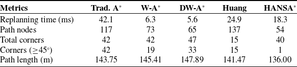
The experimental results are shown in Table V. HANSA* obtains the shortest path length of 136.00 m, uses the fewest path nodes, and produces only one sharp corner. These results indicate that HANSA* generates a higher-quality and smoother path under the tested local obstacle-density variation. Its replanning time is 18.3 ms, which is longer than W-A* and DW-A*, but shorter than Traditional A* and Huang’s method. Therefore, HANSA* does not achieve the shortest replanning time. Instead, it reduces path length, path nodes, and sharp turns, showing that the adaptive neighborhood switching mechanism improves execution-oriented path quality with a moderate increase in replanning time.
Experimental results under sudden variations in local obstacle density

Table V Long description
A table comparing metrics for different path planning algorithms. The table has five columns labeled Trad. A*, W-A*, DW-A*, Huang, and HANSA*, and six rows labeled Replanning time (ms), Path nodes, Total corners, Corners (≥45°), and Path length (m). Row 1: Replanning time (ms), Trad. A* 42.1, W-A* 6.3, DW-A* 5.6, Huang 24.9, HANSA* 18.3. Row 2: Path nodes, Trad. A* 117, W-A* 73, DW-A* 65, Huang 137, HANSA* 54. Row 3: Total corners, Trad. A* 42, W-A* 42, DW-A* 47, Huang 15, HANSA* 40. Row 4: Corners (≥45°), Trad. A* 42, W-A* 19, DW-A* 33, Huang 15, HANSA* 1. Row 5: Path length (m), Trad. A* 143.75, W-A* 145.41, DW-A* 147.89, Huang 141.47, HANSA* 136.00.
Note: Trad. A* = Traditional A*; W-A* = Weighted A*; DW-A* = Dynamically Weighted A*; Huang refers to the methods proposed in Ref. [Reference Huang, Zhu and Wang20].
4.5. Gazebo simulation and result analysis
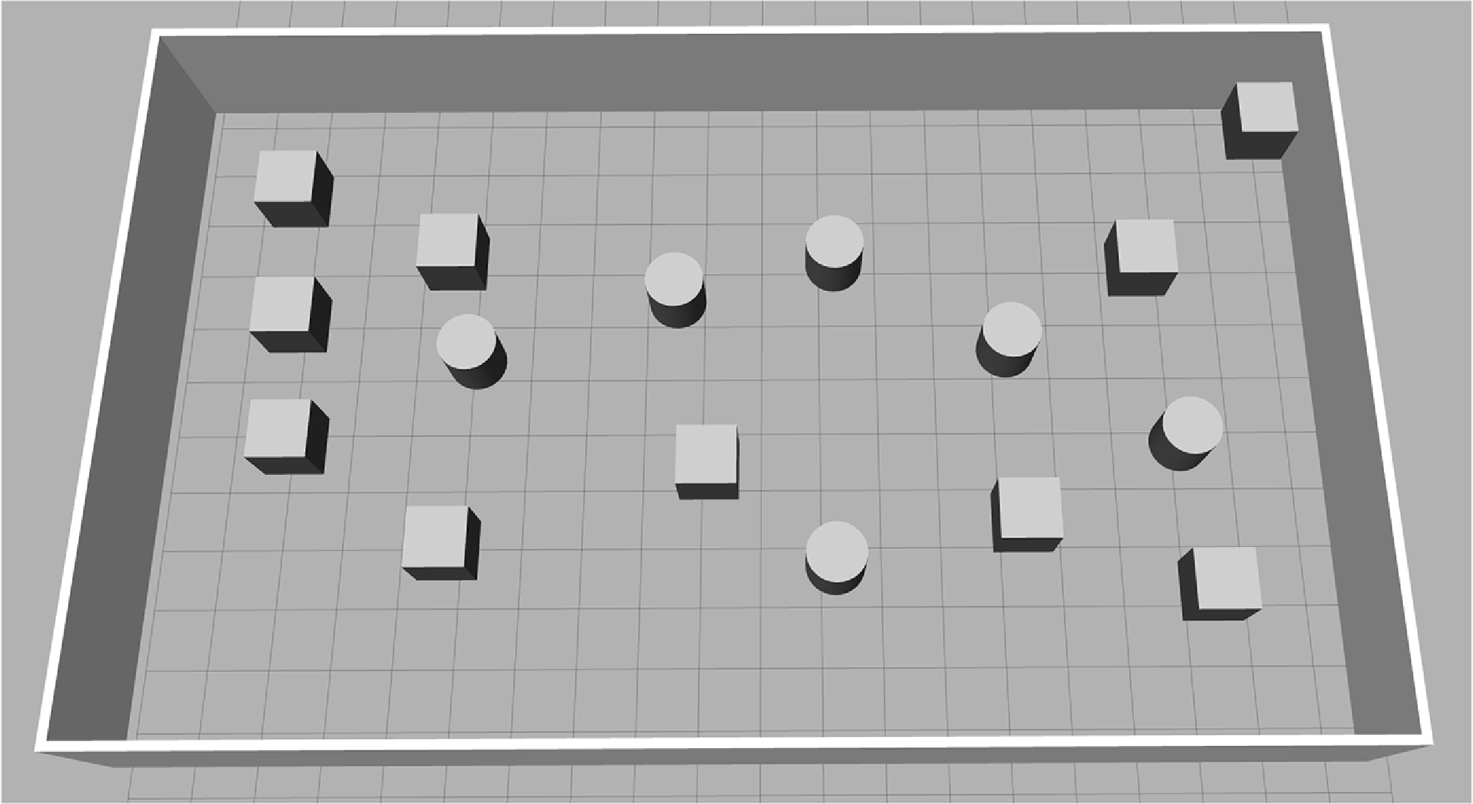
The Gazebo simulation experiments were conducted using simulation tools such as Gazebo and RViz within the ROS environment. The simulation environment is shown in Figure 14. It simulates a typical indoor environment, including open spaces and irregularly shaped obstacles.
Experimental environment.

Path planning comparison diagram: (a)Simulated environment map; (b)Traditional A*; (c) JPS; (d) Weighted A*; (e) Dynamically weighted A*; (f) Liao’s method; (g) Zhang’s method; (h) Huang’s method; (i) HANSA*.

Figure 15 shows that in the simulation environment, HANSA* generates a smoother path than other algorithms. As shown in Table VI, the path generated by HANSA* achieves the shortest and smoothest trajectory, measuring 13.48 m in length. The number of sharp corners is significantly reduced compared with most other methods, minimizing sudden stops and corners of the mobile robot. HANSA uses fewer path nodes than most comparison algorithms and achieves competitive planning computation time, thereby improving the execution-oriented quality of the generated path.
Experimental results in a simulated environment

Table VI Long description
A table comparing performance metrics of different algorithms. The table has six rows and eight columns. The columns are labeled as Metrics, Trad. A*, JPS, W-A*, DW-A*, Liao, Zhang, Huang, and HANSA*. The rows are labeled as Time (ms), Path nodes, Corners (≥45°), Min Angle (°), and Path length (m). The values in the table are as follows: Row 1: Time (ms), Trad. A*, 26.8; JPS, 18.8; W-A*, 14.3; DW-A*, 28.8; Liao, 24.1; Zhang, 13.5; Huang, 42.8; HANSA*, 17.4. Row 2: Path nodes, Trad. A*, 231; JPS, 87; W-A*, 167; DW-A*, 250; Liao, 231; Zhang, 156; Huang, 94; HANSA*, 46. Row 3: Corners (≥45°), Trad. A*, 15; JPS, 13; W-A*, 23; DW-A*, 40; Liao, 20; Zhang, 12; Huang, 10; HANSA*, 1. Row 4: Min Angle (°), Trad. A*, 45; JPS, 45; W-A*, 45; DW-A*, 45; Liao, 20; Zhang, 26; Huang, 17; HANSA*, 3. Row 5: Path length (m), Trad. A*, 14.441; JPS, 14.192; W-A*, 14.041; DW-A*, 14.097; Liao, 14.192; Zhang, 14.117; Huang, 13.978; HANSA*, 13.483.
Note: Trad. A* = Traditional A*; W-A* = Weighted A*; DW-A* = Dynamically Weighted A*. Liao, Zhang, and Huang refer to the methods proposed in Refs. [Reference Liao, Hu, Luo, Li and Qu18], [Reference Zhang, Wang and Zhou19], and [Reference Huang, Zhu and Wang20], respectively.
A key phenomenon observed in Table VI is that HANSA* uses fewer path nodes than JPS, Dynamically Weighted A*, and Zhang’s method in the Gazebo simulation. This result demonstrates the effectiveness of the proposed adaptive switching mechanism. In real-world environments, maps are typically constructed using SLAM and include an inflated layer in the cost map, resulting in highly cluttered spaces and irregular obstacle boundaries. Consequently, the local obstacle density
 $\rho (n)$
remains high for extended periods, effectively triggering the HANSA* algorithm to adaptively switch to the target 5-neighborhood search mode, thereby helping reduce redundant path points in confined spaces.
Conversely, algorithms like JPS perform poorly in such unstructured environments because their jump points are constantly interrupted by irregular obstacles, forcing them to backtrack to dense node evaluations, while Dynamically Weighted A* frequently gets trapped in local minima, requiring extensive backtracking. This demonstrates that HANSA* exhibits stronger adaptability and higher search efficiency in real-world navigation systems with complex environments.
4.6. Real experiment
The real-world experiments were conducted to evaluate the execution-oriented quality of the paths generated by HANSA* on a physical mobile robot platform. The experiments were performed on a ROS-based ABOT mobile robot equipped with Mecanum-wheels, which provide omnidirectional mobility and allow flexible changes in motion direction.
The platform uses a Jetson Nano as the ROS controller, running Ubuntu 18.04 and ROS Melodic. The chassis is driven by an OpenCRP motion controller equipped with an onboard IMU and closed-loop DC motor control. For environmental perception, the robot is equipped with a T1 LiDAR, which has a measurement range of 0.1 ∼ 8 m, a sampling rate of 4,000 samples/s, a scanning frequency of 10 Hz, and an angular resolution of 0.9°. The 2D occupancy grid map used in the real-world experiments was constructed using Gmapping based on LiDAR data. During navigation execution, odometry and IMU information from the chassis system were used to support robot localization and motion feedback. It should be noted that the real-world experiments in this study were designed to verify the execution feasibility of the paths generated by HANSA*, rather than to independently evaluate the performance of the localization system or the low-level motion controller. Therefore, accumulated odometry drift was not separately quantified as an independent evaluation metric.
Although the Mecanum-wheeled platform relaxes the strict curvature-continuity requirement compared with differential-drive robots, abrupt heading changes may still introduce unnecessary acceleration variations and unstable wheel-ground interaction during motion. Therefore, in addition to path length and planning time, the number of path nodes and sharp corners are used to evaluate the execution-oriented quality of the generated path.
4.6.1. Experiments in static environments
In the static real-world experiment, the occupancy grid map of the indoor environment was first constructed by the mobile robot using Gmapping. Based on the generated map, the same start point and target point were specified for all algorithms to compare their path planning performance. Figure 16 shows the mobile robot, the actual experimental environment, and the generated occupancy grid map.
Figure 17 presents the path planning results of different algorithms in the static real-world environment, and Table VII reports the corresponding comparison results. The evaluation metrics include Planning Time, Path Nodes, Corners, Min Angle, and Path Length.
Experimental results in real environment

Table VII Long description
A table comparing the performance of different algorithms in a static real-world environment based on various metrics. The table has 7 columns and 6 rows, including the header row. The columns are labeled as Metrics, Trad. A*, JPS, W-A*, DW-A*, Liao, Zhang, Huang, and HANSA*. The rows are labeled as Planning time (ms), Path nodes, Corners (≥45°), Min Angle (°), and Path length (m). Row 1: Planning time (ms), Trad. A*, 27.5; JPS, 28.2; W-A*, 26.3; DW-A*, 25.6; Liao, 26.7; Zhang, 25.4; Huang, 26.9; HANSA*, 25.8. Row 2: Path nodes, Trad. A*, 178; JPS, 48; W-A*, 73; DW-A*, 65; Liao, 188; Zhang, 197; Huang, 50; HANSA*, 18. Row 3: Corners (≥45°), Trad. A*, 20; JPS, 15; W-A*, 19; DW-A*, 33; Liao, 38; Zhang, 17; Huang, 5; HANSA*, 1. Row 4: Min Angle (°), Trad. A*, 45; JPS, 45; W-A*, 45; DW-A*, 45; Liao, 38; Zhang, 47; Huang, 12; HANSA*, 5. Row 5: Path length (m), Trad. A*, 9.737; JPS, 9.637; W-A*, 9.537; DW-A*, 9.544; Liao, 9.567; Zhang, 9.546; Huang, 9.242; HANSA*, 9.017.
Note: Trad. A* = Traditional A*; W-A* = Weighted A*; DW-A* = Dynamically Weighted A*. Liao, Zhang, and Huang refer to the methods proposed in Refs. [Reference Liao, Hu, Luo, Li and Qu18], [Reference Zhang, Wang and Zhou19], and [Reference Huang, Zhu and Wang20], respectively.
Mobile Robot, actual experimental environment and occupancy grid map.

Figure 16. Long description
Panel A: A mobile robot equipped with sensors and cameras, positioned on a tiled floor. Panel B: An office environment with desks, chairs, and various obstacles scattered around. Panel C: An occupancy grid map representing the layout of the office environment, showing walls and obstacles as black areas and free space as white areas.
Pathfinding results for various algorithms: (a) Traditional A*; (b) JPS; (c) Weighted A*; (d) Dynamically weighted A*; (e) Liao’s method; (f) Zhang’s method; (g) Huang’s method; (h) HANSA*.

Figure 17. Long description
Panel A: Traditional A* algorithm showing a path with multiple turns and some redundant node expansions. Panel B: JPS algorithm displaying a more streamlined path with fewer turns. Panel C: Weighted A* algorithm presenting a path with fewer turns and reduced redundancy. Panel D: Dynamically weighted A* algorithm showing a path with adaptive turns and reduced node expansions. Panel E: Liaos method illustrating a path with improved regularity and fewer unreasonable nodes. Panel F: Zhangs method depicting a path that avoids highly cluttered regions and reduces redundant expansions. Panel G: Huangs method showing a path with enhanced global search capability and reduced travel distance. Panel H: HANSA* algorithm displaying a path with improved overall navigation performance and adaptive search structure.
As shown in Table VII, HANSA* achieves the shortest path length of 9.017m and uses only 18 path nodes, fewer than all comparison algorithms. In terms of path smoothness, HANSA* produces only one sharp corner, while the other algorithms generate more sharp turns. These results indicate that HANSA* generates a higher-quality and smoother path. The reduction in path nodes and sharp corners further supports the effectiveness of the adaptive neighborhood switching mechanism. In the static indoor environment, HANSA* reduces redundant path points and sharp heading changes, making the generated path more suitable for execution on the mobile robot platform.
Overall, the results show that HANSA* generates a shorter and smoother path in the tested static real-world environment, with fewer path nodes and fewer sharp turns, indicating better execution-oriented path quality for the mobile robot platform.
4.6.2. Real-world replanning with unknown obstacles
We utilized SLAM to construct a static map encompassing both complex indoor environments and long, narrow corridors. During the navigation task, unknown obstacles were introduced in selected regions along the planned route to create local map changes in the real-world environment. After the obstacle information was detected and updated in the occupancy grid map, HANSA* replanned the remaining path based on the updated map. This experiment evaluates how HANSA* adapts its replanning strategy when newly detected obstacles cause local changes in the occupancy grid map. The experimental results are presented in Table VIII and Figure 18. Figure 18(a) shows the narrow corridor environment, while the complex indoor environment is similar to the static real-world environment shown in Figure 16. Figure 18(b) and (c) show the regions with unknown obstacles, and Figure 18(d) presents the replanned path after the unknown obstacles are introduced.
Experimental results in an unknown environment

Table VIII Long description
A table comparing metrics for different navigation strategies. The table has five rows and six columns. The columns are labeled Trad. A*, JPS, W-A*, DW-A*, Huang, and HANSA*. The rows are labeled Replanning time (ms), Path nodes, Corners (≥45°), and Path length (m). The values in the table are as follows: Row 1: Trad. A*, 88.3; JPS, 114.2; W-A*, 35.7; DW-A*, 20.2; Huang, 57.9; HANSA*, 51.8. Row 2: Trad. A*, 455; JPS, 72; W-A*, 246; DW-A*, 182; Huang, 466; HANSA*, 315. Row 3: Trad. A*, 36; JPS, 33; W-A*, 153; DW-A*, 167; Huang, 25; HANSA*, 0. Row 4: Trad. A*, 57.982; JPS, 68.911; W-A*, 50.015; DW-A*, 51.904; Huang, 46.628; HANSA*, 42.243.
Note: Trad. A* = Traditional A*; W-A* = Weighted A*; DW-A* = Dynamically Weighted A*; Huang refers to the methods proposed in Ref. [Reference Huang, Zhu and Wang20].
Replanning experiment with unknown obstacles: (a) narrow corridor environment; (b), (c) regions with unknown obstacles; (d) replanned path after unknown obstacles are introduced.

After the unknown obstacle information is updated in the occupancy grid map, the map state changes accordingly, and the algorithm replans the remaining path based on the updated map. As shown in Table VIII, HANSA* achieves the shortest path length of 42.243 m and produces no sharp corners under the Corners metric. Compared with JPS, Weighted A*, and Dynamically Weighted A*, the path generated by HANSA* avoids noticeable oscillations and large detours. Although Huang’s method also produces a relatively short path, its replanning time and number of path nodes are higher than those of HANSA*. These results indicate that HANSA* generates a higher-quality and smoother path in the tested unknown-obstacle scenario.
The improved path quality is mainly related to the two-stage path optimization mechanism and the local-density-based neighborhood switching strategy. In environments where open corridors and complex spaces alternate, HANSA* may require longer replanning time than faster heuristic methods such as Weighted A* and Dynamically Weighted A*. However, this additional computation helps reduce path length and sharp turns, improving the execution-oriented quality of the generated path for the mobile robot platform.
5. Conclusion
This article proposes a hierarchical adaptive neighborhood search A* algorithm, termed HANSA*, which dynamically adjusts its neighborhood search strategy according to path-planning progress and local environmental complexity. HANSA* introduces phase-specific heuristic functions for the 16-neighborhood and 5-neighborhood search structures and integrates a two-stage path optimization mechanism to jointly improve path quality and planning efficiency. Simulation and real-world experimental results demonstrate that HANSA* outperforms the comparison algorithms considered in this study. Particularly in dense and complex environments, HANSA* effectively mitigates common limitations of traditional A* methods, such as path redundancy and excessive sharp turns, while showing improved adaptability and robustness under local obstacle-density variations and updated occupancy-grid maps.
As a global path planner, HANSA* is mainly designed to improve search efficiency, path smoothness, and adaptive replanning performance when local structural changes are reflected in the occupancy grid map. The current study does not explicitly model continuously moving obstacles, sensor detection delays, localization update delays, or the full end-to-end latency of the perception-localization-planning-control pipeline. For scenarios involving continuously moving obstacles, such as pedestrians or autonomous vehicles, future work will integrate HANSA* with local path planning and real-time obstacle avoidance algorithms to enhance dynamic-environment navigation capability. In addition, because the current obstacle-density assessment relies on a fixed-size local evaluation window associated with the grid resolution, future research will develop a scale-adaptive perception model to improve generalization across different sensor accuracies, map resolutions, and robot platforms.
Author contributions
D. C. and J. J. conceived and designed the study; D. C. performed the methodology, software, and validation; D. C. analyzed the data and wrote the original draft; J. J., J. W., Y. S., J. Z. and Y. R. reviewed and edited the manuscript; J. J. provided supervision, project administration and funding acquisition. All authors have read and agreed to the published version of the manuscript.
Financial support
This research was funded by the National Natural Science Foundation of China (Grant Nos. 62473344 and 72071183), the Key Project of Science and Technology of Shanxi Province (Grant No. 98008304), the Opening Foundation of Shanxi Key Laboratory of High Performance Battery Materials and Devices (Grant No. 2022HPBMD01002), and the Graduate Education Innovation Project of Shanxi Province (Grant No. 2023SJ234).
Competing interest
The authors declare no competing interest.
Ethical approval
The authors have nothing to report.
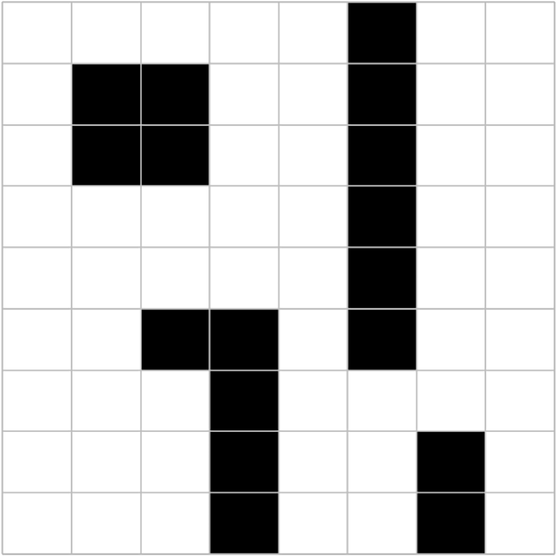
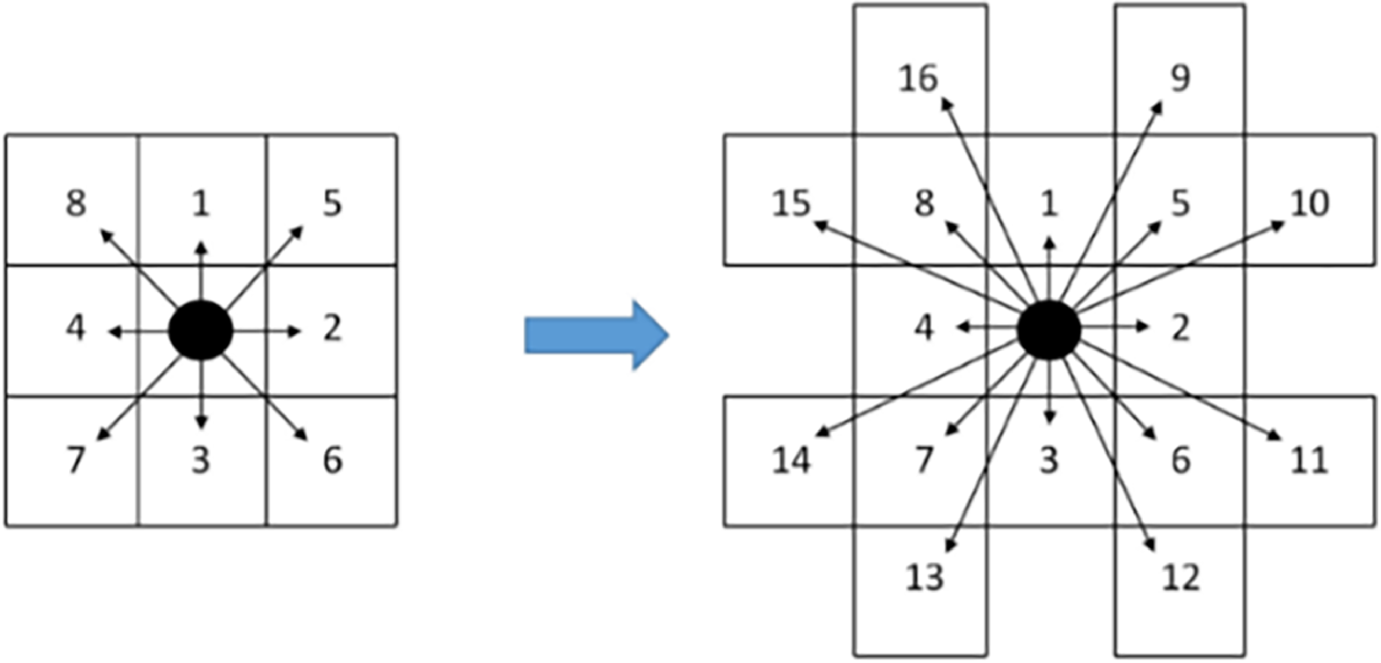


 α
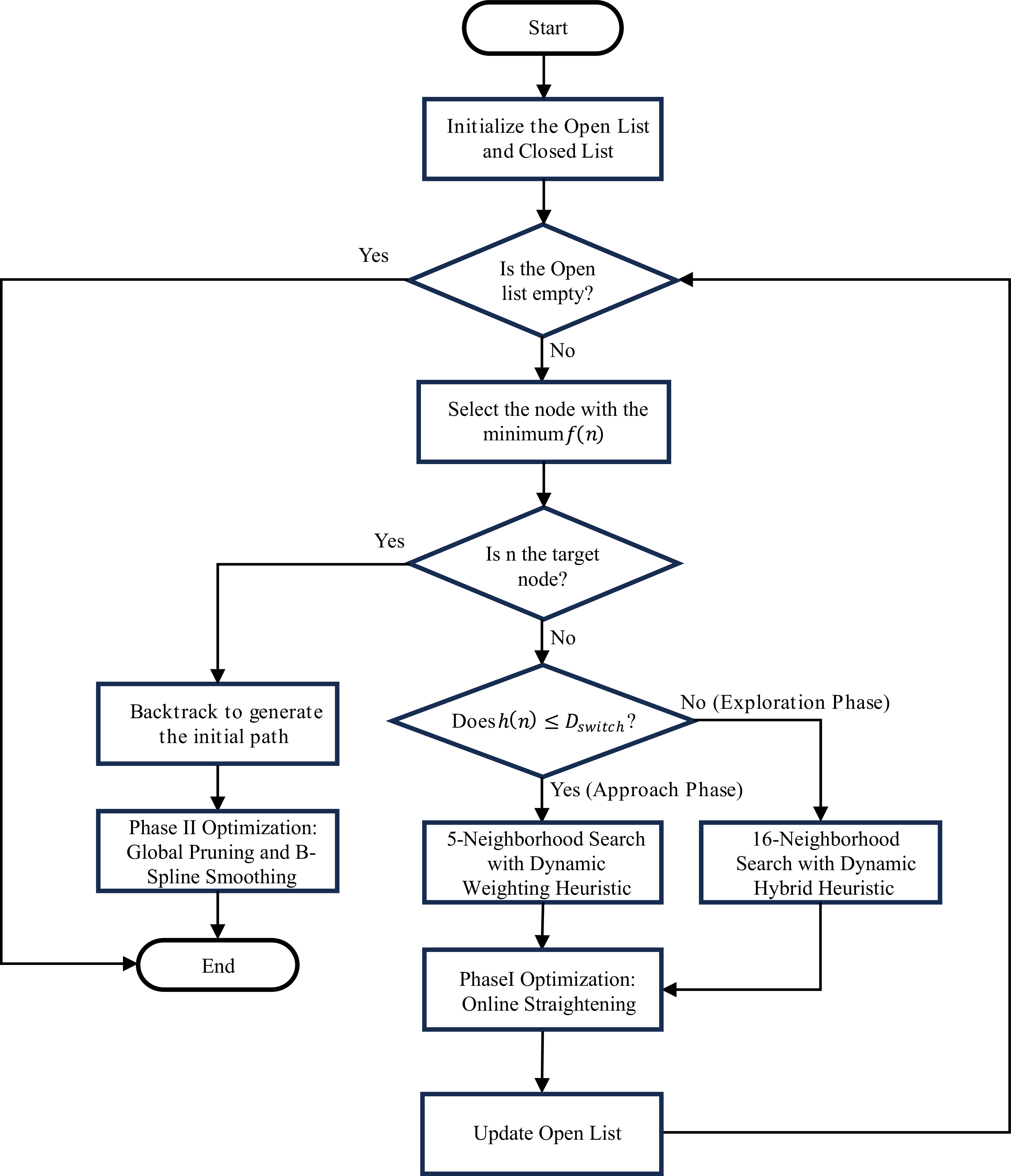

 Dswitch
 30×30
 60×60
 100×100

 ρdense
 30×30
 60×60
 100×100

 ρdense
 0.5
 1.0
 2.0
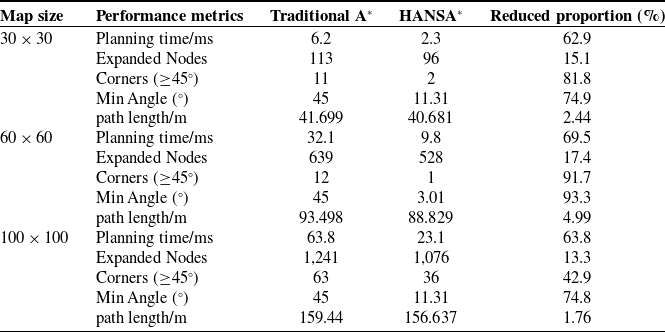


 30×30



 60×60


 100×100