



1. Introduction
Shock–droplet interactions manifest in various scenarios, such as the damage incurred by aircraft or space vehicles from raindrops (Ando Reference Ando2010), the secondary breakup of liquid jets in scramjets (Liu et al. Reference Liu, Wang, Sun, Wang and Wang2018), and applications in ultrasonic therapy (Coralic Reference Coralic2015; Shpak et al. Reference Shpak, Verweij, de Jong and Versluis2016). Investigating these interactions presents challenges due to their minute spatial and temporal scales.
Prior studies on shock–droplet interactions have extensively documented droplet morphology. Investigations have delved into the parameters governing droplet fracture morphology, including the Reynolds number, Weber number, Ohnesorge number, density ratio and viscosity ratio (Lane Reference Lane1951; Engel Reference Engel1958; Hanson, Domich & Adams Reference Hanson, Domich and Adams1963; Nicholls & Ranger Reference Nicholls and Ranger1969; Hsiang & Faeth Reference Hsiang and Faeth1992, Reference Hsiang and Faeth1995; Liu & Reitz Reference Liu and Reitz1997; Joseph, Belanger & Beavers Reference Joseph, Belanger and Beavers1999; Lee & Reitz Reference Lee and Reitz2000; Aalburg, Van Leer & Faeth Reference Aalburg, Van Leer and Faeth2003; Kékesi, Amberg & Wittberg Reference Kékesi, Amberg and Wittberg2014; Meng Reference Meng2016). The dynamic attributes of droplets have been assessed through parameters such as longitudinal and transverse diameters, drag coefficient and surface area. Breakup modes have been categorized into bag mode, bag and stamen mode, multi-bag mode, sheet thinning mode and catastrophic mode (Pilch & Erdman Reference Pilch and Erdman1987). Corresponding feature numbers for each mode have also been documented (Guildenbecher, López-Rivera & Sojka Reference Guildenbecher, López-Rivera and Sojka2009; Zhao et al. Reference Zhao, Liu, Li and Xu2010). Theofanous & Li (Reference Theofanous and Li2008) utilized laser-induced fluorescence in experiments to offer detailed insights, demonstrating that the catastrophic breakup mode is an experimental artefact. Breakup modes have been reclassified into two categories: the Rayleigh–Taylor piercing mode for  $We < 100$ based on Rayleigh–Taylor instability, and the shear-induced entrainment mode for
 $We > 1000$ based on Kelvin–Helmholtz instability (Theofanous & Li Reference Theofanous and Li2008; Theofanous Reference Theofanous2011; Theofanous et al. Reference Theofanous, Mitkin, Ng, Chang, Deng and Sushchikh2012).
Through advances in experimental measurement, the phenomenon of cavitation or the presence of cavities in droplets has been observed in pertinent experiments involving early-stage shock–droplet interactions (Sembian et al. Reference Sembian, Liverts, Tillmark and Apazidis2016) and droplet–wall impingement (Field, Dear & Ogren Reference Field, Dear and Ogren1989; Obreschkow et al. Reference Obreschkow, Kobel, Dorsaz, De Bosset, Nicollier and Farhat2006, Reference Obreschkow, Dorsaz, Kobel, de Bosset, Tinguely, Field and Farhat2011; Field et al. Reference Field, Camus, Tinguely, Obreschkow and Farhat2012). Any liquid can enter a metastable state by being overheated above its boiling point temperature or stretched below the saturated vapour pressure. Equilibrium is eventually restored through nucleation (cavitation) of steam bubbles (Caupin & Herbert Reference Caupin and Herbert2006). The present study delves into the cavitation phenomenon induced by stretching (negative pressure) rather than boiling. When a cavity ruptures, it generates a series of shock waves (Wu, Xiang & Wang Reference Wu, Xiang and Wang2018), potentially influencing subsequent droplet deformation and breakup (Bhattacharya Reference Bhattacharya2016), thereby possibly hastening equipment damage (Philipp & Lauterborn Reference Philipp and Lauterborn1998; Kodama & Tomita Reference Kodama and Tomita2000; Brujan et al. Reference Brujan, Keen, Vogel and Blake2002). According to classical nucleation theory (Debenedetti Reference Debenedetti1996), pure liquid water should withstand pressures exceeding  $-$100 MPa (Caupin Reference Caupin2005; Azouzi et al. Reference Azouzi, Ramboz, Lenain and Caupin2013).
The initial phase of shock–droplet interaction (prior to the shock wave completely traversing the droplet) receives limited attention due to the minimal deformation of droplet shape and the involvement of small time scales. Sembian et al. (Reference Sembian, Liverts, Tillmark and Apazidis2016) were the first to observe cavities within droplets during the early stages of shock–droplet interaction in experimental settings. Their findings revealed that transmitted waves within the droplet reflect and concentrate as expansion waves upon reaching the downstream wall (i.e. gas–liquid interface) of the droplet, creating a negative peak pressure (NPP) point that triggers cavitation. Biasiori-Poulanges & Schmidmayer (Reference Biasiori-Poulanges and Schmidmayer2023) conducted a phenomenological analysis of shock-induced cavitation in droplets using a multi-phase modelling approach. The critical pressure relaxation rate crucial to the numerical model was ascertained by comparing numerical outcomes with the Keller–Miksis model and related experiments. Additionally, adjustments were made in predicting the bubble cloud to factor in the magnitude of the expansion wave. Schmidmayer & Biasiori-Poulanges (Reference Schmidmayer and Biasiori-Poulanges2023) examined the geometrical effects on shock-induced cavitation in droplets, considering various aspects such as the shape of the transmitted wavefront and the droplet's geometry (cylindrical versus spherical). Determining the critical Mach numbers for cavitation onset in the column and droplet, two cavitation regimes were identified based on transmitted wavefront geometry. Xu et al. (Reference Xu, Fan, Wu, Wen and Wang2023) explored the impact of planar shock waves with varying intensities on liquid droplets using a numerical method capable of resolving compressible multi-phase flow issues without phase change.
Xiang & Wang (Reference Xiang and Wang2017) simulated the interaction between a shock wave and a cylindrical droplet containing an air cavity, investigating the impacts of varying shock wave intensities and cavity sizes. Liang et al. (Reference Liang, Jiang, Wen and Liu2020) conducted a quantitative analysis of how the relative size and eccentricity of the cavity affect the motion and deformation of hollow droplets in experiments. Liu (Reference Liu2021) observed the deformation processes wherein the vapour cavity first compresses and then expands during shock tube experiments, deriving an equation predicting the vapour bubble collapse process. Previous studies examined the effects of cavities within droplets, assuming a constant-diameter cavity initialization. However, in reality, the cavity expands as pressure decreases. Evaluating the fundamental reasons influencing shock–droplet interactions is challenging, making it difficult to assess cavity formation, size, location and temporal evolution accurately.
This study focuses primarily on identifying the location of the NPP during the early stages of shock–droplet interaction, a key driver of cavitation. Research by Sembian et al. (Reference Sembian, Liverts, Tillmark and Apazidis2016) indicated a constant cavity location approximately 19 $\%$ of the droplet's diameter from the downstream wall. Wu et al. (Reference Wu, Xiang and Wang2018) performed a theoretical examination of internal wave structures within droplets in droplet–wall impingement studies, suggesting a consistent cavity position approximately one-third of the diameter from the downstream wall. Biasiori-Poulanges & El-Rabii (Reference Biasiori-Poulanges and El-Rabii2021) conducted a theoretical investigation of wave structures inside droplets, deriving a formulation for the temporal evolution of the wavefront within droplets. Numerical simulations under corresponding conditions reflected good agreement with experimental and theoretical analyses.
Few simulations incorporating phase changes have been conducted for current droplet shock-induced cavitation studies. Kyriazis, Koukouvinis & Gavaises (Reference Kyriazis, Koukouvinis and Gavaises2018) utilized a thermodynamically rigorous model incorporating phase changes to replicate Field et al. (Reference Field, Dear and Ogren1989) high-speed droplet impact experiment. Xu et al. (Reference Xu, Fan, Wu, Wang and Wang2022) advanced a multi-component two-phase compressible flow model with a phase transition procedure to elucidate wave structure evolution and cavitation behaviours, encompassing cavity inception, growth and collapse. Notably, the focusing point's position is governed by dimensionless wave speed and aligns closely with numerical simulation outcomes. High-intensity incident shock waves can delineate the focusing area of the reflected expansion wave as a cavitation zone.
Most prior investigations have focused on scenarios with low gas–liquid wave velocity ratios, leaving a gap in research regarding higher ratios. The cases of higher gas–liquid wave velocity ratios are rarely reported except in the work by Schmidmayer & Biasiori-Poulanges (Reference Schmidmayer and Biasiori-Poulanges2023) at Mach number up to 6. High gas–liquid wave velocity ratios are paramount for real-world liquid fuels pivotal in high-speed transport. At lower gas–liquid wave velocity ratios, internal transmitted waves display outward convex shapes. Conversely, higher ratios evoke internally concave wave patterns, warranting exploration into parallels with lower ratio formation mechanisms. Schmidmayer & Biasiori-Poulanges (Reference Schmidmayer and Biasiori-Poulanges2023) delved into high-Mach-number droplet shock-induced cavitation, deftly avoiding ionization limits at Mach 6. Their research hints at an ionization threshold, estimated at approximately Mach 8. A similar maximum shock Mach number is also employed in the present work to investigate whether there will be any additional phenomena occurring. The understanding of negative pressure points instigating cavitation remains nebulous, traditionally linking the focal point of a reflected expansion wave to the NPP point, the apparent site primed for cavitation inception. This study endeavours to elucidate distinctions between the NPP and focus points, representing the likely cavity generation site and the focus influenced primarily by the reflected expansion wave, respectively.
The organization of this paper unfolds as follows. In § 2, we present and validate the high-fidelity numerical simulation methodology. In § 3, simulation results of the NPP point and comparison with experimental measurement are presented. The enhancements to the theoretical model are expounded upon in § 4. In § 5, we delve into unravelling the NPP formation mechanism through a synergy of numerical analyses and refined theoretical results. The conclusion is given in § 6.
2. Numerical method
2.1. Problem description
The physical configuration depicted in figure 1 illustrates a shock wave with the shock Mach number  $M_s$ moving to the right and engaging with a two-dimensional (cylindrical) droplet of diameter
 $D_0$. Due to challenges in maintaining a perfectly spherical droplet during experiments, geometric factors could influence the shock–droplet interaction (Xiang & Wang Reference Xiang and Wang2017). However, numerical simulations can mitigate this influence. For computational efficiency, this study focuses solely on the top portion of the physical field in a two-dimensional context, delineated by the blue dashed line within a computational domain of
 $14D_0 \times 6D_0$ with 800 grid cells per diameter. A grid-independent test is detailed in Appendix A. The reflective boundary condition (RBC) is applied to the lower boundary to account for symmetry, while the non-reflective boundary condition (NRBC) is implemented on the upper, left and right boundaries due to the small scale of the droplet relative to the entire physical spatial scale. Detailed boundary condition definitions are available in Thompson (Reference Thompson1987, Reference Thompson1990). Initial conditions will introduce a starting error, manifesting as a sound wave opposing the direction of airflow due to the shock wave's motion, as elaborated by LeVeque (Reference LeVeque2002). Despite this minor error, the negligible intensity of the sound wave compared to the shock wave ensures that it does not impact the droplet's aerodynamic deformation or downstream effects.
Schematic diagram of two-dimensional shock–droplet interaction. The blue dashed line denotes the computational domain.

Both the pre-shock air and liquid droplet are initially set at atmospheric pressure. The shock wave propagates at the  $M_s$ shock Mach number, inducing post-shock air characterized by increased pressure and density. Table 1 presents the pressure and density ratios (
 $p_{post}/p_{pre}$ and
 ${\rho _{post}}/{\rho _{pre}}$, respectively) between post-shock air and pre-shock air, alongside the gas–liquid wave velocity ratio (
 $n$) at varied shock Mach numbers for water and
 $n$-hexane phases. The gas–liquid wave velocity ratio is derived as the ratio of shock wave velocities in the gas and liquid phases, defined by
 $n={u_{g}}/{u_{l}}$, where
 $u_{g}$ and
 $u_{l}$ represent the shock wave velocities in the gas and liquid phases. Following the Boyd & Jarrahbashi (Reference Boyd and Jarrahbashi2021) methodology, cases with
 $n>1$ are deemed high gas–liquid wave velocity ratios whereby incident shock waves surpass internal transmitted waves in speed. Conversely, instances of
 $n<1$ constitute low gas–liquid wave velocity ratios, indicating shock waves trailing internal transmitted waves in velocity.
Simulated cases and relevant shock parameters.

The Reynolds number ( $Re$) and the Weber number (
 $We$) indicate the significance of viscosity and surface tension, respectively. The definitions in the Meng (Reference Meng2016) research of shock–droplet interaction are
 $$\begin{gather} Re=\frac{\rho_{post}\,u_{post}\,D_0 }{\mu }, \end{gather}$$
 $$\begin{gather}We=\frac{\rho_{post}\,u^{2}_{post}\,D_0 }{\sigma }, \end{gather}$$
where  $\rho _{post}$,
 $u_{post}$,
 $D_0$,
 $\sigma$ and
 $\mu$ are the post-shock air density, post-shock air velocity, initial droplet diameter, surface tension coefficient and dynamic viscosity coefficient of the post-shock air, respectively. The ranges considered for
 $Re$ and
 $We$ in this study span from
 $2.01\times 10^{3}$ to
 $1.19\times 10^5$, and from
 $9.42 \times 10^{3}$ to
 $4.10 \times 10^{6}$, respectively. Notably, previous research by Meng (Reference Meng2016) and Kaiser et al. (Reference Kaiser, Winter, Adami and Adams2020) indicates that the influence of surface tension and viscous forces can be negligibly small compared to inertial forces, especially during the early stages of shock–droplet interactions.
2.2. Numerical method
This research utilizes the open-source Multi-component Flow Code (MFC), a high-order, multi-component, multi-phase and multi-scale compressible flow solver developed by Bryngelson et al. (Reference Bryngelson, Schmidmayer, Coralic, Meng, Maeda and Colonius2021) for the simulations. The governing equations are represented as
 $$\begin{gather} \frac{\partial{\alpha_1\rho_1}} {\partial{t}} +\boldsymbol{\nabla}\boldsymbol{\cdot}(\alpha_1\rho_1{\boldsymbol{u}})=0, \end{gather}$$
 $$\begin{gather}\frac{\partial{\alpha_2\rho_2}} {\partial{t}} +\boldsymbol{\nabla}\boldsymbol{\cdot}(\alpha_2\rho_2{\boldsymbol{u}})=0, \end{gather}$$
 $$\begin{gather}\frac{\partial{\rho{\boldsymbol{u}}}} {\partial{t}} +\boldsymbol{\nabla}\boldsymbol{\cdot}(\rho{\boldsymbol{u}}\times {\boldsymbol{u}}+p{\boldsymbol{I}})=0, \end{gather}$$
 $$\begin{gather}\frac{\partial{E}} {\partial{t}} +\boldsymbol{\nabla}\boldsymbol{\cdot}((E+p){\boldsymbol{u}})=0, \end{gather}$$
 $$\begin{gather}\frac{\partial{\alpha _1}} {\partial{t}} +{\boldsymbol{u}}\boldsymbol{\cdot}\boldsymbol{\nabla}\alpha _1=0, \end{gather}$$
where  $\rho$ is the density,
 $\alpha$ is the volume fraction,
 $\boldsymbol {u}$ is the velocity vector,
 $p$ is the pressure,
 $\boldsymbol {I}$ is the identity matrix, and
 $E$ is the total energy defined as
 $E=\sum _{i=1}^{N_i}\alpha _i\rho _ie_i+{ \| \boldsymbol {u} \|}^2/2$, with
 $N_i$ the number of involved fluids, which is two in this study. The subscripted variables represent different fluids. It should be noted that there is an expansion term
 $K\,\boldsymbol {\nabla } \boldsymbol {\cdot } u$ in (2.3) and (2.4) for the model of Kapila et al. (Reference Kapila, Menikoff, Bdzil, Son and Stewart2000). The effect of this expansion term is provided in Appendix B, and it shows that the term has a negligible effect on the result.
The stiffened gas equation of state (SGEOS) is employed to close the five-equation model, defined as
 \begin{equation} p_i=({\gamma }_i -1){\rho}_ie_i-\gamma_i{{\rm \pi} }_{\infty,i}, \end{equation}
where  $\gamma$ is the specific heat ratio, and
 ${\rm \pi} _{\infty }$ is the liquid stiffness (if the component is gas, then the value equals 0). The SGEOS applies to both components, including gas and liquid. For liquid, the above two parameters can be fitted by the experimental data, and the specific method can be found in Johnsen (Reference Johnsen2008). The SGEOS parameters of water can be found in Meng & Colonius (Reference Meng and Colonius2018), while the data for
 $n$-hexane are obtained by fitting the experimental data of Marsh (Reference Marsh1980). The obtained parameters are listed in table 2. A comprehensive selection of SGEOS parameters for liquids is presented, and the original experimental data of these parameters are assessed in Appendix C.
Fluid properties at normal temperature and pressure and the SGEOS parameters.

Finally, the entire governing equations are closed with a series of mixture relationships:
 $$\begin{gather} 1=\alpha_1+\alpha_2, \end{gather}$$
 $$\begin{gather}\rho=\alpha_1\rho_1+\alpha_2\rho_2, \end{gather}$$
 $$\begin{gather}{\rho}e={\alpha_1\rho_1}e_1+{\alpha_2\rho_2}e_2. \end{gather}$$
The governing equations are solved using the finite-volume method and shock-capturing schemes, coupled with the Harten–Lax–van Leer–contact Riemann solver. Spatial discretization employs a fifth-order weighted essentially non-oscillatory scheme for flux reconstruction, while time integration utilizes a third-order total variation diminishing Runge–Kutta scheme. Further insights into the numerical methodologies can be found in the works of Johnsen & Colonius (Reference Johnsen and Colonius2009) and Bryngelson et al. (Reference Bryngelson, Schmidmayer, Coralic, Meng, Maeda and Colonius2021).
2.3. Validation
The two-dimensional shock–droplet interaction with  $M_s=2.4$ is first simulated with the same conditions as in Sembian et al. (Reference Sembian, Liverts, Tillmark and Apazidis2016). Comparisons between the present numerical simulation results and experiments of Sembian et al. (Reference Sembian, Liverts, Tillmark and Apazidis2016) are shown in the left-hand sides of each of figures 2(a–f). The top image in each panel shows the numerical schlieren, and the bottom shows the experimental shadowgraph image of Sembian et al. (Reference Sembian, Liverts, Tillmark and Apazidis2016). The instantaneous pressure contours are also shown on the right-hand sides of each of figures 2(a–f). The non-dimensional time is defined as
 $t^{\ast }=c_{l}t/D_0$, where
 $c_{l}$ is the sound speed in the liquid phase,
 $t$ is the physical time, and
 $D_0$ is the initial diameter of the droplet.
Comparison between the simulation results in the top part of each panel and the experimental shadowgraphs at bottom left. The pressure contours are also shown, at bottom right.

Initially, in figure 2(a), the shock wave is observed attached to the left pole of the droplet. On the right-hand side of the shock wave, a stationary droplet and pre-shock air are visible, with post-shock air located on the left-hand side. As the shock wave progresses to the right, it generates a reflected wave moving in the opposite direction outside the droplet, creating a transmitted wave moving inward in the same direction within the droplet (as depicted in figure 2b). This transmitted wave inside the droplet continues its rightward trajectory (figure 2c), with a Mach stem emerging at the intersection of the incident shock wave and the reflected wave outside the droplet. Some of the transmitted wave near the upper and lower boundaries of the droplet is reflected back due to the concave shape of the droplet, leading to a pressure decrease. Eventually, the transmitted wave reaches the right-hand boundary of the droplet and reflects as an expansion wave (figure 2d). In figure 2(e), the reflected expansion wave converges at a point, creating a small area with highly negative pressure on the droplet's centreline. The expansion wave continues its propagation until its strength diminishes, as seen in figure 2(f). Overall, the simulation results align closely with the experimental observations, which demonstrates the accuracy of the present method.
3. Results of the NPP point
3.1. Time history of the NPP point
The NPP point represents the minimum pressure during wave transmission within the droplet. The temporal evolution of NPP values, denoted as  $P_{min}$, within the water droplet for shock Mach numbers ranging from 1.75 to 7.8 (recording only values with pressures less than 0) is depicted in figure 3. This illustration reveals that the occurrence of NPP values at
 $t^* \approx 1.25$ remains consistent across all Mach numbers, with the minimum pressure declining as the shock Mach number increases (refer to the corresponding contour in figure 2e). Notably, the NPP value for higher Mach numbers emerges slightly earlier than for lower Mach numbers. Recalling that each time the expansion wave reflects and converges, a local pressure decrease occurs (Xu et al. Reference Xu, Fan, Wu, Wen and Wang2023). This seems to show that the expansion wave converges at
 $t^* \approx 1.25$ for all Mach numbers.
Temporal evolution of the NPP values inside the water droplet with different shock Mach numbers.

3.2. Location of the NPP point
The NPP point's location in shock–droplet interaction is illustrated in figure 4. In the figure,  $l$ represents the distance between the NPP point and the droplet's right-hand boundary, which can be normalized by the droplet's initial diameter (
 $D_0$) and denoted as
 $L$. Figure 5 displays a comparison of the NPP point's locations obtained from numerical simulations, experimental measurements and theoretical results. The blue line represents the experimental data from Sembian et al. (Reference Sembian, Liverts, Tillmark and Apazidis2016), who studied water with shock Mach numbers 1.75 and 2, suggesting the fixed position equivalence between NPP and the focus point. To reflect this view across all shock Mach numbers, a line connecting two points is extended. The black solid line corresponds to the theoretical prediction by Biasiori-Poulanges & El-Rabii (Reference Biasiori-Poulanges and El-Rabii2021) and Xu et al. (Reference Xu, Fan, Wu, Wen and Wang2023), while the red scattered points depict the numerical outcomes of this study. In figure 5(a), the NPP point's location with water is marked by solid squares, while with
 $n$-hexane it is shown with hollow squares in figure 5(b). Following Biasiori-Poulanges & Schmidmayer (Reference Biasiori-Poulanges and Schmidmayer2023), an optimal pressure relaxation rate of 3.5 for shock-droplet interaction is recommended, along with positioning the cavitation bubble cloud's centre 1.5 times away from the origin than the focus point (with the right as the positive direction).
Schematic diagram of the NPP point with the black dot inside the droplet.

Comparison of the NPP point's location obtained from the numerical simulation results with experimental measurements and theoretical results for (a) water and (b)  $n$-hexane.

Observations indicate that at low gas–liquid wave velocity ratios, with an increase in shock Mach number, the NPP point moves closer to the droplet's downstream side, aligning with theoretical predictions by Biasiori-Poulanges & El-Rabii (Reference Biasiori-Poulanges and El-Rabii2021), Xu et al. (Reference Xu, Fan, Wu, Wen and Wang2023) and Biasiori-Poulanges & Schmidmayer (Reference Biasiori-Poulanges and Schmidmayer2023). Conversely, at higher gas–liquid wave velocity ratios, the NPP point's position deviates from the theoretical downward trend as the shock Mach number rises. In figure 5(b), as the shock Mach number increases, the NPP point's location in  $n$-hexane moves to approximately 0.19, mirroring the findings of Sembian et al. (Reference Sembian, Liverts, Tillmark and Apazidis2016).
Our findings align closely with Biasiori-Poulanges & El-Rabii (Reference Biasiori-Poulanges and El-Rabii2021), whereas Biasiori-Poulanges & Schmidmayer (Reference Biasiori-Poulanges and Schmidmayer2023) indicate proximity to the droplet's right-hand wall. It is crucial to note that the comparison in figure 5 is based on three different concepts: the NPP point (our data), the focal point (Biasiori-Poulanges & El-Rabii Reference Biasiori-Poulanges and El-Rabii2021), and the centre point of the cavitation cloud (Biasiori-Poulanges & Schmidmayer Reference Biasiori-Poulanges and Schmidmayer2023). According to Biasiori-Poulanges & Schmidmayer (Reference Biasiori-Poulanges and Schmidmayer2023), a specific position is identified where the expansion wave reaches the strength required to induce gas expansion, suggesting that cavitation should commence before the expansion wave reaches the focus and negative pressure points. Moreover, a rising relaxation coefficient continually brings the central area of the cavitation cloud closer to the droplet's downstream side. In scenarios with high gas–liquid wave velocity ratios, our NPP point stabilizes at a constant while the focal point and cavitation cloud centre shift close to the droplet's right-hand side.
We believe that the key to this issue is whether the reflected expansion wave or cavitation area still maintains upstream movement after cavitation begins. If cavitation continues to absorb energy from the expansion wave and expands after cavitation onset, then the cavitation bubble's location should approach the droplet's right-hand side. Conversely, if the cavitation zone or emitted wavelet can move upstream, distanced from the NPP point, then the cavitation bubble should be farther from the right-hand side of the droplet. The inconsistency between our NPP point, derived from numerical simulations, and the focus point from theoretical analysis by Biasiori-Poulanges & El-Rabii (Reference Biasiori-Poulanges and El-Rabii2021) and Xu et al. (Reference Xu, Fan, Wu, Wen and Wang2023), suggests that the reflected expansion wave's focus may not always lead to negative pressure occurrence. Further details on this discrepancy are discussed in § 5.1.
To unravel diverse trends under varying gas–liquid wave velocity ratios, the next subsection enhances and employs a theoretical model founded on the ray-tracing method.
4. Improvement to the theoretical model
4.1. The original theoretical model
The theoretical analysis proposed in Cervenỳ (Reference Cervenỳ2001) and subsequently utilized by Biasiori-Poulanges & El-Rabii (Reference Biasiori-Poulanges and El-Rabii2021) and Xu et al. (Reference Xu, Fan, Wu, Wen and Wang2023) employs the ray-tracing method to elucidate the wave transmission within the droplet. Figure 6 illustrates the schematic diagram of the initial theoretical model based on the ray-tracing method. This model operates under four fundamental assumptions (Biasiori-Poulanges & El-Rabii Reference Biasiori-Poulanges and El-Rabii2021; Xu et al. Reference Xu, Fan, Wu, Wen and Wang2023):
Assumption 1 As shock waves engage with a droplet, the droplet's corresponding location initiates a disturbance. The wavelet will spread at the speed of sound with the disturbance, and the effect of the wavelet on the wavefront can be simplified as rays according to Biasiori-Poulanges & El-Rabii (Reference Biasiori-Poulanges and El-Rabii2021) and Xu et al. (Reference Xu, Fan, Wu, Wen and Wang2023). The location of the disturbance  $\beta$ and the direction of ray propagation
 $\theta$ should follow
 \begin{equation} \sin\theta=\sin\beta/n. \end{equation}
Schematic diagram of the original theoretical model (refer to Biasiori-Poulanges & El-Rabii Reference Biasiori-Poulanges and El-Rabii2021).

Assumption 2 Only rays with a generation speed exceeding the propagation speed will impact the envelope of the transmitted wave within the droplet:
 \begin{equation} \beta<\beta_{c}={\rm arcsin}(n), \end{equation}
where  $\beta _{c}$ is the critical angle used to distinguish the areas that can affect the envelope. It should be noted that the critical angle differs from the limiting angle. The limiting angle is defined as the angle from the shock regular reflection to the occurrence of Mach stem according to Vijayashankar, Kutler & Anderson (Reference Vijayashankar, Kutler and Anderson1976). The limiting angle obtained in our numerical simulation results is approximately 48
 $^\circ$, similar to the 46
 $^\circ$ given by Geva, Ram & Sadot (Reference Geva, Ram and Sadot2018). The critical angle mentioned in the present work is a variable that varies with the gas–liquid wave velocity ratio.
Assumption 3 The positions where the internal rays reach the droplet boundary first and second, denoted as  $Q_1$ and
 $Q_2$, are
 $$\begin{gather} \lambda_1=2\theta-\beta, \end{gather}$$
 $$\begin{gather}\lambda_2={\rm \pi}+4\theta-\beta, \end{gather}$$
where  $\theta$ represents the initial direction of the rays upon entering the droplet, also signifying the angle at each reflection.
Assumption 4 The correlation between the trajectory of rays and time has been studied by Biasiori-Poulanges & El-Rabii (Reference Biasiori-Poulanges and El-Rabii2021) and Xu et al. (Reference Xu, Fan, Wu, Wen and Wang2023):
 $$\begin{gather} t=t_{S}(\beta)+2(j-1)\,\frac{r}{u_{l}}\cos\theta+\frac{l_{Q_{j-1}M}}{u_{l}}, \end{gather}$$
 $$\begin{gather}t_{S}(\beta)=\frac{r}{u_{l}}\,(1-\cos\beta), \end{gather}$$
where  $j$ represents the number of reflections within the liquid droplet,
 $l_{Q_{j-1}M}$ indicates the distance between the point where the liquid droplet reflects
 $j-1$ times,
 $Q_{j-1}$, and the current location,
 $M$. Equation (4.5) features three components:
 $t_{S}(\beta )$ signifies the time necessary for the incident shock wave to reach a location
 $\beta$ on the droplet boundary; the second component involves the time for ray propagation along the path
 $Q_{j-2}Q_{j-1}$; and the third component reflects the time for ray propagation from the initial contact with the droplet boundary to the current point
 $M$. By determining and connecting the positions
 $M$ of all rays at a chosen time
 $t$, the envelope of the wave is established. Furthermore, the disparity in expressions for
 $u_l$ between (4.5) and (4.6) is expounded upon in Appendix D.
4.2. The limitation of the original theoretical model
The numerical schlieren images under varying shock Mach numbers are displayed in figure 7, illustrating the progression of the Mach stem as the incident shock wave traverses from left to right. The interaction with the droplet surface triggers disturbance at specific points, distinguished by a blue line (disturbed) versus a red line (undisturbed). These disturbances extend to form the shock envelope (wavefront) indicated as the transmitted wave in figure 7. In figure 7(a), due to a low gas–liquid wave velocity ratio, the critical angle, as per (4.2) in Assumption 2, governing the transmitted wave's formation is relatively minimal. Here, a distinct separation exists between the Mach stem or the incident shock wave and the transmitted wave, indicating that disturbances beyond the critical angle do not significantly impact the wavefront's construction. Consequently, at low gas–liquid wave velocity ratios, whether it be the incident shock wave or the Mach stem dictating disturbance onset, the internal wave structure within the droplet remains largely consistent.
Comparison of the numerical schlieren between low and high velocity ratios with  $n$-hexane as liquid phase. The blue and red lines denote the interfacial regions with disturbance by waves and without disturbance, respectively. (a)
 $Ms\ 2.4,\, n = 0.755$,
 $t^{*} = 0.848$, (b)
 $Ms\ 3.0,\, n = 0.943$,
 $t^{*} = 0.810$, (c)
 $Ms\ 4.8,\, n = 1.509$,
 $t^{*} = 0.504$, (d)
 $Ms\ 4.8,\, n = 1.509$,
 $t^{*} = 0.756$.

With an escalation in the gas–liquid wave velocity ratio, the concavity of the transmitted wave intensifies gradually, and the gap between the incident shock wave and the Mach stem, reaching the droplet, widens. The Mach stem assumes a pivotal role in triggering disturbances. In figure 7(d), the incident shock wave has moved to the right of the right pole of the droplet, underscoring the Mach stem's continued connection to the droplet, with select points yet to experience any disturbance. The original theoretical model utilizing solely the incident shock wave as the disturbance initiator is incongruent with scenarios involving high gas–liquid wave velocity ratios. Consequently, the factor governing disturbance onset ought to transition from the incident shock wave to the Mach stem.
4.3. Improvement to the original theoretical model
The subsequent discussion will elaborate on the replacement of the controlling factor for the onset of disturbance from the incident shock wave with the Mach stem. The core concept involves substituting the first term of (4.5) in Assumption 4 as delineated in § 4.1, denoted as  $t_{S}(\beta )$, representing the time necessary for the incident shock wave to reach point
 $\beta$ on the droplet, with
 $t_{M}(\beta )$, denoting the time required for the Mach stem to reach the same point on the droplet. Insight into the Mach stem's behaviour can be gleaned through post-processing of numerical simulation results, enabling the fitting of the Mach stem trajectory
 $\beta (t_{M})$ and the derivation of the inverse function to determine
 $t_{M}(\beta )$.
Observing figure 8, the trajectories of the Mach stem closely align with temporal variations at various Mach numbers. In figure 8(a), the spatial positioning of the Mach stem trajectory within the Cartesian coordinate framework is presented. The spatial coordinates are non-dimensionalized by the initial droplet diameter  $D_0$, so the shape is roughly like a circular shape enveloping the liquid droplet. The start of observation of the Mach stem is represented by the leftmost point, while detachment occurs as it reaches the droplet's right extremity, illustrated as the rightmost point in figure 8(b).
Trajectory of Mach stem with different  $M_s$, in (a) Cartesian coordinate system, (b) polar coordinate system. The black line is the fitting expression for the improved model. The red line is the shock trajectory used in the original model for comparison here.

The Mach stem's trajectory is estimated by multiplying speed by time. In numerical simulations, time  $t$ equates to the product of the time step
 $N$ and the time step size
 ${\rm d}t$, leading to the representation of the Mach stem's trajectory as
 $\mathscr {L}=uN\,{\rm d}t$. The time step size
 ${\rm d}t$ in this analysis is inferred to be inversely related to the shock Mach number
 $M_s$, denoted as
 ${\rm d}t \approx O({M_s}^{-1})$, with the derivation
 \begin{equation} {\rm d}t=\frac{\mathit{CFL}\times{\rm d}\kern 0.06em x}{\sqrt{{1.4p_{post}}/{\rho_{air}}}}, \end{equation}
where  $CFL$,
 ${{\rm d}\kern 0.06em x}$,
 $p_{post}$ and
 $\rho _{air}$ are the CFL number, grid spatial resolution, pressure of post-shock air and density of pre-shock air, respectively. They are all constants except
 $p_{post}$, which has expression
 \begin{equation} \frac{p_{post}}{p_{pre}}=\frac{2\gamma_{air}{(M_{s}^{2}-1)}}{\gamma_{air}+1}+1, \end{equation}
where  $p_{pre}$ and
 $\gamma _{air}$ are constant pressure of pre-shock air, and specific heat ratio of air in table 2, respectively. Now
 $p_{post}$ can be taken into
 ${\rm d}t$ to get
 \begin{equation} {\rm d}t=\frac{1.810\times10^{{-}7}}{\sqrt{2.8M_s^2-0.4}}. \end{equation}
Due to the phenomenon that the Mach stem always stays close to the incident shock wave that has velocity  $M_s$, the motion speed of the Mach stem is believed to be proportional to the shock Mach number, which is
 $u \approx O({M_s})$. Therefore, in the present numerical simulation, the influence of the shock Mach number on the motion trajectory of the Mach stem can be eliminated due to the multiplication of the time step and the motion speed, resulting in the phenomenon that the motion trajectory of the Mach stem at different shock Mach numbers is approximately at the same spatial position at the same time step. Therefore, only a set of Mach stem is needed to fit the
 $\beta (t_M)$ function. The non-dimensional time
 $T_M$ can be expressed as
 \begin{equation} T_{M}=\frac{t_{M}}{{\rm d}t}. \end{equation}
By fitting the Mach stem trajectory in figure 8(b), we obtain the scaling law for all Mach numbers as
 \begin{equation} \beta=f(T_{M})={-}8\times10^{{-}5}(T_{M})^{2}+0.2337T_{M}+30.531. \end{equation}
After obtaining the motion trajectory of the Mach stem  $\beta =f(T_{M})$, take its inverse function
 \begin{equation} T_{M}=f^{{-}1}(\beta)=1458.75-\sqrt{2.51\times10^{6}-1.25\times10^{4}\beta}, \end{equation}
and take (4.9) and (4.10) into (4.12) to get
 \begin{equation} t_{M}=\frac{2.64\times10^{{-}4}-\sqrt{8.223\times10^{{-}8}-4.095\times10^{{-}10}\beta}}{\sqrt{2.8M_s^2-0.4}}. \end{equation}
Replace the first term of (4.5) in Assumption 4 to obtain
 \begin{align} t&=\frac{2.64\times10^{{-}4}-\sqrt{8.223\times10^{{-}8}-4.095\times10^{{-}10}\beta}}{\sqrt{2.8M_s^2-0.4}}\nonumber\\ &\quad +2(k-1)\,\frac{r}{u_{l}}\cos\theta+\frac{l_{Q_{K-1}M}}{u_{l}}. \end{align}
By applying (4.14) to determine the ending rays for wavefront formation, the consideration of the Mach stem's impact is included. Appendix E addresses the implications of employing various trajectory fitting functions for the Mach stem.
Figure 8(b) contrasts the refined expression (shown as the black line) with the initial expression (depicted in red, derived from (4.6)). The discrepancy is minimal until  $\beta$ approaches approximately 110
 $^\circ$, indicating that disregarding the Mach stem's effect has negligible consequences on theoretical analyses when the angle defined by (4.2) in Assumption 2 is below 110
 $^\circ$, particularly at low wave velocity ratios. Subsequently, the disparity between the two models widens notably due to curvature effects. The enhanced model aligns more closely with real-world scenarios compared to the original version, a topic elaborated on in the next subsection.
4.4. Results of the improved theoretical model
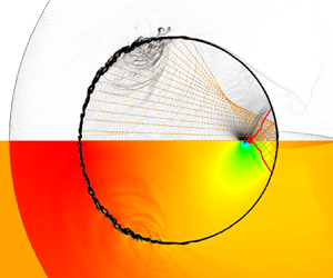
Figure 9 presents a comparison between the original model and the enhanced model alongside the numerical simulation results in two snapshots. The top section displays the numerical schlieren, while the theoretical analysis results from the original model (figures 9a,b) and the improved model (figures 9c,d) are shown below. In the theoretical analysis, the blue line inside the droplet denotes the location of the transmitted shock wave, derived from the disturbances’ ray ends. The blue line outside the droplet indicates the location of the incident shock wave. The red dashed line marks the current position of the starting disturbance, with the blue dashed line serving as an extension of the incident shock wave to highlight the inadequacy of solely employing it to trigger disturbances. The black circle signifies the droplet.
Comparison of numerical schlieren results (top part of image) and the theoretical results (bottom part) in the same instant, for  $M_s=4.8$, in (a,b) the original model and (c,d) the improved model. The blue line denotes the wave structure predicted by the theoretical model, and the red dashed line denotes the Mach stem location at the droplet surface. Times are (a,c)
 $t^*=0.630$, (b,d)
 $t^*=0.840$.

In figure 9, it is important to highlight that the current numerical schlieren results demonstrate the presence of the carbuncle phenomenon. This type of shock facility, aligned with the grid, can be addressed effectively by employing the approaches proposed by Fleischmann, Adami & Adams (Reference Fleischmann, Adami and Adams2020).
The incorporation of the Mach stem factor in the theoretical model markedly enhances its alignment with the numerical simulation results in figures 9(c,d). For instance, comparing figures 9(b,d), when using the incident shock wave as the disturbance initiation control factor in the previous model, the entire droplet exhibits disturbance at the selected moment, as depicted in the bottom of figure 9(b). In contrast, numerical simulation results in the top of figure 9(b) reveal some undisturbed points on the droplet. By employing the Mach stem as the governing factor in the improved model, illustrated in figure 9(d), the distribution state of the disturbance in the droplet at the chosen moment can be reconstructed accurately.
As shown in figure 10, the internal wave structures of the droplet at the time of the NPP obtained through the improved model closely align with the numerical simulation results. Here,  $\beta _{ref,k}$ represents the disturbance angle with
 $k$ reflections of the ray. Previous research (Wu et al. Reference Wu, Xiang and Wang2018; Biasiori-Poulanges & El-Rabii Reference Biasiori-Poulanges and El-Rabii2021; Xu et al. Reference Xu, Fan, Wu, Wen and Wang2023) indicates that the one-time reflected rays are responsible for generating negative pressure; therefore, other rays are not considered in this figure.
Comparison of the NPP point between (a,b) numerical schlieren and (c,d) theoretical analysis, for  $M_s=4.8$. The red dot is the NPP point obtained through numerical results, the blue line is the wavefront, and the yellow lines are the rays from disturbance inside the droplet. Only the rays within the angle
 $\beta _{ref,1}$ are drawn. Times are (a,c)
 $t^*=1.25$, (b,d)
 $t^*=1.14$.

Figures 10(a,c) depict a lower gas–liquid wave velocity ratio using air as the gas and  $n$-hexane as the liquid with
 $M_s=2.4$, while figures 10(b,d) display a higher gas–liquid wave velocity ratio with
 $M_s=4.8$. For instance, comparing figures 10(b,d), where figure 10(b) showcases the numerical simulation result of the numerical schlieren at the onset of the NPP, the theoretical result from the enhanced model at the same instance is illustrated in figure 10(d). In figure 10(d), the red dot signifies the NPP point's location derived from numerical simulation, while the blue line represents the shock envelope formed by each disturbance derived through the improved model. Notably, many rays that underwent once reflection converge at the NPP point's location. The agreement between the numerical simulation's NPP point's location and the theoretical analysis at the specific instant is apparent.
Although the focus of the expansion wave indeed induces pressure reduction and is closely linked to the NPP, the reasons for the divergence in the NPP point's location trend compared to that of Biasiori-Poulanges & El-Rabii (Reference Biasiori-Poulanges and El-Rabii2021) and Xu et al. (Reference Xu, Fan, Wu, Wen and Wang2023) remain unidentified.
5. Mechanism of the NPP formation
5.1. Difference between the NPP and focus points
Figure 5 illustrates that the NPP point's locations indicated by numerical simulations align with the theoretical results from Biasiori-Poulanges & El-Rabii (Reference Biasiori-Poulanges and El-Rabii2021) under low gas–liquid wave velocity ratios. However, a substantial variance emerges at higher gas–liquid wave velocity ratios. To analyse the reasons for this distinction, an improved theoretical model is employed to deduce the focus points at varying gas–liquid wave velocity ratios. This study defines the focus point obtained through theoretical analysis as the instant when the quantity of reflected waves traversing the central axis peaks within a specific range. At this moment, the location of the central axis wavefront is termed the focus point. As depicted in figure 11, the focus point is identified as the leftmost position of the wavefront (denoted by the blue line) within a range selected from one-fortieth to one-twentieth of the diameter, i.e.  $R = D_0/a$,
 $a\in [20,40]$.
The definition of focus in the selected region in the theoretical model.

The temporal evolution of the number of reflected waves (the time scale is equivalent to (4.10)) is portrayed in figure 12, with the dashed line indicating the instant when the NPP emerges, as determined by numerical simulations. For shock Mach number 2.4, regardless of the range size  $a$, the focusing time – marked by the maximum number of reflected waves – aligns closely with the NPP moment, suggesting congruence between the NPP and focus points in scenarios with lower wave velocity ratios. This finding supports the inference that the convergence of expansion waves can lead to pressure reduction under lower gas–liquid wave velocity ratios. Conversely, with shock wave Mach number 3.6, discrepancies between the focusing and NPP times grow; better alignment is observed with smaller ranges. At shock wave Mach numbers 5.4 and 8.4, significant deviations between focusing and NPP times occur across all selected range sizes, indicating non-coincidence of the NPP and focus points for elevated gas–liquid wave velocity ratios. Notably, at
 $M_{s}=8.4$, the ray promptly focuses near the right-hand wall of the droplet post-reflection, inducing a sudden shift in the focus degree (
 $k_{inc}/K$) from 0, as illustrated in figure 12(d). This observation demonstrates that the pressure decline at the focus point instigated by expansion waves fails to drive the pressure to its minimum, i.e. the NPP value.
Comparison of the NPP and focus points for three selected shock Mach numbers with  $n$-hexane as the liquid. The black dashed line is the instant when the NPP happens,
 $k_{inc}$ is the number of reflected waves in the selected region, and
 $K$ is the total number of reflected waves. Here, (a)
 $M_{s}=2.4$, (b)
 $M_{s}=3.6$, (c)
 $M_{s}=5.4$, (d)
 $M_{s}=8.4$.

Figure 13 contrasts the focus point locations derived from the improved theoretical model with the NPP point location from numerical simulations, the theoretical predictions by Biasiori-Poulanges & El-Rabii (Reference Biasiori-Poulanges and El-Rabii2021) and Xu et al. (Reference Xu, Fan, Wu, Wen and Wang2023), and the experimental findings of Sembian et al. (Reference Sembian, Liverts, Tillmark and Apazidis2016). The horizontal axis replaces the shock Mach number  $M_s$ with the gas–liquid wave velocity ratio
 $n$. It unveils that our improved theoretical forecast of the focus point's position aligns closely with the theoretical prediction by Biasiori-Poulanges & El-Rabii (Reference Biasiori-Poulanges and El-Rabii2021) at the low
 $n$ region.
Comparison of the focus point, the NPP point with water and  $n$-hexane as liquid phase, the theoretical results by Biasiori-Poulanges & El-Rabii (Reference Biasiori-Poulanges and El-Rabii2021), and the experimental results by Sembian et al. (Reference Sembian, Liverts, Tillmark and Apazidis2016).

Our focus locations, along with data from Biasiori-Poulanges & El-Rabii (Reference Biasiori-Poulanges and El-Rabii2021) and Biasiori-Poulanges & Schmidmayer (Reference Biasiori-Poulanges and Schmidmayer2023), exhibit a consistent downward trend with increasing gas–liquid wave velocity ratios. Observably, under lower gas–liquid wave velocity ratios, the NPP point lies between our focus spot and the Biasiori-Poulanges & El-Rabii (Reference Biasiori-Poulanges and El-Rabii2021) estimate, emphasizing its dependence solely on the gas–liquid wave velocity ratio rather than the liquid phase (water or  $n$-hexane) selected. As the gas–liquid wave velocity ratio escalates, disparities between focus point and NPP point's location emerge. High gas–liquid wave velocity ratios prompt numerical simulations to revert to a constant NPP point's location, aligning with the observations of Sembian et al. (Reference Sembian, Liverts, Tillmark and Apazidis2016).
In conclusion, the convergence of expansion waves contributes to pressure reduction at lower gas–liquid wave velocity ratios. However, at elevated gas–liquid wave velocity ratios, the pressure decrease arising from the expansion wave's focus point fails to reach the minimum necessary to designate this spot as an NPP point. Understanding the mechanism behind the generation of minimum pressure at NPP points entails comprehensive scrutiny of pressure-altering factors beyond solely expansion waves at the NPP and focus points.
5.2. Factors of the pressure variation
Initially, the pressure variation within the droplet during the early stages of shock–droplet interaction is categorized into four phases: the shock wave effect, relaxation effect, fluctuation effect and expansion wave effect, as illustrated in figure 14. As the transmitted wave traverses a point inside the droplet, for example, slightly to the left of the origin at  $-D_{0}/8$, the pressure sharply escalates at that specific location, as observed in the studies by Sembian et al. (Reference Sembian, Liverts, Tillmark and Apazidis2016), Biasiori-Poulanges & El-Rabii (Reference Biasiori-Poulanges and El-Rabii2021), Xu et al. (Reference Xu, Fan, Wu, Wen and Wang2023) and Xiang & Wang (Reference Xiang and Wang2017). Subsequently, owing to uneven pressure distribution within the droplet, this point gradually aligns with the neighbouring pressure, characterizing what we term the relaxation effect in this investigation.
The typical variation of pressure and its classification at point  $(-D_{0}/8, 0)$ inside the droplet.

Demonstrated in figure 15, the fluctuation effect arises from sustained high pressure on the droplet's upstream side, exemplified by  $M_s=2.4$ and 4.8 for low and high gas–liquid wave velocity ratios, respectively. Following the interaction of the external incident shock wave with the droplet, a region of heightened pressure forms diametrically opposite to the incident direction, inducing periodic pressure surges downstream, particularly at the droplet's centre. This fluctuation phenomenon is also noted in the experimental studies of Sembian et al. (Reference Sembian, Liverts, Tillmark and Apazidis2016). In the research by Schmidmayer & Biasiori-Poulanges (Reference Schmidmayer and Biasiori-Poulanges2023), the existence of the fluctuation effect is observable irrespective of whether the droplets are cylindrical or spherical.
Fluctuation effect in (a) low wave velocity ratio ( $M_s=2.4$) and (b) high wave velocity ratio (
 $M_s=4.$). The numerical schlieren is shown in the upper part of the image, and the pressure contour is shown in the lower part.

Nevertheless, the fluctuation effect is relatively minor in contrast to the impact of the shock wave. Subsequently, reaching this point, the expansion wave triggers a substantial pressure decrease. What follows is the natural evolution, encompassing fluctuation pressure influences, eventually stabilizing the pressure from its negative peak value. This marks the completion of a cycle. When the expansion wave strikes the wall edge and reflects, the subsequent traversal through that point initializes the ensuing cycle.
Figure 16 provides a depiction of the pressure distribution over time at various points along the central axis at different shock Mach numbers. Each selected point experiences the four delineated processes before the second convergence of the wave system: shock effect, fluctuation effect, relaxation effect and expansion wave effect. Notably, in figure 16(a), as the point nears the droplet's downstream side, the pressure increment from the shock wave's impact diminishes. Conversely, with an escalation in the shock Mach number, as demonstrated in figure 16(d), when the point approaches the droplet's downstream region, the pressure surge induced by the shock wave intensifies considerably.
Temporal pressure variation at different points ( $x=-D_{0}/4$,
 $-D_{0}/8$, 0,
 $D_{0}/8$,
 $D_{0}/4$, NPP point, focus point) in the
 $n$-hexane droplet at different cases, with (a)
 $M_s=2.4$, (b)
 $M_s=4.2$, (c)
 $M_s=4.8$, (d)
 $M_s=5.4$.

5.2.1. Shock effect
The shock wave effect phenomenon can be elucidated through theoretical analysis models to derive the internal wave system structure corresponding to the scenarios depicted in figures 16(a,d). In figure 17, two observation points are selected,  $-D_{0}/4$ and
 $D_{0}/4$ from the droplet's origin, to exemplify the comparison between shock Mach numbers 2.4 and 5.4. The internal wave structure is illustrated when the ray from the droplet's left pole reaches the observation point. For a lower gas–liquid wave velocity ratio (figures 17a,b), the rays emitted from the disturbed part of the droplet, impacting the envelope surface of the internal waves (now a transmitted wave), exhibit an outward propagation angle.
Theoretical analysis of shock effect at the points (a,c)  $x=-D_{0}/4$, (b,d)
 $x=D_{0}/4$, with shock Mach numbers (a,b)
 $M_s=2.4$, (c,d)
 $M_s=5.4$.

Consequently, the envelope surface shows a convex shape, termed diverging cases by Boyd & Jarrahbashi (Reference Boyd and Jarrahbashi2021). Since the selected points in figure 16 lie on the central axis, moving downstream results in the surrounding rays propagating outwards, gradually moving away from the central axis, reducing the impact from the rays. Hence in instances of lower gas–liquid wave velocity ratios, as depicted in figure 16(a), the pressure increase caused by the shock wave effect decreases as the point moves closer to the downstream wall of the droplet.
Conversely, when considering higher gas–liquid wave velocity ratios (figures 17c,d), the inward propagation angle of emitted radiation from the disturbance creates a concave shape on the envelope surface, termed converging cases by Boyd & Jarrahbashi (Reference Boyd and Jarrahbashi2021). As the observation point shifts to the right, the influence of each ray intensifies. Consequently, under a high gas–liquid wave velocity ratio illustrated in figure 16(d), points near the downstream wall experience a more pronounced pressure increase due to the shock wave effect.
5.2.2. Fluctuation effect
Observing figure 15 reveals that the source of fluctuation is the high-pressure region upstream of the droplet. Examination of figure 16 shows that when focusing on a specific shock Mach number, the amplitude of pressure fluctuations caused by the fluctuation effect increases as the chosen point approaches the high-pressure region near the upstream wall. The shorter propagation distance and weaker attenuation of high-pressure compression waves near the left point lead to a longer and stronger fluctuation effect due to the time gap between the shock wave and reflected expansion wave effects. Therefore, if the relaxation effect remains constant, then the point being closer to the upstream wall results in a lower pressure drop caused by the combined effects of fluctuation and relaxation at that specific point. Conversely, distancing the selected point from the high-pressure region of the upstream wall shortens the duration and intensity of experienced fluctuation effects, leading to a more rapid decline in pressure.
In considering the phenomenon where pressure fluctuations are not observable following a sudden pressure drop due to the expansion wave effect on a droplet, we can explain that the fluctuation effect operates by periodically emitting compression waves near the droplet's upstream wall. These waves sweep across the chosen point, inducing a pressure increase. While the droplet undergoes a rapid decline, the selected point is within the expansion wave's influence. The downstream transmission of the fluctuation effect from the high-pressure zone upstream of the droplet does not directly impact the point because it first encounters the expanding wave. Consequently, during the period of pressure decline and recovery at the chosen point, significant fluctuations are not visually discernible.
With the same liquid phase, as the shock Mach number increases, the gas–liquid velocity ratio increases, and the pressure change caused by the fluctuation effect weakens relative to other factors. Notably in figure 16(d), the intensity of the fluctuation effect weakens in contrast to instances with lower gas–liquid wave velocity ratios, with noticeable pressure fluctuation changes limited to points near the high-pressure area of the droplet's upstream wall. Particularly for the point along the droplet's downstream wall, due to its distance from the source of fluctuation in the high-pressure region and exposure to expansion wave effects shortly after encountering shock waves, the impact of upstream fluctuation is constrained. This limitation occurs because the effect weakens over distance, and the barrier between shock and expansion waves prevents direct influence on the point, emphasizing that higher shock Mach numbers reveal fluctuation impacts only near the high-pressure source region.
5.2.3. Relaxation effect
The relaxation effect can be understood as a downward trend within the droplet when the internal point experiences relatively high pressure or an upward trend in the presence of lower pressure. Focusing on a single research point within the droplet, the initial exposure to a shock wave results in maximum pressure at that location. Given the high-pressure environment around the specific point, the relaxation effect prompts pressure reduction, counteracted intermittently by the upstream fluctuation effect that makes the pressure raise. In this scenario, the fluctuation effect impedes the relaxation effect's pressure reduction.
When the point inside the droplet is impacted by the reflected expansion wave, the pressure reaches a minimum value. The low pressure leads to a relatively small pressure at the specific point compared to other points, resulting in the relaxation effect acting as a pressure booster. At the same time, the fluctuation effect, affecting points significantly impacted by it, drives further pressure increase. Consequently, the fluctuation effect fosters the rise of the relaxation effect.
Upon reaching the maximum pressure at the discussed point, the opposing forces of relaxation (causing pressure reduction) and fluctuation (driving pressure elevation) come into play. During this phase, the rate of pressure decline slows down. Conversely, once the minimum pressure is reached at the discussed point, both effects contributing to pressure elevation align, resulting in a swifter increase in pressure. Thus in figure 16, the duration required for pressure to return from the maximum value to a steady state exceeds the time needed for the pressure to rise from the minimum value to equilibrium.
In scenarios where different points experience the same shock Mach number, such as the case under discussion, when points near the upstream of the droplet undergo the shock wave effects, the surrounding points often remain unaffected by the shock waves, maintaining extremely low pressure levels. This condition accentuates the pressure disparity, enhancing the impact of the relaxation effect significantly. In contrast, when the shock effects reach downstream points, the surrounding area typically sustains a high-pressure state, resulting in a diminished pressure gap and weaker relaxation effects.
In summary, prior to a pronounced decrease in pressure following the peak impact of the shock wave within the droplet, a comprehensive evaluation of the fluctuation and relaxation effects becomes imperative. During this phase, the pressure drop ( $\Delta P=\Delta P_{flu}-\Delta P_{rel}$) comes into focus. Comparing the upstream and downstream points, the fluctuation effect is more pronounced at the upstream location, with a longer duration of impact (
 $\Delta P_{flu}$ is larger). Additionally, owing to the heightened pressure discrepancy with neighbouring points, the relaxation effect is also more pronounced (
 $\Delta P_{rel}$ is larger). While the fluctuation effect drives pressure elevation, the relaxation effect leads to pressure reduction. Hence establishing the pressure differential between upstream and downstream points under the amalgamated influence of both effects proves challenging through simplistic reasoning.
Nevertheless, as depicted in figure 16(c), the analysis of several points at  ${x=-D_{0}/4}, {-D_{0}/8}, {0}, D_{0}/8, D_{0}/4$ indicates an upward trend in the combined impact of fluctuation and relaxation effects (pressure drop
 $\Delta P$) within the upstream section delineated by
 $x=D_{0}/4$ as the selected point progresses rightwards. That is, as the selected point shifts towards the right, the pressure significantly diminishes. Furthermore, from the comparison of
 $x=NPP , Focus$, it can be seen that as the discussed point shifts to the right, the pressure drop is smaller.
Therefore, it can be considered that at the right of a critical point, due to the rapid alternation of shock waves and expansion waves, the upstream high-pressure fluctuations cannot be directly contacted, and the fluctuation effect can be ignored. Despite this, the persistence of low pressure downstream maintains a pressure differential, sustaining the impact of the relaxation effect. At the right of the critical point, the upstream point has a stronger relaxation effect than the downstream point, and the fluctuation effect is ignored, resulting in a stronger pressure drop.
5.3. Decreasing pressure caused by the reflected expansion wave
In the preceding subsection, it was observed that the focus of the reflected expansion wave does not inevitably result in the formation of NPP points in high gas–liquid wave velocity ratios, thus suggesting that it may not be the cause of cavitation. Furthermore, it is proposed that during the initial stage of shock–droplet interaction, the pressure variation within the droplet can be delineated into four phases: shock wave effect, fluctuation effect, relaxation effect and expansion wave effect.
What follows first defines the pressure decrease contribution caused by expansion waves in the pressure variation curve,  $\Delta P_{exp}$, and compares it with the number of reflected waves obtained from the improved theoretical model. This comparison is employed to illustrate quantitatively that the pressure reduction attributed to reflected expansion waves constitutes just one component of the overall pressure decline. Noteworthy is the fact that focusing represents only the maximum pressure drop caused by the reflected expansion wave at that point, and it may not necessarily lead to the NPP considering the pressure variation with the four parts of the factors.
Upon scrutinizing the pressure trend depicted in figures 14 and 16, the straightforward approach to discern whether the pressure descent stems from the relaxation effect or the expansion wave is by evaluating its rate of decline. A prominent slope in the pressure trend indicates the impact of the expansion wave, as illustrated by the first-order derivative plot of pressure against time for the case  $M_s=4.2$ displayed in figure 18.
First derivative of pressure and the definition of decreasing pressure caused by a reflected expansion wave for  $M_s=4.2$.

After being subjected to the shock wave and increasing significantly, the pressure decreases at a relatively stable speed under the influence of relaxation and fluctuation. For a more refined differentiation between the effects of expansion waves and relaxation, this study introduces the definitions of the initiation time  $t_1$ and cessation time
 $t_3$ of expansion wave influence. Here, the initiation time marks the instance when the initial trough preceding the minimum value of the first pressure derivative (
 $t_2$) transpires. Conversely, the cessation time denotes the moment when the first derivative of pressure first attains zero subsequent to reaching its minimum (
 $t_2$). The pressure drop between
 $t_1$ and
 $t_3$ attributed to the reflection of expansion waves is denoted as
 $\Delta P_{exp}$.
In figure 19, the comparison between the pressure drop  $\Delta P_{exp}$ from reflected expansion waves at specific points and the total pressure drop
 $\Delta P_{total}$ from the maximum pressure post-shock wave to the minimum pressure post-expansion wave is depicted. The ratio of reflected waves
 $k_{inc}/K$ is illustrated as well. Here,
 $k_{inc}$ represents the reflected waves at the selected point, indicating the strength of focusing, while
 $K$ denotes the total number of waves, including those with multiple reflections or no reflection. Notably, as the point approaches the right-hand boundary of the droplet, both the number of reflected waves (
 $k_{inc}$) and the pressure drop from the expansion wave (
 $\Delta P_{exp}$) become more pronounced.
Reflected rays  $k_{inc}/K$ with different range
 $a$ (dashed lines), decreasing pressure caused by expansion wave
 $\Delta P_{exp}$ and total decreasing pressure
 $\Delta P_{total}$ (solid lines) at different cases, with (a)
 $M_s=2.4$, (b)
 $M_s=4.2$, (c)
 $M_s=4.8$, (d)
 $M_s=5.4$.

Particularly in figures 19(a,b), the variations in  $k_{inc}$ and
 $\Delta P_{exp}$ across all locations are closely aligned, suggesting that the reflected expansion wave significantly influences
 $\Delta P_{exp}$. In the study by Schmidmayer & Biasiori-Poulanges (Reference Schmidmayer and Biasiori-Poulanges2023), it is posited that the focus level of the reflected expansion wave becomes fixed once the shape of the transmitted wave and reflector is established, aligning with our finding that the reduction in pressure caused by the expansion wave (
 $\Delta P_{exp}$) and the focus level
 $k_{inc}/K$ exhibit parallel trends.
Nevertheless, the total pressure drop ( $\Delta P_{total}$) at the NPP point surpasses that at the focal point, notably with higher shock Mach numbers. Given the increased distance between the NPP and the droplet's right-hand boundary compared to the focus point, the NPP experiences extended durations of fluctuation and relaxation effects. This underscores the importance of considering all factors influencing pressure variations, particularly the impact of transmitted shock waves and relaxation effects when determining the NPP point's location. Consequently, the negative pressure recorded at the NPP is the most extreme within the droplet, indicating a heightened likelihood of cavitation occurrence.
In this section, focus is defined using the improved theoretical model, determining the proportion of reflected waves at points along the central axis of the droplet. Comparison between the focus from theoretical analysis and the NPP point from numerical simulation reveals a close alignment under low gas–liquid wave velocity ratios. However, at higher wave velocity ratios, the focus point shifts nearer to the droplet's downstream compared to the negative pressure point.
For the exploration of the phenomenon that the NPP value can still be reached when the number proportion of reflected waves is not the maximum, four factors are used to explain the total pressure variation in the shock–droplet interaction. Finally, by comparing the pressure decrease caused by the expansion wave ( $\Delta P_{exp}$) with the total pressure drop (
 $\Delta P_{total}$) and the number of reflected waves (
 $k_{inc}$), it is found that the number of reflected waves
 $k_{inc}$ affects the pressure drop caused by the expansion wave
 $\Delta P_{exp}$, and the
 $\Delta P_{exp}$ at the focus is indeed the largest among all points inside the droplet. However, the
 $\Delta P_{total}$ of the NPP point is the highest among the points inside the droplet, and the
 $\Delta P_{total}$ is the consequence of considering all the four factors. Hence integrating these four pressure variation elements results in a more pronounced negative pressure at the NPP point compared to the focus point.
6. Conclusion
This study explores the interaction between shock waves and droplets through high-fidelity simulations and an improved theoretical model. The results align well with recent findings for lower gas–liquid wave velocity ratios, indicating a consistent NPP point. However, for higher ratios, the NPP point's location tends to remain constant, deviating from the decreasing trend projected by Biasiori-Poulanges & El-Rabii (Reference Biasiori-Poulanges and El-Rabii2021) and Xu et al. (Reference Xu, Fan, Wu, Wen and Wang2023). To elucidate this phenomenon, the theoretical model is refined and applied, incorporating information on the Mach stem through ray-tracing methods.
The existing theoretical model is inadequate for scenarios with high gas–liquid wave velocity ratios. In instances with low ratios, the speed of the incident shock wave external to the droplet is slower than the transmitted shock wave within. The incident shock wave detaches from the envelope of the transmitted shock wave at the close time of the appearance of the Mach stem, leading to the neglect of the role of the Mach stem. In contrast, at higher ratios, the external wave velocity surpasses the internal transmission speed. After its appearance, the Mach stem constantly adheres to the boundary of the droplet, and exerts a continuous impact on the envelope inside the droplet. Hence the theoretical model is enhanced to encompass the Mach stem's role, ensuring its applicability across a broader range of gas–liquid wave velocity ratios.
The improved theoretical model is used to obtain the information of the focus point. It is found that it has the same decreasing trend as the expression of Biasiori-Poulanges & El-Rabii (Reference Biasiori-Poulanges and El-Rabii2021), but has a significant deviation from the NPP point location obtained by numerical simulation under high gas–liquid wave velocity ratios. Consequently, a distinction is proposed between the focus point, where the reflected expansion wave converges, and the NPP point, where the maximum negative pressure might induce cavitation in the initial stages of shock–droplet interaction.
The discussion further delves into the relationship between the convergence of reflected expansion waves and the emergence of the NPP point. The pressure variation at a point within the droplet is attributed to four key factors, namely, the pressure rise caused by the shock wave, the relaxation effect that makes the pressure tend to be constant, the pulse pressure from the high-pressure part upstream of the droplet to increase the pressure intermittently, and the pressure drop caused by the expansion wave. Comparisons are made among the proportion of reflected waves ( $k_{inc}$), the pressure drop from expansion waves (
 $\Delta P_{exp}$), and the overall pressure drop (
 $\Delta P_{total}$). Results illustrate that across various shock Mach number scenarios, as the distance between the point on the central axis and the right-hand boundary of the droplet decreases, both the number of reflected wave convergences (
 $k_{inc}$) and the pressure decrease from expansion waves (
 $\Delta P_{exp}$) increase, signifying a direct correlation between the two. Nonetheless, the total pressure drop at the NPP point surpasses that at the focus point. The NPP, which potentially triggers cavitation, shows the most substantial pressure drop, while the expansion wave focus contributes only partially. Any occurrence of NPP necessitates a meticulous consideration of these four influential factors.
This research employs a five-equation model; however, the absence of phase transition renders the cavitation process invisible. Future endeavours should focus on validating the probable cavitation sites identified in this study through numerical methods incorporating phase transitions. Subsequently, extensive investigations are warranted to elucidate the manifestation of the four pressure variation factors.
Funding
This research is financially supported by the National Natural Science Foundation of China (no. 52276151), the Talent Recruitment Project of Guangdong (2021QN020231), the Guangdong Basic and Applied Basic Research Foundation (2023A1515012990), and the Foundation of Shenzhen Science and Technology Committee (GXWD20231130201948001).
Declaration of interests
The authors report no conflict of interest.
Appendix A
In this appendix, we analyse the impact of grid resolution on the locations of the NPP, a crucial factor discussed in § 3. Figure 20 displays the NPP point's locations for different gas–liquid wave velocity ratios ( $n$): small
 $M_s = 2.4$ (water), moderate
 $M_s = 4.8$ (
 $n$-hexane), and large
 ${M_s = 8.4}$ (
 $n$-hexane). The grid cell per diameter (
 $N_D$) values used are 100, 200, 400 and 800, respectively. We also consider
 $N_D$ = 1600 specifically for the case
 $M_s = 2.4$ due to its lack of convergence trend at the aforementioned grid resolution.
The effect of grid resolution on the NPP point's locations with  $N_D = 100$, 200, 400, 800, 1600. The NPP point with water and
 $n$-hexane as liquid phase with
 $N_D = 800$, the theoretical results by Biasiori-Poulanges & El-Rabii (Reference Biasiori-Poulanges and El-Rabii2021), and the experimental results by Sembian et al. (Reference Sembian, Liverts, Tillmark and Apazidis2016), are also shown for comparison.

From figure 20, it is evident that the NPP point's location remains similar for grid resolutions 800 and 1600 in the case  $M_s = 2.4$. Furthermore, for
 $M_s = 4.8$ (
 $n$-hexane) and
 $M_s = 8.4$ (
 $n$-hexane), the NPP point's location converges at
 $N_D = 400$ and 800. Hence we conclude that
 $N_D = 800$ provides sufficient resolution for determining the NPP point's location. Notably, recent research by Schmidmayer & Biasiori-Poulanges (Reference Schmidmayer and Biasiori-Poulanges2023) employed
 $N_D = 400$, Biasiori-Poulanges & Schmidmayer (Reference Biasiori-Poulanges and Schmidmayer2023) used
 $N_D = 800$, and Xu et al. (Reference Xu, Fan, Wu, Wen and Wang2023) employed
 $N_D = 800$. Xu et al. (Reference Xu, Fan, Wu, Wen and Wang2023) investigated shock–water column interaction and found no notable differences among
 $N_D = 800$, 1200 and 1600. Therefore, our chosen mesh resolution aligns with these studies, and we opt for
 $N_D = 800$ for the present investigation.
Next, we explore the impact of grid resolution on the temporal evolution of pressure, a significant aspect discussed in § 5. Figure 21 illustrates the temporal variation of pressure at position  $x =D_0/4$ for
 $N_D$ values of 100, 200, 400, 800, and 1600, respectively. As the resolution increases, we observe that the overall temporal trend and fluctuations in pressure remain almost unchanged. The moment of minimum pressure, occurring at
 $t^\star = 1.28$, remains consistent across all resolutions. However, it is important to note that the specific pressure values are not the focus of our study as we do not fully resolve the cavitation process. Based on these observations, we can conclude that the grid resolution of
 $N_D = 800$ accurately captures the temporal evolution of
Temporal evolution of pressure at  $x =D_0/4$ with different grid resolutions (
 $M_s = 2.4$,
 $N_D = 100$, 200, 400, 800, 1600).

Appendix B
The difference between the model of Kapila et al. (Reference Kapila, Menikoff, Bdzil, Son and Stewart2000) and the model of Allaire, Clerc & Kokh (Reference Allaire, Clerc and Kokh2002) lies in whether the convection equation for volume fraction has the expansion term  $K\,\boldsymbol {\nabla } \boldsymbol {\cdot } u$. The convection equation for volume fraction in the model of Kapila et al. (Reference Kapila, Menikoff, Bdzil, Son and Stewart2000) is
 \begin{equation} \frac{\partial{\alpha _1}} {\partial{t}} +{\boldsymbol{u}}\boldsymbol{\cdot}\boldsymbol{\nabla}\alpha _1=K\,\boldsymbol{\nabla} \boldsymbol{\cdot} u, \end{equation}
where the  $K$ term represents expansion and compression in mixture regions. For a two-component model, it is expressed as
 \begin{equation} K=\frac{\rho_2c_2^2-\rho_1c_1^2}{\dfrac{\rho_2c_2^2}{\alpha_2}+\dfrac{\rho_1c_1^2}{\alpha_1}}, \end{equation}
where  $\rho$,
 $c$ and
 $\alpha$ represent the density, sound speed and volume fraction of the mixture region, respectively. Subscripts represent different components.
To evaluate the expansion term  $K\,\boldsymbol {\nabla } \boldsymbol {\cdot } u$, we conducted numerical simulations both with and without the
 $K$ term. The results are depicted in figure 22.
The pressure variation of the internal points of a droplet with or without the  $K$ term.

In general, the comparative analysis reveals that the  $K$ term has minimal impact on the initial stages of the shock–droplet interaction investigated in our study. Figure 22 illustrates that when the model incorporates the
 $K$ term, the pressure surge induced by shock waves is enhanced, while the fluctuation effect is reduced compared to the model without the
 $K$ term. However, there is no notable disparity in the minimum pressure, indicating that the NPP point remains unchanged. Additionally, the pressure trends remain consistent, encompassing the effects of shock waves, wave propagation, relaxation and expansion waves as discussed in the mechanism analysis.
Moreover, since our research does not specifically address the cavitation process, gas expansion is not considered. As demonstrated by Schmidmayer, Bryngelson & Colonius (Reference Schmidmayer, Bryngelson and Colonius2020), the non-conservative nature of the  $K$ term can lead to numerical instabilities in regions with intense compression or expansion in mixtures. To ensure the stability of our simulation, we opt to disregard the expansion term.
Appendix C
The SGEOS parameters for water were selected based on the work of Gojani et al. (Reference Gojani, Ohtani, Takayama and Hosseini2016) and Meng & Colonius (Reference Meng and Colonius2018), specifically  $\gamma = 6.12$ and
 ${\rm \pi} _\infty = 3.43\times 10^8$. These parameters have been utilized widely in the study of shock–droplet interaction, as indicated by Coralic (Reference Colonius and Coralic2014), Meng & Colonius (Reference Meng and Colonius2015) and Dorschner et al. (Reference Dorschner, Biasiori-Poulanges, Schmidmayer, El-Rabii and Colonius2020).
Furthermore, the SGEOS parameters for water have been documented or derived from various experimental data sources, such as Marsh (Reference Marsh1980) and Cocchi, Saurel & Loraud (Reference Cocchi, Saurel and Loraud1996). Three sets of distinct experimental data were employed to fit the SGEOS parameters, including data from Gojani et al. (Reference Gojani, Ohtani, Takayama and Hosseini2016) used in the simulations, as well as data from Marsh (Reference Marsh1980) and Cocchi et al. (Reference Cocchi, Saurel and Loraud1996). The corresponding parameters obtained from these sources are presented in table 3.
The SGEOS parameters in different experimental data sets.

Figure 23 displays the NPP profiles generated using different SGEOS parameters. It is evident that the profiles derived from Gojani et al. (Reference Gojani, Ohtani, Takayama and Hosseini2016) and Marsh (Reference Marsh1980) resemble each other closely, suggesting the validity of the SGEOS parameters obtained from these experimental data sources. Moreover, when comparing the case ‘Marsh (Reference Marsh1980)  $M_s = 1$’ with ‘Marsh (Reference Marsh1980)
 $M_s = 2$’, it is observed that the value of
 $M_s$ has minimal impact on the NPP profiles when the slope
 $\alpha$ and intercept
 $c_0$ from the experimental data remain constant. Therefore, the experimental data from Marsh (Reference Marsh1980) can also be considered a reliable source for obtaining the SGEOS parameters.
The NPP profiles using different SGEOS parameters.

As for  $n$-hexane, we determined its SGEOS parameters based on the experiments conducted by Marsh (Reference Marsh1980) due to the limited availability of experimental sources. The expressions used to derive the SGEOS parameters were based on Johnsen (Reference Johnsen2008):
 $$\begin{gather} \gamma=2\alpha\left(1+\frac1{M_s}\right)-1, \end{gather}$$
 $$\begin{gather}{\rm \pi} _\infty=\frac{\rho_oc_o^2}\gamma-p_o, \end{gather}$$
where  $\alpha$ and
 $c_o$ are the slope and intercept of the fitted line, respectively,
 $M_s$ is the shock Mach number,
 $p_o$ is taken to be the ambient atmospheric pressure, and
 $\gamma$ and
 ${\rm \pi} _{\infty }$ are the SGEOS parameters. The slope of the fitted line
 $\alpha$ obtained through the Marsh (Reference Marsh1980) experiment is 1.5985, and the intercept
 $c_o$ is 1090 m s
 $^{-1}$. By substituting into the above equation, we can obtain
 $\gamma = 5.394$ and
 ${\rm \pi} _\infty = 1.45\times 10^8$ for
 $n$-hexane.
Appendix D
In Xu et al. (Reference Xu, Fan, Wu, Wen and Wang2023), the transmitted shock wave speed  $u_l$ is obtained following the Rankine–Hugoniot relation (Haller et al. Reference Haller, Ventikos, Poulikakos and Monkewitz2002, Reference Haller, Poulikakos, Ventikos and Monkewitz2003; Nagayama et al. Reference Nagayama, Mori, Motegi and Nakahara2006) and can be expressed as
 \begin{equation} u_l=\frac{\gamma_l+1}{4}\left(u_p+\sqrt{u_p^2+16\,\frac{1}{(\gamma_l+1)^2}\,c_l^2}\right), \end{equation}
where  $\gamma _l$ represents the specific heat ratio of liquid (6.12 for water, and 5.39 for
 $n$-hexane),
 $c_l$ represents the sound speed of the liquid at the initial state (1450 m s
 $^{-1}$ for water, and 1090 m s
 $^{-1}$ for
 $n$-hexane), and
 $u_p$ represents the velocity of the liquid inside the water column behind the transmitted shock wave.
The shock wave Mach number discussed in the study by Xu et al. (Reference Xu, Fan, Wu, Wen and Wang2023) is 2.4, which indicates a low shock intensity. Consequently, the propagation velocity  $u_l$ of the wave configurations inside the droplet can be approximated as
 $c_l$, where
 $c_l$ represents the wave velocity. In our research, which focuses on high shock intensities, we first evaluate the velocity
 $u_p$ using our simulation results. We determine the maximum velocity of the liquid inside the water column behind the transmitted shock wave at
 $x =D_0/8$ as
 $u_p$. The values of
 $u_p$ for both phases in all cases are presented in table 4.
The velocity of the liquid inside the water column behind the transmitted shock wave  $u_p$.

Next, we conduct curve fitting to establish a relationship between  $u_p$ and
 $M_s$, as shown in figure 24. By incorporating
 $u_p(M_s)$ into (D1) we calculate the wave velocity
 $u_l(M_s)$. We then apply this wave velocity to our theoretical analysis model to determine the focus point. In figure 25, we compare our current findings with previous results that utilized a constant wave velocity. Notably, when selecting
 $u_l = u_l(M_s)$, we also update the corresponding gas–liquid wave velocity ratio
 $n$. It is evident from figure 25 that regardless of whether a constant
 $c_l$ or the realistic
 $u_l(M_s)$ is employed as
 $u_l$, and regardless of whether the liquid phase is
 $n$-hexane or water, the position of the focus point follows a universal line that is solely dependent on the gas–liquid wave velocity ratio
 $n$.
The fitting relationship between  $u_p$ and
 $M_s$.

The location of the focus point with different  $u_l$ calculations.

Therefore, as the Mach number of the shock wave increases, any increase in liquid compressibility resulting in a higher sound velocity does not impact the focusing of the reflected expansion wave.
Appendix E
We compare the trajectory of the Mach stem using different mesh resolutions, as illustrated in figure 26. There are no significant differences in the trajectory of the Mach stem when varying the mesh resolution.
Comparison of the trajectory of the Mach stem with different mesh resolutions.

Next, we analyse the impact of different fitting functions. The original curve fitting for the Mach stem trajectory is depicted in figure 8(b). Notably, the Mach stem trajectory corresponding to  $M_s=8.4$ in figure 8(b) appears to have the most downward offset compared to the current fitted curve. We perform curve fitting for the Mach stem trajectory
 $M_s=8.4$, and compare it with the original fitting in figure 27. The two curves exhibit minimal discrepancies.
Comparison of different Mach stem fitting curves.

To assess the influence of the fitting function on theoretical analysis, we quantitatively compare the focus point values. The fitting formula  $\beta (t_M)$ is used to obtain its inverse function
 $t_M(\beta )$. Subsequently, based on (4.6), we calculate the length of each ray at the current time. The meaning of
 $\beta (t_M)$ is that at time
 $t_M$, the Mach stem, which affects the generation of rays, has reached the
 $\beta$ location. Conversely, the meaning of
 $t_M(\beta )$ is the time required for the Mach stem to reach the
 $\beta$ location. Rays at the
 $\beta$ location will commence generation upon the arrival of the Mach stem. Consequently, the selection of fitting formulas inevitably influences the results of the theoretical analysis. To illustrate this effect, we compare the focus values using different fitting curves, as depicted in figure 27. The obtained expression,
 $\beta =f(T_M)=-9\times {10}^{-5}(T_M)^2+0.2442T_M+27.132$, is used to replace (4.11) for the liquid phase. Theoretical analysis is then conducted to determine the focus for cases with
 $M_s=5.4$ and 7.8, with water as the liquid phase. The comparison is provided in table 5, revealing that the focus point values exhibit negligible differences across different fitting curves.
Focus predicted by different fitting expressions.



