1 Introduction
Extensive experimental and numerical research has been conducted to systematically study the transition of laminar to turbulent flow in the wake of circular cylinders (Roshko Reference Roshko1954; Hammache & Gharib Reference Hammache and Gharib1991; Karniadakis & Triantafyllou Reference Karniadakis and Triantafyllou1992; Barkley & Henderson Reference Barkley and Henderson1996; Thompson, Hourigan & Sheridan Reference Thompson, Hourigan and Sheridan1996; Zhao et al.
Reference Zhao, Thapa, Cheng and Zhou2013). Williamson (Reference Williamson1996) presented a comprehensive review on steady and unsteady flow regimes in the wake of a circular cylinder as a function of Reynolds number. It has been well established that as the Reynolds number is increased beyond
 $Re=47$
, flow in the wake of a circular cylinder becomes unsteady, characterized by periodic shedding of vortices from the two sides of the cylinder, forming the so-called von Kármán vortex street. The wake flow remains two-dimensional until the Reynolds number exceeds approximately
 $Re=190$
, where the primary vortices in the wake of the cylinder begin to deform into secondary three-dimensional vortices (Brede, Eckelmann & Rockwell Reference Brede, Eckelmann and Rockwell1996). These secondary vortices in the wake of the cylinder have a spanwise wavelength of around 3–4 cylinder diameters and are called mode A vortex shedding (Williamson & Roshko Reference Williamson and Roshko1988). As the Reynolds number is further increased to above
 $Re=230{-}240$
, the three-dimensional wake flow transitions in to mode B, which is dominated by streamwise vortex pairs distributed along the cylinder span with a spacing of approximately one cylinder diameter (Wu et al.
Reference Wu, Sheridan, Welsh, Hourigan and Thompson1994, Reference Wu, Sheridan, Hourigan and Soria1996a
,Reference Wu, Sheridan, Welsh and Hourigan
b
).
It is well known that if the cylinder rotates around its axis, the asymmetric wake flow leads to a net lift force acting on the cylinder due to the Magnus effect (Prandtl Reference Prandtl1926). In addition to the Reynolds number, the rotation rate
 $\unicode[STIX]{x1D6FC}$
, defined as the ratio of the rotational speed of the cylinder surface to the free-stream velocity, has a significant effect on the flow past a rotating cylinder (Chang & Chern Reference Chang and Chern1991). It was found that at low rotation rates (
 $\unicode[STIX]{x1D6FC}<2$
), the vortex street in the wake of the cylinder is similar to the von Kármán vortex street and the vortex shedding is called mode I shedding (Stojković, Breuer & Durst Reference Stojković, Breuer and Durst2002; Pralits, Brandt & Giannetti Reference Pralits, Brandt and Giannetti2010). As the rotation rate
 $\unicode[STIX]{x1D6FC}$
is increased beyond 2, the vortex shedding in the wake of a rotating cylinder is fully suppressed (Diaz et al.
Reference Diaz, Gavalda, Kawall, Keffer and Giralt1983; Badr et al.
Reference Badr, Coutanceau, Dennis and Menard1990; Chew, Cheng & Luo Reference Chew, Cheng and Luo1995; Chou Reference Chou2000). Early studies on flow past a rotating cylinder were focused on the laminar flow regime (Tang & Ingham Reference Tang and Ingham1991). Kang, Choi & Lee (Reference Kang, Choi and Lee1999) investigated laminar flow past a rotating circular cylinder through numerical simulations and found that the critical
 $\unicode[STIX]{x1D6FC}$
above which there was no vortex shedding increases with the increase in Reynolds number. The critical rotation rates for
 $Re=60$
, 100 and 160 were found to be approximately 1.4, 1.8 and 1.9, respectively. Moreover, for rotation rates lower than the critical rotation rate, the Strouhal number remains nearly independent of the rotation rate.
In addition to the mode I vortex shedding, similar to that observed in the wake of a non-rotating cylinder, Stojković et al. (Reference Stojković, Breuer and Durst2002) were the first to find the existence of a second vortex shedding mode, referred to as mode II shedding, in the range of rotation rate of
 $4.8\leqslant \unicode[STIX]{x1D6FC}\leqslant 5.15$
at
 $Re=100$
. The two-dimensional numerical study of Stojković et al. (Reference Stojković, Schön, Breuer and Durst2003) further confirmed the existence of this second mode in the Reynolds number range
 $60\leqslant Re\leqslant 200$
. The second vortex shedding mode, also known as the secondary instability regime, occurs over a narrow range of high rotation rate. In this regime, single-sided vortex shedding occurs with a period much longer than the vortex shedding period in mode I vortex shedding (Pralits et al.
Reference Pralits, Brandt and Giannetti2010). The oscillation amplitude of the lift coefficient increases considerably in the secondary instability regime. Mittal & Kumar (Reference Mittal and Kumar2003) and Lu et al. (Reference Lu, Qin, Teng and Li2011) found that, for
 $Re=200$
, the wake flow remains stable for rotation rates in the range of
 $1.91\leqslant \unicode[STIX]{x1D6FC}\leqslant 4.34$
, loses its stability at
 $\unicode[STIX]{x1D6FC}\approx 4.35$
and becomes stable again as the rotation rate exceeds 4.8. El Akoury et al. (Reference El Akoury, Braza, Perrin, Harran and Hoara2008) conducted detailed two-dimensional numerical simulations for
 $Re\leqslant 500$
and
 $\unicode[STIX]{x1D6FC}\leqslant 6$
in which he concluded that the effect of higher Reynolds number was to bring about early transition to secondary instability. Lam (Reference Lam2009) studied flow past a rotating cylinder at
 $Re=3600{-}5000$
and
 $\unicode[STIX]{x1D6FC}\leqslant 2.5$
using flow visualization and particle image velocimetry (PIV) measurements. It was found that the wake became increasingly narrow and deflected sideways with increasing cylinder rotation rate and the formation length of the vortices decreased with increasing
 $\unicode[STIX]{x1D6FC}$
, leading to a slight increase in the vortex shedding frequency.
A limited number of studies have been carried out to investigate the development of three-dimensionality in the wake of rotating cylinders. El Akoury et al. (Reference El Akoury, Braza, Perrin, Harran and Hoara2008), in addition to two-dimensional numerical simulations, performed three-dimensional direct numerical simulations (DNS) at low rotation rates of
 $\unicode[STIX]{x1D6FC}\leqslant 1.5$
. They found that the three-dimensional flow at higher rotation rate became increasingly complex and the critical Reynolds number for two- to three-dimensional wake flow transition moved to a higher value. At
 $\unicode[STIX]{x1D6FC}=0.5$
, the critical Reynolds number was found to be around 220, and the flow remained two-dimensional at
 $\unicode[STIX]{x1D6FC}=1.5$
and
 $Re=200$
. Mittal (Reference Mittal2004) performed numerical simulations to study the three-dimensionality of flow past a rotating cylinder at
 $Re=200$
and a wide range of
 $\unicode[STIX]{x1D6FC}$
from 0 to 5. It was found that centrifugal instabilities exist along the entire span for the rotation rate
 $\unicode[STIX]{x1D6FC}$
of 5. Tokumaru & Dimitakis (Reference Tokumaru and Dimitakis1993) investigated the influence of the cylinder length-to-diameter aspect ratio on the mean lift coefficient at
 $Re=3800$
and found that the aspect ratio affects the lift coefficient if it is too small.
Rao et al. (Reference Rao, Leontini, Thompson and Hourigan2013a
,Reference Rao, Leontini, Thompson and Hourigan
b
) used linear stability analysis to study two- to three-dimensional transition of wake flow past a rotating cylinder at Reynolds numbers less than 400 and rotation rate
 $\unicode[STIX]{x1D6FC}\leqslant 7$
. They observed that the three-dimensionality in the wake of a rotating cylinder resembled its stationary counterpart for
 $\unicode[STIX]{x1D6FC}\leqslant 1$
. Five unsteady three-dimensional modes were found in the mode I shedding regime, and four three-dimensional modes were observed in the steady regimes of flow for
 $\unicode[STIX]{x1D6FC}>2$
. The experimentally observed flow modes by Radi et al. (Reference Radi, Thompson, Rao, Hourigan and Sheridan2013) were in excellent agreement with those observed in the numerical simulations. Later, Navrose, Meena & Mittal (Reference Meena and Mittal2015) performed a detailed linear stability analysis at
 $200\leqslant Re\leqslant 350$
to study the steady and unsteady modes associated with mode I shedding and mode II shedding for a range of
 $\unicode[STIX]{x1D6FC}\leqslant 5$
. They found that the spanwise length of the cylinder has a considerable effect on the occurrence of modes. It was further observed that mode E was the first unsteady mode associated with the start of the mode II shedding and as the rotation rate was further increased to
 $\unicode[STIX]{x1D6FC}=3.5$
and
 $Re=200$
, a combination of modes E and H was observed, making the wake flow complex.
Based on the above discussion, it can be concluded that there are not enough studies through DNS on the flow classification and vortex flow dynamics of a high-speed rotating circular cylinder. Although Navrose et al. (Reference Meena and Mittal2015) conducted an in-depth linear stability analysis of the flow around a rotating cylinder to study different flow modes, the formation physics of different flow structures as a function of rotation rate needs to be further discovered for accurate flow classification and an understanding of the vortex flow dynamics.
In light of the above discussion, the aim of the current study is to investigate the effect of a high rotation rate on the wake flow past a rotating circular cylinder for Reynolds numbers in the laminar and turbulent flow regimes. To achieve this, wake flow structures are analysed to identify the transition between different flow regimes both as a function of rotation rate and Reynolds number; the identified flow regimes are mapped on an
 $\unicode[STIX]{x1D6FC}$
-
 $Re$
map; the vortex generation and motion mechanism along the surface of the cylinder are analysed in detail to understand the flow dynamics of a rotating cylinder at high rotation speed; and the effects of different flow regimes on the fluid forces of the cylinder are discussed. Numerical simulations are performed for a range of rotation rates from 1.6 to 6 with an increment of 0.2 and five Reynolds numbers of
 $Re=100$
, 150, 200, 250 and 500. The length of the circular cylinder in the present study is 6.4 cylinder diameters.
The rest of the paper is arranged as follows: in § 2, the governing equations and the numerical model used in this study are presented. In § 3.1, a detailed analysis of the flow structures for
 $Re=200$
is presented to identify the different flow regimes as a function of rotation rate; the identified flow regimes for all the rotation rates and Reynolds numbers are mapped on an
 $\unicode[STIX]{x1D6FC}$
-
 $Re$
map. Next, the formation dynamics of flow structures at different flow regimes for
 $Re=200$
is studied in detail. In § 3.2, the detailed flow structures for
 $Re=100$
, 200, 250 and 500 are presented and classified as a function of rotation rate. In § 3.3, time histories of the lift coefficient for
 $Re=200$
and a range of rotation rates are presented, and comparison is made with the previous results. This is followed by a discussion on the plots of the lift and drag coefficients as a function of rotation rate for a range of Reynolds numbers. Finally, conclusions are drawn in § 4.
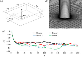
(a) Flow around a rotating cylinder; (b) computational mesh near one end of the cylinder; (c) comparison between the lift coefficients calculated from different meshes. The properties of different meshes are listed in table 1.

2 Numerical method
Figure 1 shows a sketch of the computational domain for simulating flow around a rotating cylinder. The cylinder rotates with an angular rotational speed of
 $\unicode[STIX]{x1D714}$
. The non-dimensional rotation rate
 $\unicode[STIX]{x1D6FC}$
is defined as
 $\unicode[STIX]{x1D6FC}=\unicode[STIX]{x1D714}D/(2U)$
where
 $D$
is the diameter of the cylinder and
 $U$
is the incoming flow velocity. In the numerical simulation, the computational domain size in the axial direction of the cylinder is large enough to minimize the influence of domain size effect. It was reported that a cylinder length of
 $2D$
is enough for accurately predicting the fluid forces at
 $Re=1000$
(Lei, Cheng & Kavanagh Reference Lei, Cheng and Kavanagh2001). Gioria et al. (Reference Gioria, Meneghini, Aranha, Barbeiro and Carmo2011) investigated the effects of computational domain size in the spanwise direction on the flow around a circular cylinder at
 $Re=400$
and reported that the three-dimensional flow can be reasonably represented if
 $L$
exceeds 6 diameters. In this study, the length-to-diameter ratio of the cylinder is 6.4. The computational domain size is
 $50D$
in the flow direction and
 $40D$
in the cross-flow direction.
The governing equations for simulating the flow are the incompressible continuity and Navier–Stokes (N–S) equations. Direct numerical simulations through solving the N–S equations are still challenging for complex flows with large Reynolds numbers (Borazjani, Ge & Sotiropoulos Reference Borazjani, Ge and Sotiropoulos2008; Sotiropoulos & Borazjani Reference Sotiropoulos and Borazjani2009). However, DNS can accurately predict the fundamental mechanisms of flow transition from laminar to turbulent flows at low Reynolds numbers. The time
 $t$
, the coordinate
 $x_{i}(x_{1}=x,x_{2}=y,x_{3}=z)$
, the velocity component
 $u_{i}$
in the
 $x_{i}$
-direction and the pressure
 $p$
are non-dimensionalized as
 $t=Ut^{\prime }/D$
,
 $x_{i}=x_{i}^{\prime }/D$
,
 $u_{i}=u_{i}^{\prime }/D$
and
 $p_{i}=p_{i}^{\prime }/\unicode[STIX]{x1D70C}U^{2}$
, respectively, where the prime stands for dimensional values and
 $\unicode[STIX]{x1D70C}$
is the density of the fluid. The non-dimensional incompressible continuity and N–S equations are expressed as,
 $$\begin{eqnarray}\displaystyle & \displaystyle \frac{\unicode[STIX]{x2202}u_{i}}{\unicode[STIX]{x2202}x_{i}}=0, & \displaystyle\end{eqnarray}$$
 $$\begin{eqnarray}\displaystyle & \displaystyle \frac{\unicode[STIX]{x2202}u_{i}}{\unicode[STIX]{x2202}t}+u_{j}\frac{\unicode[STIX]{x2202}u_{i}}{\unicode[STIX]{x2202}x_{j}}=-\frac{\unicode[STIX]{x2202}p}{\unicode[STIX]{x2202}x_{i}}+\frac{1}{Re}\frac{\unicode[STIX]{x2202}^{2}u_{i}}{\unicode[STIX]{x2202}x_{j}\unicode[STIX]{x2202}x_{j}}, & \displaystyle\end{eqnarray}$$
respectively, where the Reynolds number is defined as
 $Re=UD/\unicode[STIX]{x1D708}$
and
 $\unicode[STIX]{x1D708}$
is the kinematic viscosity of the fluid. Based on the above non-dimensionalization method, the non-dimensional frequency of the vortex shedding is defined as the Strouhal number
 $S_{t}=fD/U$
, where
 $f$
is the dimensional vortex shedding frequency.
The N–S equations are discretized using the Petrov–Galerkin finite element method (PG-FEM) developed by Zhao, Cheng & Zhou (Reference Zhao, Cheng and Zhou2009). By adding a streamwise upwind perturbation into the momentum equations, PG-FEM overcomes the negative diffusion of the standard Galerkin method. The boundary conditions for the governing equations are as follows. A uniform flow with a unit non-dimensional velocity in the positive
 $x$
-direction is given at the inlet boundary. At the outlet boundary, the gradient of the velocity in the
 $x$
-direction is zero and the pressure is zero. At the top, bottom and the two side boundaries, a symmetric boundary condition is employed, i.e. the velocity component perpendicular to the boundary is zero and those parallel to the boundary are calculated using the momentum equation. On the cylinder surface, a no-slip boundary condition is employed, i.e. the fluid velocity equals the rotational speed of the cylinder surface in its tangential direction.
The computational domain is divided into 1.1 million 8 node tetrahedral trilinear finite elements and figure 1(b) shows the computational mesh around one end of the cylinder. The circumference of the cylinder is discretized into 96 elements and the mesh size in the radial direction is
 $0.002D$
on the cylinder surface. The three-dimensional mesh is generated from a stack of 64 layers of identical two-dimensional (2-D) meshes evenly distributed along the cylinder span. The non-dimensional size of the first layer of elements on the cylinder surface in the radial direction is defined as
 $y^{+}=u_{f}\unicode[STIX]{x1D6E5}_{1}/\unicode[STIX]{x1D708}$
where
 $u_{f}$
is the friction velocity and
 $\unicode[STIX]{x1D6E5}_{1}$
is the mesh size in the radial direction. The maximum
 $y^{+}$
at the maximum rotation rate of
 $\unicode[STIX]{x1D6FC}=6$
is found to be less than 3.
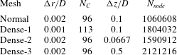
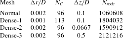
To quantify the effect of mesh density on the numerical results, simulations using three additional meshes of different densities are performed at
 $\unicode[STIX]{x1D6FC}=6$
and
 $Re=500$
, i.e. the maximum rotation rate and the largest Reynolds number in the present study. The properties of these meshes are listed in table 1, where
 $\unicode[STIX]{x0394}r$
,
 $Nc$
,
 $\unicode[STIX]{x0394}z$
and
 $N_{node}$
stand for the radial mesh size on the cylinder surface, the number of elements along the circumference of the cylinder surface, the mesh size along the cylinder span and the total number of nodes of the mesh, respectively. The normal and dense-1 mesh have the same number of elements along the spanwise direction of the cylinder but different mesh densities on the
 $x-y$
-plane. The layers of the elements in the spanwise direction of the dense-2 and dense-3 meshes are higher than those of the normal mesh. The time histories of the lift coefficient of the cylinder calculated from the four different meshes are compared with each other in figure 1(c). The lift and drag coefficients are defined as
 $C_{L}=F_{L}/(\unicode[STIX]{x1D70C}DLU^{2}/2)$
and
 $C_{D}=F_{D}/(\unicode[STIX]{x1D70C}DLU^{2}/2)$
, where
 $F_{L}$
and
 $F_{D}$
are the total lift and drag forces on the whole cylinder, respectively. The lift coefficient is found to oscillate with time very irregularly, similar to what is observed for the lift coefficient at
 $Re=200$
and
 $\unicode[STIX]{x1D6FC}=4.5$
reported by Navrose et al. (Reference Meena and Mittal2015). Initially, the lift coefficients from all the meshes follow a similar trend and are nearly the same until approximately
 $t=10$
, after which they start to oscillate. Because the lift coefficient oscillation is very irregular, the curves in figure 1(c) are not repeatable and as a result, the lift coefficients from different meshes are sometime out of phase with each other and sometimes in phase with each other. Therefore, there are points in the time histories where the maximum and the minimum lift coefficients from different meshes become very close to each other when they are in phase.
Meshes used in the mesh dependency study for
 $\unicode[STIX]{x1D6FC}=6$
and
 $Re=500$
.
3 Results and discussion
Three-dimensional numerical simulations are performed for
 $Re=100$
, 150, 200, 250 and 500. For each Reynolds number, the rotation rate varies from 1.6 to 6 with an increment of 0.2. In the first part of this section, a detailed analysis of the flow structure for
 $Re=200$
is presented because all the identified flow regimes are found at
 $Re=200$
. Later, the formation dynamics of flow structures at different flow regimes for
 $Re=200$
is studied in detail. In the second part of this section, the transition of flow structures as a function of rotation rate for
 $Re=100$
, 150, 250 and 500 is discussed. In the last part of this section, lift and drag coefficients as a function of rotation rate are presented for different Reynolds numbers and comparison is made with the previous results.
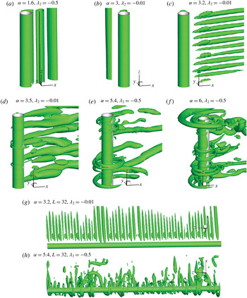
Vortex shedding patterns at
 $Re=200$
represented by iso-surfaces of the second eigenvalue
 $\unicode[STIX]{x1D706}_{2}$
.

3.1 Case
 $Re=$
200

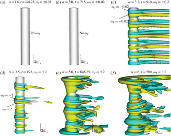
Iso-surfaces of tangential vorticity
 $\unicode[STIX]{x1D714}_{T}$
for
 $Re=200$
.

It is well known that
 $Re=200$
is the critical Reynolds number where the flow in the wake of a non-rotating cylinder transitions from two-dimensional to three-dimensional in numerical simulations (Zhao et al.
Reference Zhao, Thapa, Cheng and Zhou2013). The results for
 $Re=200$
are presented first because all the flow patterns around the cylinder found for other Reynolds numbers are observed for
 $Re=200$
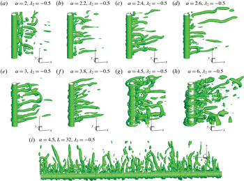
. Figure 2 shows the selected two- and three-dimensional vortex flow patterns near the cylinder for
 $Re=200$
and a number of rotation rates from
 $\unicode[STIX]{x1D6FC}=1.6$
to 6. The vortex shedding patterns are presented by the eigenvalue
 $\unicode[STIX]{x1D706}_{2}$
of the tensor defined as
 $\unicode[STIX]{x1D63F}^{2}+\unicode[STIX]{x1D734}^{2}$
, where
 $\unicode[STIX]{x1D63F}$
and
 $\unicode[STIX]{x1D734}$
are the symmetric and anti-symmetric parts of the velocity-gradient tensor, respectively. The topology and geometry of vortex cores for various flow conditions can be correctly presented using
 $\unicode[STIX]{x1D706}_{2}$
(Jeong & Hussain Reference Jeong and Hussain1995). It can be seen from figure 2 that circular vortices wrapped around the cylinder surface are observed at large rotation rates (
 $\unicode[STIX]{x1D6FC}\geqslant 3.5$
). These circular vortices are referred to as ring-shaped vortices in this study. In order to have a better visualization of the ring-shaped vortices, the iso-surfaces of the vorticity in the tangential direction of the cylinder surface (referred to as the tangent vorticity hereafter) are presented in figure 3. The tangent vorticity is defined as
 $\unicode[STIX]{x1D714}_{T}=\unicode[STIX]{x1D714}_{x}\sin \unicode[STIX]{x1D703}-\unicode[STIX]{x1D714}_{y}\cos \unicode[STIX]{x1D703}$
, where
 $\unicode[STIX]{x1D714}_{x}$
,
 $\unicode[STIX]{x1D714}_{y}$
and
 $\unicode[STIX]{x1D714}_{z}$
are the non-dimensional vorticity in the
 $x$
-,
 $y$
- and
 $z$
-directions, respectively, and
 $\unicode[STIX]{x1D703}$
is the angular position of a point on the
 $x$
–
 $y$
plane. Using the Landau oscillator model, El Akoury et al. (Reference El Akoury, Braza, Perrin, Harran and Hoara2008) reported that the rotation of the cylinder delays the transition of the wake flow to three-dimensional flow from
 $Re=200$
to
 $Re=219.8$
when
 $\unicode[STIX]{x1D6FC}=0.5$
. Rao et al. (Reference Rao, Leontini, Thompson and Hourigan2013a
,Reference Rao, Leontini, Thompson and Hourigan
b
) and Navrose et al. (Reference Meena and Mittal2015) performed linear stability analyses at
 $Re\leqslant 400$
and a wide range of rotation rates (
 $\unicode[STIX]{x1D6FC}\leqslant 5$
) to study the flow transition from two- to three-dimensional flow. They identified different three-dimensional modes of instability associated with both unsteady flow (
 $\unicode[STIX]{x1D6FC}\leqslant 2$
) and steady flow (
 $\unicode[STIX]{x1D6FC}>2$
) at higher rotation rate. The effects of the rotation rate on the three-dimensionality of the wake flow can be clearly seen in figure 2. The flow at
 $\unicode[STIX]{x1D6FC}=1.6$
is two-dimensional and vortices are periodically shed from both sides of the cylinder. This mode of periodic vortex shedding is defined as the 2-D vortex shedding (VS-2D) mode also referred to as 2-D mode I vortex shedding. The VS-2D mode is similar to the wake flow around a non-rotating cylinder but is asymmetric. As the rotation rate is increased beyond a critical value, the vortex shedding is suppressed, and the flow becomes steady. This type of flow is referred to as a 2-D steady state (SS-2D) mode in this study and the critical rotation rate for the flow transition from the VS-2D to the SS-2D mode for
 $Re=200$
is
 $\unicode[STIX]{x1D6FC}=2.1$
. The VS-2D and SS-2D modes are the same as the ones reported in previous 2-D numerical studies (Lu et al.
Reference Lu, Qin, Teng and Li2011). The wake flow at
 $Re=200$
remains in the SS-2D mode without vortex shedding in the range of rotation rates of
 $2.2\leqslant \unicode[STIX]{x1D6FC}\leqslant 3$
. Navrose et al. (Reference Meena and Mittal2015) also found the steady state mode in this range of rotation rates in their DNS study conducted at
 $Re=200$
.
Zhao et al. (Reference Zhao, Thapa, Cheng and Zhou2013) simulated flow past a non-rotating cylinder using the same numerical model and found that the flow at
 $Re=200$
is two-dimensional. It is interesting to observe that the rotation rate also delays the transition of the wake flow from two- to three-dimensional in the VS-2D and SS-2D modes. However, as the rotation rate is increased to
 $\unicode[STIX]{x1D6FC}=3.2$
(see figure 2
c), the flow for
 $Re=200$
becomes weekly three-dimensional with the occurrence of so-called finger-type vortices, where the elongated streamwise vortices are generated from one side of the cylinder and dominate the wake flow. These finger-shaped vortices (FVs) are distributed along the spanwise direction of the cylinder and are almost equidistant from each other. The vortices are so weak in figure 2(c) that they can only be identified using iso-surfaces of the very small eigenvalue of
 $\unicode[STIX]{x1D706}_{2}=-0.01$
. The vortex flow mode in figure 2(c) is referred to as a finger-shaped vortex mode. The so-called finger-shaped vortex mode was also found using the linear stability analysis performed by Navrose et al. (Reference Meena and Mittal2015) and they referred to it as a Mode E instability. It was found that FV mode is the first unstable three-dimensional mode as the rotation rate is increased beyond the boundary of the rotation rate range for steady state flow. The lower boundary of rotation rate for Mode E at
 $Re=200$
was found to be
 $\unicode[STIX]{x1D6FC}=3.01$
in Navrose et al. (Reference Meena and Mittal2015), which is the same as the lower boundary of the FV mode in this study.
As
 $\unicode[STIX]{x1D6FC}$
is increased to 3.5, ring-shaped vortices (RVs) are generated and they wrap around the cylinder surface, as shown in figure 2(d). However, the RVs are still weaker than the FVs and the distribution of FVs along the cylinder span becomes irregular. With an increase in the rotation rate, the strength of the RVs increases and the FVs gradually become secondary. This is evident at
 $\unicode[STIX]{x1D6FC}=5.4$
and 6 where large RVs wrapped around the surface of the cylinder at different locations are clearly visible by the iso-surfaces of
 $\unicode[STIX]{x1D706}_{2}=-0.5$
and no well-defined FVs exist. The vortex flow pattern with RVs is defined as the RV mode in this study, regardless of whether the RVs are stronger or weaker than the FVs. Mittal (Reference Mittal2004) in his DNS study at
 $Re=200$
and
 $\unicode[STIX]{x1D6FC}\leqslant 5$
attributed the RVs to the centrifugal instabilities present along the entire span of the cylinder. However, he did not classify them in his study nor did he attempt to explain the physics of the associated flow structures.
To ensure that the cylinder length of
 $L=6.4$
is sufficient to predict the three-dimensional flow structures, two additional simulations with a cylinder length of
 $L=32$
and
 $\unicode[STIX]{x1D6FC}=3.2$
and 5.4 are conducted and the predicted flow structures are shown in figures 2(g) and 2(h), respectively. The FV mode and the RV mode simulated using
 $L=32$
are the same as their counterparts obtained using
 $L=6.4$
. There are 54 FVs along the
 $L=32$
cylinder span in figure 2(g), corresponding to a spacing of approximately 0.59, which is nearly the same as the FV spacing in figure 2(c) corresponding to
 $L=6.4$
. For
 $\unicode[STIX]{x1D6FC}=5.4$
, the spacing between the RVs varies along the cylinder span, however, the maximum RV spacing in figure 2(h) is less than 6.4.
Since the flow is two-dimensional for both the VS-2D and SS-2D modes, the tangent vorticity is zero in both cases (figure 3
a,b). By observing the iso-surfaces of
 $\unicode[STIX]{x1D714}_{T}$
for
 $Re=200$
and
 $\unicode[STIX]{x1D6FC}=3.2$
in figure 3(c), it is conclusive that the tangential vorticities around the cylinder, indicating the presence of RVs, already occurs in the FV mode. However, the RVs are much weaker than the FVs and are located very close to the surface of the cylinder, therefore they cannot be identified in figure 2(c). Further examination of the iso-surface of
 $\unicode[STIX]{x1D714}_{T}$
revealed that the RVs distributed along the cylinder span are always in pairs, except near the ends of the cylinder. These RVs elongate from one side of the cylinder to form pairs of FVs which are equidistant from each other. Five and a half pairs of FVs are observed over a span length of
 $6.4D$
which corresponds to a non-dimensional wavelength of approximately 1.1–1.2. This wavelength agrees very well with the value of approximately 1 reported by Navrose et al. (Reference Meena and Mittal2015).
As
 $\unicode[STIX]{x1D6FC}$
increases from 3.2 to 3.5, the RVs which wrap around the cylinder surface remain in the proximity of the cylinder surface but are not evenly distributed along the cylinder span. With further increase in the rotation rate beyond
 $\unicode[STIX]{x1D6FC}=4$
, the three-dimensionality of flow is different from that for smaller
 $\unicode[STIX]{x1D6FC}$
in the following ways. Firstly, the ring-shaped vortices become dominant over the finger-shaped vortices. Secondly, the distribution of the ring-shaped vortices along the spanwise direction of the cylinder becomes irregular. Thirdly, RVs are found to move away from the surface of the cylinder, forming bigger rings. It is also observed that the vorticity in the tangential direction has increased drastically. This change in the flow structure at
 $\unicode[STIX]{x1D6FC}\geqslant 4$
has previously been reported through linear stability analyses by Rao et al. (Reference Rao, Leontini, Thompson and Hourigan2013a
,Reference Rao, Leontini, Thompson and Hourigan
b
) and Navrose et al. (Reference Meena and Mittal2015), who found that the combination of mode E and mode H instabilities at
 $\unicode[STIX]{x1D6FC}\geqslant 4.5$
makes the flow irregular.
Based on the above discussion, the vortex flow modes identified for
 $Re=200$
are summarized below:
(i) VS-2D (
$\unicode[STIX]{x1D6FC}\leqslant 2$
): 2-D wake vortex shedding similar to the vortex shedding from a non-rotating cylinder.(ii) SS-2D (
$2.2\leqslant \unicode[STIX]{x1D6FC}\leqslant 3$
): wake flow is steady 2-D flow and there is no vortex shedding.(iii) FV (
$3.2\leqslant \unicode[STIX]{x1D6FC}\leqslant 3.4$
): wake flow is dominated by 3-D FVs with very weak RVs wrapping the cylinder surface.(iv) RV (
$3.5\leqslant \unicode[STIX]{x1D6FC}\leqslant 6$
): wake flow is characterized by the occurrence of RVs, whose strength increases with increasing
$\unicode[STIX]{x1D6FC}$
.


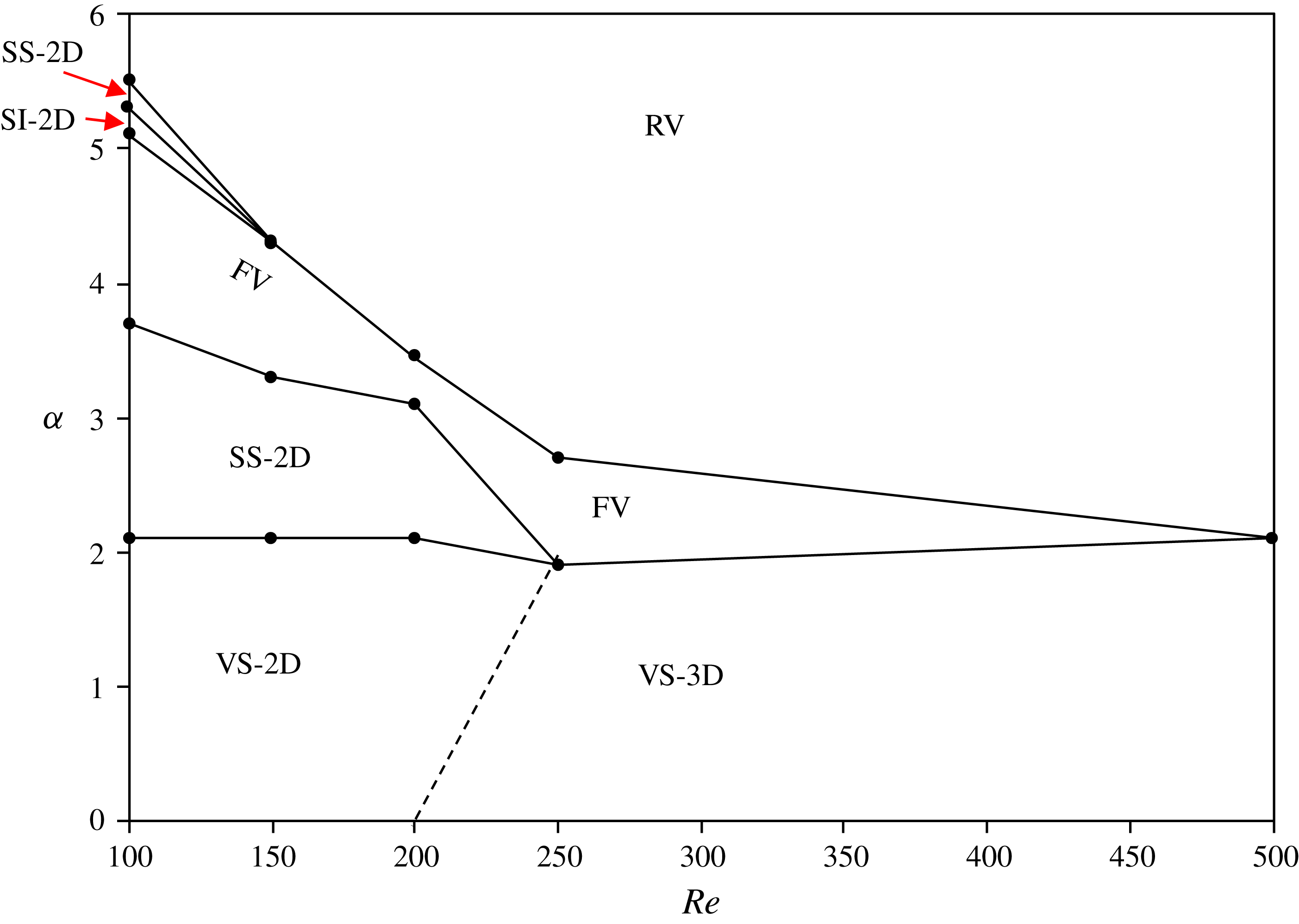
The identified flow regimes for all the simulated Reynolds numbers (
 $Re\leqslant 500$
) and
 $\unicode[STIX]{x1D6FC}$
are mapped on the
 $Re$
-
 $\unicode[STIX]{x1D6FC}$
space in figure 4. The flow is two-dimensional vortex shedding flow at
 $\unicode[STIX]{x1D6FC}\leqslant 2$
for
 $Re=100$
, 150 and 200 and
 $\unicode[STIX]{x1D6FC}\leqslant 1.8$
for
 $Re=250$
. If vortices are periodically shed from both sides of the cylinder and the flow is two-dimensional, the flow mode is referred to as the VS-2D mode. Although periodic vortex shedding takes place at
 $Re=500$
and
 $\unicode[STIX]{x1D6FC}\leqslant 2$
, the flow in the wake of the cylinder is three-dimensional and is referred to as VS-3D. As the rotation rate is increased further from
 $Re=100$
to 200, the flow transitions from the VS-2D mode to the SS-2D mode. The critical rotation rate for transition of the flow to the no vortex shedding regime in the previous 2-D numerical results by El Akoury et al. (Reference El Akoury, Braza, Perrin, Harran and Hoara2008) is found to be in good agreement with the ones obtained in the present study for
 $Re\leqslant 200$
. The SS mode is not observed for
 $Re\geqslant 250$
due to the three-dimensionality of the flow. It can be seen that with the Reynolds number decreasing, the range of
 $\unicode[STIX]{x1D6FC}$
for the SS-2D mode becomes broader and the FV mode occurs at higher rotation rates. As seen previously in figure 3, the three-dimensionality of the flow starts with the occurrence of FVs in the wake of the cylinder accompanied by very week RVs. The FVs become irregular with further increase in the rotation rate whereas the RVs increase in strength and begin to move away from the cylinder. The flow structures at large rotation rates are dominated by RVs and the critical rotation rate between the FV and the RV modes in figure 4 decreases with increasing Reynolds number. It is worth noting that FVs are not observed at
 $Re=500$
. At higher rotation rate, the flow becomes very irregular and chaotic with an irregular distribution of large RVs along the spanwise direction of the cylinder. An interesting phenomenon observed at
 $Re=100$
is the occurrence of a two-dimensional secondary instability (SI-2D) at
 $\unicode[STIX]{x1D6FC}=5.2$
and a secondary SS-2D mode at
 $\unicode[STIX]{x1D6FC}=5.4$
. The SI-2D mode is a typical flow mode that has previously been observed at
 $Re=100$
for a very small range of
 $\unicode[STIX]{x1D6FC}$
(Lu et al.
Reference Lu, Qin, Teng and Li2011). The flow at
 $Re=100$
transitions into a 3-D RV mode as
 $\unicode[STIX]{x1D6FC}$
exceeds 5.5 because the instability of the flow increases with increasing
 $\unicode[STIX]{x1D6FC}$
. This results in significant increase in the three-dimensionality of the flow. The secondary SS-2D mode and SI-2D mode are not found for
 $Re=150$
and above. The detailed motions of the vortices for different flow modes at
 $Re=200$
are discussed in detail in this section and the flow modes for all other Reynolds numbers will be discussed in § 3.2.
Map of the flow regimes on the
 $Re$
-
 $\unicode[STIX]{x1D6FC}$
space.

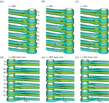
The dynamics of the FVs and RVs can be explained by figure 5 which shows the iso-surfaces of
 $\unicode[STIX]{x1D714}_{T}=\pm 0.2$
for the FV mode at
 $Re=200$
and
 $\unicode[STIX]{x1D6FC}=3.2$
. Five whole pairs of tangent vortices (labelled as A to E) are observed along the spanwise direction of the cylinder, excluding the single tangent vortex at the bottom end of the cylinder, as shown in figure 5. The tangent vortices elongate in the wake of the cylinder forming FVs mainly from one side of the cylinder. As a result, five pairs of FVs exist in the wake of the cylinder. At
 $t=900$
, figure 5(d) shows that the two vortices are close to each other within each of pairs A, B, C and E and separated from each other in pair D. The two vortices in a pair slide periodically towards and away from each other along the surface of the cylinder, which can be clearly seen in figure 5(d–f). For example, the two vortices in vortex pair D, which are very separated from each other at
 $t=900$
, become close to each other at
 $t=905$
and separated from each other again at
 $t=910$
. The repetitive separation and closeness between two vortices occur within every vortex pair and are found to be periodic. Every time after the distance between two RVs in a pair reaches its maximum, the two RVs start to move towards each other and vice versa. It is also observed that whenever the two RVs in a pair are close to each other, their corresponding FVs shrink in size, and whenever they separate from each other the FVs grow in size. The single vortex at the bottom end of the cylinder does not change its position and remains isolated all the time.
Three-dimensional vortex shedding patterns of iso-surface of tangential component of vorticity
 $\unicode[STIX]{x1D714}_{T}=\pm 0.2$
at
 $Re=200$
and
 $\unicode[STIX]{x1D6FC}=3.2$
.

When
 $Re=200$
and
 $\unicode[STIX]{x1D6FC}=3.2$
, the ring-shaped vortices develop near the cylinder surface. However, they are found to be too weak to be seen in the flow field. To illustrate the correlation between the RV distribution along the cylinder span and the pressure on the cylinder surface, the perturbation velocity and pressure are defined as
 $(u^{\prime },v^{\prime },w^{\prime },p^{\prime })=(u,v,w,p)-(\overline{u},\overline{v},\overline{w},\overline{p})$
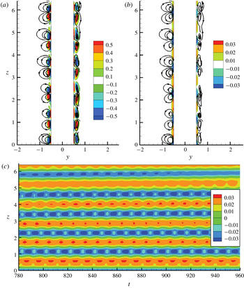
, where the prime stands for the perturbation part and the overbar stands for temporal-spatial averaged value over time and cylinder span. Figure 6(a) shows the streamlines based on the perturbed velocity and the contours of the perturbation tangent vorticity
 $\unicode[STIX]{x1D714}_{T}^{\prime }$
on the
 $y$
–
 $z$
plane; figure 6(b) shows the contours of
 $p^{\prime }$
and streamlines; and figure 6(c) shows the temporal and spatial evolution of
 $p^{\prime }$
along the line of
 $x=0$
and
 $y=0.51$
near the surface of the cylinder for
 $Re=200$
and
 $\unicode[STIX]{x1D6FC}=3.2$
.
(a) Streamlines contours of
 $\unicode[STIX]{x1D714}_{T}^{\prime }$
based on the perturbation velocity on the
 $y$
–
 $z$
plane at
 $t=905$
; (b) streamlines based on the perturbation velocity and contours of pressure
 $p^{\prime }$
on the
 $y$
–
 $z$
plane at
 $t=905$
; (c) temporal and spatial evolution of
 $p^{\prime }$
along the line
 $x=0$
,
 $y=0.51D$
for
 $Re=200$
and
 $\unicode[STIX]{x1D6FC}=3.2$
.

Five and a half vortex pairs can be clearly identified in figure 6(a) and they are almost evenly distributed along the cylinder span. There are shear layers between the vortex pairs and the cylinder surface. The wavelength of the undulation of the pressure distribution along the cylinder span is the same as the distance between two neighbouring vortex pairs in figure 6(b). Immediately above the cylinder surface, the perturbation velocity follows the perturbation pressure gradient in the
 $z$
-direction. The convergence of the streamline in the low pressure zone makes the shear layers roll up, forming two recirculation zones in opposite directions. As a result, the centre of each vortex pair is a low
 $p^{\prime }$
zone where streamlines converge (see figure 6
b).
The centres of the five RV pairs A–E in figure 6 can easily be correlated to the low pressure stripes in figure 6(c). The spatial distribution of vortex pairs along the cylinder makes the pressure fluctuate periodically along the spanwise direction of the cylinder. The periodic separation and closeness of the two RVs in each vortex pair makes the pressure also vary periodically with time. Whenever the two RVs in a vortex pair become close to each other, the pressure on the cylinder surface between them decreases and vice versa. Based on the periodic variation of the pressure with time in figure 6(c), it can be concluded that the motion of the RVs along the spanwise direction of the cylinder is periodic. It is also found based on figure 6(c) that the variations of the pressure in stripes A and D are out of phase with those of the rest of the pressure stripes, indicating that the motion of all the vortex pairs are not synchronized. It is further observed that the stripes in figure 6(c) remain almost straight and do not vary significantly along the
 $t$
–
 $z$
plane, indicating that the vortices oscillate about fixed mean positions.
Each low pressure stripe in figure 6(c) along the
 $t$
–
 $z$
plane corresponds to a streamline contraction point in figure 6(a) located at the centre of the two RVs in a pair, and each high pressure stripe corresponds to the centre of the two adjacent RV pairs, which is a stagnation point in figure 6(a).
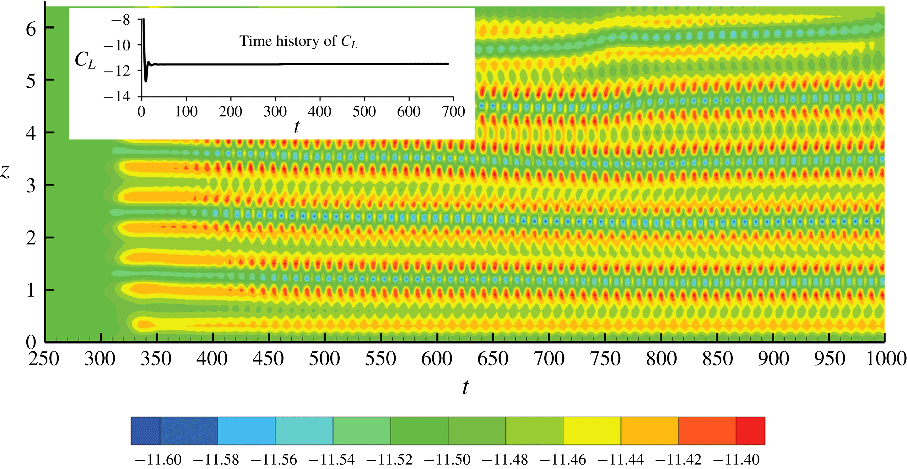
Contours of the oscillatory sectional lift coefficient on the
 $t$
–
 $z$
plane for
 $Re=200$
and
 $\unicode[STIX]{x1D6FC}=3.2$
.

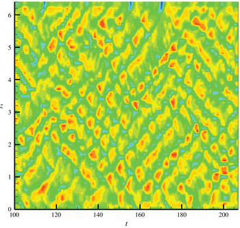
Figure 7 shows the contours of the sectional lift coefficient on the
 $t$
–
 $z$
plane for
 $Re=200$
and
 $\unicode[STIX]{x1D6FC}=3.2$
. The sectional lift coefficient at a location of
 $z$
is defined as
 $C_{L}(z)=F_{L}(z)/(\unicode[STIX]{x1D70C}DU^{2}/2)$
, where the sectional lift force
 $F_{L}(z)$
is calculated by integrating the pressure and shear stress over the circumference of the cylinder at
 $z$
. The mean value of all the sectional lift coefficients on the cylinder span is negative because the rotation of the cylinder causes asymmetric flow. However, the sectional lift coefficient, which was nearly constant before
 $t=300$
, starts to oscillate about negative mean values at
 $t>300$
, indicating that the flow transition to three-dimensional starts at
 $t\approx 300$
. The oscillation of the pressure on the cylinder caused by the oscillatory motion of the vortices along the cylinder span is responsible for the oscillation of the sectional lift coefficient. The frequencies of the oscillation of the sectional lift coefficient in figure 7 and the oscillation of the pressure coefficient in figure 6 are the same. The time history of the lift coefficient on the entire cylinder (referred to as the lift coefficient hereafter) is shown on top of the sectional lift coefficient contours in figure 7. Since the oscillations of the sectional lift coefficient along the entire span of the cylinder have random phases (sometimes in phase and sometime out of phase with each other), the lift coefficient on the whole cylinder is nearly constant and does not oscillate.
Three-dimensional vortex shedding patterns of iso-surface of tangential component of vorticity
 $\unicode[STIX]{x1D714}_{T}=\pm 1$
at
 $Re=200$
and
 $\unicode[STIX]{x1D6FC}=3.5$
.

Although the two vortices in each vortex pair may become close to or far from each other periodically, the mean position of the vortex pair does not change at
 $Re=200$
and
 $\unicode[STIX]{x1D6FC}=3.2$
since the vortex pair always oscillates about its fixed mean position. As the rotation rate is increased to
 $\unicode[STIX]{x1D6FC}=3.5$
and the Reynolds number remains fixed at
 $Re=200$
, the RVs become much more dynamic and are distributed irregularly on the cylinder span. When
 $\unicode[STIX]{x1D6FC}$
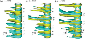
is increased from 3.2 to 3.5, the tangent vortices become strong enough to be identified using the total velocity, instead of the perturbation velocity. Figure 8 shows the iso-surfaces of
 $\unicode[STIX]{x1D714}_{T}\pm 1$
for
 $Re=200$
and
 $\unicode[STIX]{x1D6FC}=3.5$
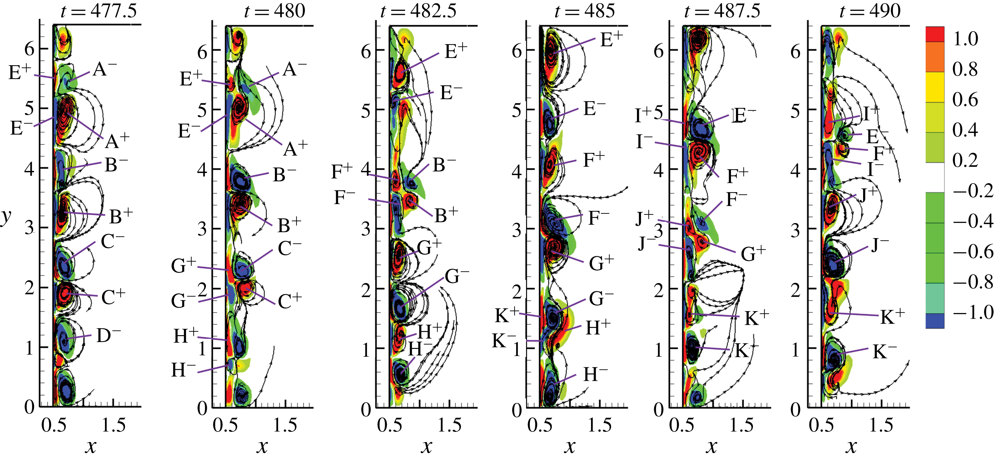
, figure 9 shows the contours of the tangent vorticity
 $\unicode[STIX]{x1D714}_{T}$
on the
 $y$
–
 $z$
plane and figure 10 shows the evolution of the pressure coefficient along the vertical line of
 $x=0$
and
 $y=0.51$
for the same case. The vortex pairs on the cylinder labelled A to D in figure 8 are not distributed evenly along the cylinder span. In figure 8(a), the two RVs in pair B have the largest gap between them. In addition to the vortex pairs, two single vortices are also present at the two ends of the cylinder, respectively. The four pairs of RVs correspond to the four pairs of vortices on the
 $y$
–
 $z$
plane in figure 9. Compared with those for
 $\unicode[STIX]{x1D6FC}=3.2$
, the vortex pairs in figure 9 are found to move away from the cylinder surface in the radial direction. For instance, the two RVs in pair B in figure 9 grows as
 $t$
increases from 477.5 to 480. The new pair F develops under pair B, pushes pair B outside the cylinder surface at
 $t=482.5$
and becomes the dominant vortex pair at
 $t=485$
. Similarly, the growth of vortex pairs E and G makes vortex pairs A and C move outwards and dissipate, respectively. Another interesting phenomenon of the vortex motion at
 $\unicode[STIX]{x1D6FC}=3.5$
is the regrouping of the vortices. Taking the time from
 $t=482.5$
to 485 as an example, one RV from pair F and one RV from pair G regroup together, forming a new pair. At
 $t=482.5$
, the RV with positive
 $\unicode[STIX]{x1D714}_{T}$
is on top and the RV with the negative
 $\unicode[STIX]{x1D714}_{T}$
is on the bottom in each of pairs F and G. After the dissipation of the outer layer vortices and regrouping of the newly grown vortices, the RV with positive
 $\unicode[STIX]{x1D714}_{T}$
is at the top side of each pair at
 $t=485$
for pairs F
 $^{-}$
G
 $^{+}$
and E
 $^{-}$
F
 $^{+}$
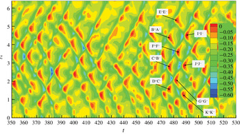
. The regrouping of the vortex pairs only occurs at the second layer of the vortices from the cylinder surface. The generation of new RVs, dissipation of the old RVs and regrouping of the vortex pairs happens continuously and periodically. This can be proven by the pressure distribution on the
 $t$
–
 $z$
plane in figure 10.
Contours of the tangent vorticity
 $\unicode[STIX]{x1D714}_{T}$
on the
 $y$
–
 $z$
plane for
 $Re=200$
and
 $\unicode[STIX]{x1D6FC}=3.5$
. The superscripts ‘
 $+$
’ and ‘
 $-$
’ stand for positive and negative tangent vortices, respectively.

The pressure coefficient distribution for
 $\unicode[STIX]{x1D6FC}=3.5$
and
 $Re=200$
in figure 10 is in a staggered arrangement like fish scales, instead of stripes as that for
 $\unicode[STIX]{x1D6FC}=3.2$
and the same
 $Re=200$
. The staggered distribution of positive and negative streamwise vortices on the cylinder span is due to the movement of the vortices in the radial direction, as shown in figure 9. This results in the undulation of the pressure along the
 $z$
-direction in figure 10. The maximum pressures are in a staggered arrangement in time because of the continuous regeneration of new RVs from the cylinder surface. It is found in figure 6(a) that a maximum or minimum pressure on the cylinder surface occurs at the boundaries between two vortices. On the
 $y$
–
 $z$
plane, a maximum pressure occurs between two vortex pairs with one negative vortex on the top and one positive vortex on the bottom, while a minimum pressure occurs between two vortex pairs with one positive vortex on the top and one negative vortex on the bottom. The local high pressures caused by vortex pairs E
 $^{+}$
E
 $^{-}$
, B
 $^{+}$
A
 $^{-}$
, etc. are marked on the pressure contours in figure 10. For example, at
 $t=477.5$
the two vortices, C
 $^{-}$
on the top and C
 $^{+}$
on the bottom, create a minimum pressure at approximately
 $y=2.1$
; G
 $^{-}$
and G
 $^{+}$
grow between
 $t=477.5$
and 482.5 and replace C
 $^{-}$
and C
 $^{+}$
. Because every newly generated vortex on the bottom layer has an opposite direction to that of the vortex on top of it, C
 $^{-}$
on the top and C
 $^{+}$
on the bottom at
 $t=477.5$
are followed by G
 $^{+}$
on the top and G
 $^{-}$
on the bottom at
 $t=482.5$
. Correspondingly, the minimum pressure at approximately
 $y=2.1$
will be followed by a maximum pressure at the same location. This alternative occurrence of minimum and minimum pressures at a fixed location results in the fish-scale-shaped pressure distribution in figure 10.
Temporal and spatial evolution of the pressure along the line
 $x=0$
,
 $y=0.51$
at
 $Re=200$
and
 $\unicode[STIX]{x1D6FC}=3.5$
. The marked maximum pressures created by the vortices indicated in figure 9.

Compared with that for
 $\unicode[STIX]{x1D6FC}=3.2$
, the strength of RVs for
 $\unicode[STIX]{x1D6FC}=3.5$
is much stronger. The RVs for
 $\unicode[STIX]{x1D6FC}=3.2$
are too weak to be seen from the iso-surfaces of
 $\unicode[STIX]{x1D706}_{2}$
in figure 2(c) because they are overwhelmed by the streamwise FVs. The increase in the strength of the RVs at
 $\unicode[STIX]{x1D6FC}=3.5$
make RVs visible from the iso-surface of
 $\unicode[STIX]{x1D706}_{2}$
in figure 2(d). In the RV mode, the RVs are repetitively generated from the surface of the cylinder, grow in size, move outwards in the radial direction and finally dissipate as they move far away from the cylinder. At
 $Re=200$
and
 $\unicode[STIX]{x1D6FC}=3.5$
, the generation and dissipation of RVs at a particular location on the cylinder span are generally periodic as depicted by the pressure variation in figure 10.
Iso-surfaces of
 $\unicode[STIX]{x1D706}_{2}=-1$
and the contours of the tangent vorticity
 $\unicode[STIX]{x1D714}_{T}$
for
 $Re=200$
and
 $\unicode[STIX]{x1D6FC}=6$
.

The strength and outward motion of the RVs in the radial direction observed for
 $Re=200$
and
 $\unicode[STIX]{x1D6FC}=3.5$
are found to be enhanced with increasing
 $\unicode[STIX]{x1D6FC}$
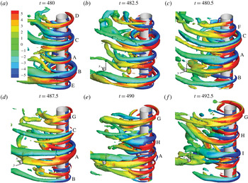
. Figure 11 shows the iso-surfaces of
 $\unicode[STIX]{x1D706}_{2}=-1$
together with the contours of the tangent vorticity
 $\unicode[STIX]{x1D714}_{T}$
for
 $Re=200$
and
 $\unicode[STIX]{x1D6FC}=6$
, where the motion of the RVs in the radial direction can be literally seen. The RVs are found to be in pairs generally except at the two ends of the cylinder. Every newly generated RV is a very small ring initially near the cylinder surface. It grows both in strength and diameter as times passes, and finally dissipates as it grows big enough. At
 $t=480$
, RV pair B and the single RV at the top end have fully grown in size whereas RV pair A has just started to evolve and RV pair C is growing in size. The outward motion of RV pairs A and C as they are growing can be clearly seen by observing their positions at figure 11(b,c). Although every RV pair dissipates at some stage, some RV pairs exist longer than others. For example, RV pair A, which started at
 $t=480$
and dissipates at
 $t=490$
, has a non-dimensional life span of approximately 10, while RV pair F only exists for an approximately non-dimensional time of 5, i.e. started at
 $t=480.25$
and disappeared at
 $t=487.5$
. The arrangement of the RV pairs at large
 $\unicode[STIX]{x1D6FC}$
is very irregular. The generation of new RV pairs usually occurs between two RV pairs with a large distance between them. An example is the generation of RV pair A between pairs B and C. This generation of RV pair A forces RV pair B to move towards the end of the cylinder where it is finally dissipated in the wake of the cylinder.
Iso-surfaces of
 $\unicode[STIX]{x1D706}_{2}$
for
 $Re=100$
and different
 $\unicode[STIX]{x1D6FC}$
.

3.2 Cases
$Re=$
100, 250 and 500

In this section, flow structures corresponding to
 $Re=100$
, 250 and 500 in the context of figure 4 are discussed and compared with the flow structure for
 $Re=200$
. The flow patterns identified in the previous section at
 $Re=200$
are also found for
 $Re=100$
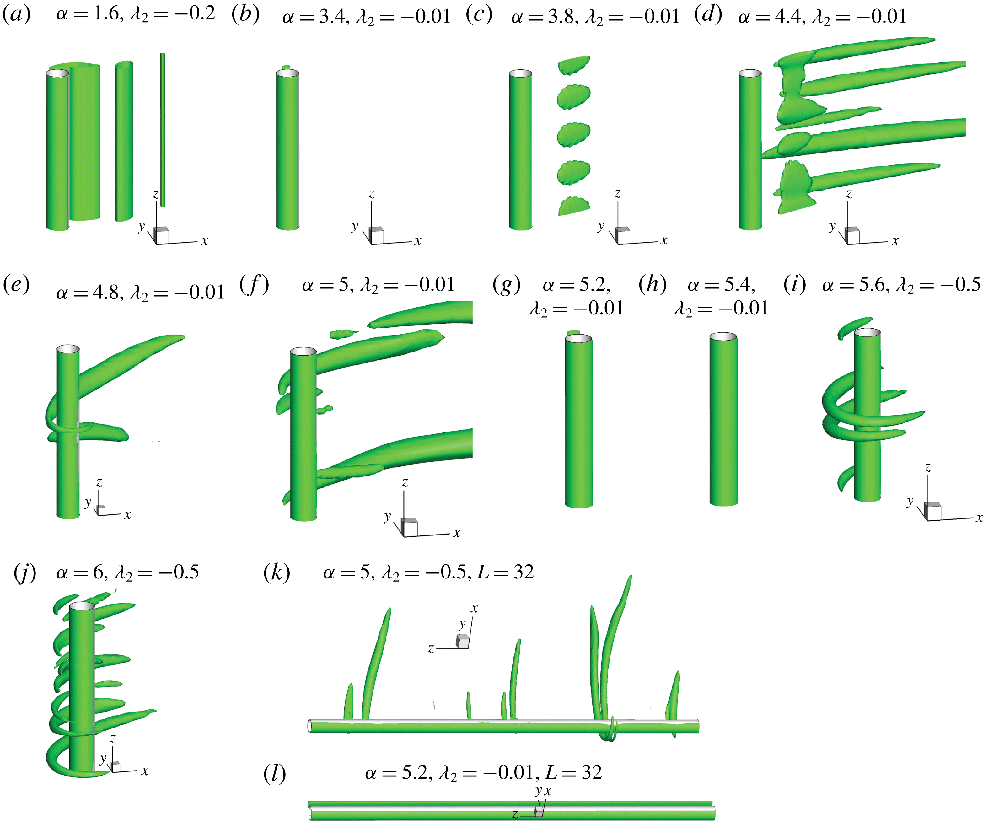
and the range of rotation rates as can be seen in figure 4. Figure 12 shows the vortex flow patterns for
 $Re=100$
at different
 $\unicode[STIX]{x1D6FC}$
represented by the eigenvalue
 $\unicode[STIX]{x1D706}_{2}$
. The flow pattern is in VS-2D mode for
 $\unicode[STIX]{x1D6FC}=1.6$
and SS-2D mode as
 $\unicode[STIX]{x1D6FC}=3.4$
(Mittal & Kumar Reference Mittal and Kumar2003; El Akoury et al.
Reference El Akoury, Braza, Perrin, Harran and Hoara2008). However, there are some differences in the flow structures in terms of the characteristics of the vortices at
 $Re=100$
compared to those at
 $Re=200$
at a higher rotation rate where the flow becomes three-dimensional. For example, the length and the number of the FVs at
 $Re=100$
and
 $\unicode[STIX]{x1D6FC}=3.8$
, which is the starting
 $\unicode[STIX]{x1D6FC}$
of three-dimensionality for
 $Re=100$
in figure 12(c), are much shorter and fewer in number as compared to
 $Re=200$
. The flow remains in the FV regime until
 $\unicode[STIX]{x1D6FC}=5$
. It is interesting to see that at
 $\unicode[STIX]{x1D6FC}=5.2$
and 5.4, the flow transitions into SI-2D and SS-2D modes, respectively, instead of changing to the RV mode, which starts from
 $\unicode[STIX]{x1D6FC}=5.6$
. To further demonstrate that the flow is intrinsically two-dimensional, simulations for a long cylinder with
 $L=32$
and
 $\unicode[STIX]{x1D6FC}=5.2$
and 5.4 are performed using the 3-D flow at
 $\unicode[STIX]{x1D6FC}=5$
as the initial conditions. The flow finally transitions from being initially three-dimensional to being two-dimensional, as shown in figure 12(l). When
 $\unicode[STIX]{x1D6FC}$
is near the lower boundary of the RV mode, the RVs are very sparsely distributed along the cylinder span, as shown in figure 12(i). At
 $\unicode[STIX]{x1D6FC}=5$
.6, there are only two pairs of RVs along the cylinder; one pair located at the centre and two isolated RVs at the two ends of the cylinder as shown in figure 12(i). When
 $\unicode[STIX]{x1D6FC}$
is increased to 6, there are multiple RVs along the cylinder in figure 12(j). The FVs near the top boundary of the FV regime are also very sparsely distributed along the cylinder as shown in figure 12(f), where
 $\unicode[STIX]{x1D6FC}=5$
. It is expected that the distance between FVs can be greater than the simulated length of the cylinder. To investigate the effect of length on the interval between two pairs of FVs and to have a better understanding of how FVs are distributed along a long cylinder span, a separate simulation of flow past a rotating cylinder with a non-dimensional length of 32,
 $Re=100$
and
 $\unicode[STIX]{x1D6FC}=5$
was conducted and the vortex flow structures are presented in figure 12(k). The FVs are found to be distributed sparsely without a constant spacing. The maximum non-dimensional gap between two FV pairs is greater than 6.4.
Another difference between the RVs at
 $Re=100$
in comparison to
 $Re=200$
is that the sizes of the RVs are much larger when
 $\unicode[STIX]{x1D6FC}$
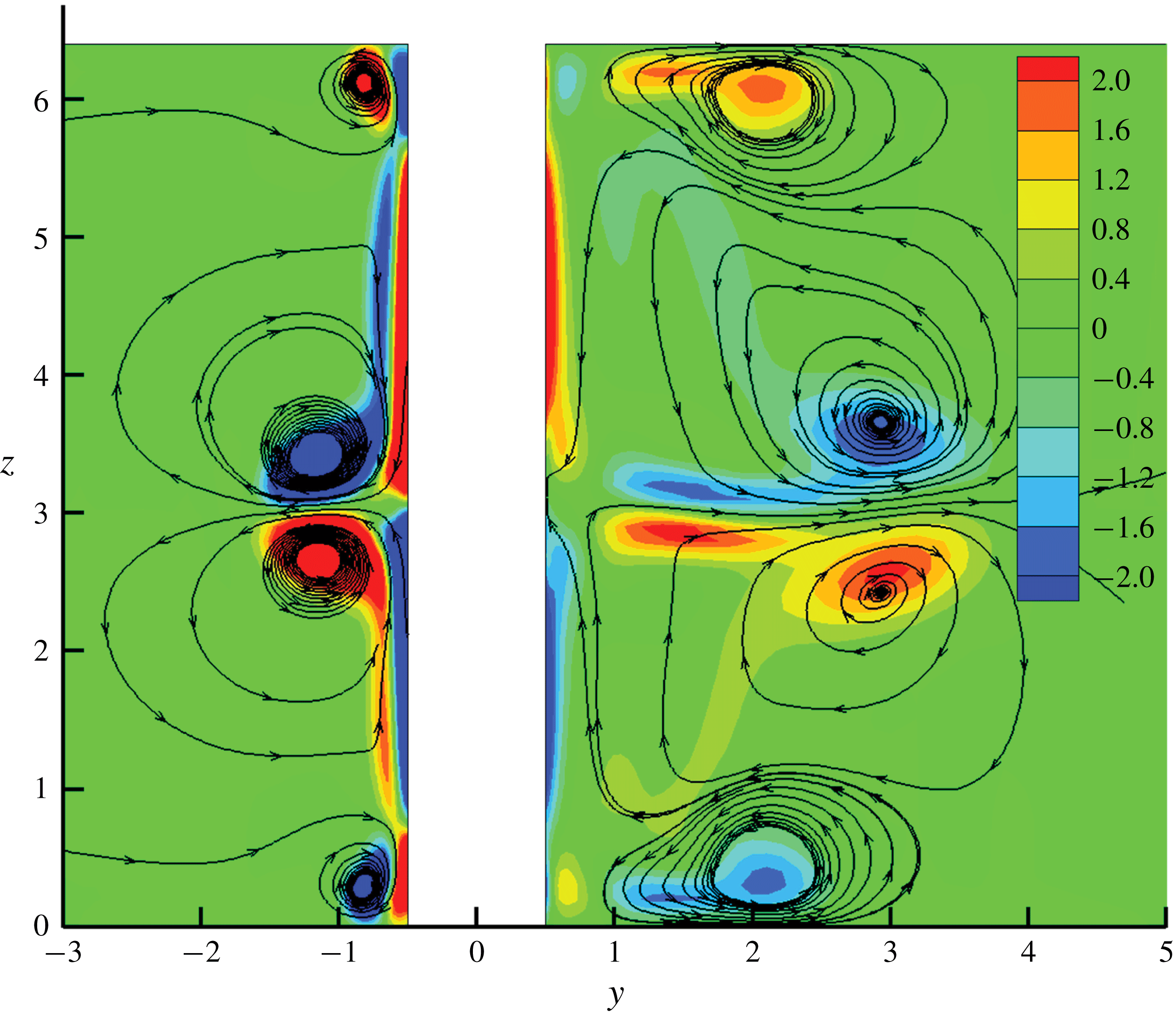
is small in the RV regime. Figure 13 shows the streamlines and contours of
 $\unicode[STIX]{x1D714}_{T}$
on the
 $y$
–
 $z$
plane for
 $Re=100$
and
 $\unicode[STIX]{x1D6FC}=5.6$
. The size of the RVs on the
 $y$
–
 $z$
plane for
 $Re=100$
is much greater than that for
 $Re=200$
. The large dimension of the RVs increases the distance between the centres of RVs and the cylinder surface which in turn increases the RV diameters. It is also the reason why the distances between the RVs for
 $Re=100$
are large. In figure 13, the RV pair occupy nearly the whole span of the cylinder. Although the size and number of the RVs are different, the formation mechanism and the characteristics of the RVs for
 $Re=100$
in the RV regime are the same as those for
 $Re=200$
.
Streamlines and contours of
 $\unicode[STIX]{x1D714}_{T}$
on the
 $y$
–
 $z$
plane for
 $Re=100$
and
 $\unicode[STIX]{x1D6FC}=5.6$
at
 $t=368.75$
.

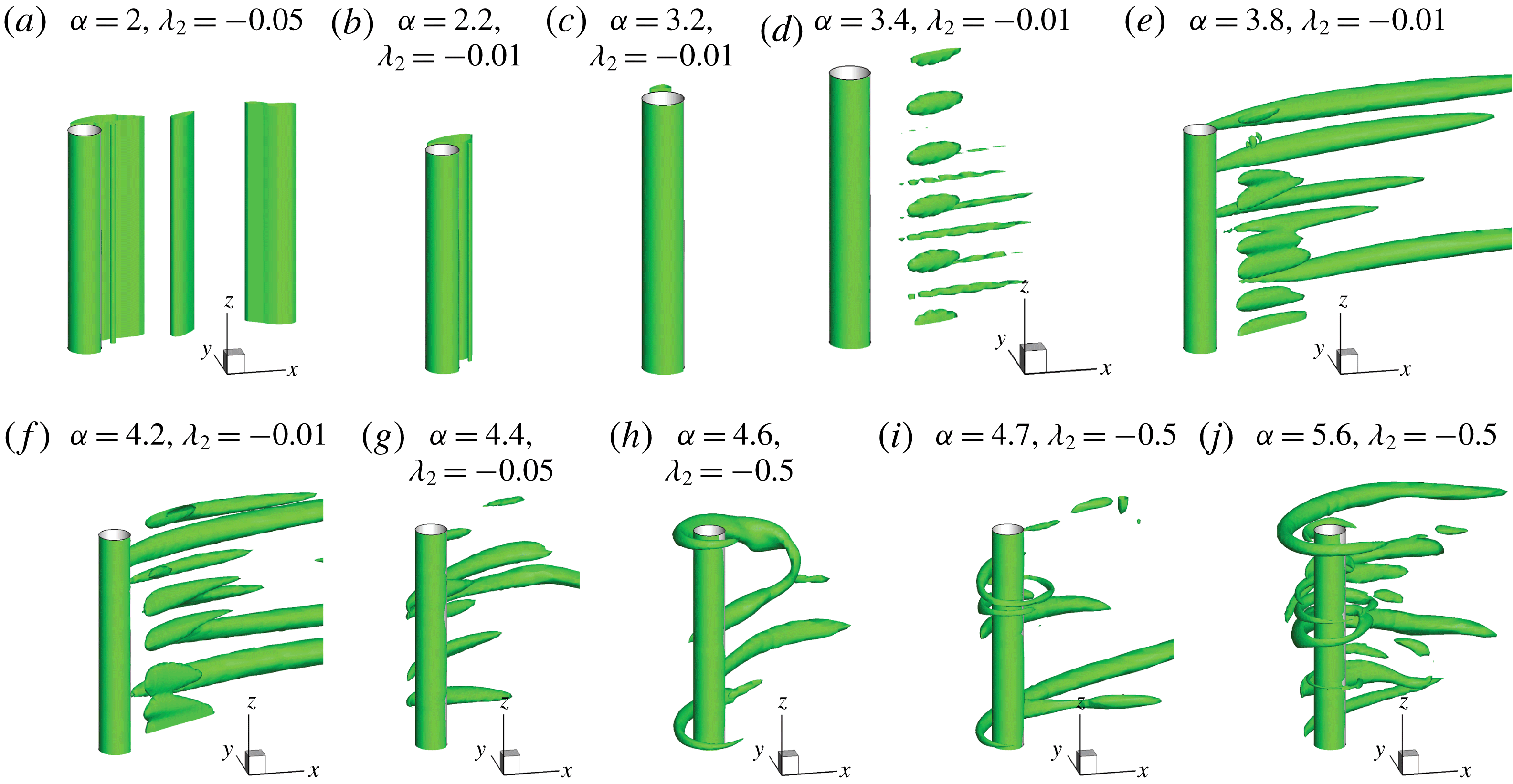
Figure 14 shows iso-surfaces of
 $\unicode[STIX]{x1D706}_{2}$
for
 $Re=150$
and different
 $\unicode[STIX]{x1D6FC}$
. From the vortex flow patterns, it can be concluded that the flow change from the VS-2D to the SS-2D mode as
 $\unicode[STIX]{x1D6FC}$
increases from 2 to 2.2; from the SS-2D to the FV mode as
 $\unicode[STIX]{x1D6FC}$
increases from 3.2 to 3.4; and from the FV to the RV mode as
 $\unicode[STIX]{x1D6FC}$
increases from 4.2 to 4.4. At
 $\unicode[STIX]{x1D6FC}=4.4$
, RVs elongate to form FVs in the wake of the cylinder which become much weaker than
 $\unicode[STIX]{x1D6FC}=4.2$
. Compared with
 $Re=100$
, the spacing between FVs in the FV mode is decreased. The secondary SS-2D mode between the FV and RV modes identified for
 $Re=100$
does not exist as
 $Re$
is increased to 150. Similar to that for
 $Re=100$
, the number of RVs along the cylinder span increases with the increase of
 $\unicode[STIX]{x1D6FC}$
.
Iso-surfaces of
 $\unicode[STIX]{x1D706}_{2}$
for
 $Re=150$
and different
 $\unicode[STIX]{x1D6FC}$
.

Iso-surfaces of
 $\unicode[STIX]{x1D706}_{2}$
for
 $Re=250$
and different
 $\unicode[STIX]{x1D6FC}$
.

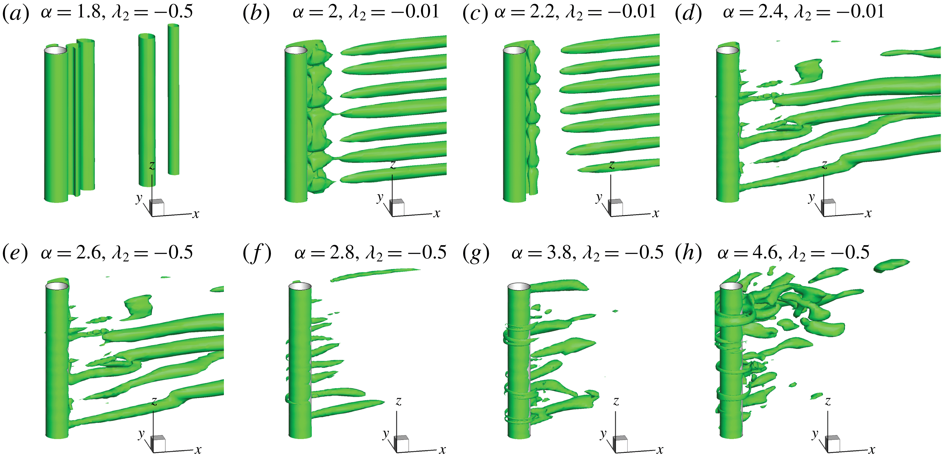
Figure 15 shows the iso-surfaces of
 $\unicode[STIX]{x1D706}_{2}$
for
 $Re=250$
and different
 $\unicode[STIX]{x1D6FC}$
. It can be seen from figure 15(a,b) that as
 $\unicode[STIX]{x1D6FC}$
is increased from 1.8 to 2, the flow transitions from the VS-2D mode to the FV mode directly and the SS-2D mode that has been observed at
 $Re=200$
is skipped. The FVs in the FV mode occur in the rotation rate range of
 $2.2\leqslant \unicode[STIX]{x1D6FC}\leqslant 2.6$
and are found to be irregularly arranged along the cylinder spanwise direction at large rotation rates, but still present as streamwise vortices. As
 $\unicode[STIX]{x1D6FC}$
is increased to 2.8, RVs are observed around the surface of the cylinder and, similar to those for
 $Re=200$
, their strength increases with increasing
 $\unicode[STIX]{x1D6FC}$
. It can clearly be observed by comparing figures 2 and 15 that the flow becomes more chaotic as the Reynolds number is increased to
 $Re=250$
in the same range of rotation rates. It is well known that flow transitions to three-dimensional as
 $Re$
exceeds 200 (Brede et al.
Reference Brede, Eckelmann and Rockwell1996). It is interesting to see that the rotation rate has a profound effect inside the VS-2D mode at
 $Re=250$
resulting in delayed transition to three-dimensional flow.
Figure 16 shows the iso-surfaces of
 $\unicode[STIX]{x1D706}_{2}$
for
 $Re=500$
and different
 $\unicode[STIX]{x1D6FC}$
. For
 $Re=500$
, vortex shedding flow in the range of
 $\unicode[STIX]{x1D6FC}\leqslant 2$
is three-dimensional and the flow mode is defined as VS-3D. The traditional vortex shedding disappears at
 $\unicode[STIX]{x1D6FC}\geqslant 2.2$
, where RVs occur along the span of the cylinder. It can be seen in figure 16(b) that very weak RVs begin to form around the cylinder along with some streamwise vortices in the wake at
 $\unicode[STIX]{x1D6FC}=2.2$
. However, wake vortices are not predominately aligned in the
 $x$
-direction as in the FV mode. The flow at
 $\unicode[STIX]{x1D6FC}=2.2$
is deemed to be in the RV mode because of the occurrence of RVs. At
 $Re=500$
, the flow changes from the VS-3D mode to the RV mode directly and the FV mode is skipped. It is further found that the strength and the diameter of the RVs increase with the increase in the rotation rate. An additional simulation for
 $Re=500$
and
 $\unicode[STIX]{x1D6FC}=4.5$
with a cylinder length of 32 was conducted and the flow structure for
 $L=32$
shown in figure 16(i) is the same as the one for
 $L=6.4$
in figure 16(g). The cylinder length of
 $L=6.4$
is sufficient to predict the three-dimensional flow structures for
 $Re=500$
since the spacing between RVs is far smaller than 6.4.
Iso-surfaces of
 $\unicode[STIX]{x1D706}_{2}$
for
 $Re=500$
and different
 $\unicode[STIX]{x1D6FC}$
.

Figure 17 shows the evolution of the pressure coefficient along the line of
 $y=0.51$
and
 $x=0$
for
 $Re=500$
and
 $\unicode[STIX]{x1D6FC}=3.2$
. The fish-scale-like, staggered pressure distribution in figure 16 is similar to that shown in figure 10 for
 $Re=200$
, indicating that the vortex dynamics near the cylinder in the RV mode for
 $Re=500$
and 200 are similar to each other. At a specific moment, the wavenumber of the pressure distribution along the cylinder span in figure 17 is greater than that in figure 10, indicating that the number of RV pairs for
 $Re=500$
is greater than that for
 $Re=200$
. Based on the above discussion, it is found that for the range of rotation rates considered, the strength of the three-dimensionality increases with the increase of Reynolds number. The number of pairs of FVs and RVs also increases with the increase in rotation rate and also Reynolds number. The effect of the increase of the Reynolds number is to bring about an early transition of the flow mode as can be seen in figure 4. Due to the increase in the three-dimensionality of flow at higher Reynolds numbers, some of the flow modes are bypassed, for example the SS-2D mode is not observed at
 $Re\geqslant 250$
and the FV mode is not observed at
 $Re=500$
.
Temporal and spatial evolution of the pressure coefficient along the line
 $x=0$
,
 $y=0.51$
at
 $Re=500$
and
 $\unicode[STIX]{x1D6FC}=3.2$
.

3.3 Force coefficient
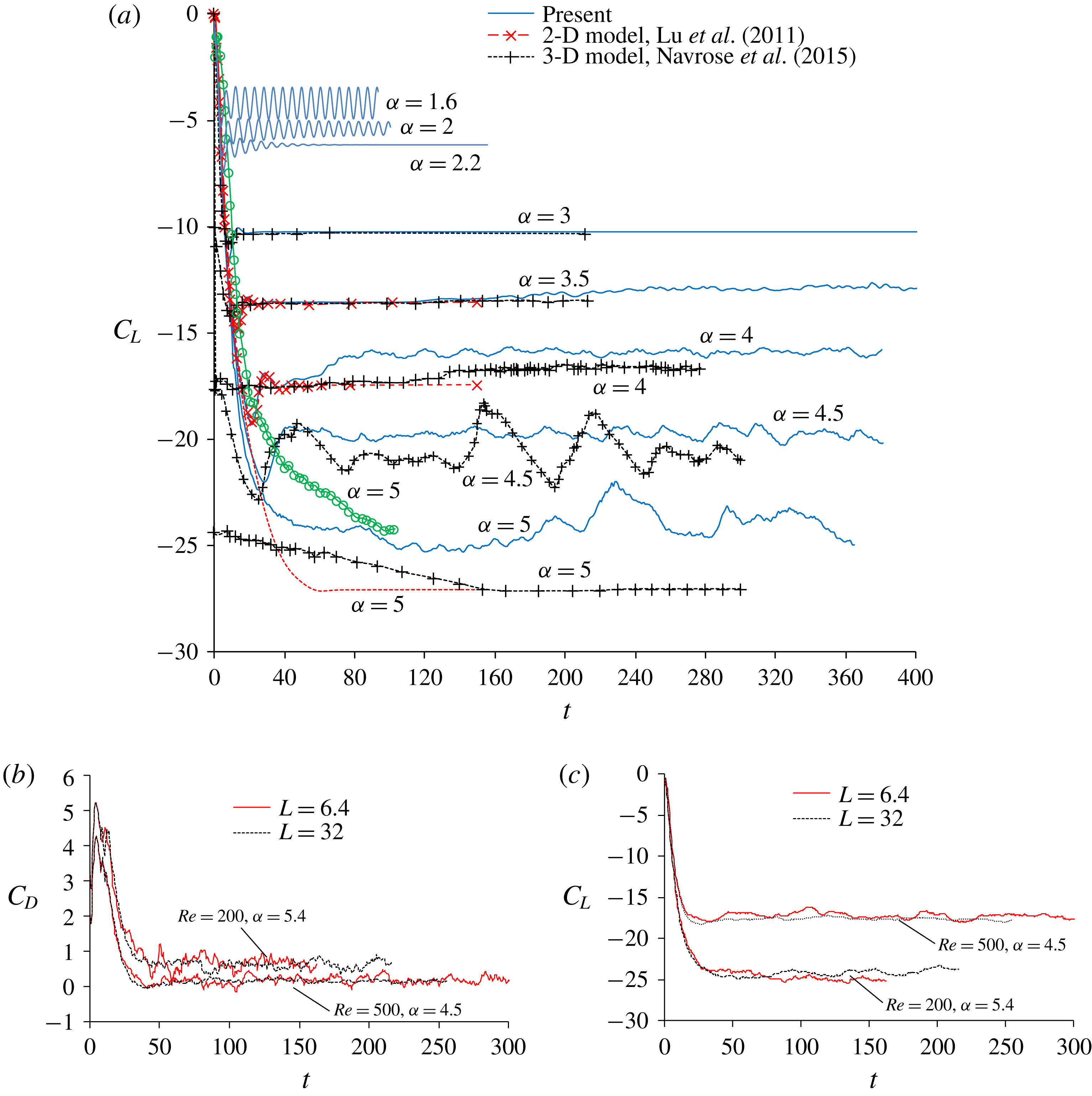
Figure 18(a) shows the selected time histories of the lift coefficient for a range of rotation rates for
 $Re=200$
and their comparison with the 2-D numerical results by Lu et al. (Reference Lu, Qin, Teng and Li2011) and 3-D numerical results by Navrose et al. (Reference Meena and Mittal2015). The lift coefficients are negative due to the Magnus effect caused by the rotation of the cylinder. The 2-D and 3-D numerical results of the lift coefficient for
 $\unicode[STIX]{x1D6FC}\leqslant 3$
are the same because the flow is two-dimensional. The mean lift coefficient at
 $\unicode[STIX]{x1D6FC}=3.5$
and 4.5 in the present numerical study is slightly less than those by Navrose et al. (Reference Meena and Mittal2015). However, the three lift coefficients for
 $\unicode[STIX]{x1D6FC}=5$
in figure 18 are significantly different from each other. The vortex flow is in 3-D RV mode in this study and in Mittal (Reference Mittal2004), who found centrifugal instabilities along the span of the cylinder, while it is found to be in a steady state 2-D flow in Navrose et al. (Reference Meena and Mittal2015). The length-to-diameter aspect ratios of the cylinder used in this study, Mittal (Reference Mittal2004) and Navrose et al. (Reference Meena and Mittal2015) are 6.4, 5 and 12, respectively. Both the lift coefficient and the 3-D flow structure in this study agree with those in Mittal (Reference Mittal2004) because of the similarity of aspect ratio in these two studies.
To see the effects of the cylinder length on the force coefficients, the time histories of the drag and lift coefficients for two cases with strong three-dimensionality of the flow calculated from
 $L=6.4$
and 32 are shown in figures 18(b) and 18(c), respectively. The mean values of drag and lift coefficients for
 $L=6.4$
are very close to their counterparts for
 $L=32$
, respectively, indicating that
 $L=6.4$
is sufficient to obtain satisfactory results for the force coefficients.
(a) Time histories of the lift coefficient together with other numerical results; (b) time histories of drag coefficient for
 $L=6.4$
and 32; (c) time histories of lift coefficient for
 $L=6.4$
and 32.

It is well known that the change in the lift force and vortex shedding patterns are used to identify different flow regimes (Carberry, Sheriden & Rockwell Reference Carberry, Sheriden and Rockwell2001). The lift coefficient oscillates periodically with a constant amplitude at
 $\unicode[STIX]{x1D6FC}=1.6$
as a result of periodic vortex shedding from both sides of the cylinder, as seen in figure 18. The amplitude of the lift coefficient decreases with increasing rotation rate and becomes zero at
 $\unicode[STIX]{x1D6FC}=2.2$
. The amplitude of the lift coefficient remains close to zero until
 $\unicode[STIX]{x1D6FC}=3$
indicating the suppression of vortex shedding. The range of rotation rate from
 $2.2\leqslant \unicode[STIX]{x1D6FC}\leqslant 3$
is in the SS-2D regime. Although, the amplitude of the lift coefficient remains close to zero as
 $\unicode[STIX]{x1D6FC}$
is increased beyond 3, very small oscillations in lift force are observed in the times histories of the lift coefficient of figure 18, which are due to the dynamic motion of ring-shaped and finger-shaped vortices in the wake of the cylinder. It was also shown in figure 7 that, due to the random phases of the sectional lift coefficient along the entire span of the cylinder (mostly out of phase with each other), very weak oscillation of the total lift coefficient is observed at this range of rotation rates. This indicates the inception of very week three-dimensional flow and vortex shedding in the wake of the rotating cylinder. The inception of three-dimensionality of the flow is characterized by the observation of the FV mode. As
 $\unicode[STIX]{x1D6FC}$
exceeds 4.4, the lift coefficient starts to oscillate with large amplitude again until
 $\unicode[STIX]{x1D6FC}=6$
. It is also observed from the time histories of the lift coefficient that the amplitude of the lift coefficient is very irregular inside the RV regime as a result of very chaotic and irregular vortex shedding in this range of rotation rates. The lift coefficient oscillates about a negative mean position throughout the range of rotation rates due the Magnus effect caused by the rotation of the cylinder.
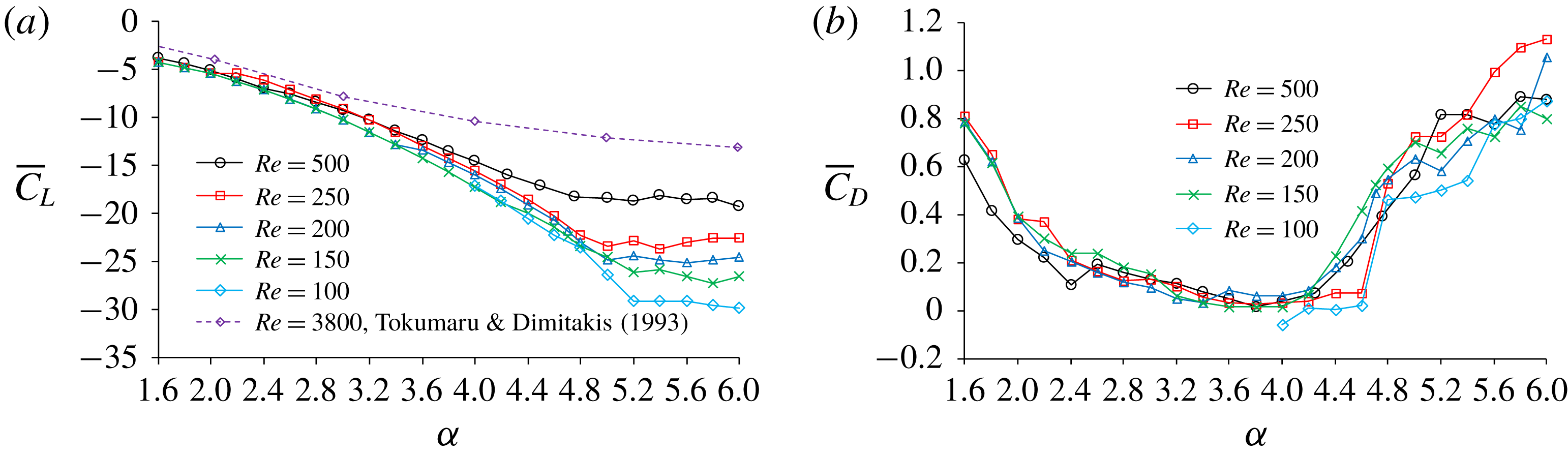
Figure 19(a,b) shows the variations of the mean lift and drag coefficients
 $\overline{C}_{D}$
and
 $\overline{C}_{L}$
(averaged over time) with
 $\unicode[STIX]{x1D6FC}$
. It can be seen that the magnitude of the mean lift coefficient increases with increasing
 $\unicode[STIX]{x1D6FC}$
until some critical value, above which the lift coefficient remains nearly unchanged. Based on potential theory, Prandtl (Reference Prandtl1926) reported that lift coefficient increases with increasing
 $\unicode[STIX]{x1D6FC}$
until it reaches a maximum value of
 $4\unicode[STIX]{x03C0}\approx 12.6$
and stop increasing after then. By conducting experiments, Tokumaru & Dimitakis (Reference Tokumaru and Dimitakis1993) proved Prandtl’s prediction of the existence of a maximum lift coefficient but their experimental maximum lift coefficient is much smaller than the theoretical value based on potential theory. The maximum lift coefficient
 $|\overline{C}_{L}|$
observed in the present study is found to decrease with increasing Reynolds number. It is approximately 30 at
 $Re=100$
and approximately 18.4 at
 $Re=500$
, which is much greater than Tokumaru’s experimental result for
 $Re=3800$
. The mean drag coefficient first decreases with increasing rotation rate and remains close to zero inside the SS-2D mode and FV mode after which there is a profound increase in the drag coefficient with rotation rate inside the RV mode.
Variations of (a) mean lift coefficient and (b) mean drag coefficient with
 $\unicode[STIX]{x1D6FC}$
.

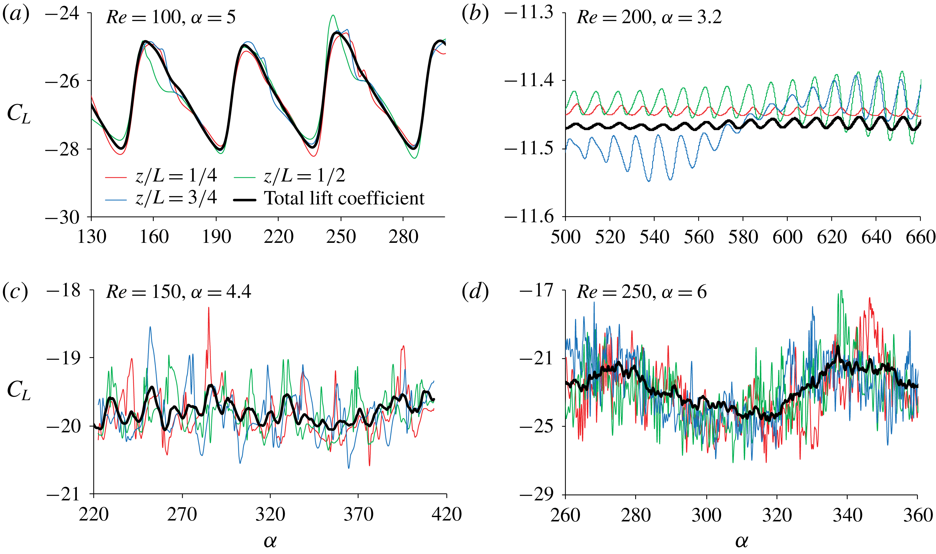
The three-dimensionality of the flow makes the pressure vary along the cylinder span, resulting in strong variation of the force along the cylinder span especially when the three-dimensionality is strong. The difference between the total lift coefficient and the sectional lift coefficient at three locations of
 $z/L=1/4$
,
 $1/2$
and
 $3/4$
for some typical cases can be clearly seen from the time histories of these lift coefficients in figure 20. The total drag and lift coefficients are those calculated based on the total force on the whole cylinder. The flow in the case of
 $Re=100$
and
 $\unicode[STIX]{x1D6FC}=5$
is in the FV regime with weak RVs occurring sporadically along the cylinder span (see the flow pattern in figure 12). It can be seen in figure 20(a) that the sectional lift coefficients in this case are only slightly different from the total force coefficient because the three-dimensionality is weak. The amplitudes of both the sectional and total lift coefficients in the FV regime are small as shown in figure 20(b). The strong difference between the sectional and total lift coefficients in figure 20(c,d), which corresponds to the cases of the RV regime, indicates that the lift coefficients vary significantly along the cylinder span. The strong variation of the lift coefficients along the cylinder span is a direct result of the dynamic motion of the RVs as discussed above.
Comparison between total lift coefficient and sectional lift coefficients at
 $z/L=1/4$
,
 $1/2$
and
 $3/4$
.

The total lift coefficient is essentially the averaged sectional lift coefficient along the cylinder span. The sectional lift coefficient at 65 sections evenly distributed along the cylinder span are calculated and the sectional drag and lift coefficients at
 $k$
th section at time
 $t=n\unicode[STIX]{x0394}t$
are represented as
 $C_{Ds,k}(n\unicode[STIX]{x0394}t)$
and
 $C_{Ls,k}(n\unicode[STIX]{x0394}t)$
, respectively. To quantify the variation of the sectional drag and lift coefficient along the cylinder span, the spatial standard deviation (SD) of the drag and lift coefficients in the spanwise direction (referred to as spanwise SD drag and lift coefficients, respectively, hereafter) are defined as
 $$\begin{eqnarray}C_{Ds}^{\prime \prime }=\left(\frac{1}{65N}\mathop{\sum }_{n=1}^{N}\mathop{\sum }_{k=1}^{65}[C_{Ds,k}(n\unicode[STIX]{x0394}t)-C_{D}(n\unicode[STIX]{x0394}t)]^{2}\right)^{1/2}\end{eqnarray}$$
and
 $$\begin{eqnarray}C_{Ls}^{\prime \prime }=\left(\frac{1}{65N}\mathop{\sum }_{n=1}^{N}\mathop{\sum }_{k=1}^{65}[C_{Ls,k}(n\unicode[STIX]{x0394}t)-C_{L}(n\unicode[STIX]{x0394}t)]^{2}\right)^{1/2},\end{eqnarray}$$
respectively, where
 $C_{D}(n\unicode[STIX]{x0394}t)$
and
 $C_{L}(n\unicode[STIX]{x0394}t)$
are the total drag and lift coefficients, respectively, and
 $n=1$
corresponds to a time when the flow is fully developed. To quantify the oscillation of the sectional drag and lift coefficients in time, the temporal standard derivation of the sectional drag and lift coefficients are defined as
 $$\begin{eqnarray}C_{Ds}^{\prime }=\left(\frac{1}{65N}\mathop{\sum }_{n=1}^{N}\mathop{\sum }_{k=1}^{65}[C_{Ds,k}(n\unicode[STIX]{x0394}t)-\overline{C}_{D}]^{2}\right)^{1/2}\end{eqnarray}$$
and
 $$\begin{eqnarray}C_{Ls}^{\prime }=\left(\frac{1}{65N}\mathop{\sum }_{n=1}^{N}\mathop{\sum }_{k=1}^{65}[C_{Ls,k}(n\unicode[STIX]{x0394}t)-\overline{C}_{L}]^{2}\right)^{1/2}\end{eqnarray}$$
respectively.
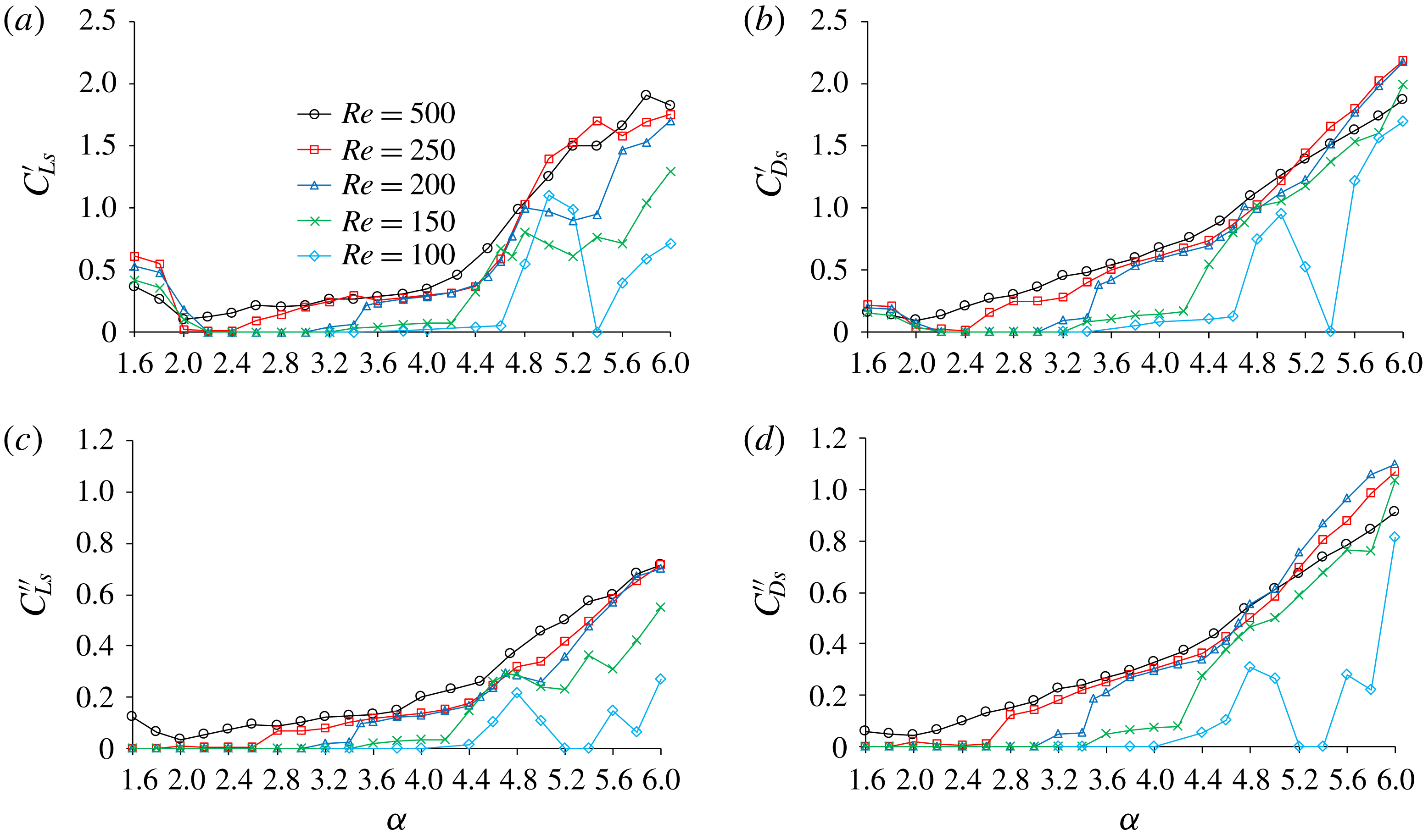
Figure 21 shows variations of the temporal and spanwise SD sectional lift and drag coefficients with the rotation rate
 $\unicode[STIX]{x1D6FC}$
. Generally, there is a sudden change in the SD sectional force coefficients at the boundary of
 $\unicode[STIX]{x1D6FC}$
between two flow regimes. All the SD sectional force coefficients reduce to zero at the boundary of
 $\unicode[STIX]{x1D6FC}$
between VS-2D and SS-2D regimes (for example as
 $\unicode[STIX]{x1D6FC}$
increases from 2 to 2.1 for
 $Re=150$
and 200); whereas, they jump to a non-zero value at the boundary of
 $\unicode[STIX]{x1D6FC}$
between SS-2D and FV (for example as
 $\unicode[STIX]{x1D6FC}$
increases from 3 to 3.2 for
 $Re=200$
). At the boundary between FV and RV regimes, the change rates of SD sectional force coefficients with
 $\unicode[STIX]{x1D6FC}$
increase significantly. The jump in SD force coefficients at the boundary between SS-2D and FV regimes is not observed at
 $Re\geqslant 250$
since the flow SS-2D mode does not exist. In the RV regimes, both the temporal and spanwise SD sectional force coefficients increase with increasing
 $\unicode[STIX]{x1D6FC}$
, except for
 $Re=100$
. It is interesting to see that the temporal SD
 $C_{Ls}^{\prime }$
and
 $C_{Ds}^{\prime }$
for
 $Re=100$
reach their maximum values at
 $\unicode[STIX]{x1D6FC}=5$
, while the spanwise SD
 $C_{Ls}^{\prime \prime }$
and
 $C_{Ds}^{\prime \prime }$
reduce at
 $\unicode[STIX]{x1D6FC}=5$
and reach their minimum values at
 $\unicode[STIX]{x1D6FC}=5.2$
. At
 $Re=100$
, the temporal SD
 $C_{Ls}^{\prime }$
and
 $C_{Ds}^{\prime }$
for
 $\unicode[STIX]{x1D6FC}=4.8$
and 5 are large because the flow is within the secondary instability flow regime (Kang Reference Kang2006), while the very weak three-dimensionality at these two rotation rates leads to significant reduction in the spanwise SD
 $C_{L}^{\prime }$
and
 $C_{D}^{\prime }$
. Since two-dimensional flow is observed at
 $Re=100$
when
 $\unicode[STIX]{x1D6FC}=5.2$
and 5.4, the sectional force coefficients do not oscillate and
 $C_{Ls}^{\prime \prime }$
and
 $C_{Ds}^{\prime \prime }$
become zero. As
 $\unicode[STIX]{x1D6FC}$
exceeds 5.6, the three-dimensionality increases with increasing
 $\unicode[STIX]{x1D6FC}$
(see figure 12) so do the SD force coefficients.
A careful examination of figure 21 reveals that the dependence the SD force coefficient on the Reynolds number is profound for
 $Re\leqslant 200$
and can be correlated very well with the transition between different flow regimes. The SD drag and lift coefficients change significantly at the critical rotation rate where the flow transitions from one regime to another, and the critical rotation rate for the transition of flow regimes is largely dependent on the Reynolds number. High-speed rotation of the cylinder brings about transition to three-dimensional flow at lower Reynolds number compared with the case with a non-rotating cylinder. For
 $Re=100$
and 150, transition of the flow to three-dimensional causes significant increase in SD force coefficients. The increase in the three-dimensionality of flow at higher Reynolds number results in skipping of some flow regimes, for example the SS-2D mode at
 $Re=250$
and the FV mode at
 $Re=500$
. As a result, the SD force coefficients increase with the increase of
 $\unicode[STIX]{x1D6FC}$
almost continuously in the RV regime at higher rotation rates. In the RV regime, the variation trends of the SD force coefficients with the rotation rate for different Reynolds numbers are very similar to each other. There is gradual transition of flow from small RVs to large RVs in the wake of the cylinder inside RV mode which makes the flow chaotic at higher rotation rate and results in an increase in SD force coefficient for all the Reynolds numbers. Although the flow remains turbulent for rotating cylinder like its stationary cylinder counterpart at
 $Re\geqslant 250$
, the flow structures and flow physics are completely different.
Variations of temporal and spanwise sectional lift and drag coefficients with
 $\unicode[STIX]{x1D6FC}$
. (a) Temporal SD sectional lift coefficient. (b) Temporal SD sectional drag coefficient. (c) Spanwise SD sectional lift coefficient. (d) Spanwise SD sectional drag coefficient.

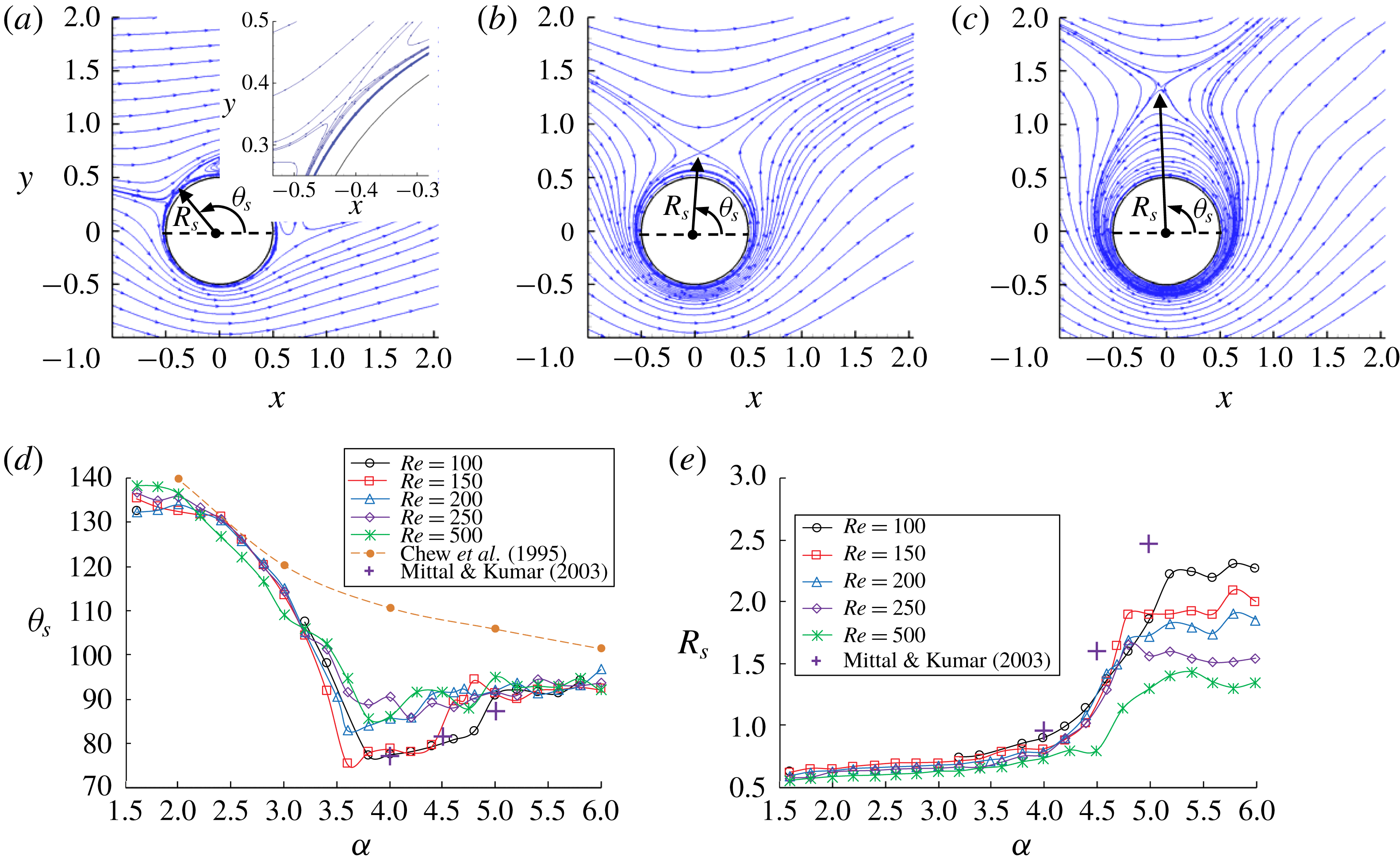
Figure 22(a–c) shows streamlines around the cylinder generated by averaged flow over time and the cylinder span. The position of the stagnation point, which is located on the boundary of the recirculating flow region surrounding the cylinder, is determined by a position angle
 $\unicode[STIX]{x1D703}_{s}$
and the distance between the stagnation point and the centre of the cylinder
 $R_{s}$
shown in figure 22(a–c). The stagnation point is very close to the cylinder surface when
 $\unicode[STIX]{x1D6FC}$
is in the vortex shedding regime (see the zoomed in view at the top right of figure 22
a). It moves away from the cylinder as
 $\unicode[STIX]{x1D6FC}$
increases and the shape of the recirculating flow region become more non-circular.
Figure 22(d,e) shows the variation of the position of the stagnation point with the rotation rate. In figure 22, the data from the results of two-dimensional numerical simulations at
 $Re=1000$
and 200 by Chew et al. (Reference Chew, Cheng and Luo1995) and Mittal & Kumar (Reference Mittal and Kumar2003), respectively, are also plotted for comparison. The values of
 $R_{s}$
and
 $\unicode[STIX]{x1D703}_{s}$
by Mittal & Kumar (Reference Mittal and Kumar2003) are measured from figure 17 in the corresponding reference paper. The quantitative difference between different studies in figure 21 is mainly because two-dimensional models are used in the two previous studies whereas the present study employs three-dimensional numerical simulations. However, the variation trends of
 $R_{s}$
and
 $\unicode[STIX]{x1D703}_{s}$
obtained in the present study are similar to those in the two 2-D studies. The two-dimensional numerical results of
 $\unicode[STIX]{x1D703}_{s}$
for
 $Re=200$
by Mittal & Kumar (Reference Mittal and Kumar2003) are very similar to the present values for
 $Re=100$
and 150, mainly because the three-dimensionality of the flow is very weak at small Reynolds numbers.
The position angle
 $\unicode[STIX]{x1D703}_{s}$
decreases with increasing
 $\unicode[STIX]{x1D6FC}$
in the rotation rate range between 1.6 and 3.5 for all the Reynolds numbers. This causes the reduction of the drag coefficient as shown in figure 19(b). The drag coefficient stops decreasing when the position angle
 $\unicode[STIX]{x1D703}_{s}$
stop reducing with the increase of
 $\unicode[STIX]{x1D6FC}$
at a value between
 $\unicode[STIX]{x1D6FC}=3.5$
and 4. When
 $\unicode[STIX]{x1D6FC}$
exceeds 5, both
 $\unicode[STIX]{x1D703}_{s}$
and
 $R_{s}$
do not change much with the increase of
 $\unicode[STIX]{x1D6FC}$
. This is the reason why the mean lift coefficient in figure 19(a) remains nearly constant as
 $\unicode[STIX]{x1D6FC}$
exceeds 5. The reduction of
 $R_{s}$
with increasing
 $Re$
in the rotation rate range of
 $5\leqslant \unicode[STIX]{x1D6FC}\leqslant 6$
is the evidence that the recirculating flow region shrinks with the increase of
 $Re$
and so does the size of the ring-shaped vortices as discussed above.
Position of the stagnation point. (a) Streamlines for
 $Re=500$
and
 $\unicode[STIX]{x1D6FC}=1.6$
. (b) Streamlines for
 $Re=500$
and
 $\unicode[STIX]{x1D6FC}=4$
. (c) Streamlines for
 $Re=500$
and
 $\unicode[STIX]{x1D6FC}=6$
. (d) Variation of
 $\unicode[STIX]{x1D703}_{s}$
with
 $\unicode[STIX]{x1D6FC}$
. (e) Variation of
 $R_{s}$
with
 $\unicode[STIX]{x1D6FC}$
.

4 Conclusions
The flow structures at
 $Re=200$
are firstly presented because this Reynolds number covers all the flow modes identified. Depending on the rotation rate, different flow regimes are identified based on the flow structures in the wake of the cylinder. It is found that there is a transition from the vortex shedding mode referred to as the VS-2D mode to no vortex shedding mode called the steady state (SS-2D) mode when the rotation rate is increased beyond a critical rotation rate. The flow remains two-dimensional in both these modes. VS-2D mode is characterized by dynamic vortex shedding from both sides of the cylinder. Further increase in rotation rate results in transition to the three-dimensional FV mode, which is characterized by FVs together with extremely weak RVs. As the rotation rate is increased further, the flow enters the RV mode, where the strength of the RVs increases and they wrap the surface of cylinder. Both FVs and RVs are in pairs and the pair number increases with increasing rotation rate.
The formation and motion of FVs and RVs in the FV and RV modes are analysed by observing the vortex motion and pressure distribution on the cylinder surface. In the FV mode, the RVs, which are very weak, are found to oscillate in the spanwise direction with very small amplitudes on the cylinder surface. But the number of RVs does not change and the mean positions of the RVs do not move either. In the FV mode, new RVs are not generated and old RVs do not dissipate. In the RV mode, the RVs become much stronger and the vortex motion is characterized by the continuous generation of new RV pairs from the cylinder surface, which pushes the existing RV pairs outward in the radial direction and the dissipation of old RV pairs as a result of their increasing sizes. Another characteristic of the RV mode is the regrouping of the RV pairs.
The magnitude of the negative mean lift coefficient is found to increase with increasing rotation rate up to a critical rotation rate for all Reynolds numbers, after which it remains constant, which is qualitatively consistent with previous results. The magnitude of the mean lift coefficient is very much dependent on the Reynolds number and is smaller than the one predicted by the potential theory. The mean drag coefficient first decreases with rotation rate and remains almost close to zero inside the SS-2D mode and FV mode after which there is a profound increase in the drag coefficient with rotation rate inside the RV mode. The continuous generation and dissipation of RVs from the cylinder surface in the RV mode causes strong variation of the sectional drag and lift coefficients on the cylinder span, which is proved by the significant increase in the spatial SD of the force coefficients.
The stagnation point is located at the outskirt of the recirculation zone, which is nearly circular when the rotation rate is small and becomes increasingly non-circular as the rotation rate increases. The position angle of the stagnation point decreases with the increase of
 $\unicode[STIX]{x1D6FC}$
until a critical value between
 $\unicode[STIX]{x1D6FC}=3.5$
and 4 for all studied Reynolds numbers. The radius of the stagnation point relative to the cylinder centre decreases with the increase of
 $Re$
in the RV regime, so does the radius of the RVs. In the rotation rate range between 5 and 6, both position angle and radius of stagnation point are nearly independent of
 $\unicode[STIX]{x1D6FC}$
. This is the reason why both the mean drag and lift coefficients remain nearly constant in this range of
 $\unicode[STIX]{x1D6FC}$
.
Acknowledgements
The authors would like to acknowledge the support from the National Key R&D Program of China (Project ID: 2016YFE0200100) and National Natural Science Foundation of China (NSFC) (grant nos. 51628901 and 51779040).