2.1. Governing equations and general solutions

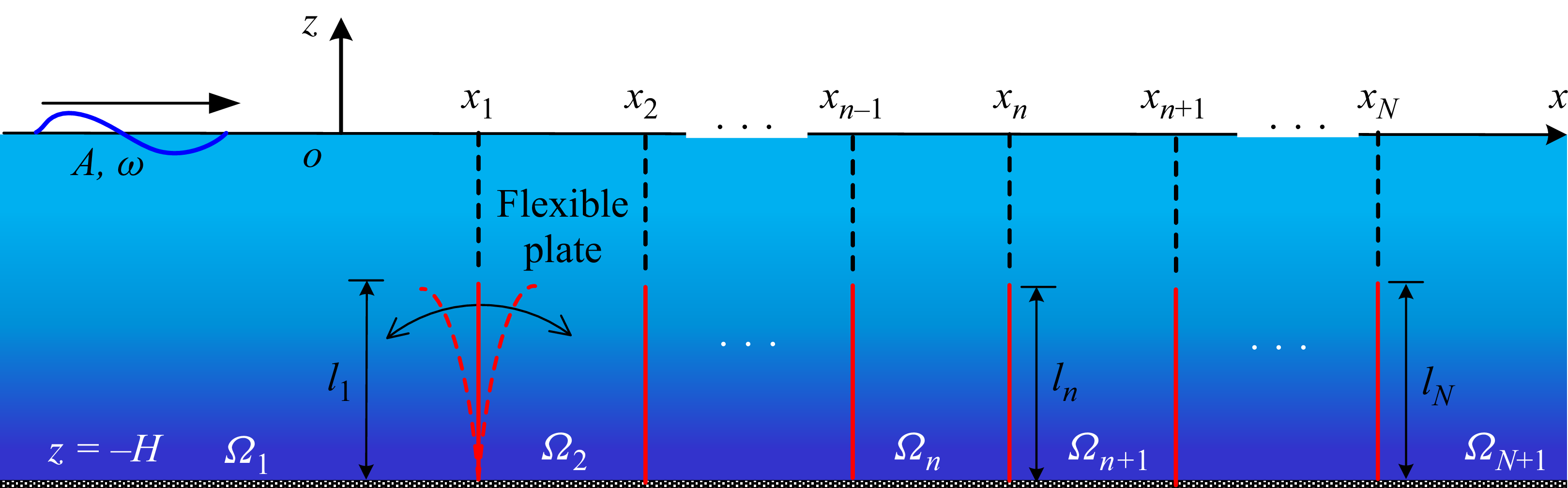
Referring to figure 1, we consider an array of bottom-standing flexible plates embedded in a fluid domain $\varOmega$ of infinite horizontal extent and finite depth $H$ . A two-dimensional Cartesian coordinate system $(x,z)$ is introduced, with the $x$ -axis oriented horizontally, and the $z$ -axis measured vertically upwards. The flat seabed and undisturbed free surface are located at $z=-H$ and $z=0$ , respectively. The array consists of $N$ flexible plates, with the $n$ th plate positioned at $x=x_n$ and extending over the vertical interval $-H \le z \le -d_n$ , where $x_n \in \mathbb{R}$ for $n\in \{1,2,\ldots ,N\}$ , and $l_n=H-d_n$ denotes the plate length, with $d_n$ representing the submergence depth of the plate’s upper edge. From a design perspective, the spacing between adjacent plates ( $x_{n+1} - x_n$ ) must be larger than the sum of their maximum horizontal tip excursions to prevent physical collisions, particularly under resonant conditions where the hydroelastic response is maximised.

Figure 1.

Schematic of an array of flexible plates, oscillating under excitation of the incident wave, forming the so-called metamaterials.

As in many gravity wave problems (Falnes Reference Falnes2002), the fluid is assumed to be inviscid and incompressible, and the motion is taken to be irrotational. Linear wave theory is therefore adopted throughout this work. The velocity field admits a potential representation $\varPhi (x,z,t)=\mathrm{Re} [\phi (x,z)\,\mathrm{e}^{-\mathrm{i}\omega t} ]$ , where $\mathrm{Re}$ denotes the real part, $\phi$ is the complex-valued spatial velocity potential, $\omega$ is the angular frequency, and $\mathrm{i}=\sqrt {-1}$ is the imaginary unit. In the same spirit, the motion of each flexible plate is assumed to be harmonic and linear, so that the transverse deflection of the $n$ th plate can be written as $W_n(z,t)=\mathrm{Re} [w_n(z)\,\mathrm{e}^{-\mathrm{i}\omega t} ]$ .

2.1.1. Flexible plate

We begin with the structural dynamics of the flexible plates. The plates are taken to be slender and free of shear deformation, and are thus modelled as Euler–Bernoulli beams in the present two-dimensional setting. The linearised equation of motion of the $n$ th plate reads

(2.1) \begin{equation} E_nI_n\,\partial _z^4 w_n-\omega ^2\rho _n b_n w_n = \mathrm{i}\omega \rho _w\big (\phi |_{x=x_n^-}-\phi |_{x=x_n^+}\big ), \end{equation}

where $E_n$ is the Young’s modulus of the plate, $b_n$ is its thickness, $I_n=b_n^3/12$ is the second moment of area, $\rho _n$ is the plate density, and $\rho _w$ is the water density. Here, $x_n^-$ and $x_n^+$ denote the fluid point immediately to the left and right of the plate, respectively. The left-hand side of (2.1) represents the intrinsic structural response, arising from bending stiffness and inertia, whereas the right-hand side accounts for the hydrodynamic forcing induced by the pressure jump across the plate.

To solve for the structural deformation, the mode expansion method is employed, and the plate displacement is expanded as

(2.2) \begin{equation} w_n(z)=\sum _{m=1}^{\infty }\sigma _{n,m}\,w_{n,m}(z), \end{equation}

where $w_{n,m}(z)$ is the $m$ th natural mode of the $n$ th plate, and $\sigma _{n,m}$ is the corresponding complex modal amplitude. Each mode shape satisfies

(2.3) \begin{equation} \partial _z^4w_{n,m}- (\kappa _{n,m})^4\,w_{n,m}(z)=0, \end{equation}

with $ (\kappa _{n,m} )^4= (\omega _{n,m} )^2\rho _nb_n/(E_nI_n)$ , and $\omega _{n,m}$ denoting the associated eigenfrequency.

The clamped lower edge at the seabed and the free upper edge of the plate impose the boundary conditions

(2.4a) \begin{equation} w_{n,m}\big |_{z=-H}=\partial _z w_{n,m}\big |_{z=-H}=0, \end{equation}

(2.4b) \begin{equation} \partial _z^2 w_{n,m}\big |_{z=-d_n}=\partial _z^3 w_{n,m}\big |_{z=-d_n}=0. \end{equation}

The governing equation (2.3), together with the boundary conditions (2.4), yields the mode shape

(2.5) \begin{equation} \begin{aligned} w_{n,m}(z)=\,&\cos \!\left [\kappa _{n,m}(z+H)\right ] -\cosh \!\left [\kappa _{n,m}(z+H)\right ] \\[3pt] &-\xi _{n,m}\left \{ \sin \!\left [\kappa _{n,m}(z+H)\right ] -\sinh \!\left [\kappa _{n,m}(z+H)\right ] \right \}\!, \end{aligned} \end{equation}

where

(2.6) \begin{equation} \xi _{n,m}= \frac {\cos \!\left (\kappa _{n,m}l_n\right )+\cosh \!\left (\kappa _{n,m}l_n\right )} {\sin \!\left (\kappa _{n,m}l_n\right )+\sinh \!\left (\kappa _{n,m}l_n\right )} \ , \end{equation}

and $\kappa _{n,m}$ is determined by

(2.7) \begin{equation} \cos \!\left (\kappa _{n,m}l_n\right )\cosh \!\left (\kappa _{n,m}l_n\right )+1=0. \end{equation}

Having established the modal basis, we project the governing equation onto each mode. Multiplying (2.1) by $w_{n,\zeta }(z)$ and integrating over $[-H,-d_n]$ , and then invoking the orthogonality of the natural modes, gives

(2.8) \begin{equation} \sigma _{n,\zeta }\big (E_n I_n \kappa _{n,\zeta }^{4}-\omega ^{2}\rho _n b_n\big)l_n = F_{n,\zeta }, \end{equation}

where

(2.9) \begin{equation} F_{n,\zeta }=-\mathrm{i}\omega \rho _w \int _{-H}^{-d_n}\Delta \phi _n(z)\,w_{n,\zeta }(z)\,\mathrm{d}z \end{equation}

represents the hydrodynamic force acting on plate $n$ in mode $\zeta$ , and

(2.10) \begin{equation} \Delta \phi _n(z)=\phi (x_n^{+},z)-\phi (x_n^{-},z) \end{equation}

denotes the potential jump across the plate.

The principal mass and principal stiffness of the flexible plate are defined as

(2.11a) \begin{align} M_{n,m}&=\int _{-H}^{-d_n}\rho _n b_n\left [w_{n,m}(z)\right ]^2\,\mathrm{d}z = l_n\rho _n b_n, \\[-12pt]\nonumber \end{align}

(2.11b) \begin{align} K_{n,m}&=\int _{-H}^{-d_n}E_nI_n\left [w_{n,m}^{\prime \prime }(z)\right ]^2\,\mathrm{d}z = \kappa _{n,m}^{4}l_nE_nI_n. \end{align}

Accordingly, (2.1) can be recast in the compact form

(2.12) \begin{equation} \sigma _{n,\zeta }\big (K_{n,\zeta }-\omega ^{2}M_{n,\zeta }\big )=F_{n,\zeta }. \end{equation}

2.1.2. Fluid problem

We now turn to the fluid problem. The water motion is described by linear potential flow theory, such that the velocity field is given by the gradient of the scalar potential $\phi$ , which satisfies Laplace’s equation in the fluid domain:

(2.13) \begin{equation} \boldsymbol{\nabla} ^{2}\phi =0 \quad \text{for all } (x,z)\in \varOmega . \end{equation}

At the free surface, the linearised dynamic and kinematic conditions yield

(2.14) \begin{equation} \partial _{z}\phi =\frac {\omega ^{2}}{g}\phi \quad \text{at } \quad z=0, \end{equation}

while the impermeable seabed imposes

(2.15) \begin{equation} \partial _{z}\phi =0 \quad \text{on } \quad z=-H. \end{equation}

On the wetted surface of plate $n$ , the kinematic condition enforces continuity of normal velocity:

(2.16) \begin{equation} \partial _{x}\phi =-\mathrm{i}\omega w_n(z) \quad \text{for } \quad (x,z)\in \varGamma _n^{p}, \end{equation}

where $\varGamma _n^{p}=\{(x_n,z)\,|\, {-H}\lt z\lt -d_n\}$ denotes the submerged portion of plate $n$ .

Substituting the modal expansion of $w_n$ yields

(2.17) \begin{equation} \partial _x\phi = -\mathrm{i}\omega \sum _{m=1}^{\infty }\sigma _{n,m}\,w_{n,m}(z), \end{equation}

thereby coupling the fluid motion directly to the structural modes.

Using separation of variables, the general solution of (2.13), subject to the boundary conditions (2.14)–(2.15), can be expressed as

(2.18) \begin{equation} \phi (x,z)= \sum _{j=0}^{\infty } \big ( B_{\!j}\, \mathrm{e}^{k_{\!j} x} + C_{\!j}\, \mathrm{e}^{-k_{\!j} x} \big) Z_{\!j}(z) \quad \text{for all }(x,z)\in \varOmega , \end{equation}

where $B_{\!j}$ and $C_{\!j}$ are undetermined coefficients, and $k_{\!j}$ are the positive roots of the dispersion relation

(2.19) \begin{equation} \omega ^2/g+k_{\!j}\tan (k_{\!j} H)=0, \quad j\in \mathbb{N}^{+}\cup \{0\}. \end{equation}

Here, $k_0=-\mathrm{i}k$ corresponds to the progressive wave mode, whereas $k_{\!j}\in \mathbb{R}^{+}$ for $j\gt 0$ corresponds to the evanescent modes.

The associated vertical eigenfunctions are given by (Mei Reference Mei1992)

(2.20) \begin{equation} Z_{\!j}(z)=\frac {1}{\sqrt {N_{\!j}}}\cos \!\left [k_{\!j}(H+z)\right ], \end{equation}

where

(2.21) \begin{equation} N_{\!j}=\frac {\sin (2k_{\!j} H)}{4k_{\!j} H}+\frac {1}{2} \end{equation}

is the normalisation constant, chosen such that the eigenfunctions satisfy

(2.22) \begin{equation} \int _{-H}^{0} Z_{\!j}(z)\,Z_{\zeta }(z)\,\mathrm{d}z =H\delta _{j,\zeta } \end{equation}

for all $j,\zeta \in \{0\}\cup \mathbb{N}^{+}$ .

To account for the edge singularity in the vicinity of the plate tips, the Galerkin method is employed so as to incorporate both the vanishing potential jump and the square-root velocity behaviour near the plate edges (Porter & Evans Reference Porter and Evans1995). An auxiliary function is introduced to represent the horizontal velocity in the gap above submerged plate $n$ :

(2.23) \begin{equation} U_n(z)=\sum _{q=0}^{\infty }U_{n,q}\,u_{n,q}(z) \quad \text{for } \quad (x,z)\in \varGamma _n^{G}, \end{equation}

where $\varGamma _n^{G}=\{(x_n,z)\,|\, {-d_n}\lt z\lt 0\}$ denotes the gap region, and $U_{n,q}$ are unknown coefficients.

The auxiliary basis functions are chosen to satisfy the free-surface condition and the convergence requirement at the edge $(x_n,-d_n)$ . Thus $u_{n,q}(z)$ is defined by

(2.24) \begin{equation} u_{n,q}(z) - \frac {\omega ^2}{g} \int _{-d_n}^{0} u_{n,q}(t)\,\mathrm{d}t = \frac {2(-1)^q}{\pi \sqrt {d_n^2-z^2}} \,T_{2q}\!\left (\frac {z}{d_n}\right )\!, \end{equation}

where $T_{2q}$ is the Chebyshev polynomial of the first kind of degree $2q$ .

2.2. Finite array of flexible plates

2.2.1. Wave motion

We consider a finite-sized FPMM assembly comprising $N$ periodically arranged unit cells, as schematically illustrated in figure 1. A monochromatic incident wave train propagates along the positive $x$ -direction, inducing hydroelastic oscillations of the flexible plates. Within the framework of linearised potential flow theory, the total velocity potential $\phi (x, z)$ can be partitioned into the incident potential $\phi ^I$ , the diffraction potential $\phi ^D$ (associated with the fixed structures), and the radiation potentials $\phi ^{R,n,m}$ resulting from the modal oscillations of the plates. Specifically, the decomposition is expressed as

(2.25) \begin{equation} \phi = \phi ^I + \phi ^D + \sum _{n=1}^N \sum _{m=1}^\infty \dot {\sigma }_{n,m} \phi ^{R,n,m}, \end{equation}

where $\dot {\sigma }_{n,m} = -\mathrm{i} \omega \sigma _{n,m}$ represents the complex velocity amplitude of the $n$ th flexible plate oscillating in its $m$ th natural mode. The radiation potential $\phi ^{R,n,m}$ corresponds to the wave field generated by the $m$ th mode of the $n$ th plate in otherwise calm water.

The incident potential for a regular wave of amplitude $A$ and angular frequency $\omega$ is defined by

(2.26) \begin{equation} \phi ^I = -\frac {\mathrm{i}gA}{\omega } \frac {\cosh [k(z + H)]}{\cosh (kH)}\, \mathrm{e}^{\mathrm{i}kx}, \end{equation}

where the wavenumber $k$ is the positive real root of the linear dispersion relation at water depth $H$ :

(2.27) \begin{equation} \omega ^2/g = k \tanh (kH). \end{equation}

The unknown potentials $\phi ^D$ and $\phi ^{R,n,m}$ are governed by the Laplace equation within the fluid domain, subject to the standard free-surface and seabed boundary conditions. The kinematic boundary conditions on the surfaces of the plates $\varGamma _n^P$ for a given potential $\phi ^\chi$ ( $\chi \in \{D, (R,n,m)\}$ ) are stipulated as

(2.28) \begin{equation} \partial _x \phi ^\chi = \begin{cases} -\partial _x \phi ^I, & \chi = D \\[3pt] \delta _{n,i}\, w_{n,m}(z), & \chi = (R,n,m) \end{cases} \quad \text{for } \quad (x,z) \in \varGamma _n^P, \end{equation}

where $\delta _{n,i}$ denotes the Kronecker delta, signifying that for the radiation problem, only the $n$ th plate is in motion. To ensure the uniqueness of the solution, the Sommerfeld radiation condition is imposed at infinity, requiring the scattered waves to be purely outgoing:

(2.29) \begin{equation} \lim _{x \to \pm \infty } \big ( \partial _x \phi ^\chi \mp \mathrm{i}k \phi ^\chi \big) = 0. \end{equation}

The boundary-value problem is solved using the matched eigenfunction expansion method. The fluid domain $\varOmega$ is partitioned into $N+1$ subdomains: the semi-infinite upstream region $\varOmega _1$ , the interior regions between adjacent plates $\varOmega _n$ ( $n=2, \ldots , N$ ), and the semi-infinite downstream region $\varOmega _{N+1}$ , as depicted in figure 1. By invoking the separation of variables and satisfying the radiation conditions (2.29), the general solution for the diffracted and radiated velocity potential in each region is expanded as follows:

(2.30a) \begin{align} \phi _1^\chi &= \sum _{j=0}^\infty B_{1,j}^\chi\, \mathrm{e}^{k_{\!j} x}\, Z_{\!j}(z), \quad (x,z) \in \varOmega _1, \\[-12pt]\nonumber \end{align}

(2.30b) \begin{align} \phi _n^\chi &= \sum _{j=0}^\infty \big ( B_{n,j}^\chi\, \mathrm{e}^{k_{\!j} x} + C_{n,j}^\chi\, \mathrm{e}^{-k_{\!j} x} \big) Z_{\!j}(z), \quad (x,z) \in \varOmega _n \ (n=2,\ldots ,N), \\[-12pt]\nonumber \end{align}

(2.30c) \begin{align} \phi _{N+1}^\chi &= \sum _{j=0}^\infty C_{N+1,j}^\chi\, \mathrm{e}^{-k_{\!j} x}\, Z_{\!j}(z), \quad (x,z) \in \varOmega _{N+1}, \end{align}

where $Z_{\!j}(z)$ are the vertical eigenfunctions, and $k_{\!j}$ are the corresponding eigenvalues. The coefficients $B_{n,j}^\chi$ and $C_{n,j}^\chi$ are to be determined by invoking the continuity of pressure and horizontal velocity across the fluid interfaces at $x=x_n$ . By exploiting the orthogonality of the eigenfunctions, the matching conditions are transformed into a truncated system of linear algebraic equations. The detailed algebraic procedure is relegated to Appendix A.

2.2.2. Structural motion

The dynamic response of the finite FPMM is governed by the structural equations of motion. For each resonator, the modal displacement amplitudes $\sigma _{n,m}$ are coupled with the fluid field via the hydrodynamic pressure. According to the modal expansion technique, the generalised wave force acting on the $n$ th plate in its $\zeta$ th mode is expressed as

(2.31) \begin{equation} F_{n,\zeta } = -\mathrm{i} \omega \rho _w \int _{-H}^{-d_n} \Delta \phi _n(z)\, w_{n,\zeta }(z)\, \mathrm{d}z = F_{n,\zeta }^e - \mathrm{i} \omega \sum _{p=1}^{N} \sum _{L=1}^{\infty } f_{n,\zeta }^{s,o} \sigma _{s,o}, \end{equation}

where $F_{n,\zeta }^e$ represents the wave excitation force due to the diffraction of waves by the fixed array,

(2.32) \begin{equation} F_{n,\zeta }^e = \mathrm{i} \omega \rho _w \int _{-H}^{-d_n} \left ( \left . \phi ^D \right |_{x=x_n^-} - \left . \phi ^D \right |_{x=x_n^+} \right ) w_{n,\zeta }(z)\, \mathrm{d}z, \end{equation}

and $f_{n,\zeta }^{s,o}$ signifies the generalised radiation force on mode $\zeta$ of plate $n$ caused by the unit-velocity oscillation of mode $o$ of plate $s$ . The radiation force is conventionally decomposed into added mass $a_{n,\zeta }^{s,o}$ and radiation damping $c_{n,\zeta }^{s,o}$ coefficients:

(2.33) \begin{equation} f_{n,\zeta }^{s,o} = \mathrm{i} \omega a_{n,\zeta }^{s,o} - c_{n,\zeta }^{s,o}. \end{equation}

By truncating the modal expansion at a sufficiently large order $M$ , the coupled hydroelastic system can be cast into a compact matrix form,

(2.34) \begin{equation} \big [ -\omega ^2(\boldsymbol{M}_{\!s} + \boldsymbol{a}) - \mathrm{i} \omega \boldsymbol{c} + \boldsymbol{K} \big ] \boldsymbol{X} = \boldsymbol{F}_{\!\boldsymbol{e}}, \end{equation}

where $\boldsymbol{X}$ and $\boldsymbol{F}_{\!e}$ are the vectors of modal responses and excitation forces, respectively. The matrices $\boldsymbol{M}_{\!s}$ and $\boldsymbol{K}$ represent the intrinsic modal mass and stiffness of the plates, while $\boldsymbol{a}$ and $\boldsymbol{c}$ are the global added-mass and radiation damping matrices, capturing the hydrodynamic coupling between all resonators:

(2.35a,b) \begin{align} \boldsymbol{a} = [a_{n,m}^{s,o}]_{\textit{NM} \times \textit{NM}}, \quad \boldsymbol{c} = [c_{n,m}^{s,o}]_{\textit{NM} \times \textit{NM}}. \end{align}

The solution to (2.34) yields the structural response, from which the complete wave field is reconstructed via (2.25).

2.2.3. Reflection and transmission coefficients

The far-field performance of the FPMM array is characterised by the reflection ( $R$ ) and transmission ( $T$ ) coefficients. Based on the linearised free-surface condition, the wave elevation is given by $\eta = (\mathrm{i}\omega /g) \phi |_{z=0}$ . In the asymptotic limit as $x \to \pm \infty$ , only the propagating modes ( $j=0$ ) contribute to the wave elevation. Consequently, the coefficients are derived from the complex amplitudes of the reflected and transmitted waves:

(2.36a) \begin{align} R &= \left | \frac {\mathrm{i} \omega\, Z_0(0)}{gA} \left ( B_{1,0}^D + \sum _{n=1}^N \sum _{m=1}^M \dot {\sigma }_{n,m} B_{1,0}^{R,n,m} \right ) \right |\!, \\[-12pt]\nonumber \end{align}

(2.36b) \begin{align} T &= \left | 1 + \frac {\mathrm{i} \omega\, Z_0(0)}{gA} \left ( C_{N+1,0}^D + \sum _{n=1}^N \sum _{m=1}^M \dot {\sigma }_{n,m} C_{N+1,0}^{R,n,m} \right ) \right |\!. \end{align}

For this non-dissipative potential flow problem, the energy conservation principle $R^2 + T^2 = 1$ is employed to verify the numerical consistency and convergence of the implemented method.

2.3. Infinite array of flexible plates

To elucidate the fundamental wave-steering properties and the emergence of bandgaps in the FPMM, we now extend the formulation to an infinitely periodic assembly of flexible plates along the $x$ -axis. By invoking the discrete translational symmetry of the system, the analysis can be elegantly reduced to a single representative unit cell of length $L$ . In accordance with the solution form established in § 2.2, the velocity potential in the fluid domains adjacent to the $n$ th plate is represented as

(2.37) \begin{equation} \phi _n = \sum _{j=0}^{\infty } \big ( B_{n,j}\, \mathrm{e}^{k_{\!j} x} + C_{n,j}\, \mathrm{e}^{-k_{\!j} x} \big ) Z_{\!j}(z), \quad (x,z) \in \varOmega _n, \end{equation}

(2.38) \begin{equation} \phi _{n+1} = \sum _{j=0}^{\infty } \big ( B_{n+1,j}\, \mathrm{e}^{k_{\!j} x} + C_{n+1,j}\, \mathrm{e}^{-k_{\!j} x} \big ) Z_{\!j}(z), \quad (x,z) \in \varOmega _{n+1}, \end{equation}

where $B_{n,j}, C_{n,j}$ and $B_{n+1,j}, C_{n+1,j}$ are the modal coefficients to be determined via the interfacial matching conditions.

Across the vertical interface at $x=x_n$ , the continuity of the horizontal velocity and the pressure must be satisfied. The kinematic boundary condition, accounting for both the fluid gap and the hydroelastic motion of the plate, is given by

(2.39) \begin{equation} \left . \partial _x \phi _n \right |_{x=x_n} = \left . \partial _x \phi _{n+1} \right |_{x=x_n} = \begin{cases} U_n(z), & (x,z) \in \varGamma _n^G, \\[3pt] -\mathrm{i} \omega \sum _{m=1}^{\infty } \sigma _{n,m}\, w_{n,m}(z), & (x,z) \in \varGamma _n^P, \end{cases} \end{equation}

(2.40) \begin{equation} \left . \phi _n \right |_{x=x_n} = \left . \phi _{n+1} \right |_{x=x_n}, \quad (x,z) \in \varGamma _n^G. \end{equation}

To decouple the structural response from the fluid problem, the modal displacement $\sigma _{n,m}$ is expressed in terms of the potential jump $\Delta \phi _n$ by rearranging the dynamic equations (2.9) and (2.12):

(2.41) \begin{equation} \sigma _{n,m} = \frac {-\mathrm{i} \omega \rho _w \int _{-H}^{-d_n} \Delta \phi _n(z)\, w_{n,m}(z)\, \mathrm{d}z}{K_{n,m} - \omega ^2 M_{n,m}}. \end{equation}

The spatial periodicity of the infinite lattice allows the application of Bloch’s theorem (or Floquet theory). This theorem stipulates that the wave field in the $(n+1)$ th cell is related to that in the $n$ th cell via a complex phase modulation

(2.42) \begin{equation} \phi (x + L, z) = \mathrm{e}^{\mathrm{i} p L}\, \phi (x, z), \end{equation}

where $p$ denotes the Bloch wavenumber. Due to the reciprocal nature of the lattice, the first Brillouin zone $p \in [0, \pi /L]$ is sufficient to characterise the dispersion properties. Consequently, the potential in the domain $\varOmega _{n+1}$ can be mapped from the domain $\varOmega _n$ as

(2.43) \begin{equation} \phi _{n+1} = \mathrm{e}^{\mathrm{i} p L} \sum _{j=0}^{\infty } \big ( B_{n,j}\, \mathrm{e}^{k_{\!j} (x-L)} + C_{n,j}\, \mathrm{e}^{-k_{\!j} (x-L)} \big) Z_{\!j}(z), \quad (x,z) \in \varOmega _{n+1} . \end{equation}

Substituting the periodic representations (2.37) and (2.43) into the continuity requirements (2.39) and (2.40), and projecting the resulting equations onto the orthogonal basis $Z_{\!j}(z)$ , we obtain a system of governing equations for the unit cell. This formulation leads to a global homogeneous system of the form

(2.44) \begin{equation} \boldsymbol{S}(\omega , p)\, \boldsymbol{x} = \mathbf{0}, \end{equation}

where $\boldsymbol{x}$ is the vector of unknown coefficients defined as

(2.45) \begin{equation} \boldsymbol{x} = \big[ B_{n,0}, \ldots , B_{n,J}, C_{n,0}, \ldots , C_{n,J}, U_{n,0}, \ldots , U_{n,Q} \big]^{\mathrm{T}}. \end{equation}

The transcendental coefficient matrix $\boldsymbol{S}$ encapsulates the hydroelastic coupling and the Bloch periodicity:

(2.46) \begin{equation} \boldsymbol{S} = \begin{bmatrix} S_{1,B}^{v,l} + S_{4,B}^{v} - \alpha S_{3,B}^{v} & S_{1,C}^{v,l} + S_{4,C}^{v} - \alpha S_{3,C}^{v} & -S_{2}^{v} \\[9pt] \alpha \big(S_{1,B}^{v,r} - S_{3,B}^{v}\big) + S_{4,B}^{v} & \alpha \big(S_{1,C}^{v,r} - S_{3,C}^{v}\big) + S_{4,C}^{v} & -S_{2}^{v} \\[9pt] S_{1,B}^{p} - \alpha S_{2,B}^{p} & S_{1,C}^{p} - \alpha S_{2,C}^{p} & \mathbf{0} \end{bmatrix} \end{equation}

where the constitutive sub-matrices are detailed in Appendix B.

The dispersion relation $\omega (p)$ is implicitly defined by the existence of non-trivial solutions to (2.44), requiring the vanishing of the determinant

(2.47) \begin{equation} \mathcal{D}(\omega , p) = \mathrm{det}[\boldsymbol{S}(\omega , p)] = 0. \end{equation}

For a prescribed real frequency $\omega$ , the roots $p$ are generally complex. A purely real $p$ corresponds to a propagating Bloch mode, signifying a passband, whereas a complex $p$ with a non-zero imaginary part indicates spatial attenuation (evanescent modes), characterising the presence of a spectral bandgap.

3.1. The LR mechanism

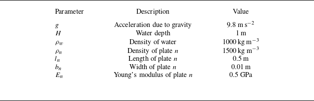
In this subsection, we elucidate the fundamental dynamic characteristics of the FPMM by first examining the probative case of a solitary resonator interacting with monochromatic waves. The structural and fluid parameters prescribed for this canonical configuration are summarised in table 1.

Table 1.

Geometric and material properties of the fluid domain and the flexible plate. Note that each plate in the array has the same parameter values. Unless otherwise specified, these parameters remain constant throughout § 3.

Table 1. Long description

A table with three columns and eight rows. The columns are labeled Parameter, Description, and Value. The rows list the parameters, their descriptions, and corresponding values. Row 1: Parameter: g, Description: Acceleration due to gravity, Value: 9.8 m s^-2. Row 2: Parameter: H, Description: Water depth, Value: 1 m. Row 3: Parameter: ρw, Description: Density of water, Value: 1000 kg m^-3. Row 4: Parameter: ρn, Description: Density of plate n, Value: 1500 kg m^-3. Row 5: Parameter: ln, Description: Length of plate n, Value: 0.5 m. Row 6: Parameter: bn, Description: Width of plate n, Value: 0.01 m. Row 7: Parameter: En, Description: Young’s modulus of plate n, Value: 0.5 GPa.

Figure 2.

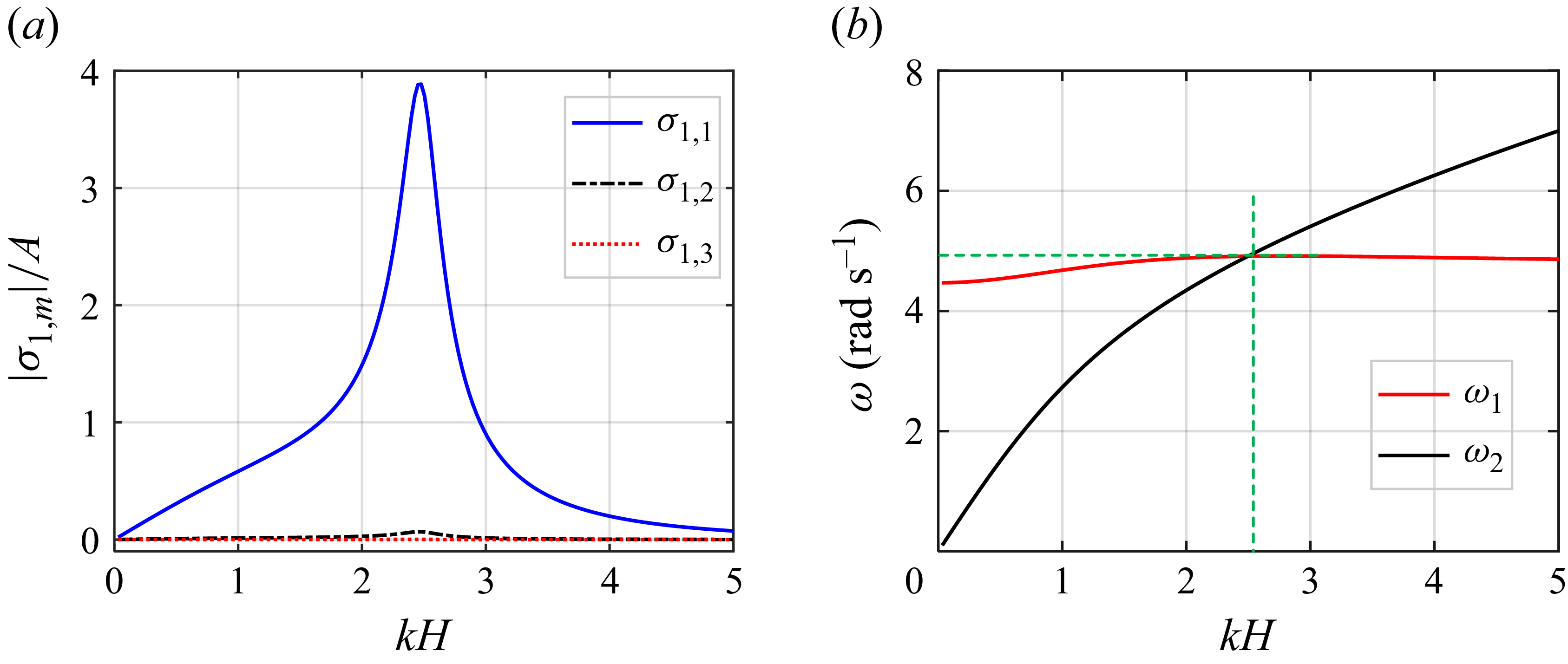
(a) Modal amplitude distributions of the first three elastic modes. (b) Graphical determination of the resonance frequency of the submerged flexible resonator.

The spectral response of the flexible plate, characterised by the amplitudes of the first three elastic modes, is depicted in figure 2(a). It is manifest that the first-order mode ( $\sigma _{1,1}$ ) dominates the structural dynamics within the frequency range of interest, whereas higher-order modal contributions ( $\sigma _{1,2}, \sigma _{1,3}$ ) remain negligible. This modal hierarchy not only confirms the rapid convergence of our analytical solution, but also justifies the truncation at $M=3$ for the subsequent parametric studies.

Determining the effective natural frequency of the resonator submerged in fluid necessitates accounting for the frequency-dependent hydrodynamic loading, specifically the added mass $a_{1,1}^{1,1}(\omega )$ . Unlike a structure vibrating in a vacuum where the natural frequency remains static, the submerged flexible plate experiences frequency-dependent hydrodynamic added mass induced by the surrounding fluid. To identify the true resonant state of this coupled fluid–structure system, we employ a graphical approach as illustrated in figure 2(b). Here, the curve $\omega _1 = [K_{1,1} / (M_{1,1} + a_{1,1}^{1,1}(\omega ))]^{1/2}$ represents the ‘wet’ natural frequency of the first-order structural mode (where the generalised modal mass $M_{1,1}$ and stiffness $K_{1,1}$ are defined via (2.11)), while the curve $\omega _2 = [gk \tanh (kH)]^{1/2}$ denotes the inherent dispersion relation of the water waves. Curves $\omega _1$ and $\omega _2$ create an intersection, where the ordinate corresponds to the resonator’s natural frequency, and the abscissa represents the corresponding dimensionless wavenumber. The equilibrium point is found at $\omega = 4.85\ \text{rad}\ \text{s}^{-1}$ (corresponding to a dimensionless wavenumber $kH = 2.45$ ), which precisely aligns with the peak modal amplitude observed in figure 2(a).

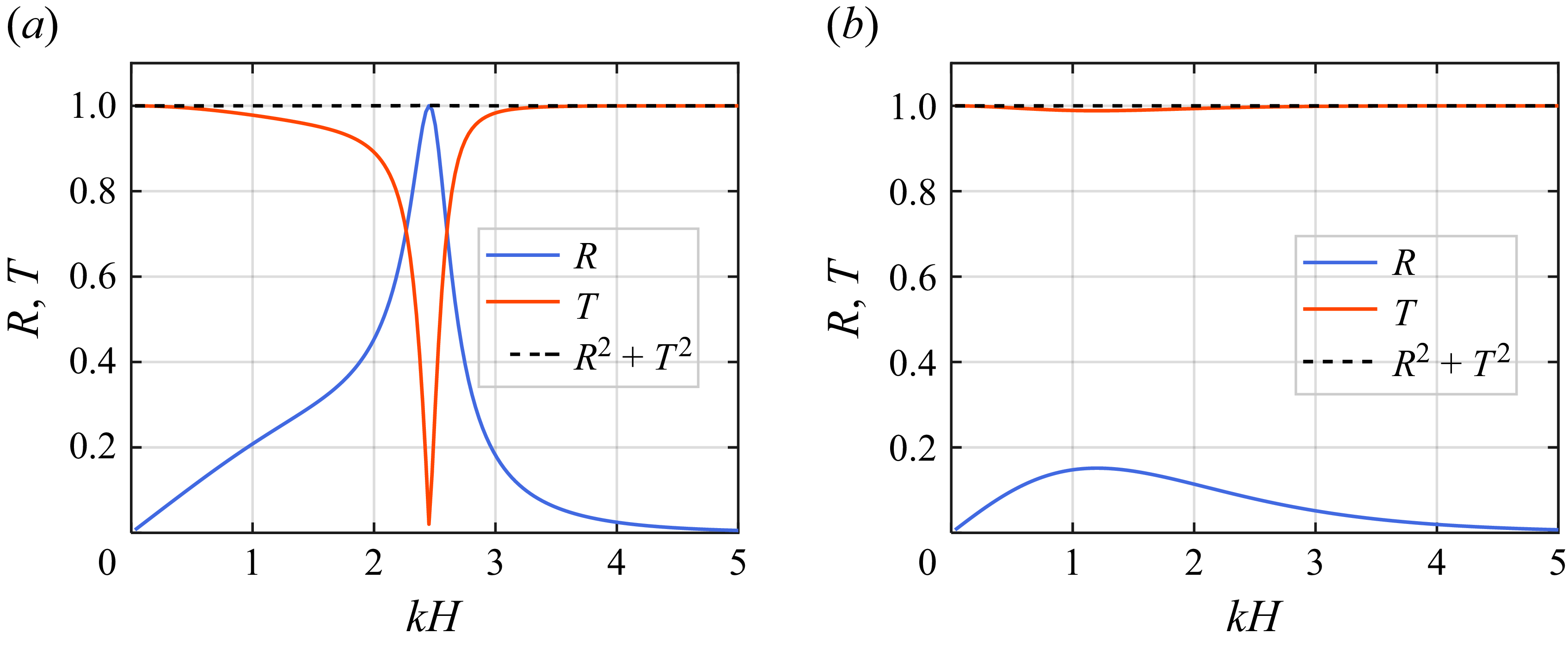
The scattering performance of the resonator is quantified by the reflection ( $R$ ) and transmission ( $T$ ) coefficients, presented in figure 3(a). For comparison, the results for an equivalent rigid (fixed) plate are provided in figure 3(b). A salient feature of the flexible resonator is the emergence of a near-perfect reflection peak ( $R \to 1$ ) at the resonance wavenumber $kH=2.45$ . In stark contrast, the rigid plate remains largely ’transparent’ to the long-wave incident field, exhibiting minimal reflection. This marked disparity underscores that the wave attenuation is not merely a geometric scattering effect but is driven by the LR of the flexible structure. Furthermore, the identity $R^2+T^2=1$ is strictly maintained across the spectrum, verifying the energy conservation and the numerical fidelity of our analytical solution.

Figure 3.

Coefficients of reflection ( $R$ ) and transmission ( $T$ ) for (a) a flexible resonator and (b) a fixed rigid plate as a function of the dimensionless wavenumber $kH$ .

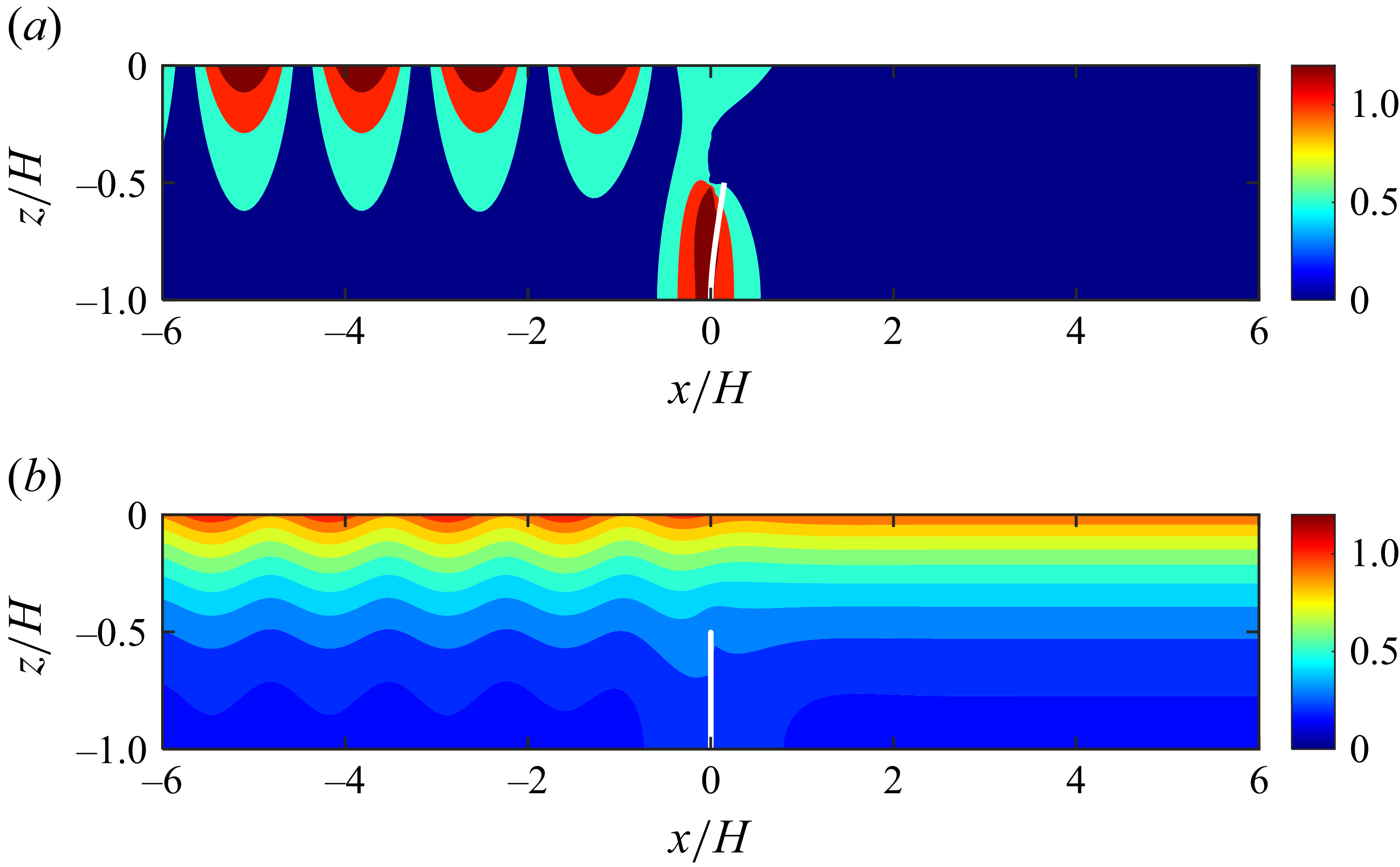
To further visualise the LR effect, the spatial distributions of the normalised velocity potential amplitude $|\phi / \phi ^I(0,0)|$ for both flexible and rigid cases are compared in figure 4. At the resonance frequency, the flexible plate induces a significant local energy amplification (near-field enhancement), as seen in figure 4(a). This energy entrapment is indicative of a strong coupling between the incident wave and the resonant mode, effectively creating a ’soft’ boundary that thwarts wave transmission. Conversely, the potential field around the rigid plate (figure 4 b) exhibits no such localisation, with the wave energy bypassing the structure unhindered. This contrast highlights that the flexible resonator acts as a localised energy sink/reflector, demonstrating its efficacy in wave attenuation.

Figure 4.

Normalised velocity potential fields at resonance ( $\omega =4.85$ rad s⁻¹, $kH = 2.45$ ). (a) Flexible resonator exhibiting local energy amplification. (b) Fixed rigid plate showing unimpeded propagation.

The physical mechanism underlying this wave suppression is rooted in the destructive interference between different wave components. As per (2.25), the total field is a superposition of the incident wave $\eta ^I$ , the diffraction wave $\eta ^D$ from the stationary structure, and the radiation wave $\eta ^R$ induced by the plate’s oscillation. We define the baseline scattered field as $\eta ^S = \eta ^I + \eta ^D$ . Figures 5(a) and 5 (b) compare the amplitude and phase of $\eta ^S$ and $\eta ^R$ . It is observed that while $\eta ^S$ closely mirrors the incident wave, the radiation wave $\eta ^R$ attains a comparable amplitude but maintains an antagonistic phase relationship near resonance.

The amplitude and phase differences are explicitly plotted in figure 5(c). Crucially, at resonance, the radiation wave is exactly $180^\circ$ out of phase with the baseline field ( $\theta (\eta _R-\eta _S) = \pi$ ), leading to a complete phase cancellation in the transmission direction. This antiphase synchrony is a hallmark of LR-based metamaterials. The structural response in figure 5(d) further confirms that the resonator’s motion is consistently in the quadrature-to-antiphase regime ( $[\pi /2, \pi ]$ ) relative to the excitation. Consequently, the energy is redirected upstream (reflection) rather than transmitted, as the group velocity vanishes in the vicinity of this resonant turning point.

Figure 5.

Mechanistic analysis of phase cancellation. (a) Amplitudes and (b) phases of the radiation ( $\eta ^R$ ) and baseline scattered ( $\eta ^S$ ) waves. (c) Amplitude difference and phase difference between $\eta ^R$ and $\eta ^S$ . (d) Modal response amplitude and phase of the flexible resonator.

It is worth noting that the observed wave inhibition is fundamentally a coherent wave-steering effect rather than a dissipative one. In the current potential flow framework, the energy conservation $R^2 + T^2 = 1$ is strictly maintained, confirming that the transmission minima arise from the phase cancellation between the incident and radiation fields rather than the bulk drag typically associated with flexible aquatic vegetation. This resonance-driven mechanism enables the system to achieve significant wave attenuation within a compact footprint, a regime where drag-based dissipation would be insufficient.

3.2. Bandgap characteristics

Building upon the single-resonator analysis, we now investigate the collective spectral properties of an FPMM array. We consider a finite assembly of $N=8$ resonators, maintaining the constituent parameters consistent with table 1. Here, the lattice constant is set to $L=H$ to allow both the LR and BR bandgaps to manifest within a comparable frequency regime, which facilitates a clear and direct comparison of their underlying mechanisms and wave attenuation capabilities.

The scattering performance and dispersion topology of the FPMM are illustrated in figure 6. As shown in figure 6(a), a pronounced transmission minimum ( $T \approx 0$ ) emerges within the interval $2.02 \lt kH \lt 2.45$ . This region is in excellent agreement with the bandgap predicted by the infinite-array dispersion curves (figure 6 c). The emergence of this bandgap is attributed to the coupling of the propagating water wave mode and the localised resonant mode of the flexible plates, leading to a zero-group-velocity regime (Ma & Sheng Reference Ma and Sheng2016). Significantly, the upper bound of this bandgap coincides with the intrinsic resonance frequency of an isolated resonator, confirming its classification as an LR bandgap. The transition from the single-plate response (figure 3 a) to the array response (figure 6 a) highlights the synergistic effect of periodic resonators, which respond collectively to the incident field to suppress wave transmission across a finite frequency band.

To distinguish the LR mechanism from conventional interference effects, the scattering coefficients for a rigid plate array are presented in figure 6(b). A distinct reflection peak is observed around $kH \approx 3$ , governed by the BR condition. This occurs when the scattered waves from periodic heterogeneities interfere constructively, typically when the wavelength $\lambda$ satisfies $2L/\lambda \approx 1$ (Mei Reference Mei1985; Bragg & Bragg Reference Bragg and Bragg1997). The inset in figure 6(b) confirms that the reflection maximum aligns with the Bragg criterion. For the FPMM array, figure 6(c) reveals a dual-bandgap structure: a low-frequency LR bandgap and a higher-frequency BR bandgap. Notably, the BR bandgap in the FPMM case (figure 6 c) shift to higher frequencies compared to the rigid case (figure 6 d). This deviation stems from the hydrodynamic radiation and mutual coupling between the oscillating plates, which modify the effective periodicity of the system. Crucially, the LR bandgap is not only lower in frequency but also significantly broader than the BR bandgap, demonstrating the superior capacity of FPMMs for low-frequency wave control.

Figure 6.

Wave scattering coefficients for $N=8$ periodic cells: (a) flexible plates (FPMM) and (b) rigid plates. The inset in (b) depicts the coefficients versus the dimensionless wavelength $2L/\lambda$ . Dispersion relations for infinite periodic arrays: (c) FPMM and (d) rigid plates.

The spatial evolution of the wave field within the LR bandgap is further examined in figure 7. At a representative frequency ( $kH=2.1$ ), the instantaneous wave profiles (figure 7 a) demonstrate that the radiation field $\eta ^R$ and the baseline scattered field $\eta ^S$ maintain a precise antiphase relationship. This destructive interference is the fundamental mechanism for the vanishing transmission observed in the array. Snapshots of the free-surface elevation and plate deformations at various time intervals (figure 7 b) reveal a rapid spatial decay of the wave amplitude along the array. The upstream resonators intercept the majority of the wave energy, undergoing significant hydroelastic deformation, while the downstream resonators remain nearly quiescent. This effect is further corroborated by the velocity potential distribution in figure 7(c), where the localised energy concentration at the first resonator confirms that wave propagation is effectively halted before penetrating the bulk of the metamaterial.

Figure 7.

(a) Instantaneous wave profiles of the scattering and radiation components at $kH=2.1$ . (b) Temporal evolution of the wave elevation and plate response within one wave period. (c) Normalised velocity potential amplitude $|\phi /\phi ^I(0,0)|$ , illustrating spatial attenuation.

Figure 8.

Evolution of the LR bandgap as a function of (a) the Young’s modulus $E$ , and (b) the plate length $l$ . Other parameters are as specified in table 1.

Finally, we perform a parametric sensitivity analysis to assess the tunability of the LR bandgap. Figure 8(a) shows that increasing the elastic modulus $E$ shifts the bandgap to higher frequencies, as the enhanced structural stiffness elevates the natural frequency of the resonators. Conversely, by reducing the modulus, the bandgap can be tuned towards the low-frequency regime. However, a common bottleneck in traditional acoustic metamaterials is that the bandgap bandwidth typically narrows as the central frequency decreases (Wang et al. Reference Wang, Casadei, Shan, Weaver and Bertoldi2014). As shown in figure 8(b), the FPMM exhibits a remarkable departure from this trend. While increasing the plate length $l$ lowers the resonance frequency due to reduced stiffness, the bandgap width remains surprisingly robust. This phenomenon is rooted in the frequency-dependent nature of the fluid–structure interaction: as the plate size increases, the submerged surface area and the associated hydrodynamic added mass also increase. This compensatory mechanism sustains a strong hydroelastic coupling even at lower frequencies, allowing the FPMM to achieve a robust broadband attenuation performance.

Figure 9.

(a) Schematic of the experimental facility, instrumentation and physical model. Photographs show the experimental arrangement for (b) the flexible plate array and (c) the rigid plate array.

4.1. Experimental set-up

The experimental facility and the configuration of the physical model are illustrated in figure 9(a). The tests were conducted in a wave flume at the Port and Navigation Laboratory, Xiamen University of Technology, which measures 35 m in length, 0.7 m in width, and 0.8 m in depth. A piston-type wavemaker was employed at the upstream end to generate monochromatic waves, while a sloped porous beach was installed at the downstream end to minimise wave reflections. The free-surface elevation was recorded by four resistance-type wave gauges with sampling frequency 200 Hz. Three gauges ( $G_1$ , $G_2$ and $G_3$ ) were positioned upstream of the FPMMs to facilitate the separation of incident and reflected wave components, while a single gauge ( $G_4$ ) was located downstream to measure the transmitted wave field.

Table 2.

Experimental parameters for the water waves and the polypropylene plates. The structural properties represent the mean values obtained from material characterisation tests.

Table 2. Long description

The table presents experimental parameters for water waves and polypropylene plates. It has one row and eight columns. The columns are labeled as follows: H (m), A (m), Tw (s), l (m), b (m), ρ (kg m^-3), E (GPa), and L (m). The row contains the following values: 0.5, 0.02, 0.35, 0.4, 0.0048, 912, 1.74, and 0.5. The table provides mean values obtained from material characterization tests.

The FPMMs investigated in this study consist of five periodic unit cells. As shown in figure 9(b), the plates were bottom-mounted with their transverse axes aligned parallel to the wave crests. The plates were fabricated from polypropylene, selected for its appropriate structural compliance. Two distinct plate lengths, $l = 0.35$ and $0.4$ m, were tested, while the width was set to 0.696 m to ensure a small gap with the flume sidewalls, thereby allowing free deformation without frictional interference. Although the nominal thickness was 0.005 m, actual dimensions were subject to manufacturing tolerances. Consequently, the material properties – density $\rho$ , thickness $b$ , and Young’s modulus $E$ – were precisely measured for the specific polypropylene batch used. The averaged experimental parameters for both the fluid and the structure are summarised in table 2. Although polypropylene is viscoelastic, it is modelled as purely elastic with a constant Young’s modulus. In our narrow, low-frequency test regime ( $0.5$ – $1.4$ Hz), the frequency dependence of the modulus is negligible. Additionally, the internal structural damping is orders of magnitude smaller than the highly dominant hydrodynamic damping, rendering viscoelastic effects secondary.

Each flexible plate was inserted into a U-shaped aluminium channel securely anchored to the flume bed (see figure 9 b), ensuring a fully submerged condition. For comparative analysis, a rigid plate array was also tested. These rigid plates were also made of polypropylene, but with increased thickness of 0.01 m and significantly higher flexural rigidity. As depicted in figure 9(c), both the upper and lower edges of the rigid plates were firmly clamped to ensure that they remained immovable and non-deformable during wave action.

The lattice constant was set to $L = 0.5$ m to satisfy the Bragg condition within the target frequency range. The water depth $H$ was maintained at 0.5 m, and the incident wave amplitude $A$ was fixed at 0.02 m. To characterise the frequency response, each configuration was subjected to 21 regular wave conditions, with periods $T_w$ ranging from 0.7 s to 2.0 s. This corresponds to angular frequency range $\omega \in [3.14, 8.98]$ rad s⁻¹ and non-dimensional wavenumbers $kH \in [0.77, 4.11]$ .

4.2. Experimental results

Systematic laboratory tests were performed on periodic arrays of both rigid and flexible plates to evaluate their wave attenuation performance and investigate the influence of plate length. The parameters for the four experimental configurations (cfgs 1–4) are summarised in table 3.

Table 3.

Summary of experimental test cases.

Table 3. Long description

A table summarizing experimental configurations of rigid and flexible plates. The table has four rows and four columns. Column headers are Configuration, cfg. 1, cfg. 2, cfg. 3, and cfg. 4. Row labels are Plate type and Length l (m). Row 1: Configuration, cfg. 1, cfg. 2, cfg. 3, cfg. 4. Row 2: Plate type, Rigid, Rigid, Flexible, Flexible. Row 3: Length l (m), 0.35, 0.4, 0.35, 0.40.

Figure 10 presents the dispersion curves, along with the transmission and reflection coefficients, as functions of the non-dimensional wavenumber $kH$ for cfgs 1 and 3. As depicted in figure 10(a), the periodic rigid plates (cfg. 1) induce a BR bandgap within the range $kH \in [2.76, 3.12]$ under the prescribed geometry. For the finite array of rigid plates, the experimental reflection and transmission coefficients are compared with theoretical predictions in figures 10(b,c), respectively. A high degree of correlation is observed between the theoretical model and the experimental data in figure 10(b). The BR mechanism, characterised by enhanced reflection, is clearly identified and aligns well with the calculated bandgap. In figure 10(c), while the measured transmission coefficient follows the predicted trend, it remains consistently lower than the theoretical values. This discrepancy is attributed to viscous energy dissipation as waves propagate over the submerged obstacles (Cho et al. Reference Cho, Lee and Kim2004), an effect neglected in the idealised potential flow model.

For the flexible plates (cfg. 3), the dispersion analysis in figure 10(d) predicts an LR bandgap at $kH \in [1.52, 2.59]$ and a subsequent BR gap at $kH \in [3.19, 3.48]$ . The measured $R$ and $T$ for the finite flexible array are shown in figures 10(e) and 10(f). A prominent valley in the transmission coefficient is observed, with values approaching zero. The theoretical analysis confirms that this attenuation is driven by the LR mechanism. A secondary, shallower valley corresponding to the BR gap is also evident in the experimental data. However, notable deviations between the potential flow theory and experimental measurements occur within the LR band for the reflection coefficient (figure 10 e). These discrepancies likely arise from nonlinear hydrodynamic effects, such as local wave breaking or vortex shedding at the plate tips, which will be further analysed in § 4.3.

Figure 10.

Dispersion curves for (a) periodic rigid plates and (d) periodic flexible plates ( $l=0.35$ m). Plots of the theoretical and experimental reflection and transmission coefficients for finite arrays (five cells) of (b,c) rigid and (e, f) flexible plates. Data for the rigid plate baseline are adapted from Jin et al. (Reference Jin, Li, Ding, Xie, Zhou and Zhang2026) with permission.

The influence of increased plate length ( $l = 0.4$ m) is illustrated in figure 11. For the rigid plates (cfg. 2), the BR bandgap shifts and widens to $kH \in [2.51, 3.12]$ . Compared to cfg. 1 ( $l=0.35$ m), the increased length enhances wave reflection and further suppresses transmission, a trend consistently captured by both theory and experiment (figures 11 b,c). The maxima in $R$ and minima in $T$ align precisely with the predicted bandgap region. For the periodic flexible plates (cfg. 4), LR and BR bandgaps coexist, as shown in figure 11(a). In comparison with the shorter plates ( $l=0.35$ m), the LR band shifts towards a lower-frequency regime (lower $kH$ ). This shift is physically consistent with the reduced effective stiffness of the longer plates. In figure 11(e), the theoretical reflection coefficient shows favourable agreement with experimental data, except in the resonance-dominated region $1.1 \lt kH \lt 2.0$ . The transmission spectrum exhibits two distinct valleys corresponding to the LR and BR mechanisms. Notably, the experimental transmission coefficients within the LR band are significantly lower than those in the BR band. This confirms the superior wave attenuation capability of the LR mechanism, particularly for low-frequency broadband wave control.

Figure 11.

Experimental and theoretical results for plates with increased length ( $l=0.4$ m). The panels follow the same definitions as in figure 10.

4.3. Energy dissipation

The deviations observed between the theoretical predictions and experimental measurements can be attributed to several physical factors excluded from the linear, inviscid framework. These include flow separation at the sharp edges of the plates, viscous boundary layer effects, wave breaking, and nonlinear interactions between the incident, reflected and radiated wave components (De Vita et al. Reference De Vita, de, M. and Onorato2025). In this subsection, we quantify the experimental energy dissipation and analyse its underlying mechanisms.

To evaluate the energy loss, a dissipation coefficient is defined as

(4.1) \begin{equation} D = 1 - \big(R^2 + T^2\big). \end{equation}

In linear potential flow theory, $D$ is identically zero. Thus any non-zero value of $D$ serves as a metric for the energy extracted from the coherent wave field by dissipative or nonlinear processes.

Figures 12(a) and 12(b) illustrate the dissipation coefficients for rigid and flexible plates of different lengths. A significant amount of energy dissipation is evident in the experimental data. For the shorter rigid plates ( $l=0.35$ m), $D \approx 0.5$ in the low-frequency regime ( $kH \lt 2$ ), whereas for flexible plates, $D$ reaches as high as 0.9. The increased dissipation in flexible plates suggests that the structural motion significantly enhances the conversion of wave energy into turbulence or higher-order harmonics. Notably, dissipation is more pronounced at low frequencies, which may be linked to larger particle excursion and higher horizontal velocities that promote flow separation. In figure 12(b), the overall trends remain consistent with the shorter plates, though the magnitude of $D$ increases with plate length. Furthermore, $D$ reaches a local minimum within the BR bandgap. This occurs because the majority of the incident energy is reflected by the periodic array, leaving only a small fraction to be dissipated via transmission through the structure.

Figure 12.

Energy dissipation coefficients $D$ for incident waves interacting with rigid and flexible plate arrays, for plate lengths (a) $l=0.35$ m, (b) $l=0.4$ m.

Figure 13.

Experimental free-surface elevation and amplitude spectra for cfg. 1 at $T_w=1.9$ s ( $kH=0.82$ ): (a) time series; (b) amplitude spectra derived via fast Fourier transform of five steady-state wave periods.

One primary source of the apparent energy loss is the transfer of energy to higher-order harmonics via nonlinear interactions. Figure 13 presents the free-surface time series and corresponding frequency spectra for cfg. 1 at $T_w = 1.9$ s ( $kH = 0.82$ ). As shown in figure 13(a), the transmitted amplitude at $G_4$ is substantially attenuated compared to the incident wave. While the upstream wave field (gauges $G_1$ – $G_3$ ) remains nearly monochromatic, the downstream signal at $G_4$ exhibits distinct non-sinusoidal features. The spectral analysis in figure 13(b) confirms that while the incident field is dominated by the fundamental frequency, the transmitted field contains measurable second-order harmonic components. This indicates a nonlinear energy cascade resulting from the interaction between the waves and the submerged obstacles. This process, as discussed by Li et al. (Reference Li, Draycott, Adcock, van den and T.2021a ,Reference Li, Zheng, Lin, Adcock, van den and T. b ) in the context of depth transitions, contributes to the observed discrepancy by redirecting energy from the primary wave frequency.

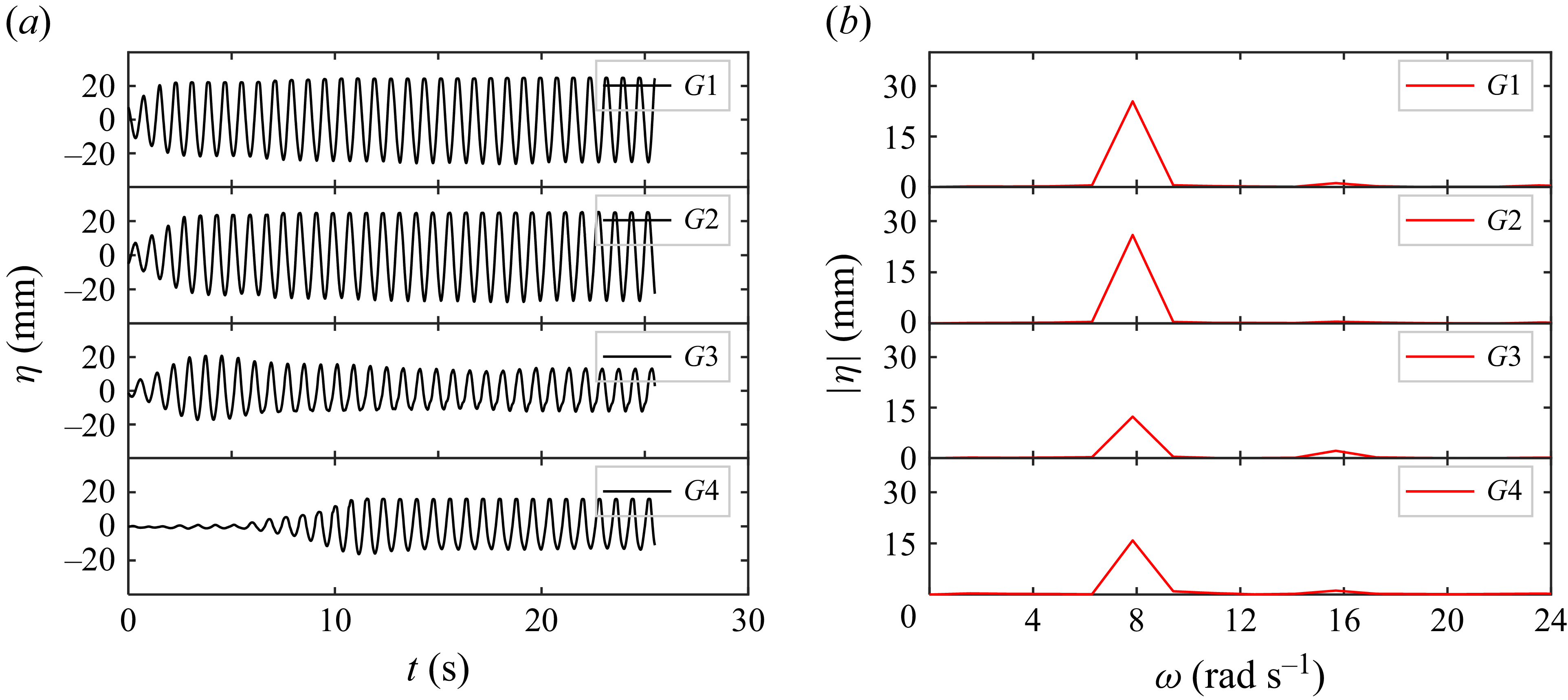
Flow separation at the plate edges also plays a critical role in energy dissipation. Comparison between the low-frequency results in figure 13 and the high-frequency results in figure 14 ( $T_w = 0.8$ s, $kH = 3.19$ ) reveals that the high-frequency waveforms are significantly more stable. According to the dispersion relation, these shorter waves propagate with lower group velocities, which may reduce the intensity of vortex shedding. As noted by Polly et al. (Reference Polly, Mérigaud, Thiria and Godoy-Diana2025), vortices generated at the edges of submerged elastic plates act as significant energy sinks, effectively draining energy from the primary wave mode.

Figure 14.

Experimental free-surface elevation and amplitude spectra for cfg. 1 at a shorter incident wave period $T_w=0.8$ s ( $\omega =7.89\ \text{rad}\ \text{s}^{-1}$ , $kH=3.19$ ): (a) time series; (b) wave amplitude spectra, where five wave periods (12–17 s) from the steady-state portion of the time series were used for fast Fourier transform analysis.

Figure 14. Long description

Panel A: Four line graphs depict time series of free-surface elevation for four different gauges labeled G1, G2, G3, and G4. The horizontal axis represents time in seconds, and the vertical axis represents elevation in millimeters. Each graph shows oscillatory behavior with varying amplitudes and frequencies. Panel B: Four line graphs depict wave amplitude spectra for the same four gauges. The horizontal axis represents angular frequency in radians per second, and the vertical axis represents wave amplitude in millimeters. Each graph shows distinct peaks at specific frequencies, indicating the dominant wave components.

The most prominent factor distinguishing flexible plates from rigid ones is the occurrence of localised wave breaking under resonance conditions. Figure 15 shows the sequential interaction between waves and flexible plates at $T_w = 1.2$ s ( $kH = 1.54$ ). The lead plate undergoes high-amplitude pitch motion. As the plate moves from trough to crest (figures 15 a–d), it acts as a secondary wave source, compressing the fluid and generating radiation waves. Near the equilibrium position (figure 15 c), the plate velocity reaches its maximum, pushing the fluid with sufficient momentum to disrupt the circular orbital motion of the water particles, leading to localised breaking. This breaking process, coupled with the interference between incident and radiation waves, results in a standing-wave-like pattern characterised by severe energy dissipation. This explains why the experimental reflection coefficients for flexible plates are markedly lower than those predicted by potential flow theory.

Figure 15.

Photographs of wave interaction with resonant flexible plates ( $l=0.4$ m, $T_w=1.2$ s, $kH=1.54$ ). Panels (a)–(f) show the sequence at intervals $T_w/6$ .

The supplementary material includes two movies, are available at https://doi.org/10.1017/jfm.2026.11809 comparing the wave response for rigid (cfg. 1) and flexible (cfg. 3) arrays at $T_w = 1.0$ s ( $kH = 2.09$ , the resonant condition for the flexible array). Movie 1 demonstrates that while rigid plates provide some attenuation, significant wave energy still propagates downstream. In contrast, movie 2 shows that the flexible array effectively blocks the incident waves via the LR mechanism. The visible wave breaking in movie 2 further corroborates the role of nonlinear dissipation in the observed experimental results. In essence, the similar dissipation trends observed for rigid and flexible plates at low frequencies are fundamentally driven by incident wave kinematics. However, for the FPMMs, the LR mechanism acts as an amplifier. The localised energy trapping naturally forces the system into a highly dissipative nonlinear regime, significantly intensifying vortex shedding and wave breaking beyond what is achievable by rigid structures.

Although introducing a semi-empirical viscous drag term could force a closer agreement with experimental data, we retain the pure inviscid framework. The observed energy dissipation is driven by complex nonlinear phenomena – primarily localised wave breaking and vortex shedding – that a linearised drag coefficient cannot rigorously represent without ad hoc curve fitting. Preserving the baseline model thus avoids obscuring the underlying physics with empirical tuning.

In summary, the experimental findings confirm the superior wave attenuation capabilities of the LR mechanism in FPMMs. The empirical observation of Bragg reflection in rigid arrays and near-complete attenuation in resonant flexible arrays provides robust support for the proposed metamaterial-based wave control strategy.