


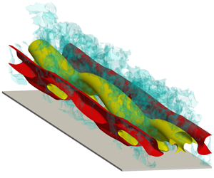


1 Introduction
Solitary waves are long waves of permanent form, which induce approximately constant velocity in the water column (Munk Reference Munk1949). They are subject to friction in the thin boundary layers developing at the free surface and at the sea bottom. The free surface boundary layer is usually weak (Klettner & Eames Reference Klettner and Eames2012), and is negligible. On the other hand, the bottom boundary layer is of prominent importance, as it hosts the hydrodynamic processes driving sediment motion and energy dissipation. In the most basic setting of wave propagating over a smooth bottom in a water of constant depth, the bottom boundary layer consists of regions of favourable and adverse pressure gradients (FPG and APG) located ahead of and behind the wave crest, respectively, cf. figure 1. The boundary layer flow has a tendency to remain laminar in the FPG region. Behind the wave crest, the APG gives rise to an inflectional velocity profile (Liu, Park & Cowen Reference Liu, Park and Cowen2007), cf. velocity profiles in figure 1(a), and the boundary layer becomes linearly unstable (Blondeaux, Pralits & Vittori Reference Blondeaux, Pralits and Vittori2012; Verschaeve & Pedersen Reference Verschaeve and Pedersen2014; Sadek et al. Reference Sadek, Parras, Diamessis and Liu2015). Experimental (Sumer et al. Reference Sumer, Jensen, Sørensen, Fredsøe, Liu and Carstensen2010) and numerical (Vittori & Blondeaux Reference Vittori and Blondeaux2008; Ozdemir, Hsu & Balachandar Reference Ozdemir, Hsu and Balachandar2013) models of the solitary-wave boundary layer (SWBL) have shown that the inflectional instability leads to regularly spaced spanwise-oriented vortex rollers (also known as vortex tubes), which can break down to small-scale turbulence in higher wave amplitudes.
Conceptual sketches showing two main paths of transition to turbulence in the bottom boundary layer under a solitary wave. Scales in the boundary layer are exaggerated for clarity. Laminar velocity profiles are plotted until the onset of transition. (a) Orderly route to transition via two-dimensional modal instabilities initiated by the inflectional velocity profile. (b) Bypass transition initiated by the receptivity of the boundary layer to finite-amplitude ambient disturbances (dashed–dotted curls). The instability is three-dimensional and of a stochastic nature.

Linearly stable base flow in the FPG region does not preclude the onset of transition in this region. Finite amplitude external perturbations such as breaking-wave turbulence, sound or small-scale bedforms can lead to significant growth in finite times and yield secondary base states that can be unstable. Such subcritical transition can take place in the FPG region before the arrival of the wave, and is analogous to bypass transition in zero-pressure gradient (ZPG) boundary layers (Morkovin Reference Morkovin1969), as the modal instability is bypassed by another noise-induced mechanism. This alternative transition scenario is depicted for SWBL in figure 1(b). Unlike the orderly transition, whose initiation is often described simply by a critical Reynolds number, bypass transition is a complicated problem depending on the amplitude, frequency and type of external perturbations in addition to Reynolds number. A recent review on the phenomenology of bypass transition can be found in Durbin (Reference Durbin2017). All bypass scenarios require a receptivity stage, where external perturbations are modified and amplified by the boundary layer, and a breakdown stage, where the most amplified modes become unstable and break into turbulence. The receptivity stage is dominated by streamwise-oriented vortices and streaks. The former are the surviving modes from rapid shear distortion (Phillips Reference Phillips1969) and the latter are elongated streamwise-momentum modes produced by the former via stirring the base flow, a process known as lift-up mechanism (Landahl Reference Landahl1980; Brandt Reference Brandt2014). The initial stages of streak amplification can be linked mathematically to the non-normality of the linearised Navier–Stokes operator (Butler & Farrell Reference Butler and Farrell1992; Trefethen et al. Reference Trefethen, Trefethen, Reddy and Driscoll1993).
The breakdown stage is characterised by secondary instabilities and resultant turbulent spots. Two scenarios have been observed depending on the amplitude of the streaks. When the environment forcing is strong, the lift-up mechanism can generate highly elevated low-speed streaks acting like strong wake perturbations on their environment. These protruding layers are susceptible to wake-like instabilities driven by spanwise shear (Waleffe Reference Waleffe1995; Andersson et al. Reference Andersson, Brandt, Bottaro and Henningson2001; Vaughan & Zaki Reference Vaughan and Zaki2011). Consequently, they develop rapidly growing sinuous undulations, and break down into turbulent spots (Jacobs & Durbin Reference Jacobs and Durbin2001; Matsubara & Alfredsson Reference Matsubara and Alfredsson2001; Hernon, Walsh & McELIGOT Reference Hernon, Walsh and McELIGOT2007). In contrast, when the environment forcing is modest, the streaks are weaker and remain confined to the near-wall region. In this case, instabilities can occur on vertical shear layers that are slightly modulated by streaks. These instabilities are observed to have reduced growth rates compared to reference instabilities (Tollmien–Schlichting (TS) waves), cf. Cossu & Brandt (Reference Cossu and Brandt2004) and Liu, Zaki & Durbin (Reference Liu, Zaki and Durbin2008b). Therefore, introducing moderate-amplitude streaks to the boundary layer can delay the transition point to turbulence (Cossu & Brandt Reference Cossu and Brandt2002). Vaughan & Zaki (Reference Vaughan and Zaki2011) named the two streak instabilities after the location of their respective critical layers and called them ‘outer’ and ‘inner’ modes. We will adapt a similar terminology for the streak instabilities in the present work. The final step of the breakdown stage follows the same path for both inner and outer modes, i.e. turbulent spots at different locations grow and amalgamate (e.g. Narasimha Reference Narasimha1985) and, finally, the turbulent boundary layer sets in.
Unlike flat-plate boundary layers, experimental and numerical evidence for bypass transition in SWBLs are sparse. Using direct numerical simulations (DNS), Ozdemir et al. (Reference Ozdemir, Hsu and Balachandar2013) examined the effect of the perturbation amplitude by seeding white noise of varying magnitudes (between 1–20 % of the maximum free stream velocity) to initial conditions before the arrival of the solitary wave. The cases with 5 % or more noise and  $Re_{\unicode[STIX]{x1D6FF}}\geqslant 1500$, where the Reynolds number is defined using Stokes length and the maximum free stream velocity (cf. § 2 for details), showed an initial energy amplification inside the boundary layer lasting until another more rapidly growing amplification mechanism takes over in the APG stage after flow reversal. They speculated that this early perturbation growth should be due to a nonlinear viscous instability, as it takes place in the FPG stage where velocity profiles do not contain any inflection point, a necessary condition for inviscid instability. However, it is more likely that the amplification is due to linear transient non-normal growth. Indeed, Verschaeve, Pedersen & Tropea (Reference Verschaeve, Pedersen and Tropea2017) found a strong linear non-normal growth in the FPG stage of SWBL if the initial perturbations are organized as streamwise vortices. These vortices then amplify streaks by the lift-up mechanism with a maximum growth proportional to the square of the Reynolds number. Later in the APG stage, the non-normal growth of streaks are overtaken by the non-normal growth of two-dimensional spanwise modes, as the maximum growth of these modes has an exponential scaling in Reynolds number. The analysis of Verschaeve et al. (Reference Verschaeve, Pedersen and Tropea2017) provided conceptual insights for the overtaking of another growth mechanism in the APG stage in Ozdemir et al. (Reference Ozdemir, Hsu and Balachandar2013). However, the critical Reynolds number at which the non-normal two-dimensional modes begin to exert dominance was found to be somewhat different in the DNS study of Ozdemir et al. (Reference Ozdemir, Hsu and Balachandar2013) and in the transient-growth analysis of Verschaeve et al. (Reference Verschaeve, Pedersen and Tropea2017). This is possibly related to nonlinear effects, which are not considered in the study of Verschaeve et al. (Reference Verschaeve, Pedersen and Tropea2017). The transition process in Ozdemir et al. (Reference Ozdemir, Hsu and Balachandar2013) was initiated by regularly spaced spanwise vortex rollers in all cases. Although bypass transition via streak breakdown was not observed, the secondary mechanisms in transition were sensitive to the level of initially seeded perturbation suggesting a sensitivity to the presence of the streaks. Low-noise cases followed a transition path reminiscent of free-shear layers. In contrast, in high-noise cases, where the streaks should be strongest, vortex rollers broke into
 $\unicode[STIX]{x1D6EC}$-shaped vortices, hence, the transition was reminiscent of a K-type transition in flat-plate boundary layers (Klebanoff, Tidstrom & Sargent Reference Klebanoff, Tidstrom and Sargent1962).
Sumer et al. (Reference Sumer, Jensen, Sørensen, Fredsøe, Liu and Carstensen2010) simulated a SWBL in an oscillatory water tunnel and observed turbulent spots in a flow regime starting at  $Re_{\unicode[STIX]{x1D6FF}}=1000$. These sporadic features spread to earlier phases with increasing Reynolds number. At the highest Reynolds number achieved (
 $Re_{\unicode[STIX]{x1D6FF}}=2000$) they could be observed at the end of the FPG stage. Before the nucleation of the spots, the flow remained laminar throughout the FPG stage even at
 $Re_{\unicode[STIX]{x1D6FF}}=2000$. Therefore, Sumer et al. classified the regime
 $Re_{\unicode[STIX]{x1D6FF}}>1000$ as ‘transitional’ and remarked that the upper limit of this regime, in which turbulence spreads over the entire wave event, is unknown, cf. figure 5 in Sumer et al. (Reference Sumer, Jensen, Sørensen, Fredsøe, Liu and Carstensen2010) for details. In some cases, turbulent spots grew until the mid APG stage, and eventually coexisted with the newly developed vortex rollers occupying the laminar regions surrounding them, cf. video 3 in supplemental materials of Sumer et al. (Reference Sumer, Jensen, Sørensen, Fredsøe, Liu and Carstensen2010). The precursor structures to turbulent spots are streamwise streaks, which have also been reported in a prequel paper on oscillatory boundary layers (Carstensen, Sumer & Fredsøe Reference Carstensen, Sumer and Fredsøe2010). It is possible that the same facility-related perturbations excited the flow and produced streaks in both periodic and solitary motions. The characteristics of the ambient noise, e.g. intensity and frequency, were not reported in these experiments. To date, the streak breakdown in SWBLs is explicitly shown only in the DNS study of Sadek (Reference Sadek2015), where a bypass scenario is initiated by seeding optimal streamwise-constant perturbations and some localized secondary perturbations towards the end of the FPG stage. The injected streamwise streaks became unstable and the breakdown to small-scale turbulence took place in the APG stage.
Studies by Ozdemir et al. (Reference Ozdemir, Hsu and Balachandar2013) and Verschaeve et al. (Reference Verschaeve, Pedersen and Tropea2017) imply that the FPG stage of SWBL is receptive to environment perturbations and can respond by developing streaks. There is some experimental evidence that these streaks might breakdown into turbulent spots (Sumer et al. Reference Sumer, Jensen, Sørensen, Fredsøe, Liu and Carstensen2010) or modify the secondary modes of transition when they have modest energy (Ozdemir et al. Reference Ozdemir, Hsu and Balachandar2013). Furthermore, we anticipate that modest-amplitude streaks can have a stabilizing effect on the instabilities developing in the APG stage as in flat-plate boundary layers (Cossu & Brandt Reference Cossu and Brandt2004). There is a need for a systematic study to determine the quantitative and qualitative extent of these effects. In particular, the receptivity and breakdown stages of bypass transition in SWBLs have to be characterised in more detail. The present study is an effort in this direction.
Shoaling waves travel over shallow waters, which can contain turbulence, e.g. in the form of obliquely descending eddies from breaking waves (Nadaoka, Hino & Koyano Reference Nadaoka, Hino and Koyano1989), bottom roughness, e.g. organized as bedforms (Sleath Reference Sleath1984), or sound, e.g. produced by entrained bubbles in the breaking waves (Deane Reference Deane1997). These disturbances in the sea environment continuously force the wave boundary layer in a complicated, unpredictable fashion. To this end, the flow structures dominating the early landscape in the boundary layer are induced by the external perturbations to which the boundary layer shows the strongest response. These perturbations can be identified in an optimization framework using a system perspective, where external disturbances provide the input and the boundary-layer response corresponds to the output. A convenient approach to model the external perturbations is using body forces of a stochastic or deterministic nature. In this context, a deterministic perturbation model allows a more controllable approach, where the frequency and spatial distribution of body forces can be specified. Assuming that perturbations have a small amplitude, a linear approach can be utilized and the response to all possible disturbances in the form of Fourier modes can be investigated. In a pioneering work using this model, Jovanović & Bamieh (Reference Jovanović and Bamieh2005) studied the linear response of the plane Pouseille flow, and identified counter-rotating streamwise-constant vortices as the most ‘dangerous’ perturbation delivering the largest amplification per energy input. The vortices induced energetic streamwise-constant streaks via the lift-up mechanism. This study showed that the linear input-output framework can capture the essence of the receptivity stage despite its simplicity. We will use a similar approach as a starting point in the present analysis and study the receptivity of SWBL. We obtain input-output configurations in the form of streak-vortex systems similar to Jovanović & Bamieh (Reference Jovanović and Bamieh2005). Subsequently, the breakdown stage is investigated with a combination of linear secondary stability analysis and fully nonlinear numerical simulations triggered with finite-amplitude perturbations. We quantify the critical perturbation levels leading to breakdown of streaks via inner and outer secondary instabilities. Interesting results are found implying a dual role for the streaks. Weak to moderate-amplitude streaks and associated inner instabilities are shown to have a stabilizing effect on the boundary layer, whereas higher-amplitude streaks can lead to an early bifurcation to an unstable branch already in the FPG stage.
The manuscript is organized as follows. In § 2 we briefly introduce the SWBL in a temporal setting. Subsequently, the linear input-output framework is described in § 3, where the linear flow response is also discussed. We then select a suitable excitation configuration and embed it to nonlinear governing equations in § 4 to obtain streaky SWBLs, which are the flow response to finite-amplitude excitation. The nonlinear flow response represents the secondary flow states that are amenable to linear instabilities. The character and phase of these instabilities are analysed in § 5 using a linear secondary stability analysis based on a quasi-static assumption. In § 6 the growth and breakdown of streaks is studied using nonlinear DNS. The objective of this section is the validation of quasi-static assumption and the determination of breakdown thresholds. Finally, in § 7 the results are summed up, and implications of the analysis are discussed with some outlook for future work.
2 Problem formulation
We consider a small-amplitude solitary wave with a wave height  $H^{\ast }$ propagating over a constant depth
 $h^{\ast }$. In this work, the physical quantities with an asterisk are dimensional quantities. The problem is defined in a Cartesian coordinate system, where
 $x^{\ast }$ is the direction of wave propagation (also called the streamwise direction),
 $y^{\ast }$ is the spanwise direction parallel to the wave crest and
 $z^{\ast }$ is the vertical direction extending from the bed upwards. The velocity components associated with these directions are
 $u^{\ast }$,
 $v^{\ast }$ and
 $w^{\ast }$, respectively. The surface elevation in the leading order solution is given by (Grimshaw Reference Grimshaw1970)
 $$\begin{eqnarray}\frac{\unicode[STIX]{x1D702}_{w}^{\ast }}{h^{\ast }}=1+\frac{H^{\ast }}{h^{\ast }}\text{sech}^{2}\left(\sqrt{\frac{3H^{\ast }}{4h^{\ast 3}}}(x^{\ast }-c_{w}^{\ast }t^{\ast })\right),\end{eqnarray}$$
where  $c_{w}^{\ast }=\sqrt{g^{\ast }h^{\ast }}$ is the wave speed with
 $g^{\ast }$ being the gravitational acceleration. Furthermore, the irrotational streamwise velocity, which is constant in the water column, is given by
 $$\begin{eqnarray}u_{0}^{\ast }(x^{\ast },t^{\ast })=U_{0m}^{\ast }\text{sech}^{2}\left(\sqrt{\frac{3H^{\ast }}{4h^{\ast 3}}}(x^{\ast }-c_{w}^{\ast }t^{\ast })\right),\end{eqnarray}$$
with the maximum velocity
 $$\begin{eqnarray}U_{0m}^{\ast }=\sqrt{g^{\ast }h^{\ast }}\frac{H^{\ast }}{h^{\ast }}.\end{eqnarray}$$
Adjacent to the bed, there is a bottom boundary layer, in which the streamwise velocity  $u^{\ast }$ has also a rotational velocity component
 $u_{r}^{\ast }$. The thickness of the boundary layer is usually much smaller than the water depth, cf. appendix A in Sumer et al. (Reference Sumer, Jensen, Sørensen, Fredsøe, Liu and Carstensen2010). Therefore, streamwise variations in the boundary layer can be considered negligible compared to temporal and vertical variations. These assumptions allow a local parallel formulation of the bottom boundary layer, where the flow is assumed homogeneous in horizontal directions. At a fixed point, the irrotational velocity at the bottom (free stream velocity hereafter) depends now only on time and reads as
 $$\begin{eqnarray}u_{0}^{\ast }(t^{\ast })=U_{0m}^{\ast }\text{sech}^{2}(-\unicode[STIX]{x1D714}_{w}^{\ast }t^{\ast }),\end{eqnarray}$$
where
 $$\begin{eqnarray}\unicode[STIX]{x1D714}_{w}^{\ast }=\sqrt{\frac{3g^{\ast }H^{\ast }}{4h^{\ast 2}}}\end{eqnarray}$$
is the effective wave frequency. Using the wave frequency and kinematic viscosity, the Stokes length is defined as
 $$\begin{eqnarray}\unicode[STIX]{x1D6FF}_{s}^{\ast }=\sqrt{2\unicode[STIX]{x1D708}^{\ast }/\unicode[STIX]{x1D714}_{w}^{\ast }}\end{eqnarray}$$
as the boundary-layer scale of the problem. Equation (2.4) neglects the first- and higher-order terms in  $H^{\ast }/h^{\ast }$. Therefore, the model is relevant only for
 $H^{\ast }/h^{\ast }\rightarrow 0$. Vittori & Blondeaux (Reference Vittori and Blondeaux2011) employed a less restrictive model, in which first- and second-order terms in
 $H^{\ast }/h^{\ast }$ were also included. The reader is referred to their work for the effect of the wave height on the boundary-layer transition under a solitary wave. Assuming
 $H^{\ast }/h^{\ast }\rightarrow 0$ and
 $\unicode[STIX]{x1D6FF}^{\ast }/h^{\ast }\rightarrow 0$ provides the advantage of reducing the parameter space of the problem to one, the Reynolds number
 $$\begin{eqnarray}Re_{\unicode[STIX]{x1D6FF}}=\frac{U_{0m}^{\ast }\unicode[STIX]{x1D6FF}_{s}^{\ast }}{\unicode[STIX]{x1D708}^{\ast }}.\end{eqnarray}$$
The Stokes length is now the only relevant length scale of the problem.
We introduce the following dimensionless velocity fields, spatial coordinates, time and pressure, respectively,
 $$\begin{eqnarray}\boldsymbol{u}=\boldsymbol{u}^{\ast }/U_{0m}^{\ast },\quad \boldsymbol{x}=\boldsymbol{x}^{\ast }/\unicode[STIX]{x1D6FF}_{s},\quad t=t^{\ast }\unicode[STIX]{x1D714}_{w}^{\ast },\quad p=p^{\ast }/\unicode[STIX]{x1D70C}^{\ast }U_{0m}^{\ast 2}.\end{eqnarray}$$
The momentum equation for the irrotational streamwise velocity at the bottom can be expressed in a local temporal frame approximation as
 $$\begin{eqnarray}\frac{2}{Re_{\unicode[STIX]{x1D6FF}}}\frac{\text{d}u_{0}}{\text{d}t}=-\frac{\unicode[STIX]{x2202}p_{0}}{\unicode[STIX]{x2202}x}.\end{eqnarray}$$
The free stream pressure gradient is calculated using (2.4) and (2.9) and reads as
 $$\begin{eqnarray}-\frac{\unicode[STIX]{x2202}p_{0}}{\unicode[STIX]{x2202}x}=\frac{4}{Re_{\unicode[STIX]{x1D6FF}}}\text{sech}^{2}(-t)\text{tanh}(-t).\end{eqnarray}$$
The non-dimensional pressure gradient and free stream velocity are plotted in figures 2(a) and 2(b), respectively. The overall balance of the streamwise momentum in the laminar SWBL is given by
 $$\begin{eqnarray}\left(\frac{\unicode[STIX]{x2202}}{\unicode[STIX]{x2202}t}-\frac{1}{2}\frac{\unicode[STIX]{x2202}^{2}}{\unicode[STIX]{x2202}z^{2}}\right)U=2\text{sech}^{2}(-t)\text{tanh}(-t),\end{eqnarray}$$
where  $U=u_{r}+u_{0}$ is the total laminar velocity containing both rotational and irrotational components. Equation (2.11) is supplemented with the boundary conditions
 $U(z=0,t)=0$ and
 $U(z\rightarrow \infty ,t)=u_{0}$, and we specify the initial condition
 $U(z,-\infty )=0$. The solution of (2.11) is shown in figure 2(c). This approximate model of SWBL is theoretically solved (Liu & Orfila Reference Liu and Orfila2004) and adapted in experimental (Sumer et al. Reference Sumer, Jensen, Sørensen, Fredsøe, Liu and Carstensen2010; Tanaka et al. Reference Tanaka, Winarta and Yamaji2012) and numerical (Ozdemir et al. Reference Ozdemir, Hsu and Balachandar2013; Sadek et al. Reference Sadek, Parras, Diamessis and Liu2015; Verschaeve et al. Reference Verschaeve, Pedersen and Tropea2017) studies.

3 Optimal disturbances and the flow response
The time-dependent streamwise velocity  $U(z,t)$ in (2.11) is the base state of the problem, which is continuously forced by external perturbations present in the environment. A convenient approach to study the effect of these perturbations is to model them as body forces. In the present parallel flow model, the forcing fields can be defined as the sum of Fourier components
 $$\begin{eqnarray}[f_{u},f_{v},f_{w}](x,y,z,t)=\iiint _{-\infty }^{\infty }[\hat{f}_{u},\hat{f}_{v},\hat{f}_{w}](z)\text{e}^{\text{i}(\unicode[STIX]{x1D6FC}x+\unicode[STIX]{x1D6FD}y+\unicode[STIX]{x1D714}_{f}t)}\,\text{d}\unicode[STIX]{x1D6FC}\,\text{d}\unicode[STIX]{x1D6FD}\,\text{d}\unicode[STIX]{x1D714}_{f},\end{eqnarray}$$
where  $\unicode[STIX]{x1D6FC}$ and
 $\unicode[STIX]{x1D6FD}$ are streamwise and spanwise wavenumbers, respectively, and
 $\unicode[STIX]{x1D714}_{f}$ is the frequency. If we consider small-amplitude perturbations then the flow response to each Fourier component can be studied independently. In this linear regime, the most dangerous flow scenarios can be initiated by finding the Fourier modes inducing the strongest flow response. The objective of this section is to find these Fourier modes using an optimization framework and to analyse the corresponding flow response. In § 3.1 we introduce the optimization problem and the adjoint method to find its solution. Subsequently, the optimal input-output configurations and their scalings are discussed in § 3.2.
3.1 Methodology
We apply a Fourier ansatz in the homogeneous  $x$- and
 $y$-directions for the perturbation velocity and pressure:
 $$\begin{eqnarray}[\tilde{u} ,\tilde{v},\tilde{w},\tilde{p}](x,y,z,t)=\text{Re}\{[\hat{u} ,\hat{v},{\hat{w}},\hat{p}](z,t)\text{e}^{\text{i}(\unicode[STIX]{x1D6FC}x+\unicode[STIX]{x1D6FD}y)}\}.\end{eqnarray}$$
In the linear regime, each Fourier mode is excited by the corresponding harmonic force at the same spatial wavenumber:
 $$\begin{eqnarray}[f_{u},f_{v},f_{w}](x,y,z,t)=\text{Re}\{[\hat{f}_{u},\hat{f}_{v},\hat{f}_{w}](z)\text{e}^{\text{i}(\unicode[STIX]{x1D6FC}x+\unicode[STIX]{x1D6FD}y+\unicode[STIX]{x1D714}_{f}t)}\}.\end{eqnarray}$$
In the present parallel flow model, the perturbation dynamics can be conveniently studied using the forced versions of the Orr–Sommerfeld and Squire (OSS) equations (Schmid & Brandt Reference Schmid and Brandt2014). To this end, two different excitation regimes can be defined. First, when  $t\ll -\unicode[STIX]{x03C0}$, the base flow is vanishingly small, and the forcing brings the stagnant flow to a periodic state, which is given by the set
 $$\begin{eqnarray}\displaystyle & \displaystyle \frac{1}{Re_{\unicode[STIX]{x1D6FF}}}[(2\text{i}\unicode[STIX]{x1D714}_{f}-\hat{\unicode[STIX]{x1D6E5}})\hat{\unicode[STIX]{x1D6E5}}]{\hat{w}}_{o}(z)={\hat{g}}_{w}(z), & \displaystyle\end{eqnarray}$$
 $$\begin{eqnarray}\displaystyle & \displaystyle \frac{1}{Re_{\unicode[STIX]{x1D6FF}}}(2\text{i}\unicode[STIX]{x1D714}_{f}-\hat{\unicode[STIX]{x1D6E5}})\hat{\unicode[STIX]{x1D702}}_{o}(z)={\hat{g}}_{\unicode[STIX]{x1D702}}(z), & \displaystyle\end{eqnarray}$$
 $$\begin{eqnarray}\displaystyle & \displaystyle {\hat{w}}_{o}(0)=\frac{\unicode[STIX]{x2202}{\hat{w}}_{o}}{\unicode[STIX]{x2202}z}(0)=\hat{\unicode[STIX]{x1D702}}_{o}(0)=0, & \displaystyle\end{eqnarray}$$
 $$\begin{eqnarray}\displaystyle & \displaystyle {\hat{w}}_{o}(z\rightarrow \infty )=\frac{\unicode[STIX]{x2202}{\hat{w}}_{o}}{\unicode[STIX]{x2202}z}(z\rightarrow \infty )=\hat{\unicode[STIX]{x1D702}}_{o}(z\rightarrow \infty )=0, & \displaystyle\end{eqnarray}$$
where  ${\hat{w}}_{o}$ and
 $\hat{\unicode[STIX]{x1D702}}_{o}$ are the vertical velocity and vertical vorticity modes associated with the wavenumber pair (
 $\unicode[STIX]{x1D6FC},\unicode[STIX]{x1D6FD}$),
 $\hat{\unicode[STIX]{x1D6E5}}=\unicode[STIX]{x2202}^{2}/\unicode[STIX]{x2202}z^{2}-k^{2}$ represents the semi-discretized Laplacian operator,
 $k^{2}=\unicode[STIX]{x1D6FC}^{2}+\unicode[STIX]{x1D6FD}^{2}$, and
 ${\hat{g}}_{w}$ and
 ${\hat{g}}_{\unicode[STIX]{x1D702}}$ are the external driving forces containing the control variables
 $\hat{\boldsymbol{f}}=(\,\hat{f}_{u},\hat{f}_{v},\hat{f}_{w})$,
 $$\begin{eqnarray}\displaystyle & \displaystyle {\hat{g}}_{w}=-\text{i}\unicode[STIX]{x1D6FC}\frac{\unicode[STIX]{x2202}\hat{f}_{u}}{\unicode[STIX]{x2202}z}-\text{i}\unicode[STIX]{x1D6FD}\frac{\unicode[STIX]{x2202}\hat{f}_{v}}{\unicode[STIX]{x2202}z}-k^{2}\hat{f}_{w}, & \displaystyle\end{eqnarray}$$
 $$\begin{eqnarray}\displaystyle & \displaystyle {\hat{g}}_{\unicode[STIX]{x1D702}}=\text{i}\unicode[STIX]{x1D6FD}\hat{f}_{u}-\text{i}\unicode[STIX]{x1D6FC}\hat{f}_{v}. & \displaystyle\end{eqnarray}$$
When the wave arrives, the flow is no longer periodic, and the perturbation equations become
 $$\begin{eqnarray}\displaystyle & \displaystyle \left[\left(\frac{2}{Re_{\unicode[STIX]{x1D6FF}}}\frac{\unicode[STIX]{x2202}}{\unicode[STIX]{x2202}t}+\text{i}\unicode[STIX]{x1D6FC}U-\frac{1}{Re_{\unicode[STIX]{x1D6FF}}}\hat{\unicode[STIX]{x1D6E5}}\right)\hat{\unicode[STIX]{x1D6E5}}-\text{i}\unicode[STIX]{x1D6FC}\frac{\unicode[STIX]{x2202}^{2}U}{\unicode[STIX]{x2202}z^{2}}\right]{\hat{w}}(z,t)={\hat{g}}_{w}(z)\text{e}^{\text{i}\unicode[STIX]{x1D714}_{f}t}, & \displaystyle\end{eqnarray}$$
 $$\begin{eqnarray}\displaystyle & \displaystyle \left(\frac{2}{Re_{\unicode[STIX]{x1D6FF}}}\frac{\unicode[STIX]{x2202}}{\unicode[STIX]{x2202}t}+\text{i}\unicode[STIX]{x1D6FC}U-\frac{1}{Re_{\unicode[STIX]{x1D6FF}}}\hat{\unicode[STIX]{x1D6E5}}\right)\hat{\unicode[STIX]{x1D702}}(z,t)+\text{i}\unicode[STIX]{x1D6FD}\frac{\unicode[STIX]{x2202}U}{\unicode[STIX]{x2202}z}{\hat{w}}(z,t)={\hat{g}}_{\unicode[STIX]{x1D702}}(z)\text{e}^{\text{i}\unicode[STIX]{x1D714}_{f}t}, & \displaystyle\end{eqnarray}$$
 $$\begin{eqnarray}\displaystyle & \displaystyle {\hat{w}}(z,-\infty )={\hat{w}}_{o}(z);\quad \hat{\unicode[STIX]{x1D702}}(z,-\infty )=\hat{\unicode[STIX]{x1D702}}_{o}(z), & \displaystyle\end{eqnarray}$$
 $$\begin{eqnarray}\displaystyle & \displaystyle {\hat{w}}(0,t)=\frac{\unicode[STIX]{x2202}{\hat{w}}}{\unicode[STIX]{x2202}z}(0,t)=\hat{\unicode[STIX]{x1D702}}(0,t)=0, & \displaystyle\end{eqnarray}$$
 $$\begin{eqnarray}\displaystyle & \displaystyle {\hat{w}}(z\rightarrow \infty ,t)=\frac{\unicode[STIX]{x2202}{\hat{w}}}{\unicode[STIX]{x2202}z}(z\rightarrow \infty ,t)=\hat{\unicode[STIX]{x1D702}}(z\rightarrow \infty ,t)=0, & \displaystyle\end{eqnarray}$$
where  ${\hat{w}}$ and
 $\hat{\unicode[STIX]{x1D702}}$ are the vertical velocity and vorticity modes during the wave event. The following compact notation is used for the periodic and temporal OSS system of equations
 $$\begin{eqnarray}L_{o}\hat{\boldsymbol{q}_{o}}=C\hat{\boldsymbol{f}},\quad L(t)\hat{\boldsymbol{q}}=C\hat{\boldsymbol{f}}\text{e}^{\text{i}\unicode[STIX]{x1D714}_{f}t},\end{eqnarray}$$
where  $\hat{\boldsymbol{q}}_{o}=[{\hat{w}}_{o},\hat{\unicode[STIX]{x1D702}}_{o}]$ and
 $\hat{\boldsymbol{q}}=[{\hat{w}},\hat{\unicode[STIX]{x1D702}}]$.
The response of the flow to an excitation at a wavenumber pair  $(\unicode[STIX]{x1D6FC},\unicode[STIX]{x1D6FD})$ is measured by the perturbation kinetic energy
 $$\begin{eqnarray}E(\hat{\boldsymbol{u}}):={\textstyle \frac{1}{2}}\int _{0}^{\infty }(|\hat{u} |^{2}+|\hat{v}|^{2}+|{\hat{w}}|^{2})\,\text{d}z.\end{eqnarray}$$
We can express  $\hat{u}$ and
 $\hat{v}$ in terms of
 ${\hat{w}}$ and
 $\hat{\unicode[STIX]{x1D702}}$, and obtain (Schmid & Henningson Reference Schmid and Henningson2001)
 $$\begin{eqnarray}\displaystyle E(\hat{\boldsymbol{q}}):=\frac{1}{2k^{2}}\int _{0}^{\infty }(k^{2}|{\hat{w}}|^{2}+\left|\frac{\unicode[STIX]{x2202}{\hat{w}}}{\unicode[STIX]{x2202}z}\right|^{2}+|\hat{\unicode[STIX]{x1D702}}|^{2})\,\text{d}z. & & \displaystyle\end{eqnarray}$$
We look for the most dangerous perturbations initiating the strongest response in the linear SWBL. This is equivalent to finding an optimal control  $\hat{\boldsymbol{f}}^{opt}(z;\unicode[STIX]{x1D6FC},\unicode[STIX]{x1D6FD},\unicode[STIX]{x1D714}_{f},T_{f},Re_{\unicode[STIX]{x1D6FF}})$, which yields the maximum energy amplification at a terminal time
 $t=T_{f}$ per initial energy input
 $E(\hat{\boldsymbol{q}_{o}})$. This is found by solving the constrained optimization problem
 $$\begin{eqnarray}\displaystyle \left.\begin{array}{@{}c@{}}\displaystyle G_{f}(\unicode[STIX]{x1D6FC},\unicode[STIX]{x1D6FD},\unicode[STIX]{x1D714}_{f},T_{f},Re_{\unicode[STIX]{x1D6FF}}):=\max _{\hat{\boldsymbol{f}}}\frac{E(\hat{\boldsymbol{q}}(T_{f}))}{E(\hat{\boldsymbol{q}_{o}})}\\[5.0pt] \displaystyle \text{subject to}\\[5.0pt] \displaystyle L_{o}\hat{\boldsymbol{q}}_{o}=C\hat{\boldsymbol{f}},\\[5.0pt] \displaystyle L(t)\hat{\boldsymbol{q}}=C\hat{\boldsymbol{f}}\text{e}^{\text{i}\unicode[STIX]{x1D714}_{f}t},\\[5.0pt] \displaystyle \Vert \hat{\boldsymbol{f}}\Vert =1,\end{array}\right\} & & \displaystyle\end{eqnarray}$$
where  $G_{f}$ is the largest response or gain. The optimization problem (3.18) is subject to constraints in the form of periodic and transient OSS systems, and to an additional normalization constraint, which ensures the forcing energy is unity. This optimal control analysis is closely related to the optimal transient-growth analysis of Verschaeve et al. (Reference Verschaeve, Pedersen and Tropea2017) but differs in control variables, i.e. instead of the growth of initial perturbations, the response to external forcing is measured.
The optimization problem (3.18) is solved using an adjoint approach (Luchini & Bottaro Reference Luchini and Bottaro2014). In this method, a Lagrangian functional is assigned to the optimization problem, and the optimality conditions are derived from the stationary point of the Lagrangian, cf. appendix A for details. To this end, the gain  $G_{f}$ is maximum when the flow is forced by the optimal forcing configuration
 $\hat{\boldsymbol{f}}^{opt}$ satisfying
 $$\begin{eqnarray}\displaystyle L_{o}\hat{\boldsymbol{q}}_{o} & = & \displaystyle C\hat{\boldsymbol{f}}^{opt},\nonumber\\ \displaystyle L(t)\hat{\boldsymbol{q}} & = & \displaystyle C\hat{\boldsymbol{f}}^{opt}\text{e}^{\text{i}\unicode[STIX]{x1D714}_{f}t},\nonumber\\ \displaystyle L^{+}(t)\hat{\boldsymbol{q}}^{+} & = & \displaystyle 0,\end{eqnarray}$$
 $$\begin{eqnarray}\displaystyle \Vert \,\hat{\boldsymbol{f}}^{opt}\Vert & = & \displaystyle 1,\nonumber\\ \displaystyle \hat{\boldsymbol{f}}^{opt} & = & \displaystyle \unicode[STIX]{x1D711}(\hat{\boldsymbol{q}}^{+}).\end{eqnarray}$$
Equation (3.19) represents the following adjoint Orr–Sommerfeld and Squire equations:
 $$\begin{eqnarray}\displaystyle & \displaystyle \left[\left(\frac{2}{Re_{\unicode[STIX]{x1D6FF}}}\frac{\unicode[STIX]{x2202}}{\unicode[STIX]{x2202}t}+\text{i}\unicode[STIX]{x1D6FC}U+\frac{1}{Re_{\unicode[STIX]{x1D6FF}}}\hat{\unicode[STIX]{x1D6E5}}\right)\hat{\unicode[STIX]{x1D6E5}}+2\text{i}\unicode[STIX]{x1D6FC}\frac{\unicode[STIX]{x2202}U}{\unicode[STIX]{x2202}z}\frac{\unicode[STIX]{x2202}}{\unicode[STIX]{x2202}z}\right]{\hat{w}}^{+}(z,t)=-\text{i}\unicode[STIX]{x1D6FD}\frac{\unicode[STIX]{x2202}U}{\unicode[STIX]{x2202}z}\hat{\unicode[STIX]{x1D702}}^{+}(z,t), & \displaystyle\end{eqnarray}$$
 $$\begin{eqnarray}\displaystyle & \displaystyle \left(\frac{2}{Re_{\unicode[STIX]{x1D6FF}}}\frac{\unicode[STIX]{x2202}}{\unicode[STIX]{x2202}t}+\text{i}\unicode[STIX]{x1D6FC}+\frac{1}{Re_{\unicode[STIX]{x1D6FF}}}\hat{\unicode[STIX]{x1D6E5}}\right)\hat{\unicode[STIX]{x1D702}}^{+}(z,t)=0, & \displaystyle\end{eqnarray}$$
 $$\begin{eqnarray}\displaystyle & \displaystyle {\hat{w}}^{+}(z,T_{f})=-\frac{1}{2k^{2}}\frac{{\hat{w}}(z,T_{f})}{E(\hat{\boldsymbol{q}}_{o})},\quad \hat{\unicode[STIX]{x1D702}}^{+}(z,T_{f})=\frac{1}{2k^{2}}\frac{\hat{\unicode[STIX]{x1D702}}(z,T_{f})}{E(\hat{\boldsymbol{q}}_{o})}, & \displaystyle\end{eqnarray}$$
 $$\begin{eqnarray}\displaystyle & \displaystyle {\hat{w}}^{+}(0,t)=\frac{\unicode[STIX]{x2202}{\hat{w}}^{+}}{\unicode[STIX]{x2202}z}(0,t)=\hat{\unicode[STIX]{x1D702}}^{+}(0,t)=0, & \displaystyle\end{eqnarray}$$
 $$\begin{eqnarray}\displaystyle & \displaystyle {\hat{w}}^{+}(z\rightarrow \infty ,t)=\frac{\unicode[STIX]{x2202}{\hat{w}}^{+}}{\unicode[STIX]{x2202}z}(z\rightarrow \infty ,t)=\hat{\unicode[STIX]{x1D702}}^{+}(z\rightarrow \infty ,t)=0. & \displaystyle\end{eqnarray}$$
The reader is directed to Schmid & Henningson (Reference Schmid and Henningson2001) for a thorough derivation of equations (3.21) and (3.22). Furthermore, (3.20) corresponds to the expressions to calculate the optimal forcing configuration using the adjoint fields, i.e.
 $$\begin{eqnarray}\displaystyle & \displaystyle \hat{f}_{u}^{opt}(z)=-\frac{1}{2\unicode[STIX]{x1D70E}}\int _{-\infty }^{T_{f}}\left(\text{i}\unicode[STIX]{x1D6FC}\frac{\unicode[STIX]{x2202}{\hat{w}}^{+}}{\unicode[STIX]{x2202}z}+\text{i}\unicode[STIX]{x1D6FD}\hat{\unicode[STIX]{x1D702}}^{+}\right)\text{e}^{-\text{i}\unicode[STIX]{x1D714}_{f}t}\,\text{d}t, & \displaystyle\end{eqnarray}$$
 $$\begin{eqnarray}\displaystyle & \displaystyle \hat{f}_{v}^{opt}(z)=\frac{1}{2\unicode[STIX]{x1D70E}}\int _{-\infty }^{T_{f}}\left(-\text{i}\unicode[STIX]{x1D6FD}\frac{\unicode[STIX]{x2202}{\hat{w}}^{+}}{\unicode[STIX]{x2202}z}+\text{i}\unicode[STIX]{x1D6FC}\hat{\unicode[STIX]{x1D702}}^{+}\right)\text{e}^{-\text{i}\unicode[STIX]{x1D714}_{f}t}\,\text{d}t, & \displaystyle\end{eqnarray}$$
 $$\begin{eqnarray}\displaystyle & \displaystyle \hat{f}_{w}^{opt}(z)=-\frac{1}{2\unicode[STIX]{x1D70E}}\int _{-\infty }^{T_{f}}k^{2}{\hat{w}}^{+}\text{e}^{-\text{i}\unicode[STIX]{x1D714}_{f}t}\,\text{d}t, & \displaystyle\end{eqnarray}$$
where  $\unicode[STIX]{x1D70E}$ is a Lagrange multiplier, cf. appendix A for the details of the derivation of (3.26)–(3.28).
Contours of maximum response  $G_{f}(\unicode[STIX]{x1D6FC},\unicode[STIX]{x1D6FD},\unicode[STIX]{x1D714}_{f}=\unicode[STIX]{x1D714}_{f}^{m},T_{f}=0,Re_{\unicode[STIX]{x1D6FF}}=2000)$, cf. (3.18), with respect to spanwise wavenumbers and terminal phase for optimization, where
 $\unicode[STIX]{x1D714}_{f}^{m}$ is the excitation frequency delivering the maximum gain.

The optimization problem in (3.18) is now transformed to a set of equations with (3.4)–(3.7) and (3.10)–(3.14) being the state or forward equations, (3.21)–(3.25) being the adjoint equations and (3.26)–(3.28) being the design equations. These equations are solved in a sequential fashion using a simple adjoint-looping algorithm (Andersson, Berggren & Henningson Reference Andersson, Berggren and Henningson1999). The algorithm starts with an initial guess of  $\hat{\boldsymbol{f}}^{opt}$ and iterates over the following successive steps: (i) calculation of
 $\hat{\boldsymbol{q}}_{o}$ using (3.4)–(3.7); (ii) forward-in-time integration of the state equations (3.10)–(3.14); (iii) backward-in-time integration of the adjoint equations in (3.21) and (3.25); (iv) updating the control terms with the available adjoint fields using (3.26)–(3.28) and
 $\Vert \hat{\boldsymbol{f}}^{opt}\Vert =1$.
Contours of gain  $G_{f}(\unicode[STIX]{x1D6FC}=0,\unicode[STIX]{x1D6FD},\unicode[STIX]{x1D714}_{f},T_{f},Re_{\unicode[STIX]{x1D6FF}}=2000)$ with respect to spanwise wavenumbers and excitation frequency. (a)
 $T_{f}=-\unicode[STIX]{x03C0}/3$; (b)
 $T_{f}=-\unicode[STIX]{x03C0}/6$; (c)
 $T_{f}=0$; (d)
 $T_{f}=\unicode[STIX]{x03C0}/3$. The coordinate of the peak is also indicated in each figure.

The forward and adjoint equations are discretized in space using a spectral method based on Chebyshev polynomials. In this method, the equations are mapped to the domain  $\unicode[STIX]{x1D709}\in [-1,1]$ and the Gauss–Lobatto collocation technique is utilized to obtain the discrete set of equations. This is implemented using the differentiation matrices developed by Weideman & Reddy (Reference Weideman and Reddy2000). Converged results are obtained for a domain size
 $z\in [0,20]$ and resolution of
 $N_{z}=61$ Chebyshev collocation points in the vertical direction. The initial time to start the simulations is selected to be
 $t_{i}=-10\unicode[STIX]{x03C0}$. At this phase the effect of the wave is negligible. The Crank–Nicolson scheme is employed for time integration. The time step size is
 $\unicode[STIX]{x1D6FF}t=\unicode[STIX]{x03C0}/480$. A sensitivity analysis confirmed that the selected spatial and temporal resolutions are sufficient.
3.2 Linear response of the flow
In this section we study the linear response of the flow to the optimal perturbations at different  $\unicode[STIX]{x1D6FC}$,
 $\unicode[STIX]{x1D6FD}$,
 $\unicode[STIX]{x1D714}_{f}$,
 $T_{f}$ and
 $Re_{\unicode[STIX]{x1D6FF}}$. In figure 3 we show the maximum gain among all excitation frequencies for each wavenumber pair
 $(\unicode[STIX]{x1D6FC},\unicode[STIX]{x1D6FD})$ at a moderate Reynolds number
 $Re_{\unicode[STIX]{x1D6FF}}=2000$. The highest Reynolds number achieved in the oscillating water tunnel of Sumer et al. (Reference Sumer, Jensen, Sørensen, Fredsøe, Liu and Carstensen2010) was
 $Re_{\unicode[STIX]{x1D6FF}}=2000$, where they observed turbulent spots at the end of the FPG stage. In order to study the receptivity of SWBL among the FPG stage, the terminal time is selected to be
 $T_{f}=0$. It is observed in figure 3 that SWBL is very receptive to streamwise-constant (
 $\unicode[STIX]{x1D6FC}=0,\unicode[STIX]{x1D6FD}\neq 0$) excitation in the FPG stage and has a very weak response to two-dimensional
 $\unicode[STIX]{x1D6FC}\neq 0,\unicode[STIX]{x1D6FD}=0$ and oblique
 $\unicode[STIX]{x1D6FC}\neq 0,\unicode[STIX]{x1D6FD}\neq 0$ excitations. These modes, mainly two-dimensional ones, only become dominant in the mid to late APG stage with the flow reversal. Therefore, they do not play a role in an early subcritical bypass transition, and will not be discussed in the remainder of the text.
Figure 4 further demonstrates the response of the flow to streamwise-constant excitation on a  $\unicode[STIX]{x1D6FD}{-}\unicode[STIX]{x1D714}_{f}$ plane at several terminal times (
 $T_{f}=-\unicode[STIX]{x03C0}/3,-\unicode[STIX]{x03C0}/6,0$ and
 $\unicode[STIX]{x03C0}/6$) at
 $Re_{\unicode[STIX]{x1D6FF}}=2000$. We see that with increasing terminal time the frequency band to which the flow is sensitive narrows down. Similarly, there is a shift to lower wavenumbers, which can be linked to the growth of the boundary layer (cf. figure 2c). In general, there is a good flow response in
 $\unicode[STIX]{x1D6FD}\in [1.5,2.5]$ and
 $\unicode[STIX]{x1D714}_{f}\in [0,3]$. In this range, the boundary layer amplifies the external disturbances up to about
 $10^{4}$ times from the start of the wave event until a phase at the start of the APG stage (
 $T_{f}=\unicode[STIX]{x03C0}/6$), cf. figure 4(d).
In order to analyse the scaling of the governing equations with Reynolds number in the case of streamwise-constant excitation, we introduce the transformations
 $$\begin{eqnarray}\overline{\overline{\unicode[STIX]{x1D702}}}=\frac{\hat{\unicode[STIX]{x1D702}}}{Re_{\unicode[STIX]{x1D6FF}}^{2}},\quad \overline{w}=\frac{{\hat{w}}}{Re_{\unicode[STIX]{x1D6FF}}},\end{eqnarray}$$
and substitute to streamwise-constant OSS equations (3.10) and (3.11), where the terms with  $\unicode[STIX]{x1D6FC}$ vanish, i.e.
 $$\begin{eqnarray}\displaystyle & \displaystyle 2\left(\frac{\unicode[STIX]{x2202}}{\unicode[STIX]{x2202}t}-\frac{1}{2}\hat{\unicode[STIX]{x1D6E5}}\right)\hat{\unicode[STIX]{x0394}}\overline{w}=\left(-\text{i}\unicode[STIX]{x1D6FD}\frac{\unicode[STIX]{x2202}\hat{f}_{v}}{\unicode[STIX]{x2202}z}-\unicode[STIX]{x1D6FD}^{2}\hat{f}_{w}\right)\text{e}^{\text{i}\unicode[STIX]{x1D714}_{f}t}, & \displaystyle\end{eqnarray}$$
 $$\begin{eqnarray}\displaystyle & \displaystyle 2\left(\frac{\unicode[STIX]{x2202}}{\unicode[STIX]{x2202}t}-\frac{1}{2}\hat{\unicode[STIX]{x1D6E5}}\right)\overline{\overline{\unicode[STIX]{x1D702}}}=\frac{1}{Re_{\unicode[STIX]{x1D6FF}}}\text{i}\unicode[STIX]{x1D6FD}\hat{f}_{u}\text{e}^{\text{i}\unicode[STIX]{x1D714}_{f}t}-\text{i}\unicode[STIX]{x1D6FD}\frac{\unicode[STIX]{x2202}U}{\unicode[STIX]{x2202}z}\overline{w}. & \displaystyle\end{eqnarray}$$
In the scaled streamwise-constant setting, the velocity components become
 $$\begin{eqnarray}\overline{\overline{u}}=\frac{\text{i}}{\unicode[STIX]{x1D6FD}}\overline{\overline{\unicode[STIX]{x1D702}}},\quad \overline{v}=\frac{\text{i}}{\unicode[STIX]{x1D6FD}}\frac{\unicode[STIX]{x2202}\overline{w}}{\unicode[STIX]{x2202}z}.\end{eqnarray}$$
Therefore, the evolution of cross-stream momentum by the velocity components  $v$ and
 $w$ is embedded into (3.30) and the evolution of streamwise momentum by
 $u$ is linked to (3.31). As shown in (3.30) in the streamwise-constant setting, the cross-stream momentum completely decouples from the streamwise momentum. Thus, the cross-stream perturbations are not influenced by the base flow and the wave has no effect on them. The lack of interaction with the wave results in the transverse components remaining in their initial state, i.e.
 $$\begin{eqnarray}\hat{v}=\hat{v}_{o}\text{e}^{\text{i}\unicode[STIX]{x1D714}_{f}t},\quad {\hat{w}}={\hat{w}}_{o}\text{e}^{\text{i}\unicode[STIX]{x1D714}_{f}t}.\end{eqnarray}$$
Therefore, the increase in  $G_{f}$ is solely due to intrinsic amplification of
 $\hat{u}$ by the boundary layer.
Equation (3.30) suggests that introducing  $\overline{w}$ rendered the cross-stream momentum balance independent of the Reynolds number, while (3.31) indicates that the streamwise forcing is one order lower (
 $O(1/Re_{\unicode[STIX]{x1D6FF}})$) than the other
 $O(1)$ terms. Therefore, in high Reynolds numbers, direct streamwise forcing is inefficient, and the optimal external force should concentrate on driving cross-stream components, i.e.
 $$\begin{eqnarray}\Vert \hat{f}_{v}^{opt}\Vert \approx \Vert \hat{f}_{w}^{opt}\Vert \gg \Vert \hat{f}_{u}^{opt}\Vert .\end{eqnarray}$$
Consequently, the streamwise forcing in (3.31) can be neglected for  $Re_{\unicode[STIX]{x1D6FF}}\gg 1$, and the evolution of
 $\overline{\overline{u}}$ becomes independent of Reynolds number. Figure 5 validates these Reynolds-number scalings using the numerical results for the case
 $T_{f}=0,\unicode[STIX]{x1D6FC}=0,\unicode[STIX]{x1D6FD}=1.5$ and
 $\unicode[STIX]{x1D714}_{f}=0$. Similar results are also applicable to other cases. As displayed in figure 5(a) the streamwise component of the optimal force is smaller than the transverse components and it vanishes with increasing Reynolds number. Therefore, the terminal streamwise velocity scaled with
 $Re_{\unicode[STIX]{x1D6FF}}^{2}$ and the terminal vertical velocity scaled with
 $Re_{\unicode[STIX]{x1D6FF}}$ collapse for different Reynolds numbers, cf. figures 5(b) and 5(c).
Reynolds-number dependency of the optimal linear input and output fields. (a) Components of the optimal forcing  $\boldsymbol{f}^{opt}(\unicode[STIX]{x1D6FC}=0,\unicode[STIX]{x1D6FD}=1.5,\unicode[STIX]{x1D714}_{f}=0,T_{f}=0)$ at (⋯):
 $Re_{\unicode[STIX]{x1D6FF}}=125$; (
 $--$):
 $Re_{\unicode[STIX]{x1D6FF}}=500$; (
 $-$):
 $Re_{\unicode[STIX]{x1D6FF}}=2000$. See legends for the colour coding of forcing components. (b) Streamwise velocity
 $|\hat{u} (t=0)|/Re_{\unicode[STIX]{x1D6FF}}^{2}$ at the terminal time
 $t=T_{f}=0$. (c) Vertical velocity
 $|{\hat{w}}_{o}|/Re_{\unicode[STIX]{x1D6FF}}$, which is steady under steady forcing.

Optimal linear input and output configurations in the physical space. (a) Cross-stream components of the optimal steady streamwise-constant force  $\boldsymbol{f}^{opt}(\unicode[STIX]{x1D6FC}=0,\unicode[STIX]{x1D6FD}=1.5,\unicode[STIX]{x1D714}_{f}=0,T_{f}=0,Re_{\unicode[STIX]{x1D6FF}}=2000)$. Filled contours show the forcing magnitude
 $|\boldsymbol{f}^{opt}|/\max \{\boldsymbol{f}^{opt}\}$. Streamwise component is negligible. Arrows show
 $f_{v}^{opt}\hat{\boldsymbol{j}}+f_{w}^{opt}\hat{\boldsymbol{k}}$, where
 $\hat{\boldsymbol{j}}$ are
 $\hat{\boldsymbol{k}}$ are the Cartesian unit vectors in spanwise and vertical directions, respectively. This is the forcing configuration employed for the analysis in §§ 4–6. (b) The flow response at the terminal time
 $t=T_{f}=0$. Filled contours show levels of the streamwise component
 $\tilde{u} /Re_{\unicode[STIX]{x1D6FF}}^{2}$ and line contours show the steady streamfunction
 $\tilde{\unicode[STIX]{x1D713}}_{o}/Re_{\unicode[STIX]{x1D6FF}}$ spanning nine levels between minimum and maximum values in the plane.

We now turn to input and output configurations. The optimal steady streamwise-constant forcing configuration  $\boldsymbol{f}^{opt}(\unicode[STIX]{x1D6FC}=0,\unicode[STIX]{x1D6FD}=1.5,\unicode[STIX]{x1D714}_{f}=0,T_{f}=0)$ and the resulting flow response at the terminal time are shown in the physical space in figures 6(a) and 6(b), respectively. In figure 6(b) the contour lines present the streamfunction defined as
 $$\begin{eqnarray}\tilde{v}=-\frac{\unicode[STIX]{x2202}\tilde{\unicode[STIX]{x1D713}}}{\unicode[STIX]{x2202}z},\quad \tilde{w}=\frac{\unicode[STIX]{x2202}\tilde{\unicode[STIX]{x1D713}}}{\unicode[STIX]{x2202}y}.\end{eqnarray}$$
It is observed that the steady forcing is organized as counter-rotating cells  $(0,\hat{f}_{v}^{opt},\hat{f}_{w}^{opt})$, which induce steady counter-rotating vortices
 $(0,\tilde{v}_{o},\tilde{w}_{o})$. The vortices redistribute the streamwise momentum of the base flow, while they lift up the low-momentum fluid and pull down the high momentum fluid. As a result, streaks that are antiphase, with the vertical velocity are produced, i.e. regions of negative
 $\tilde{u}$ and positive
 $\tilde{w}_{o}$, and vice versa, collapse. There is no feedback from streaks to vortices, as long as the streaks remain stable. We will see later that the same observation also applies to nonlinear streamwise-constant equations. Streaks are merely forced by the linear interaction between the base flow and vertical perturbations. We infer from (3.30) that
 $\hat{f}_{v}$,
 $\hat{f}_{w}$ and
 $\overline{w}$ are of the same order in Reynolds number. Therefore, a transverse steady forcing with an amplitude
 $|\hat{f}_{v}|\approx |\hat{f}_{w}|=O(1/Re_{\unicode[STIX]{x1D6FF}}^{2})$ will induce steady vortices of amplitude
 $|\overline{w}|=O(1/Re_{\unicode[STIX]{x1D6FF}}^{2})$. These vortices then interact with the base flow and produce streaks of amplitude
 $|\overline{\overline{\unicode[STIX]{x1D702}}}|=O(1/Re_{\unicode[STIX]{x1D6FF}}^{2})$, as
 $\overline{w}$ and
 $\overline{\overline{\unicode[STIX]{x1D702}}}$ are of the same order in Reynolds number in (3.31). Converting back to physical variables using
 ${\hat{w}}=Re_{\unicode[STIX]{x1D6FF}}\overline{w}$ and
 $\hat{\unicode[STIX]{x1D702}}=Re_{\unicode[STIX]{x1D6FF}}^{2}\overline{\overline{\unicode[STIX]{x1D702}}}$, forcing of amplitude
 $O(1/Re_{\unicode[STIX]{x1D6FF}}^{2})$ will drive steady vortices of amplitude
 $O(1/Re_{\unicode[STIX]{x1D6FF}})$, which in turn induce streaks of amplitude
 $O(1)$. These streaks will grow with increasing rates associated with the outer-velocity time scales. Waleffe (Reference Waleffe1995) derived a similar streak–vortex system, where
 $O(1)$ streaks synthetically forced by the steady vortices of magnitude
 $O(1/Re_{\unicode[STIX]{x1D6FF}})$. These scalings in Reynolds number also apply to the streaks forced by optimal initial perturbations in the form of counter-rotating vortices in steady boundary layers (Gustavsson Reference Gustavsson1991; Schmid & Henningson Reference Schmid and Henningson2001) and in SWBLs (Verschaeve et al. Reference Verschaeve, Pedersen and Tropea2017).
4 Nonlinear streaks
When the perturbations reach appreciable amplitudes, nonlinear effects should be taken into account. We showed in § 3.2 that the cases with  $\unicode[STIX]{x1D6FD}\neq 0$,
 $\unicode[STIX]{x1D6FC}=0$ and
 $\unicode[STIX]{x1D714}_{f}=0$ present a good balance between the optimality and simplicity. Therefore, hereafter the discussion will focus on optimal steady streamwise-constant perturbations, which are arranged as streaks and vortices. In this configuration, the forcing concentrates in cross-stream components and induces vortices that remain steady also in nonlinear regimes due to lack of interaction with the wave. Therefore, the velocity field of the nonlinear vortices is found from steady nonlinear Navier–Stokes and continuity equations
 $$\begin{eqnarray}\displaystyle & \displaystyle -\frac{1}{Re_{\unicode[STIX]{x1D6FF}}}\unicode[STIX]{x0394}\tilde{v}_{o}=-\frac{\unicode[STIX]{x2202}\tilde{p}_{o}}{\unicode[STIX]{x2202}y}+A_{o}\,f_{v}^{opt}-\left(\tilde{v}_{o}\frac{\unicode[STIX]{x2202}\tilde{v}_{o}}{\unicode[STIX]{x2202}y}+\tilde{w}_{o}\frac{\unicode[STIX]{x2202}\tilde{v}_{o}}{\unicode[STIX]{x2202}z}\right), & \displaystyle\end{eqnarray}$$
 $$\begin{eqnarray}\displaystyle & \displaystyle -\frac{1}{Re_{\unicode[STIX]{x1D6FF}}}\unicode[STIX]{x0394}\tilde{w}_{o}=-\frac{\unicode[STIX]{x2202}\tilde{p}_{o}}{\unicode[STIX]{x2202}z}+A_{o}\,f_{w}^{opt}-\left(\tilde{v}_{o}\frac{\unicode[STIX]{x2202}\tilde{w}_{o}}{\unicode[STIX]{x2202}y}+\tilde{w}_{o}\frac{\unicode[STIX]{x2202}\tilde{w}_{o}}{\unicode[STIX]{x2202}z}\right), & \displaystyle\end{eqnarray}$$
 $$\begin{eqnarray}\displaystyle & \displaystyle \frac{\unicode[STIX]{x2202}\tilde{v}_{o}}{\unicode[STIX]{x2202}y}+\frac{\unicode[STIX]{x2202}\tilde{w}_{o}}{\unicode[STIX]{x2202}z}=0, & \displaystyle\end{eqnarray}$$
where  $A_{o}$ is a small forcing magnitude with
 $A_{o}\ll 1$ and
 $\unicode[STIX]{x1D6E5}$ is the Laplacian operator. The steady vortices excite the streaks via intermodal nonlinear interactions and also via linear interaction with the base flow, i.e.
 $$\begin{eqnarray}\displaystyle \frac{2}{Re_{\unicode[STIX]{x1D6FF}}}\left(\frac{\unicode[STIX]{x2202}}{\unicode[STIX]{x2202}t}-\frac{1}{2}\unicode[STIX]{x1D6E5}\right)\tilde{u} =-\!\left(\tilde{v}_{o}\frac{\unicode[STIX]{x2202}\tilde{u} }{\unicode[STIX]{x2202}y}+\tilde{w}_{o}\frac{\unicode[STIX]{x2202}\tilde{u} }{\unicode[STIX]{x2202}z}+\tilde{w}_{o}\frac{\unicode[STIX]{x2202}U}{\unicode[STIX]{x2202}z}\right), & & \displaystyle\end{eqnarray}$$
where the small streamwise forcing  $A_{o}\,f_{u}^{opt}$ is neglected. As the evolution of the cross-stream momentum remains decoupled from the streamwise momentum also in the nonlinear regime, there is no feedback from nonlinear streaks to vortices as long as streaks go through streamwise-constant deformations, which is the case for the stream-constant excitation. More generic perturbations are to be introduced in § 5. Before proceeding with the results for this nonlinear streak–vortex system, we first transform the nonlinear equations to a more convenient form with the aim of reducing the number of parameters in the analysis. To this end, we introduce the variable
 $$\begin{eqnarray}A=A_{o}Re_{\unicode[STIX]{x1D6FF}}^{2},\end{eqnarray}$$
and define the transformations
 $$\begin{eqnarray}\stackrel{{\approx}}{v},\stackrel{{\approx}}{w},\stackrel{{\approx}}{p}=\frac{Re_{\unicode[STIX]{x1D6FF}}}{A}\tilde{v},\quad \frac{Re_{\unicode[STIX]{x1D6FF}}}{A}\tilde{w},\quad \frac{Re_{\unicode[STIX]{x1D6FF}}^{2}}{A}\tilde{p}.\end{eqnarray}$$
Introducing the transformed variables to the vortex equations (4.1)–(4.3),
 $$\begin{eqnarray}\displaystyle & \displaystyle -\unicode[STIX]{x0394}\,\stackrel{{\approx}}{v}_{o}=-\frac{\unicode[STIX]{x2202}\stackrel{{\approx}}{p}_{o}}{\unicode[STIX]{x2202}y}+f_{v}^{opt}-A\left(\stackrel{{\approx}}{v}_{o}\frac{\unicode[STIX]{x2202}\stackrel{{\approx}}{v}_{o}}{\unicode[STIX]{x2202}y}+\stackrel{{\approx}}{w}_{o}\frac{\unicode[STIX]{x2202}\stackrel{{\approx}}{v}_{o}}{\unicode[STIX]{x2202}z}\right), & \displaystyle\end{eqnarray}$$
 $$\begin{eqnarray}\displaystyle & \displaystyle -\unicode[STIX]{x0394}\,\stackrel{{\approx}}{w}_{o}=-\frac{\unicode[STIX]{x2202}\stackrel{{\approx}}{p}_{o}}{\unicode[STIX]{x2202}z}+f_{w}^{opt}-A\left(\stackrel{{\approx}}{v}_{o}\frac{\unicode[STIX]{x2202}\stackrel{{\approx}}{w}_{o}}{\unicode[STIX]{x2202}y}+\stackrel{{\approx}}{w}_{o}\frac{\unicode[STIX]{x2202}\stackrel{{\approx}}{w}_{o}}{\unicode[STIX]{x2202}z}\right), & \displaystyle\end{eqnarray}$$
 $$\begin{eqnarray}\displaystyle & \displaystyle \frac{\unicode[STIX]{x2202}\stackrel{{\approx}}{v}_{o}}{\unicode[STIX]{x2202}y}+\frac{\unicode[STIX]{x2202}\stackrel{{\approx}}{w}_{o}}{\unicode[STIX]{x2202}z}=0, & \displaystyle\end{eqnarray}$$
and to the streak equation (4.4),
 $$\begin{eqnarray}\displaystyle \left(\frac{\unicode[STIX]{x2202}}{\unicode[STIX]{x2202}t}-\frac{1}{2}\unicode[STIX]{x1D6E5}\right)\tilde{u} =-\frac{A}{2}\left(\stackrel{{\approx}}{v}_{o}\frac{\unicode[STIX]{x2202}\tilde{u} }{\unicode[STIX]{x2202}y}+\stackrel{{\approx}}{w}_{o}\frac{\unicode[STIX]{x2202}\tilde{u} }{\unicode[STIX]{x2202}z}+\stackrel{{\approx}}{w}_{o}\frac{\unicode[STIX]{x2202}U}{\unicode[STIX]{x2202}z}\right). & & \displaystyle\end{eqnarray}$$
Transforming the nonlinear governing equations from (4.1)–(4.4) to (4.7)–(4.10) reduces the parameter space of the problem from two,  $Re_{\unicode[STIX]{x1D6FF}}$ and
 $A_{0}$, to one,
 $A$, which can be considered now as the effective amplitude of the excitation. We reiterate that this one-parameter model is only applicable in the range of
 $Re_{\unicode[STIX]{x1D6FF}}\gg 1$, where the optimal forcing configuration
 $\boldsymbol{f}^{opt}$ does not depend on
 $Re_{\unicode[STIX]{x1D6FF}}$ and has a vanishing streamwise component.
The nonlinear governing equations are solved using the open-source CFD library Nektar++ (Cantwell et al. Reference Cantwell, Moxey, Comerford, Bolis, Rocco, Mengaldo, De Grazia, Yakovlev, Lombard and Ekelschot2015). To this end, a high-order spectral element method is employed in a two-dimensional computational domain extending to  $z\in [0,L_{z}=20]$ in the vertical direction, and to
 $y\in [0,Ly=2\unicode[STIX]{x03C0}/\unicode[STIX]{x1D6FD}]$ in the spanwise direction. Periodicity is applied in the
 $y$-direction. The domain is discretized using a structured two-dimensional grid with
 $N_{y}=24$ and
 $N_{z}=36$ elements in the spanwise and vertical directions, respectively. The grid is clustered towards the wall, and the expansion rate of elements in the vertical direction is set to
 $1.1$. Each spectral element is equipped with two-dimensional nodal expansion bases, which are constructed using Lagrange polynomials that are defined on Gauss–Lobatto–Legendre points (Karniadakis & Sherwin Reference Karniadakis and Sherwin2005). A polynomial order of
 $N_{p}=7$ is employed. At the highest considered Reynolds number (
 $Re_{\unicode[STIX]{x1D6FF}}=4000$), the coarsest grid spacings in wall units are
 $l_{y}^{+}=1.54$ in the spanwise direction and
 $l_{z0}^{+}=0.65$ in the vertical direction between the first two grid points from the wall. The details about wall units will be provided in § 6 when DNS configurations are discussed. The governing equations are projected on the polynomial basis using a continuous Galerkin method. The resulting system of differential algebraic equations is discretized in time using an implicit second-order scheme, cf. Vos et al. (Reference Vos, Eskilsson, Bolis, Chun, Kirby and Sherwin2011) for details. Finally, the coupled linear system of equations is segregated using a velocity-correction scheme (Karniadakis, Israeli & Orszag Reference Karniadakis, Israeli and Orszag1991).
(a) Variation of the vortex amplitudes (4.12) with respect to the forcing amplitude A (4.5) in the case of linearly optimal forcing with  $\unicode[STIX]{x1D6FC}=0,\unicode[STIX]{x1D6FD}=1.5,\unicode[STIX]{x1D714}_{f}=0$, and
 $T_{f}=0$. The symbols mark the values at
 $A=15,50$ and
 $100$, for which the evolution of streak amplitudes (4.11) is shown in (b). The spatial distribution corresponding to the forcing with these amplitudes are presented in figure 8. The light horizontal lines in (b) shows two different critical streak amplitudes that are reported in the literature for the emergence of instabilities on steady streaks. (solid line):
 $A_{s}^{c}=0.152$ by Vaughan & Zaki (Reference Vaughan and Zaki2011); (dashed line):
 $A_{s}^{c}=0.26$ by Andersson et al. (Reference Andersson, Brandt, Bottaro and Henningson2001).

To keep the analysis on the evolution, stability and breakdown of nonlinear streaks in a tractable margin, a selection has to be made for a representative spanwise wavenumber  $\unicode[STIX]{x1D6FD}$ and terminal time
 $T_{f}$. To this end,
 $T_{f}=0$ is a good choice to obtain strong amplification during the FPG stage. Furthermore, we see in figure 4(c,d) that the wavenumber
 $\unicode[STIX]{x1D6FD}=1.5$ shows good performance for time horizons corresponding to the strongest amplifications (
 $T_{f}=0,\unicode[STIX]{x03C0}/6$). Therefore, we will merely consider vortical perturbations induced by optimal forcing
 $\boldsymbol{f}^{opt}(\unicode[STIX]{x1D6FC}=0,\unicode[STIX]{x1D6FD}=1.5,\unicode[STIX]{x1D714}_{f}=0,T_{f}=0)$ in the current and upcoming sections. This forcing configuration was shown in figure 6(a) above.
It is convenient to characterize the nonlinear streaks and vortices via simple scalar measures for their amplitudes. Following Andersson et al. (Reference Andersson, Brandt, Bottaro and Henningson2001), the amplitude of streaks is defined as half of the difference between maximum and minimum perturbation velocities, i.e.
 $$\begin{eqnarray}A_{s}(t)={\textstyle \frac{1}{2}}\big(\!\max _{y,z}\{\tilde{u} (y,z,t)\}-\min _{y,z}\{\tilde{u} (y,z,t)\}\big).\end{eqnarray}$$
In the linear regime  $A_{s}$ approaches to the peak of Fourier mode (
 $\hat{u}$). The amplitude of steady vortices can be prescribed conveniently using the maximum vertical velocity, i.e.
 $$\begin{eqnarray}\tilde{w}_{max}=\max _{y,z}\{\tilde{w}_{o}(y,z)\}.\end{eqnarray}$$
In figure 7(a) we show the variation of the vortex magnitudes with respect to the effective forcing amplitude  $A$. The amplitudes are presented in a
 $Re_{\unicode[STIX]{x1D6FF}}$-independent scaling, i.e.
 $\tilde{w}_{max}Re_{\unicode[STIX]{x1D6FF}}=A\,\stackrel{{\approx}}{w}_{max}$. We see that the vortices are in an approximately linear regime for the considered range of forcing amplitudes
 $A$. Figure 7(b) further shows the temporal evolution of normalized streak amplitudes
 $A_{s}/u_{0}(t)$ for the cases
 $A=15,50$ and
 $100$ corresponding to vortex magnitudes
 $\tilde{w}_{max}=2.8/Re_{\unicode[STIX]{x1D6FF}},9.51/Re_{\unicode[STIX]{x1D6FF}}$ and
 $18.78/Re_{\unicode[STIX]{x1D6FF}}$. The streaks initially grow faster than the free stream velocity and
 $A_{s}/u_{0}(t)$ increases until about
 $t=-2$. Subsequently, there is an equilibrium stage until about
 $t=-0.5$, in which streaks and the free stream velocity grow in proportion, hence,
 $A_{s}/u_{0}(t)$ remains approximately constant. Following this phase, the normalized streak amplitudes increase dramatically, as steady vortices keep pumping momentum into streaks, while the free stream velocity stagnates and decelerates. The critical streak amplitudes calculated by Vaughan & Zaki (Reference Vaughan and Zaki2011) (
 $A_{s}^{c}=0.152$) and by Andersson et al. (Reference Andersson, Brandt, Bottaro and Henningson2001) (
 $A_{s}^{c}=0.26$) for the initiation of instabilities on steady streaks are also shown in figure 7(b). The discrepancy between these critical values is due to differences in the shapes of streaks employed in these works. It is observed that the
 $A=15$ case remains below the critical streak amplitudes in the FPG stage and is expected to be stable in this stage. In contrast, cases
 $A=50$ and
 $100$ exceed the critical values already in the FPG stage, hence, can develop early instabilities. These observations will be confirmed in § 6 using secondary stability analysis.
Nonlinear streaks induced by steady streamwise-constant optimal external excitation  $\boldsymbol{f}^{opt}(\unicode[STIX]{x1D6FC}=0,\unicode[STIX]{x1D6FD}=1.5,\unicode[STIX]{x1D714}_{f}=0,T_{f}=0)$ with different amplitudes: (a)
 $A=0$; (b)
 $A=15$ (
 $\tilde{w}_{max}=2.8/Re_{\unicode[STIX]{x1D6FF}}$); (c)
 $A=50$ (
 $\tilde{w}_{max}=9.51/Re_{\unicode[STIX]{x1D6FF}}$); (d)
 $A=100$ (
 $\tilde{w}_{max}=18.78/Re_{\unicode[STIX]{x1D6FF}}$), cf. (4.5). Filled contours show levels of total streamwise velocity scaled with the local phase value of the free stream velocity, i.e.
 $U_{s}/u_{0}(t)$. Each colour bar on top shows the contour levels in the panes below. The thick red contour lines show
 $u=0$. Black line contours show the streamfunction
 $\tilde{\unicode[STIX]{x1D713}}_{o}$ spanning nine levels between minimum and maximum values at the phase.

The streaky fields induced by linearly optimal steady streamwise-constant forcing are two-dimensional and have three components, i.e.
 $$\begin{eqnarray}[U_{s},V_{s},W_{s}](y,z,t):=[U,0,0](z,t)+[\tilde{u} ,0,0](y,z,t)+[0,\tilde{v}_{o},\tilde{w}_{o}](y,z),\end{eqnarray}$$
where the velocity components associated with the streamwise-constant streak–vortex system,  $\tilde{\boldsymbol{u}}=[\tilde{u} ,\tilde{v}_{o},\tilde{w}_{o}]$, added to the standard laminar profile (
 $U$) of the SWBL. The spatial organization of these fields corresponding to cases
 $A=15,50$ and
 $100$ along with the baseline case (
 $A=0$) are shown in figure 8. Filled contours in figure 8 show the streamwise velocity fields scaled with the local free stream velocity at the respective phase,
 $U_{s}/u_{0}(t)$, and line contours show levels of
 $\stackrel{{\approx}}{\unicode[STIX]{x1D713}}_{o}$. Increasing nonlinearity with increasing
 $A$ leads to more uneven streak growth, where low-speed streaks are lifted up to higher fluid layers and narrow down, e.g. compare the figure 8(b–d). These elevated low-momentum regions, low-speed streaks, are bounded by internal shear layers with strong local spanwise and vertical variations.
In the case of steady streamwise-constant excitation, the gain in the nonlinear regime reads as
 $$\begin{eqnarray}G_{f}(t;\unicode[STIX]{x1D6FD},A,Re_{\unicode[STIX]{x1D6FF}},\unicode[STIX]{x1D6FC}=0,\unicode[STIX]{x1D714}_{f}=0)=\frac{E_{{\mathcal{V}}}(t)}{E_{{\mathcal{V}}o}},\end{eqnarray}$$
where
 $$\begin{eqnarray}E_{{\mathcal{V}}}(t)={\textstyle \frac{1}{2}}\int _{0}^{\infty }\int _{0}^{2\unicode[STIX]{x03C0}/\unicode[STIX]{x1D6FD}}[\tilde{u} ^{2}+\tilde{v}_{o}^{2}+\tilde{w}_{o}^{2}]\,\text{d}y\,\text{d}z,\quad E_{{\mathcal{V}}o}={\textstyle \frac{1}{2}}\int _{0}^{\infty }\int _{0}^{2\unicode[STIX]{x03C0}/\unicode[STIX]{x1D6FD}}\left[\tilde{v}_{o}^{2}+\tilde{w}_{o}^{2}\right]\,\text{d}y\,\text{d}z\end{eqnarray}$$
are the integrated kinetic energy at time  $t$ and the initial energy, respectively. Although the streak–vortex system given by
 $[\tilde{u} ,\stackrel{{\approx}}{v}_{o},\stackrel{{\approx}}{w}_{o}]$ fields is
 $Re_{\unicode[STIX]{x1D6FF}}$-independent, the actual flow is
 $Re_{\unicode[STIX]{x1D6FF}}$-dependent, as the physical cross-stream components are
 $[\tilde{v}_{o},\tilde{w}_{o}]=A/Re_{\unicode[STIX]{x1D6FF}}[\stackrel{{\approx}}{v},\stackrel{{\approx}}{w}]$. Therefore, similarity with respect to
 $A$ only applies to streaks not to vortices, hence the dependency of
 $G_{f}$ on the Reynolds number. We note that
 $\tilde{v}_{o}^{2}$ and
 $\tilde{w}_{o}^{2}$ are two orders lower in Reynolds number than
 $\tilde{u} ^{2}$ and, therefore, can be neglected in sufficiently high Reynolds numbers, i.e.
 $E_{{\mathcal{V}},u}\approx E_{{\mathcal{V}}}$, where
 $E_{{\mathcal{V}},u}$ is the integrated streamwise kinetic energy. Consequently, if we define a gain with similarity variables as
 $$\begin{eqnarray}\tilde{G}_{f}(t;\unicode[STIX]{x1D6FD},A,\unicode[STIX]{x1D6FC}=0,\unicode[STIX]{x1D714}_{f}=0)=\frac{E_{{\mathcal{V}},u}(t)}{\tilde{E}_{{\mathcal{V}}o}},\end{eqnarray}$$
where
 $$\begin{eqnarray}\tilde{E}_{{\mathcal{V}}o}={\textstyle \frac{1}{2}}\int _{0}^{\infty }\int _{0}^{2\unicode[STIX]{x03C0}/\unicode[STIX]{x1D6FD}}\left[\stackrel{{\approx}}{v}_{o}^{2}+\stackrel{{\approx}}{w}_{o}^{2}\right]\,\text{d}y\,\text{d}z,\end{eqnarray}$$
then the quadratic dependency of  $G_{f}$ on the Reynolds number can be shown explicitly as
 $$\begin{eqnarray}G_{f}=\left(\frac{Re_{\unicode[STIX]{x1D6FF}}}{A}\right)^{2}\tilde{G}_{f}.\end{eqnarray}$$
In figure 9 we show the gains for  $A=15,50$ and
 $100$ at
 $Re_{\unicode[STIX]{x1D6FF}}=2000$. The nonlinear saturation greatly limits the amplification of streaks in higher amplitudes and, therefore, the gains are much lower. The streaks amplify until about
 $t\approx 0.9$ and then decay with the flow reversal.


5 Secondary instability of the nonlinear streaks
The modulated SWBL featuring the streaks presents a new laminar state, which can be analysed for its linear stability. In zero-pressure-gradient boundary layers, once the nonlinearity saturates the streaks, their evolution downstream is slow. Therefore, the streamwise velocity on a downstream cross-section is assumed steady and streamwise-invariant, and employed as the base state in the secondary stability analysis (Andersson et al. Reference Andersson, Brandt, Bottaro and Henningson2001). We examine the stability of nonlinear streaks in SWBL using a similar approach. The main challenge in adapting a secondary stability analysis to the present problem is the transient nature of SWBL – streaky base states evolve strongly under the effect of strong dynamic and aperiodic pressure gradients. In this regard, a suitable approach, to identify temporally unstable regions beneath the wave, is the quasi-static stability analysis, in which each instantaneous state is analysed separately for momentary instabilities (Chen & Kirchner Reference Chen and Kirchner1971). Such an assumption is only valid if the growth rate of the instability is significantly higher than that of the mean flow. In this regard, the quasi-static assumption is not ideal to draw instability balloons of a transient flow, as close to critical conditions the growth rates become too small to satisfy the quasi-static assumption (Von Kerczek & Davis Reference Von Kerczek and Davis1974). Nevertheless, the approach is quite useful to identify rapidly growing instabilities relevant for transition to turbulence in the SWBL. The quasi-static assumption for the present flow will be validated in § 6 using DNS.
Blondeaux et al. (Reference Blondeaux, Pralits and Vittori2012) applied the quasi-static stability analysis to SWBL by considering two-dimensional perturbations growing on one-dimensional, one-component base profiles  $U(z,t)$. Here, the analysis is extended to two-dimensional streaky fields with three components
 $[U_{s},V_{s},W_{s}](y,z,t)$, as shown in (4.13). We consider three-dimensional tertiary perturbations of the form
 $$\begin{eqnarray}[u^{\prime },v^{\prime },w^{\prime },p^{\prime }](x,y,z,t)=\text{Re}\{[\hat{u} ^{\prime },\hat{v}^{\prime },{\hat{w}}^{\prime },\hat{p}^{\prime }](y,z,t)\text{e}^{\text{i}(\unicode[STIX]{x1D6FC}x-\int _{0}^{t}\unicode[STIX]{x1D714}(\unicode[STIX]{x1D70F})\,\text{d}\unicode[STIX]{x1D70F})}\},\end{eqnarray}$$
where  $\unicode[STIX]{x1D6FC}$ are real wavenumbers and
 $\unicode[STIX]{x1D714}=\unicode[STIX]{x1D714}_{\text{r}}+\text{i}\unicode[STIX]{x1D714}_{i}$ are associated complex frequencies. Introducing these perturbations to incompressible Navier–Stokes equations, and linearizing the resulting equations around the two-dimensional frozen base state
 $[U_{s},V_{s},W_{s}](y,z,t)$, we obtain
 $$\begin{eqnarray}\displaystyle \hspace{-12.0pt} & \displaystyle -\frac{2}{Re_{\unicode[STIX]{x1D6FF}}}\text{i}\unicode[STIX]{x1D714}\hat{u} ^{\prime }+\text{i}\unicode[STIX]{x1D6FC}U_{s}\hat{u} ^{\prime }+V_{s}\frac{\unicode[STIX]{x2202}\hat{u} ^{\prime }}{\unicode[STIX]{x2202}y}+W_{s}\frac{\unicode[STIX]{x2202}\hat{u} ^{\prime }}{\unicode[STIX]{x2202}z}+\hat{v}^{\prime }\frac{\unicode[STIX]{x2202}U_{s}}{\unicode[STIX]{x2202}y}+{\hat{w}}^{\prime }\frac{\unicode[STIX]{x2202}U_{s}}{\unicode[STIX]{x2202}z}-\frac{1}{Re_{\unicode[STIX]{x1D6FF}}}\unicode[STIX]{x0394}\hat{u} ^{\prime }=-\text{i}\unicode[STIX]{x1D6FC}\hat{p}^{\prime }, & \displaystyle\end{eqnarray}$$
 $$\begin{eqnarray}\displaystyle \hspace{-12.0pt} & \displaystyle -\frac{2}{Re_{\unicode[STIX]{x1D6FF}}}\text{i}\unicode[STIX]{x1D714}\hat{v}^{\prime }+\text{i}\unicode[STIX]{x1D6FC}U_{s}\hat{v}^{\prime }+V_{s}\frac{\unicode[STIX]{x2202}\hat{v}^{\prime }}{\unicode[STIX]{x2202}y}+W_{s}\frac{\unicode[STIX]{x2202}\hat{v}^{\prime }}{\unicode[STIX]{x2202}z}+\hat{v}^{\prime }\frac{\unicode[STIX]{x2202}V_{s}}{\unicode[STIX]{x2202}y}+{\hat{w}}^{\prime }\frac{\unicode[STIX]{x2202}V_{s}}{\unicode[STIX]{x2202}z}-\frac{1}{Re_{\unicode[STIX]{x1D6FF}}}\unicode[STIX]{x0394}\hat{v}^{\prime }=-\frac{\unicode[STIX]{x2202}\hat{p}^{\prime }}{\unicode[STIX]{x2202}y}, & \displaystyle\end{eqnarray}$$
 $$\begin{eqnarray}\displaystyle \hspace{-12.0pt} & \displaystyle -\frac{2}{Re_{\unicode[STIX]{x1D6FF}}}\text{i}\unicode[STIX]{x1D714}{\hat{w}}^{\prime }+\text{i}\unicode[STIX]{x1D6FC}U_{s}{\hat{w}}^{\prime }+V_{s}\frac{\unicode[STIX]{x2202}{\hat{w}}^{\prime }}{\unicode[STIX]{x2202}y}+W_{s}\frac{\unicode[STIX]{x2202}{\hat{w}}^{\prime }}{\unicode[STIX]{x2202}z}+\hat{v}^{\prime }\frac{\unicode[STIX]{x2202}W_{s}}{\unicode[STIX]{x2202}y}+{\hat{w}}^{\prime }\frac{\unicode[STIX]{x2202}W_{s}}{\unicode[STIX]{x2202}z}-\frac{1}{Re_{\unicode[STIX]{x1D6FF}}}\unicode[STIX]{x0394}{\hat{w}}^{\prime }=-\frac{\unicode[STIX]{x2202}\hat{p}^{\prime }}{\unicode[STIX]{x2202}z}, & \displaystyle\end{eqnarray}$$
 $$\begin{eqnarray}\displaystyle \hspace{-12.0pt} & \displaystyle \text{i}\unicode[STIX]{x1D6FC}\hat{u} ^{\prime }+\frac{\unicode[STIX]{x2202}\hat{v}^{\prime }}{\unicode[STIX]{x2202}y}+\frac{\unicode[STIX]{x2202}{\hat{w}}^{\prime }}{\unicode[STIX]{x2202}z}=0. & \displaystyle\end{eqnarray}$$
These equations are complemented with boundary conditions  $\hat{u} ^{\prime }=\hat{v}^{\prime }={\hat{w}}^{\prime }=0$ on
 $z=0$ and
 $z\rightarrow \infty$. The system of equations (5.2)–(5.5) can be written shortly as
 $L^{\prime }(U(t))\hat{\boldsymbol{q}}^{\prime }=\unicode[STIX]{x1D714}(t)\hat{\boldsymbol{q}}^{\prime }$, where
 $\hat{\boldsymbol{q}}^{\prime }(y,z,t)=[\hat{u} ^{\prime },\hat{v}^{\prime },{\hat{w}}^{\prime },\hat{p}^{\prime }](y,z,t)$. Using the quasi-static approximation, an eigenvalue problem is defined by freezing the operator
 $L^{\prime }$ at a temporal station
 $t=t_{s}$ and solving for
 $\unicode[STIX]{x1D714}(t_{s})$ and
 $\hat{\boldsymbol{q}}^{\prime }(y,z,t_{s})$, the eigenvalue and associated eigenfunction at
 $t_{s}$. The solution of the eigenproblem at each phase is obtained with Nektar++ using an Arnoldi algorithm developed by Tuckerman & Barkley (Reference Tuckerman and Barkley2000) and Barkley, Blackburn & Sherwin (Reference Barkley, Blackburn and Sherwin2008). We refer the reader to Rocco (Reference Rocco2014) for the details. For several representative cases, we have cross-checked the calculated leading eigenvalues with the ones obtained by simple power iterations, where the linear equations with random initial conditions are integrated in time until convergence to the leading eigenvalue is achieved. Excellent agreements are found for the imaginary parts of eigenvalues (growth rates), but noticeable differences in real parts (frequencies) are observed. Since real parts obtained with the Arnoldi method appeared to be more sensitive to configuration parameters, we shall use the results from power iterations in the presentation of phase velocities.
Symmetries in the two-dimensional streaky fields allow six different groups of secondary perturbations: sinuous or varicose perturbations associated with fundamental, subharmonic and detuned modes. Sinuous perturbations have a streamwise velocity pattern that is symmetric with respect to the underlying base streak. In contrast, varicose perturbations have antisymmetric streamwise velocity patterns. Fundamental modes share the same spanwise periodicity with the base flow, subharmonic modes have twice the periodicity of the base flow, and detuned modes correspond to the remaining modes, cf. Reddy et al. (Reference Reddy, Schmid, Baggett and Henningson1998) for mathematical details and figure 2 in Andersson et al. (Reference Andersson, Brandt, Bottaro and Henningson2001) for symmetry patterns. In ZPG boundary layers, the most unstable eigenvalues are associated with sinuous perturbations. Using an inviscid analysis, Andersson et al. (Reference Andersson, Brandt, Bottaro and Henningson2001) reported that fundamental and subharmonic sinuous modes have comparable growth rates with subharmonic modes. The eigenfunctions of both fundamental and subharmonic sinuous modes concentrate in regions on the elevated shear layers around low-speed streaks with very similar patterns, but fundamental modes are slightly more localized (figures 12a and 12b in Andersson et al. (Reference Andersson, Brandt, Bottaro and Henningson2001)). Ricco, Luo & Wu (Reference Ricco, Luo and Wu2011) employed a more comprehensive model accounting for the effects of spatial growth and unsteadiness of streaks, and found that fundamental sinuous modes are the most unstable modes. In stochastic bypass-transition scenarios driven by free stream turbulence, the transition is usually initiated by breakdown of a single streak (Hack & Zaki Reference Hack and Zaki2014). Therefore, the fundamental instabilities, with their more localized nature around the base streak, are possibly more representative for practical situations. In this regard, we consider only fundamental-mode instabilities in the present analysis, which allows us to use a periodic domain with a single streak. The spatial discretization on the  $y$–
 $z$ plane is identical with § 4. Only leading eigenvalues and eigenmodes are calculated.
As in § 4, we only consider nonlinear streaks induced by streamwise-constant time-invariant excitation  $f^{opt}(\unicode[STIX]{x1D6FC}=0,\unicode[STIX]{x1D6FD}=1.5,\unicode[STIX]{x1D714}_{f}=0,T_{f}=0,Re_{\unicode[STIX]{x1D6FF}})$. In figure 10(b) we show the maximum leading eigenvalues along all streamwise wavenumbers,
 $\unicode[STIX]{x1D714}_{i}^{max}(t)=\max _{\unicode[STIX]{x1D6FC}}\{\unicode[STIX]{x1D714}_{i}(\unicode[STIX]{x1D6FC},t)\}$ for varying excitation amplitudes
 $A$, (4.5). The stability boundaries are demonstrated with thick contour lines in figure 10(b). A slightly positive value
 $\unicode[STIX]{x1D714}_{i}^{max}/Re_{\unicode[STIX]{x1D6FF}}=0.0001$ is employed, as the exact neutral curve (
 $\unicode[STIX]{x1D714}_{i}^{max}=0$) was quite noisy in early times. It should be stressed that the exact location of the neutral curve has little practical bearing, as the quasi-static assumption is only physically relevant when the instabilities evolve faster than the base flow. For weak perturbations in the range
 $A\lesssim 35$, it is observed that the boundary layer remains stable throughout the FPG stage and becomes unstable only when the APG stage starts, i.e. the crest of the wave passes the probing location. With further increasing forcing amplitude (
 $A>35$), the instabilities also spread to the FPG stage. The growth rates for the stronger streaks in this range rise until the flow reversal in the early APG stage and peak roughly at a phase when maximum streak amplitudes are observed (cf. figure 9).
Stability of the SWBL perturbed by the linearly optimal excitation  $f^{opt}(\unicode[STIX]{x1D6FC}=0,\unicode[STIX]{x1D6FD}=1.5,\unicode[STIX]{x1D714}_{f}=0,T_{f}=0)$. (a) Free stream velocity. (b) Contours of leading imaginary eigenvalues at
 $Re_{\unicode[STIX]{x1D6FF}}=2000$ calculated with separate stability analysis at each
 $(A,t)$ using a quasi-static assumption. The presented values are the maximum values along all streamwise wavenumbers (
 $\unicode[STIX]{x1D6FC}$). Thick contour lines show
 $\unicode[STIX]{x1D714}_{i}/Re_{\unicode[STIX]{x1D6FF}}=0.0001$. (c) The maximum growth rates of the nonlinear streaks forced with
 $A=0,15,50$ and 100 (cf. figure 8). (dotted line):
 $Re_{\unicode[STIX]{x1D6FF}}=650$; (dashed line):
 $Re_{\unicode[STIX]{x1D6FF}}=1000$; (solid line):
 $Re_{\unicode[STIX]{x1D6FF}}=2000$; (dashed–dotted line):
 $Re_{\unicode[STIX]{x1D6FF}}=4000$.

The maximum growth rates calculated at  $Re_{\unicode[STIX]{x1D6FF}}=650,1000,2000$ and 4000 are shown separately in figure 10(c) for cases
 $A=0,15,50$ and 100, for which the streak amplitudes are plotted in figure 7(b) and the base states are presented in figure 8. The results for the unperturbed case
 $A=0$ corresponds to the growth rates of the primary two-dimensional instabilities. These orderly instabilities take place in the APG stage following the emergence of inflectional profiles. The details of the primary instabilities are well documented elsewhere, e.g. Blondeaux et al. (Reference Blondeaux, Pralits and Vittori2012) and Sadek et al. (Reference Sadek, Parras, Diamessis and Liu2015). The
 $A=15$ case represents a case in the regime with weak streak amplitudes (figure 7b). Interestingly, the secondary instability in this case has lower growth rates than the baseline primary instability. In the peaking phase (
 $t\approx 1$), the growth rate in
 $A=15$ is about half of the one in
 $A=0$. These reduced growth rates suggest a damping mechanism introduced to the flow by weak-amplitude streaks. This will be elaborated later. The last two cases,
 $A=50$ and
 $100$, showcase the results for strong streaks that can develop instabilities already in the FPG stage. As the FPG stage is linearly stable in the unperturbed SWBL, these early instabilities in the FPG stage imply a possibility for a subcritical transition. The seeding phase of the instabilities in
 $A=50$ and
 $A=100$ roughly corresponds to the phases when the streak amplitudes exceed the critical threshold given by Vaughan & Zaki (Reference Vaughan and Zaki2011), cf. figure 7(b). We further see in figure 10(c) that instabilities in
 $A=50$ and
 $100$ rapidly converge to the inviscid limit. There is a very good collapse for the scaled growth rates,
 $\unicode[STIX]{x1D714}_{i}^{max}/Re_{\unicode[STIX]{x1D6FF}}$, at Reynolds numbers
 $Re_{\unicode[STIX]{x1D6FF}}=2000,4000$ and the values at the lower Reynolds numbers
 $Re_{\unicode[STIX]{x1D6FF}}=650,1000$ are only slightly smaller. In contrast, there is a stronger dependence on Reynolds number for the cases
 $A=0$ and
 $A=15$, for which we observe a more noticeable difference between scaled growth rates, especially for
 $Re_{\unicode[STIX]{x1D6FF}}=650,1000$. We refer the reader to Sadek (Reference Sadek2015) for the analysis of Reynolds-number dependency of the primary two-dimensional instabilities (
 $A=0$).
It was observed in figure 10 that the streaks have a dual role in the transition to turbulence beneath solitary waves: they can be stabilizing or destabilizing depending on their amplitude. This can be elaborated by considering the overall growth of the perturbation energy in time. Using the ansatz (5.1), the energy at a mode is expressed by
 $$\begin{eqnarray}E_{\unicode[STIX]{x1D6FC}}(t)=E_{0}\text{e}^{2\int _{0}^{t}\unicode[STIX]{x1D714}_{i}(\unicode[STIX]{x1D70F})\,\text{d}\unicode[STIX]{x1D70F}},\end{eqnarray}$$
where  $E_{0}$ is the initial energy density at the mode. In figure 11 we demonstrate the variation of
 $E_{\unicode[STIX]{x1D6FC}}$ at
 $t=\unicode[STIX]{x03C0}$ with respect to
 $A$. In this figure, the most unstable
 $\unicode[STIX]{x1D6FC}$ for each respective
 $A$ is evaluated. Three different instability regimes are observed: (i) primary instability (
 $A=0$); (ii) inner-instability regime (say
 $0<A<20$ or
 $0<\tilde{w}_{max}<3.76/Re_{\unicode[STIX]{x1D6FF}}$ using figure 7a), and (iii) outer-instability regime (
 $A>20$ or
 $\tilde{w}_{max}>3.76/Re_{\unicode[STIX]{x1D6FF}}$). We employed here the naming convention proposed by Vaughan & Zaki (Reference Vaughan and Zaki2011), where ‘inner’ and ‘outer’ refer to the location of the critical layer. In the inner-instability regime, streaks are weak but still effective in mixing the momentum of the base profiles and introducing a damping effect. Consequently, there is a reduction in the growth rates of instabilities. A similar stabilizing effect is observed in flat-plate boundary layers when moderate-amplitude streaks are superposed on TS waves (Cossu & Brandt Reference Cossu and Brandt2004; Liu et al. Reference Liu, Zaki and Durbin2008b). The temporally unstable phases in the inner-instability regime roughly overlaps with the baseline instabilities in the undisturbed regime (cf. figure 10b), which suggests a modified instability of similar nature, where the primary driving mechanism is vertical shear (
 $\unicode[STIX]{x2202}U_{s}/\unicode[STIX]{x2202}z$). We will show later the inner instabilities develop in regions nearer to the wall, where the vertical shear is strong, hence the name ‘inner’. In the third regime, the streaks are strong enough to develop secondary shear layer instabilities in the elevated outer zones. The overall growth due to these instabilities rise dramatically between
 $20<A<60$. Afterwards, there is a saturation range until
 $A\approx 90$, in which increased forcing does not lead to substantial growth. However, with further increasing
 $A$ there is another receptive regime for
 $A>90$.
The overall growth measured by the modal perturbation kinetic energy density  $E_{\unicode[STIX]{x1D6FC}}$ at
 $t=\unicode[STIX]{x03C0}$, cf. (5.6). The initial energy density is set to
 $E_{0}=1$. The most unstable streamwise wavenumber (
 $\unicode[STIX]{x1D6FC}$) is employed at each
 $A$. The symbols refer to the cases
 $A=0,15,50$ and
 $100$, which are further elaborated in figures 12 and 13.

The variation of leading imaginary eigenvalues with respect to streamwise wavenumber for the streaks induced by linearly optimal excitation  $f^{opt}(\unicode[STIX]{x1D6FC}=0,\unicode[STIX]{x1D6FD}=1.5,\unicode[STIX]{x1D714}_{f}=0,T_{f}=0,Re_{\unicode[STIX]{x1D6FF}}=2000)$. (a) Baseline case with
 $A=0$ (4.5) corresponding to the vortex magnitude
 $\tilde{w}_{max}=0$ (4.12); (b)
 $A=15,\tilde{w}_{max}=0.0014$; (c)
 $A=50,\tilde{w}_{max}=0.0048$;(d)
 $A=100,\tilde{w}_{max}=0.0094$. Colour scales of the contours are different in each pane and are shown in separate colour bars next to the panes.

Filled red contours show four different levels of the modulus of the streamwise component of the leading eigenmodes,  $|\hat{u}^{\prime }|$, calculated at four different times
 $t=-\unicode[STIX]{x03C0}/6,0,\unicode[STIX]{x03C0}/6,\unicode[STIX]{x03C0}/3$. The base states are nonlinear streaks induced by the linearly optimal excitation
 $f^{opt}(\unicode[STIX]{x1D6FC}=0,\unicode[STIX]{x1D6FD}=1.5,\unicode[STIX]{x1D714}_{f}=0,T_{f}=0,Re_{\unicode[STIX]{x1D6FF}}=2000)$ for excitation magnitudes (a–d):
 $A=0,\unicode[STIX]{x1D6FC}=0.45$; (e–h):
 $A=15,\unicode[STIX]{x1D6FC}=0.35$; (i–l):
 $A=50,\unicode[STIX]{x1D6FC}=0.75$; (m–p):
 $A=100$,
 $\unicode[STIX]{x1D6FC}=0.75$. Contour lines show the streamwise component of the base flow scaled with the free stream velocity at the respective phase,
 $U_{s}(y,z,\unicode[STIX]{x1D703}_{s}=-40^{\circ })/u_{0}(t)=\{0.1:0.1:0.9\}$. The dashed lines represent the critical velocity level
 $U_{s}^{c}$, at which
 $U_{s}=c_{r}$.

In figure 12 we demonstrate the variation of growth rates with respect to streamwise wavenumbers  $\unicode[STIX]{x1D6FC}$ for cases
 $A=0,15,50$ and
 $100$ calculated at
 $Re_{\unicode[STIX]{x1D6FF}}=2000$. It is observed that the primary instabilities have relatively longer wavelength peaking at wavenumbers around
 $\unicode[STIX]{x1D6FC}\approx 0.45$ (figure 12a), where the outer instabilities concentrate in shorter wavelengths, e.g.
 $\unicode[STIX]{x1D6FC}\approx \unicode[STIX]{x1D6FD}/2\approx 0.75$ for
 $A=50$ (figure 12c) and
 $\unicode[STIX]{x1D6FC}\approx \unicode[STIX]{x1D6FD}\approx 1.5$ for
 $A=100$ (figure 12d). Case
 $A=100$ is sensitive to a wider range of instabilities, e.g.
 $A=50$ is mostly stable for the short wave perturbations with
 $\unicode[STIX]{x1D6FC}>1.5$, whereas
 $A=100$ is still very unstable at this range. It is this additional support for highly unstable short-wavelength modes which gives rise to a second receptive regime for
 $A>90$ in figure 11. The
 $A=15$ case, belonging to the inner-instability regime, shows a mixed behaviour. Right after the flow reversal there is a peak at
 $t\approx 1$ and
 $\unicode[STIX]{x1D6FC}\approx 0.35$, but then the growth of the long waves stagnate (figure 12b). Meanwhile, we observe another growth region concentrated at shorter wavelengths close to
 $\unicode[STIX]{x1D6FC}\approx 0.75$. This is the typical wavenumber for the short wave outer instabilities, which suggests that outer instabilities are influential at the mid to late APG stage in the
 $A=15$ case. However, as the overall growth (
 $E_{\unicode[STIX]{x1D6FC}}$) at
 $\unicode[STIX]{x1D6FC}=0.35$ is higher, the inner instabilities are the dominant secondary mechanism at
 $A=15$.
We now turn to the nature of instabilities, e.g. the symmetry patterns, phase velocities, amplification mechanisms. To this end, we select the cases with maximum growth rates in each instability regime, i.e.  $(A=0,\unicode[STIX]{x1D6FC}=0.45)$;
 $(A=15,\unicode[STIX]{x1D6FC}=0.35)$;
 $(A=50,\unicode[STIX]{x1D6FC}=0.75)$;
 $(A=100,\unicode[STIX]{x1D6FC}=0.75)$. In figure 13 we demonstrate the spatial distribution of eigenmodes using the modulus of streamwise components. It is observed that the unstable modes in primary-instability (
 $A=0$) and inner-instability (
 $A=15$) regimes extend to the whole spanwise extent of the periodic domain, cf. figure 13(c,d,g,h). In contrast, the eigenmodes are located around the elevated low-speed streaks and are of a more localized nature in the outer-instabilities regime, cf. figure 13(i–p). The instabilities in streaky flows are generated by inviscid mechanisms due to inflection points in the shear layers. In these instabilities, critical layers, where
 $U_{s}^{c}:U_{s}=c_{r}=\unicode[STIX]{x1D714}_{\text{r}}/\unicode[STIX]{x1D6FC}$, form. The eigenmodes concentrate in the critical layers, where they convect with local mean velocity
 $U_{s}^{c}$, cf. dashed lines in figure 13. Streaky boundary layers consist of spanwise and vertical shear layers associated with
 $\unicode[STIX]{x2202}U_{s}/\unicode[STIX]{x2202}y$ and
 $\unicode[STIX]{x2202}U_{s}/\unicode[STIX]{x2202}z$, respectively. These are shown in figure 14 for two representative cases
 $(A=15,\unicode[STIX]{x1D6FC}=0.35)$ and
 $(A=50,\unicode[STIX]{x1D6FC}=0.75)$ at time
 $t=\unicode[STIX]{x03C0}/6$. The critical layer in the inner-instability regime develops on the vertical shear layer close to the wall (figure 14b), while the critical layer in the outer-instability regime is located in the elevated spanwise shear layers around the low-speed streak (figure 14c).
Derivative fields of the base streamwise velocity  $U_{s}$ at
 $t=\unicode[STIX]{x03C0}/6$. (a)
 $\unicode[STIX]{x2202}U_{s}/\unicode[STIX]{x2202}y$ in
 $A=15,\unicode[STIX]{x1D6FC}=0.35$, (b)
 $\unicode[STIX]{x2202}U_{s}/\unicode[STIX]{x2202}z$ in
 $A=15,\unicode[STIX]{x1D6FC}=0.35$, (c)
 $\unicode[STIX]{x2202}U_{s}/\unicode[STIX]{x2202}y$ in
 $A=50,\unicode[STIX]{x1D6FC}=0.75$, (d)
 $\unicode[STIX]{x2202}U_{s}/\unicode[STIX]{x2202}z$ in
 $A=50,\unicode[STIX]{x1D6FC}=0.75$. The dashed lines show the critical layers, where
 $U_{s}=c_{r}$. The streaks are induced by steady streamwise-constant optimal external excitation
 $\boldsymbol{f}^{opt}(\unicode[STIX]{x1D6FC}=0,\unicode[STIX]{x1D6FD}=1.5,\unicode[STIX]{x1D714}_{f}=0,T_{f}=0,Re_{\unicode[STIX]{x1D6FF}}=2000)$.

The spanwise and vertical shear layers in streaky boundary layers have a dampening effect, when the principle instability does not develop on them. This can be understood by breaking down the generation of the modal perturbation kinetic energy into individual components. Following Cossu & Brandt (Reference Cossu and Brandt2004), we express the globally integrated budget as
 $$\begin{eqnarray}\frac{\unicode[STIX]{x2202}e_{{\mathcal{V}}}}{\unicode[STIX]{x2202}t}=p_{{\mathcal{V}},y}+p_{{\mathcal{V}},z}-d_{{\mathcal{V}}},\end{eqnarray}$$
where  $e_{{\mathcal{V}}}$ is the total perturbation kinetic energy,
 $p_{{\mathcal{V}},y}$ is the total production rate due to spanwise shear,
 $p_{{\mathcal{V}},z}$ is the total production rate due to vertical shear and
 $d_{{\mathcal{V}}}$ is the total dissipation rate. Here we neglect the contributions related to base spanwise (
 $V_{s}$) and vertical (
 $W_{s}$) velocities as
 $\tilde{v}_{o}$ and
 $\tilde{w}_{o}$ are an order of magnitude smaller in
 $Re_{\unicode[STIX]{x1D6FF}}$. If we consider the perturbations associated with a single instability mode, we can express individual terms by
 $[e_{{\mathcal{V}}},p_{{\mathcal{V}},y},p_{{\mathcal{V}},z},d_{{\mathcal{V}}}]=[\hat{e}_{{\mathcal{V}}},\hat{p}_{{\mathcal{V}},y},\hat{p}_{{\mathcal{V}},z},\hat{d}_{{\mathcal{V}}}]\text{e}^{2\unicode[STIX]{x1D714}_{i}t}$, where
 $$\begin{eqnarray}[\hat{e}_{{\mathcal{V}}},\hat{p}_{{\mathcal{V}},y},\hat{p}_{{\mathcal{V}},z},\hat{d}_{{\mathcal{V}}}]=\frac{1}{\unicode[STIX]{x1D706}_{y}}\int _{0}^{\unicode[STIX]{x1D706}_{y}}\int _{0}^{\infty }[\hat{E},\{_{y},\{_{z},\hat{{\mathcal{D}}}]\,\text{d}y\,\text{d}z,\end{eqnarray}$$
 $\unicode[STIX]{x1D706}_{y}=2\unicode[STIX]{x03C0}/\unicode[STIX]{x1D6FD}$ and
 $$\begin{eqnarray}\displaystyle \left.\begin{array}{@{}c@{}}\displaystyle \hat{E}=\frac{2}{Re_{\unicode[STIX]{x1D6FF}}}(\hat{u} ^{\prime \ast }\hat{u} ^{\prime }+\hat{v}^{\prime \ast }\hat{v}^{\prime }+{\hat{w}}^{\prime \ast }{\hat{w}}^{\prime }),\quad \{=\frac{2}{Re_{\unicode[STIX]{x1D6FF}}}(\hat{\unicode[STIX]{x1D700}}^{\prime \ast }\hat{\unicode[STIX]{x1D700}}^{\prime }+\hat{\unicode[STIX]{x1D701}}^{\prime \ast }\hat{\unicode[STIX]{x1D701}}^{\prime }+\hat{\unicode[STIX]{x1D702}}^{\prime \ast }\hat{\unicode[STIX]{x1D702}}^{\prime }),\\[5.0pt] \displaystyle \hat{{\mathcal{P}}}_{y}=-(\hat{u} ^{\prime \ast }\hat{v}^{\prime }+\hat{v}^{\prime \ast }\hat{u} ^{\prime })\frac{\unicode[STIX]{x2202}U_{s}}{\unicode[STIX]{x2202}y},\quad \hat{{\mathcal{P}}}_{z}=-(\hat{u} ^{\prime \ast }{\hat{w}}^{\prime }+{\hat{w}}^{\prime \ast }\hat{u} ^{\prime })\frac{\unicode[STIX]{x2202}U_{s}}{\unicode[STIX]{x2202}z}.\end{array}\right\} & & \displaystyle\end{eqnarray}$$
In the dissipation term  $\hat{{\mathcal{D}}}$, the components of the perturbation vorticity
 $[\unicode[STIX]{x1D700}^{\prime },\unicode[STIX]{x1D701}^{\prime },\unicode[STIX]{x1D702}^{\prime }]$ are employed. Now the growth rate of the instability can be expressed as
 $$\begin{eqnarray}\unicode[STIX]{x1D714}_{\text{i}}=\frac{1}{2\hat{e}_{{\mathcal{V}}}}(\hat{p}_{{\mathcal{V}},y}+\hat{p}_{{\mathcal{V}},z}-\hat{d}_{{\mathcal{V}}}).\end{eqnarray}$$
Production and dissipation rates of perturbation kinetic energy (cf. (5.9)) for cases  $A=15,\unicode[STIX]{x1D6FC}=0.35$ (a–c) and
 $A=50,\unicode[STIX]{x1D6FC}=0.75$ (d–f) at time
 $t=\unicode[STIX]{x03C0}/6$, cf. figure 13(g,k). The energy of the perturbations is normalized to unity, i.e.
 $e_{{\mathcal{V}}}=1$, in the calculation of fields. The streaky base states are induced by steady streamwise-constant optimal external excitation
 $\boldsymbol{f}^{opt}(\unicode[STIX]{x1D6FC}=0,\unicode[STIX]{x1D6FD}=1.5,\unicode[STIX]{x1D714}_{f}=0,T_{f}=0,Re_{\unicode[STIX]{x1D6FF}}=2000)$. (a,d): Production rate due to spanwise shear (
 $\hat{{\mathcal{P}}}_{y}$). (b,e): Production rate due to vertical shear (
 $\hat{{\mathcal{P}}}_{z}$). (c,f): Dissipation rate (
 $\hat{{\mathcal{D}}}$). The integrated contributions of the fields,
 $\hat{p}_{{\mathcal{V}},y},\hat{p}_{{\mathcal{V}},y}$ and
 $\hat{d}_{{\mathcal{V}}}$, are also presented in the respective panels.

In figure 15 we show the production and dissipation fields for cases  $A=15,\unicode[STIX]{x1D6FC}=0.35$ and
 $A=50,\unicode[STIX]{x1D6FC}=0.75$ at time
 $t=\unicode[STIX]{x03C0}/6$. The total integrated values,
 $\hat{p}_{{\mathcal{V}},y},\hat{p}_{{\mathcal{V}},y},\hat{d}_{{\mathcal{V}}}$, are also presented in the respective panels of the fields. The energy of the perturbations is normalized to unity, i.e.
 $e_{{\mathcal{V}}}=1$. In the case of inner instability (
 $A=15$), the production due to vertical shear feeds the growth (figure 15b), while the production due to spanwise shear has negative contributions to the total budget, i.e. has a stabilizing effect (figure 15a). Vice versa is true for the outer instability – the spanwise shear drives the instability, while vertical shear tries to counteract it, cf. figure 15(d,e). The degree of dualism between the two shear production mechanisms and the dissipation rate determines together the growth rate of the instability, cf. (5.10). In case
 $A=15$, the shear-damping effect is stronger with
 $|\hat{p}_{{\mathcal{V}},y}|$, being about
 $20\,\%$ of
 $p_{{\mathcal{V}},y}$. Furthermore, the dissipation rate is also higher in this case, as the perturbations are closer to the wall where viscous effects are more pronounced.
The counteracting role of vertical and spanwise shear layers in boundary layers has been well documented in steady flows. Reddy et al. (Reference Reddy, Schmid, Baggett and Henningson1998) discussed the stabilizing effect of the vertical shear on the outer instabilities developing on high-amplitude streaks. The same shear damping applies in the outer-instability regime in SWBLs (figure 15d,e). For low-amplitude streaks, Cossu & Brandt (Reference Cossu and Brandt2004) reported inner TS-like instabilities with reduced growth rates. They suggested the negative contributions from  $\hat{p}_{{\mathcal{V}},y}$ as the primary mechanism behind the stabilizing effect of low-amplitude streaks. This term vanishes in the unperturbed boundary layer (
 $\unicode[STIX]{x2202}U/\unicode[STIX]{x2202}y=0$), while the vertical production rates remain at similar magnitude, hence the higher growth rate of the undisturbed TS instability. The same stabilization mechanism is also effective in the inner-instability regime of SWBLs. However, we note that another mechanism contributing to the reduction of growth rates is the increase in dissipation due to three dimensionality. Orderly instability modes are two-dimensional and have one-component vorticity (
 $\unicode[STIX]{x1D701}^{\prime }$), which yields lower dissipation rates, cf.
 $\hat{{\mathcal{D}}}$ in (5.9).
Phase velocities  $c_{r}=\unicode[STIX]{x1D714}_{i}/\unicode[STIX]{x1D6FC}$ for the cases presented in figure 13. (a) Absolute values. (b) Normalized values with the local free stream velocity at the respective phases. Dashed line shows
 $c_{r}/u_{0}(t)=0.82$, which is the phase velocity calculated by Andersson et al. (Reference Andersson, Brandt, Bottaro and Henningson2001) for a outer streak instability in a ZPG boundary layer. Dotted line shows
 $c_{r}/u_{0}(t)=0.31$, which is the phase velocity calculated by Cossu & Brandt (Reference Cossu and Brandt2004) for an inner (modified TS-like) instability.

Symmetry patterns of instabilities are shown using the isosurfaces of the streamwise component of eigenmodes. (a) Two-dimensional mode at streamwise wavenumber  $\unicode[STIX]{x1D6FC}=0.45$ growing on baseline flow with
 $A=0$ at time
 $t=\unicode[STIX]{x03C0}/3$ (cf. figure 13d). (b) Varicose mode at
 $\unicode[STIX]{x1D6FC}=0.35$ growing on low-amplitude streaks with
 $A=15$ at
 $t=\unicode[STIX]{x03C0}/3$ (cf. figure 13h). (c) Sinuous mode at
 $\unicode[STIX]{x1D6FC}=0.75$ growing on streaks with
 $A=50$ at
 $t=\unicode[STIX]{x03C0}/6$ (cf. figure 13k). (light): negative isosurface; (dark): positive isosurface.

In figure 16 we plot the phase velocities for the cases presented in figure 13, where figure 16(a) is scaled with  $u_{0,m}^{\ast }$ and figure 16(b) is in local scaling with the free stream velocity at the respective phase (
 $c_{r}/u_{0}(t)$). Additionally, the phase velocity of the outer streak instability in Andersson et al. (Reference Andersson, Brandt, Bottaro and Henningson2001) (
 $c_{r}=0.82$) and the inner TS-like instability in Cossu & Brandt (Reference Cossu and Brandt2004) (
 $c_{r}=0.31$) are also shown in figure 16(b) for reference. We observe in figure 16(b) that the phase velocity of outer instabilities in the FPG stage has very close values to their counterparts in ZPG boundary layers, cf. light-coloured lines for
 $t<0$ in figure 16(b). The deceleration in the APG stage has a dramatic effect on the phase velocity of these modes, and they decay rapidly in the APG stage. The instabilities generated by the vertical shear (
 $A=0,15$) initially follow the phase velocity calculated by Cossu & Brandt (Reference Cossu and Brandt2004), but then also decay rapidly with flow reversal in the vicinity of the wall.
In figure 17 we show the symmetry pattern of the primary, inner and outer instabilities using the streamwise velocity of instances shown in figure 13(d,h,k). The primary instability is as expected two dimensional (cf. figure 17a). On the other hand, the inner instability is a varicose mode (cf. figure 17b), as its pattern is symmetric with respect to the base flow streak (cf. figure 13(h) for the base flow). The inner instability is strongly tilted in the streamwise direction. A varicose symmetry is also reported in Cossu & Brandt (Reference Cossu and Brandt2004) for the inner instability. Finally, we see in figure 17(c) that the outer instability is in the form of a sinuous mode showing antisymmetric patterns in the spanwise direction. Sinuous modes are the most unstable modes in ZPG boundary layers (Andersson et al. Reference Andersson, Brandt, Bottaro and Henningson2001; Ricco et al. Reference Ricco, Luo and Wu2011) and are also commonly observed as the breaking mode of streaks in experiments (e.g. Mans, de Lange & van Steenhoven Reference Mans, de Lange and van Steenhoven2007).
6 Direct numerical simulations
In § 4 we analysed the dynamics of streamwise-constant streaks in a two-dimensional domain ( $\boldsymbol{x}=[x=0,y,z]$). In this section we investigate the response of the streaks to small-amplitude background noise to validate the quasi-static assumption employed in § 5 and to investigate the breakdown stage in transition. To this end, three-dimensional perturbations are introduced and direct numerical simulations are conducted. The optimal forcing configuration remains identical to the one employed in § 4 and § 5, i.e.
 $f^{opt}(\unicode[STIX]{x1D6FC}=0,\unicode[STIX]{x1D6FD}=1.5,\unicode[STIX]{x1D714}_{f}=0,T_{f}=0,Re_{\unicode[STIX]{x1D6FF}})$.
Computational details of simulations. Here  $\unicode[STIX]{x1D6FD}_{0}$ is the spanwise wavenumber of the excitation and
 $A_{r}$ is the amplitude of random tertiary perturbations seeded at time
 $T_{r}$. Each element has in total
 $(P+1)^{2}$ degrees of freedom (DOF), where
 $P=7$ is the order of the Lagrange polynomials. The total number of DOFs in
 $y$- and
 $z$-directions is calculated as, e.g. for the
 $y$-direction,
 $N_{y}=N_{ey}\times (P+1)$, where
 $N_{ey}$ is the number of elements in the
 $y$-direction. In the streamwise direction,
 $N_{x}/2$ Fourier modes are employed yielding
 $N_{x}$ grid points.

The computational details of the cases are presented in Table 1. We consider several representative forcing amplitudes as in previous sections and perturb the resulting streaky velocity fields with small-amplitude white noise of amplitude  $A_{r}$. These random perturbations are seeded at the end of the FPG stage
 $T_{r}=0$ for the cases with
 $A=0$ and
 $A=15$, as these cases are stable in the FPG stage. For the rest, the tertiary random perturbations are seeded at
 $T_{r}=-\unicode[STIX]{x03C0}$. The numerical method employed in § 4 is extended to three dimensions using a mixed spatial discretization in Nektar++. In this method, a bi-dimensional spectral-element method, previously introduced in § 4, is employed in the streamwise-wall normal (
 $y$–
 $z$) plane, and global Fourier expansions are considered in the streamwise (
 $x$) direction (Karniadakis Reference Karniadakis1990; Bolis Reference Bolis2013). To avoid instabilities due to aliasing errors, the method developed by Kirby & Sherwin (Reference Kirby and Sherwin2006) is employed for polynomial expansions, and the
 $2/3$ rule is employed for the Fourier expansions (Boyd Reference Boyd2001). The computational domain is a rectangular box with dimensions
 $[0,L_{x}]\times [0,L_{y}]\times [0,L_{z}]$. Periodic boundary conditions are employed in the streamwise and spanwise directions. The domain contains a single streak in the forced cases. The streamwise extent of the domains is selected to allow the growth in the most unstable streamwise wavenumbers. The no-slip boundary condition is applied at the bottom wall, and the free-slip boundary condition is applied at the top boundary.
Verschaeve & Pedersen (Reference Verschaeve and Pedersen2014) remarked that a very fine grid resolution is necessary to capture the natural development of two-dimensional instabilities. Therefore, a finer structured grid than the one in § 4 is employed to resolve instabilities and turbulence. The coarsest resolutions in wall units are presented in Table 1. To obtain this dataset, we first calculate the plane-averaged wall shear stress  $\langle \unicode[STIX]{x1D70F}_{0}^{\ast }(t)\rangle :=\unicode[STIX]{x1D707}^{\ast }\langle \unicode[STIX]{x2202}u^{\ast }/\unicode[STIX]{x2202}z(z=0,t)\rangle$, where
 $u^{\ast }$ is the total streamwise velocity and
 $\langle \cdot \rangle$ represents averaging over a horizontal plane. Subsequently, the viscous length scale
 $l_{\unicode[STIX]{x1D708}}^{\ast }=\unicode[STIX]{x1D708}^{\ast }/u_{\unicode[STIX]{x1D70F}}^{max}$ is calculated using the maximum friction velocity over the entire phase space, i.e.
 $u_{\unicode[STIX]{x1D70F}}^{max}=\sqrt{\unicode[STIX]{x1D70F}_{0}^{max}/\unicode[STIX]{x1D70C}^{\ast }}$ with
 $\unicode[STIX]{x1D70F}_{0}^{max}=\max \{\langle \unicode[STIX]{x1D70F}_{0}^{\ast }(t)\rangle \}$. Finally, the grid spacings in wall units are calculated by dividing by
 $l_{\unicode[STIX]{x1D708}}^{\ast }$, e.g. vertical grid spacing at the wall is
 $l_{z0}^{+}=l_{z0}^{\ast }/l_{\unicode[STIX]{x1D708}}^{\ast }$ in wall units. We note that the wall shear stress peaked in the laminar stage for all cases except A100c1–A100c4, in which turbulent wall shear stress exceeded the laminar maximum. The resolutions in Table 1 compare well with previous DNS studies on steady (e.g. Hoyas & Jiménez Reference Hoyas and Jiménez2006; Lozano-Durán & Jiménez Reference Lozano-Durán and Jiménez2014) and unsteady (e.g. Ozdemir et al. Reference Ozdemir, Hsu and Balachandar2013; Önder & Yuan Reference Önder and Yuan2019) turbulent wall-bounded flows.
Growth and nonlinear saturation of secondary instabilities. Lines show the modal energy extracted from DNS, whereas symbols show the ones calculated using the leading eigenvalues of secondary stability analysis (§ 5). (a) Cases A0c1, A0c2, A0c3; (b) cases A15c1, A15c2, A15c3; (c) cases A50c1, A50c2, A50c3; (d) cases A100c1, A100c2, A100c3, A100c4, cf. Table 1 for case definitions. The horizontal line shows  $E_{\unicode[STIX]{x1D6FC}}=10^{-2}$.

The energy density in each streamwise mode  $\unicode[STIX]{x1D6FC}$ is calculated by Fourier transforming the velocity fields in the streamwise direction and integrating the respective energy in the Fourier mode
 $\hat{\boldsymbol{u}}(\unicode[STIX]{x1D6FC},y,z,t)$ over the domain and then normalizing it, i.e.
 $$\begin{eqnarray}E_{\unicode[STIX]{x1D6FC}}(t)=\frac{1}{2L_{y}L_{z}}\int _{0}^{L_{z}}\int _{0}^{L_{y}}\hat{\boldsymbol{u}}^{\ast }(\unicode[STIX]{x1D6FC},y,z,t)\boldsymbol{\cdot }\hat{\boldsymbol{u}}(\unicode[STIX]{x1D6FC},y,z,t)\,\text{d}y\,\text{d}z.\end{eqnarray}$$
Since the introduced random perturbations are of small magnitude, we expect linear mechanisms will drive the initial growth of secondary instabilities. Therefore, the modal kinetic energies extracted from the direct numerical simulations should match the ones calculated with the secondary stability analysis with (4.15), if the quasi-static assumption is valid. This is tested in figure 18, where the initial modal energy level ( $E_{0}$) of the linear growth results is adjusted to match the DNS values. An interesting first observation is that the energy growth in all considered cases saturates at about
 $E^{c}:=E_{\unicode[STIX]{x1D6FC}}=10^{-2}$ regardless of Reynolds number, saturation phase and the type of instability. This energy level can be considered as the critical threshold for the onset of breakdown. The cases, which cannot reach this level during the wave event, can be assumed still laminar. We observe a good match between DNS and linear stability theory (LST) in the cases with outer instabilities (figure 18c,d). In these cases, the long wave instability at
 $\unicode[STIX]{x1D6FC}=0.375$ develops first thanks to its higher growth rate in the FPG stage. Depending on the initial noise amplitude, these long-wave modes can reach the critical level and become the mode of breakdown as in cases A50c1 and A50c2, or are overtaken by the shorter wave instability at
 $\unicode[STIX]{x1D6FC}=0.75$ as in case A50c3, cf. figure 18(c).
There is also good agreement between DNS and LST in the cases containing inner instabilities (cf. figure 18b). However, the DNS data stagnates in case A15c3 in the interval  $t>1.5$ and does not follow the growth dictated by LST anymore (only until
 $t=1.9$ shown in the figure). This deviation suggests that the instabilities introduce non-negligible deformations to the slow base flow in the late APG stage. Thus, the quasi-static assumption appears to be inapplicable to later phases of the wave event. The biggest discrepancy between DNS and LST is observed in two-dimensional baseline instabilities, cf. figure 18(a). In these cases, the instabilities in DNS develop with some delay compared to the theoretical predictions. The stabilizing effect of weak streaks can be clearly seen in figure 18(a,b). The onset of transition is substantially delayed in cases with
 $A=15$ compared to those with
 $A=0$. In fact, in the cases with lowest initial noise, case A15c3 remains laminar, whereas case A0c3 breaks into turbulence at about
 $t\approx 1.3$.
If we assume that LST results are always applicable and all instabilities are of an inviscid nature with constant  $\unicode[STIX]{x1D714}_{\text{i}}/Re_{\unicode[STIX]{x1D6FF}}$, then we can utilize the empirical threshold
 $E^{c}$ and the growth rates
 $\unicode[STIX]{x1D714}_{\text{i}}/Re_{\unicode[STIX]{x1D6FF}}$ calculated at a specific Reynolds number (e.g.
 $Re_{\unicode[STIX]{x1D6FF}}=2000$) to extrapolate our results to a wider range of Reynolds numbers and perturbation levels. Using this extrapolation, we can generate state diagrams showing whether the flow is laminar or turbulent at an instant
 $t$. To this end, the state of the flow is a function of four parameters,
 $t$,
 $\tilde{w}_{max}$,
 $Re_{\unicode[STIX]{x1D6FF}}$ and the initial perturbation energy in the instability mode,
 $E_{0}$. In figure 19 we show the flow states with respect to
 $\tilde{w}_{max}$ and
 $Re_{\unicode[STIX]{x1D6FF}}$ at
 $t=2/9\unicode[STIX]{x03C0}$ and
 $t=\unicode[STIX]{x03C0}/2$ for initial perturbation levels of
 $E_{0}=10^{-20}$ and
 $E_{0}=10^{-32}$. The cases sharing the same initial perturbation levels are also demonstrated with symbols in the respective diagrams. The boundary between inner and outer instabilities, i.e.
 $A=20$ corresponding to
 $\tilde{w}_{max}=3.76/Re_{\unicode[STIX]{x1D6FF}}$ (figure 7a), is also plotted in the figure. As shown in figure 19(a,b) the primary and inner streak instabilities are not effective yet at
 $t=2/9\unicode[STIX]{x03C0}$. At this earlier phase, the transition occurs only due to outer instabilities, which develop when streamwise vortices exceed a certain threshold depending on the Reynolds number. This is the manifestation of bypass transition. The primary instability modes are bypassed by an early subcritical transition mechanism that is dependent on the magnitude of environment perturbations,
 $\tilde{w}_{max}$ in our model. The flow states are also somewhat sensitive to the amplitude of initial tertiary perturbations (
 $E_{0}$) especially for lower Reynolds numbers, e.g. compare the range
 $1000<Re_{\unicode[STIX]{x1D6FF}}<1500$ in figure 19(a,b).
State of the SWBL with respect to the Reynolds number ( $Re_{\unicode[STIX]{x1D6FF}}$) and amplitude of steady vortical perturbations (
 $\tilde{w}_{max}$) are shown at two representative times in the APG stage for two different initial tertiary perturbations (
 $E_{0}$). The vortices are induced by steady streamwise-constant forcing
 $f^{opt}(\unicode[STIX]{x1D6FC}=0,\unicode[STIX]{x1D6FD}=1.5,\unicode[STIX]{x1D714}_{f}=0,T_{f}=0)$. (a)
 $t=2/9\unicode[STIX]{x03C0}$,
 $E_{0}=10^{-32}$; (b)
 $t=2/9\unicode[STIX]{x03C0}$,
 $E_{0}=10^{-20}$; (c)
 $t=\unicode[STIX]{x03C0}/2$,
 $E_{0}=10^{-32}$; (d)
 $t=\unicode[STIX]{x03C0}/2$,
 $E_{0}=10^{-20}$. The red dashed lines demonstrate the boundary (
 $A=20$) between inner and outer instabilities, which corresponds to
 $\tilde{w}_{max}=3.76/Re_{\unicode[STIX]{x1D6FF}}$ (figure 7a).

When the wave propagates further, the primary and inner instabilities become active, cf. figure 19(c,d). We see that the laminar region protrudes into the turbulent region in the range  $\tilde{w}_{max}\approx 0.001-0.002$, i.e. the flow remains laminar until relatively high Reynolds numbers in this range. This is the manifestation of the stabilization introduced by weak streaks. For instance, case A15c3, which has a steady-vortex magnitude of
 $\tilde{w}_{max}=2.8/Re_{\unicode[STIX]{x1D6FF}}$, remains in the protruded laminar region for
 $E_{0}=10^{-32}$, cf. figure 19(c). We further observe in figure 19(c,d) that the primary and inner instabilities are more sensitive to
 $E_{0}$ compared with outer instabilities. These results show that transition to turbulence in the SWBL depends on the amplitude of environment perturbations even in the case of orderly transition with two-dimensional instability modes.
Streak breakdown and onset of turbulence in case A15c1. White surfaces show the low-speed streak using an isosurface of streamwise fluctuation velocity  $\tilde{u} ^{\prime }=u-\langle u\rangle$, where
 $\langle u\rangle (z,t)$ is the average value on a plane at
 $z$. Coloured isosurfaces show the vortical regions using
 $Q$ criterion. (a)
 $t=23/90\unicode[STIX]{x03C0}$,
 $\tilde{u} ^{\prime }=-0.18$;
 $Q=0.003$ (b)
 $t=24/90\unicode[STIX]{x03C0}$,
 $\tilde{u} ^{\prime }=-0.18$;
 $Q=0.15$; (c)
 $t=25/90\unicode[STIX]{x03C0}$,
 $\tilde{u} ^{\prime }=-0.18$;
 $Q=0.55$.

Streak breakdown and onset of turbulence in case A50c3, cf. figure 20 for the definition of surfaces. (a)  $t=50/180\unicode[STIX]{x03C0}$,
 $\tilde{u} ^{\prime }=-0.26$;
 $Q=0.006$ (b)
 $t=52/180\unicode[STIX]{x03C0}$,
 $\tilde{u} ^{\prime }=-0.16$;
 $Q=0.027$; (c)
 $t=55/180\unicode[STIX]{x03C0}$,
 $\tilde{u} ^{\prime }=-0.13$;
 $Q=0.44$.

In figure 20 we show the breakdown of inner instability in case A15c1. At  $t=24/90\unicode[STIX]{x03C0}$ in figure 20(a), we see at the centre a low-speed streak making undulations in the downstream direction with wavenumber
 $\unicode[STIX]{x1D6FC}=0.35$. Since the inner instability is of a varicose nature, the undulations are symmetric with respect to the streak. Vortical structures around the low-speed streak are also shown in the figure using a positive isosurface of Q-criterion (Hunt, Wray & Moin Reference Hunt, Wray and Moin1988). Among several vortical features,
 $\unicode[STIX]{x1D6EC}$-like vortices can be seen to accompany the undulating streak, cf. e.g. the region
 $10<x<20$ in figure 20(a). These features are reminiscent of
 $\unicode[STIX]{x1D6EC}$ vortices developing on streak-modulated instability waves in ZPG boundary layers (Liu, Zaki & Durbin Reference Liu, Zaki and Durbin2008a). Later at
 $t=25/90\unicode[STIX]{x03C0}$, the breakdown to small scales is initiated in the near-wall layers, while the low-speed streak still remains stable and coherent, cf. small-scale vortices in figure 20(b). Subsequently, chaotic small-scale motions quickly spread everywhere, the streak is disintegrated and the onset of turbulence is completed at
 $t=26/90\unicode[STIX]{x03C0}$, cf. figure 20(c).
The transition to turbulence in case A50c3 is demonstrated in figure 21. Initially at  $t=50/180\unicode[STIX]{x03C0}$, we see a low-speed streak at the centre of the domain occupying the whole streamwise extent, cf. figure 21(a). This streak is unstable and exhibits sinuous undulations with a streamwise wavelength corresponding to the dominant outer instability mode at
 $\unicode[STIX]{x1D6FC}=0.75$. Subsequently, at
 $t=52/180\unicode[STIX]{x03C0}$, the waviness of streaks is increased and some more tertiary vortical features have emerged, cf. figure 21(b). Both vortex and velocity structures appear to be large-scale organized features, thus, the flow is still at a laminar transitional state at this phase. Finally, at
 $t=55/180\unicode[STIX]{x03C0}$, turbulence sets in and chaotic motions are to be seen everywhere in the domain, cf. figure 21(c). In contrast to case A15c1, in which breakdown to small scales is initiated in the inner layers adjacent to stable streaks, the main mechanism of breakdown in case A50c3 is the disintegration of the meandering streak in the outer layer.
It is difficult to compare the present results to the literature due to differences in the employed forcing, e.g. previous DNS studies (Vittori & Blondeaux Reference Vittori and Blondeaux2008; Ozdemir et al. Reference Ozdemir, Hsu and Balachandar2013) forced the flow merely by introducing white noise at an early time  $T_{r}=-\unicode[STIX]{x03C0}$. Nevertheless, some perspective can be obtained by analysing the flows with matching streak amplitudes and Reynolds number. To this end, case R1500-0.20 in Ozdemir et al. (Reference Ozdemir, Hsu and Balachandar2013) is selected for comparison. This case was run at
 $Re_{\unicode[STIX]{x1D6FF}}=1500$ and remained laminar despite the very strong initial noise (amplitude
 $20\,\%$ of
 $U_{0m}^{\ast }$). In contrast, turbulence is already observed at
 $Re_{\unicode[STIX]{x1D6FF}}=1000$ in the present study when the flow is perturbed with a roller magnitude of
 $1\,\%$ of
 $U_{0m}^{\ast }$ (cf. case A50c1 in figure 18c). The main reason for this discrepancy is the dramatic damping of white noise in the boundary layer during the FPG stage. As a result, fluctuation intensities in the boundary layer remained very low in case R1500-0.20 with maximum values in the range
 $O(10^{-5}U_{0m}^{\ast })$ for vertical velocity fluctuations and
 $O(10^{-3}U_{0m}^{\ast })$ for streamwise velocity fluctuations (cf. figure 6b in Ozdemir et al. (Reference Ozdemir, Hsu and Balachandar2013)). To match these low-amplitude streak and vortex conditions, we have run two cases at
 $Re_{\unicode[STIX]{x1D6FF}}=1500$ using substantially weaker forcing with
 $A=0.25$, cf. cases A0.25c1 and A0.25c2 in table 1. These cases are driven by vortices of amplitude
 $\tilde{w}_{max}\approx 3\times 10^{-5}$. Tertiary random perturbations are introduced to A0.25c1 and A0.25c2 at times
 $T_{r}=-\unicode[STIX]{x03C0}$ and
 $T_{r}=0$, respectively. The temporal evolution of peak values of plane-averaged streamwise fluctuations,
 $$\begin{eqnarray}u_{rms}^{p}(t)=\max \{\langle (u-\langle u\rangle )^{2}\rangle ^{1/2}\},\end{eqnarray}$$
are presented in figure 22. Case R1500-0.20 shows an initial decay due to damping of white noise, which is followed by an increase due to streak amplification. Finally, the intensity decays again with a modest rate. Despite the methodological differences in forcing, the amplification phase of R1500-0.20 is well matched by cases A0.25c1 and A0.25c2 in a time interval  $-0.5\lesssim t\lesssim 0.5$. Afterwards, A025c1 decays rather rapidly and A025c2 transitions to turbulence. This dramatic difference between the flow states, i.e. laminar for R1500-0.20 and A025c1, and turbulent for A025c2, points to the importance of the seeding instant of the white noise (
 $T_{r}$). Early seeding times before the wave arrival can be ineffective, as the strong shear in the favourable pressure gradient boundary layer has the tendency to damp the finer scales that are required to trigger the flow instabilities later in the APG stage. In this regard, flow classifications by Ozdemir et al. could be considered as conservative estimates of transition regimes.
Time series of the maximum r.m.s. value of plane-averaged streamwise fluctuations, cf. (6.2). Case R1500-0.20 is digitized from figure 10b in Ozdemir et al. (Reference Ozdemir, Hsu and Balachandar2013).

7 Conclusions and outlook
We have investigated the transition to turbulence in the bottom boundary layer beneath a solitary wave by means of a simple parallel model taking into account finite-amplitude perturbations. The study consists of two steps addressing the receptivity and breakdown stages of transition. In the receptivity step, the most ‘dangerous’ disturbances to which the boundary layer shows the strongest response are found using a linear input-output framework. In this framework, the perturbations are modelled as deterministic body forces. The focus is in particular on early times prior to the flow reversal. The optimal excitation per energy input was found to concentrate on cross-stream components, which are arranged as streamwise-constant counter-rotating rotational cells. These cells can be either steady or oscillate at frequencies close to the effective wave frequency. This optimally arranged transverse forces introduce counter-rotating vortices that mix the streamwise momentum of the flow and introduce energetic streamwise-constant streaks via the lift-up effect. We have then selected a representative case with steady streamwise-constant configuration at a spanwise wavenumber ( $\unicode[STIX]{x1D6FD}=1.5$) to seed small-amplitude vortices into nonlinear equations. As in the linear case, the dynamics of the vortices are completely decoupled from the base flow and the wave, hence, they remain steady throughout the event. Optimally arranged steady vortices were found to amplify the energy of the streaks with a factor proportional to
 $Re_{\unicode[STIX]{x1D6FF}}^{2}$. Increasing the amplitude of vortices
 $\tilde{w}_{max}$ (4.12) leads to significant modifications in streak shapes, where low-speed streaks become narrower and elevate into higher flow regions.
In the analysis of the breakdown step, we have first investigated the linear secondary stability of perturbed boundary layers to identify the unstable regions beneath the wave. To this end, we employed a quasi-static assumption, which allows a separate stability analysis at each phase using the frozen base flow. Two different streak instabilities were identified, which we denoted as ‘inner’ and ‘outer’ instabilities after the location of their respective critical layers, a naming convention suggested by Vaughan & Zaki (Reference Vaughan and Zaki2011) for flat-plate boundary layers. The inner instabilities have varicose symmetry and are fed on the vertical shear, thus they have critical layers near to the wall. They are activated in the APG stage at the same phases with the two-dimensional instabilities of the baseline unperturbed flow. Compared to the baseline instabilities, the inner instabilities have reduced growth rates due to negative production driven by spanwise shear and enhanced dissipation in two-dimensional mode shapes. The inner instabilities are therefore stabilizing and can delay the transition to turbulence or completely suppress it. The damping effect is strongest in streaks generated by vortices with magnitude  $\tilde{w}_{max}\approx 2.8/Re_{\unicode[STIX]{x1D6FF}}$. In contrast to inner instabilities, outer instabilities were found to be very unstable. They are of a sinuous nature and develop around the lifted low-speed streaks in the outer region. These instabilities are driven by the spanwise shear of the base flow. Therefore, they are only active when the low-speed streaks are significantly elevated, which is achieved when the amplitude of the streaks (
 $A_{s}$) exceeds 15 % of the local free stream velocity at the phase. This can occur already in the FPG stage if the streamwise-oriented vortical perturbations are strong. Therefore, outer instabilities can lead to a subcritical bypass transition at this stage. The bifurcation point from inner to outer instabilities depends on the vortex magnitude and Reynolds number, and is found to be at
 $\tilde{w}_{max}\approx 3.8/Re_{\unicode[STIX]{x1D6FF}}$.
In the final step of our analysis, the results of secondary stability analysis were verified by means of DNS. We have observed a specific energy level above which breakdown to turbulence occurred in all considered cases. Using this empirical threshold, flow-state diagrams were generated. At a particular phase, the state of the flow, i.e. laminar or turbulent, depends on the Reynolds number ( $Re_{\unicode[STIX]{x1D6FF}}$), the steady-vortex amplitude (
 $\tilde{w}_{max}$) and the initial amplitude of the tertiary perturbation in the secondary instability mode. The state diagrams showed the damping effect of streaks more clearly, e.g. the laminar zone protrudes deep into the turbulent zone for moderate-amplitude perturbations. For instance, for the case
 $\tilde{w}_{max}=2.8/Re_{\unicode[STIX]{x1D6FF}}$, the damping mechanism can keep the flow laminar up to very high Reynolds numbers such as
 $Re_{\unicode[STIX]{x1D6FF}}=4000$. These observations manifest the key role of external perturbations in transition to turbulence in SWBLs. Therefore, the classification of flow states should include some information about environment perturbations. In laboratory experiments, a statement about the intensity and frequency (or length scale) of free stream turbulence could complement the Reynolds-number based classification of transition regimes. In simple configurations, some basic characteristics of free stream turbulence could be further manipulated, e.g. using a series of grids (Fredsøe et al. Reference Fredsøe, Sumer, Kozakiewicz, Chua and Deigaard2003), and more comprehensive state diagrams could be obtained.
We have investigated the effect of finite-amplitude perturbations on the transition of a SWBL using an idealized deterministic model, which allows generation of streaks in a controlled setting. A possible future direction is extending the work to a more natural configuration, in which the ambient turbulence and its penetration into the boundary layer are considered. In this model, streamwise vortices and streaks will evolve in a stochastic setting. Depending on streak amplitudes, four possible transition scenarios are anticipated: (i) orderly transition when streaks have negligible influence; (ii) delayed transition under low- to moderate-amplitude ambient turbulence, where inner instabilities on moderate-amplitude streaks dominate the APG stage; (iii) bypass-transition under high-amplitude ambient turbulence, where outer instabilities broke streaks into turbulent spots, which then grow, merge and occupy the whole boundary layer; (iv) mixed transition, where any of the prior transition mechanisms can occur at different parts of the boundary layer. The mixed transition can occur in particular when the amalgamation time scale of turbulent spots is slow. In this case, other transition mechanisms can take place in laminar regions surrounding spots, e.g. turbulent spots and orderly spanwise vortex rollers coexisted in the APG stage in Sumer et al. (Reference Sumer, Jensen, Sørensen, Fredsøe, Liu and Carstensen2010). Only after full assessment of the amalgamation time scale will it be clear under which circumstances a complete bypass transition can take place in a SWBL.
Acknowledgements
The research reported here has been supported by a grant from the Ministry of Education of Singapore to the National University of Singapore. The computational work for this article was fully performed on resources of the National Supercomputing Centre, Singapore (https://www.nscc.sg). We thank M. Zhang for providing the starting point of our linear adjoint code and for useful comments.
Declaration of interests
The authors report no conflict of interest.
Appendix A. Derivation of the optimal forcing
For our time-dependent problem, the adjoint approach can be utilized using the formal Lagrange method (Corbett & Bottaro Reference Corbett and Bottaro2001; Tröltzsch Reference Tröltzsch2010). First, the inner products are defined as
 $$\begin{eqnarray}\langle \boldsymbol{a},\boldsymbol{b}\rangle _{\unicode[STIX]{x1D6FA}}={\textstyle \frac{1}{2}}\int _{0}^{\infty }(\boldsymbol{a}^{\ast }\boldsymbol{\cdot }\boldsymbol{b})\,\text{d}z+\text{c.c.};\quad \langle \boldsymbol{a},\boldsymbol{b}\rangle _{\overline{\unicode[STIX]{x1D6FA}}}={\textstyle \frac{1}{2}}\int _{-\infty }^{T_{f}}\int _{0}^{\infty }(\boldsymbol{a}^{\ast }\boldsymbol{\cdot }\boldsymbol{b})\,\text{d}z\,\text{d}t+\text{c.c.},\end{eqnarray}$$
where asterisk denotes complex-conjugated fields and c.c. stands for the complex conjugate of the previous terms in the expression. Subsequently, we associate the following Lagrangian functional to the problem
 $$\begin{eqnarray}\displaystyle {\mathcal{L}}(\hat{\boldsymbol{q}},\hat{\boldsymbol{q}}^{+},\hat{\boldsymbol{f}},\unicode[STIX]{x1D70E}):=\frac{E(\hat{\boldsymbol{q}}(T_{f}))}{E(\hat{\boldsymbol{q}}(T_{i}))}+\langle \hat{\boldsymbol{q}}^{+},L(t)\hat{\boldsymbol{q}}-C\hat{\boldsymbol{f}}\text{e}^{\text{i}\unicode[STIX]{x1D714}_{f}t}\rangle _{\overline{\unicode[STIX]{x1D6FA}}}+\unicode[STIX]{x1D70E}(\langle \,\hat{\boldsymbol{f}},\hat{\boldsymbol{f}}\rangle _{\unicode[STIX]{x1D6FA}}-1), & & \displaystyle\end{eqnarray}$$
where  $\hat{\boldsymbol{q}}^{+}$ is the Lagrange multiplier in the form of adjoint perturbation fields to impose state constraints, and
 $\unicode[STIX]{x1D70E}$ is the Lagrange multiplier to constrain the force to unity magnitude. In the Lagrangian (A 2), we have employed an instant
 $T_{i}$ at which
 $\hat{q}(T_{i}):=\hat{q}_{0}$ to remove
 $\hat{q}_{0}$ from the derivation and simplify the process. The first-order optimality conditions for Lagrangian
 ${\mathcal{L}}$ dictates that variation of
 ${\mathcal{L}}$ with respect to forward, adjoint and control variables vanish identically (e.g. Gunzburger Reference Gunzburger2002), i.e.
 $$\begin{eqnarray}\frac{\unicode[STIX]{x2202}{\mathcal{L}}}{\unicode[STIX]{x2202}\hat{\boldsymbol{q}}}\unicode[STIX]{x1D6FF}\hat{\boldsymbol{q}}+\frac{\unicode[STIX]{x2202}{\mathcal{L}}}{\unicode[STIX]{x2202}\hat{\boldsymbol{q}^{+}}}\unicode[STIX]{x1D6FF}\hat{\boldsymbol{q}^{+}}+\frac{\unicode[STIX]{x2202}{\mathcal{L}}}{\unicode[STIX]{x2202}\hat{\boldsymbol{f}}}\unicode[STIX]{x1D6FF}\hat{\boldsymbol{f}}+\frac{\unicode[STIX]{x2202}{\mathcal{L}}}{\unicode[STIX]{x2202}\unicode[STIX]{x1D70E}}\unicode[STIX]{x1D6FF}\unicode[STIX]{x1D70E}=0,\end{eqnarray}$$
where the directional variation is defined as, e.g. for the arbitrary variation  $\unicode[STIX]{x1D6FF}\hat{\boldsymbol{q}}$ in state space,
 $$\begin{eqnarray}\frac{\unicode[STIX]{x2202}{\mathcal{L}}}{\unicode[STIX]{x2202}\hat{\boldsymbol{q}}}\unicode[STIX]{x1D6FF}\hat{\boldsymbol{q}}=\lim _{\unicode[STIX]{x1D716}\rightarrow 0}\frac{{\mathcal{L}}(\hat{\boldsymbol{q}}+\unicode[STIX]{x1D716}\unicode[STIX]{x1D6FF}\hat{\boldsymbol{q}},\hat{\boldsymbol{q}}^{+},\hat{\boldsymbol{f}},\unicode[STIX]{x1D70E})-{\mathcal{L}}(\hat{\boldsymbol{q}},\hat{\boldsymbol{q}}^{+},\hat{\boldsymbol{f}},\unicode[STIX]{x1D70E})}{\unicode[STIX]{x1D716}}.\end{eqnarray}$$
Setting the variations  $\unicode[STIX]{x1D6FF}\hat{\boldsymbol{q}}^{+}=\unicode[STIX]{x1D6FF}\hat{\boldsymbol{f}}=0$, and letting
 $\hat{\boldsymbol{q}}^{\prime }$ vary freely yields
 ${\mathcal{L}}_{\hat{\boldsymbol{q}}}(\hat{\boldsymbol{q}}^{\prime })=0$. These equations are manipulated by utilizing integration by parts in space and time as many times as necessary until all differential operators on state fields are moved on to adjoint fields. The resulting boundary integrals in this process are eliminated by utilizing the homogeneous boundary conditions of OSS equations (3.10)–(3.14).
Variation of the Lagrangian with respect to each component of the forcing vector should vanish as a result of the optimality condition in (A 3). Enforcing this stationarity condition yields, for the streamwise component,
 $$\begin{eqnarray}\displaystyle 2\frac{\unicode[STIX]{x2202}{\mathcal{L}}}{\unicode[STIX]{x2202}\hat{f}_{u}}\unicode[STIX]{x1D6FF}\hat{f}_{u} & = & \displaystyle 2\unicode[STIX]{x1D70E}\int _{0}^{\infty }\hat{f}_{u}^{\ast }\unicode[STIX]{x1D6FF}\hat{f}_{u}\,\text{d}z+\int _{-\infty }^{T_{f}}\int _{0}^{\infty }({\hat{w}}^{+})^{\ast }\text{i}\unicode[STIX]{x1D6FC}\frac{\unicode[STIX]{x2202}\unicode[STIX]{x1D6FF}\hat{f}_{u}}{\unicode[STIX]{x2202}z}\text{e}^{\text{i}\unicode[STIX]{x1D714}_{f}t}\,\text{d}z\,\text{d}t\nonumber\\ \displaystyle & & \displaystyle -\,\int _{-\infty }^{T_{f}}\int _{0}^{\infty }(\hat{\unicode[STIX]{x1D702}}^{+})^{\ast }\text{i}\unicode[STIX]{x1D6FD}\unicode[STIX]{x1D6FF}\hat{f_{u}}\text{e}^{\text{i}\unicode[STIX]{x1D714}_{f}t}\,\text{d}z\,\text{d}t+\text{c.c.}\nonumber\\ \displaystyle & = & \displaystyle 2\unicode[STIX]{x1D70E}\int _{0}^{\infty }\hat{f}_{u}^{\ast }\unicode[STIX]{x1D6FF}\hat{f}_{u}\,\text{d}z+\left.\int _{-\infty }^{T_{f}}\left(({\hat{w}}^{+})^{\ast }\text{i}\unicode[STIX]{x1D6FC}\unicode[STIX]{x1D6FF}\hat{f}_{u}\right)\right|_{0}^{\infty }\text{e}^{\text{i}\unicode[STIX]{x1D714}_{f}t}\,\text{d}t\nonumber\\ \displaystyle & & \displaystyle -\,\int _{-\infty }^{T_{f}}\int _{0}^{\infty }\frac{\unicode[STIX]{x2202}({\hat{w}}^{+})^{\ast }}{\unicode[STIX]{x2202}z}\text{i}\unicode[STIX]{x1D6FC}\unicode[STIX]{x1D6FF}\hat{f}_{u}\,\text{d}z\,\text{d}t-\int _{-\infty }^{T_{f}}\int _{0}^{\infty }(\hat{\unicode[STIX]{x1D702}}^{+})^{\ast }\text{i}\unicode[STIX]{x1D6FD}\unicode[STIX]{x1D6FF}\hat{f_{u}}\text{e}^{\text{i}\unicode[STIX]{x1D714}_{f}t}\,\text{d}z\,\text{d}t+\text{c.c.}\nonumber\\ \displaystyle & = & \displaystyle \int _{0}^{\infty }\unicode[STIX]{x1D6FF}\hat{f_{u}}\left(2\unicode[STIX]{x1D70E}\hat{f}_{u}^{\ast }+\int _{-\infty }^{T_{f}}\left(-\text{i}\unicode[STIX]{x1D6FC}\frac{\unicode[STIX]{x2202}({\hat{w}}^{+})^{\ast }}{\unicode[STIX]{x2202}z}-\text{i}\unicode[STIX]{x1D6FD}(\hat{\unicode[STIX]{x1D702}}^{+})^{\ast }\right)\text{e}^{\text{i}\unicode[STIX]{x1D714}_{f}t}\,\text{d}t\right)\text{d}z+\text{c.c.}=0,\nonumber\end{eqnarray}$$
where we have made use of Green’s identity and the homogeneous adjoint boundary conditions  ${\hat{w}}^{+}(0)={\hat{w}}^{+}(z\rightarrow \infty )=0$. As the variation
 $\unicode[STIX]{x1D6FF}\hat{f_{u}}$ is a free variable, the optimality condition holds only if
 $$\begin{eqnarray}2\unicode[STIX]{x1D70E}\hat{f}_{u}^{\ast }+\int _{-\infty }^{T_{f}}\left(-\text{i}\unicode[STIX]{x1D6FC}\frac{\unicode[STIX]{x2202}({\hat{w}}^{+})^{\ast }}{\unicode[STIX]{x2202}z}-\text{i}\unicode[STIX]{x1D6FD}(\hat{\unicode[STIX]{x1D702}}^{+})^{\ast }\right)\text{e}^{\text{i}\unicode[STIX]{x1D714}_{f}t}\,\text{d}t=0.\end{eqnarray}$$
Manipulating the complex conjugates, we obtain the following expression for the streamwise component of the optimal force:
 $$\begin{eqnarray}\hat{f}_{u}^{opt}:=\hat{f}_{u}=-\frac{1}{2\unicode[STIX]{x1D70E}}\int _{-\infty }^{T_{f}}\left(\text{i}\unicode[STIX]{x1D6FC}\frac{\unicode[STIX]{x2202}{\hat{w}}^{+}}{\unicode[STIX]{x2202}z}+\text{i}\unicode[STIX]{x1D6FD}\hat{\unicode[STIX]{x1D702}}^{+}\right)\text{e}^{-\text{i}\unicode[STIX]{x1D714}_{f}t}\,\text{d}t.\end{eqnarray}$$
The spanwise component of the optimal force is derived in a similar way, i.e.
 $$\begin{eqnarray}\displaystyle 2\frac{\unicode[STIX]{x2202}{\mathcal{L}}}{\unicode[STIX]{x2202}\hat{f}_{v}}\unicode[STIX]{x1D6FF}\hat{f}_{v} & = & \displaystyle 2\unicode[STIX]{x1D70E}\int _{0}^{\infty }\hat{f}_{v}^{\ast }\unicode[STIX]{x1D6FF}\hat{f}_{v}\,\text{d}z+\int _{-\infty }^{T_{f}}\int _{0}^{\infty }({\hat{w}}^{+})^{\ast }\text{i}\unicode[STIX]{x1D6FD}\frac{\unicode[STIX]{x2202}\unicode[STIX]{x1D6FF}\hat{f}_{v}}{\unicode[STIX]{x2202}z}\text{e}^{\text{i}\unicode[STIX]{x1D714}_{f}t}\,\text{d}z\,\text{d}t\nonumber\\ \displaystyle & & \displaystyle +\,\int _{-\infty }^{T_{f}}\int _{0}^{\infty }(\hat{\unicode[STIX]{x1D702}}^{+})^{\ast }\text{i}\unicode[STIX]{x1D6FC}\unicode[STIX]{x1D6FF}\hat{f_{v}}\text{e}^{\text{i}\unicode[STIX]{x1D714}_{f}t}\,\text{d}z\,\text{d}t+\text{c.c.}\nonumber\\ \displaystyle & = & \displaystyle 2\unicode[STIX]{x1D70E}\int _{0}^{\infty }\hat{f}_{v}\unicode[STIX]{x1D6FF}\hat{f}_{v}\,\text{d}z+\left.\int _{-\infty }^{T_{f}}({\hat{w}}^{+})^{\ast }\text{i}\unicode[STIX]{x1D6FD}\unicode[STIX]{x1D6FF}\hat{f}_{v}\right|_{0}^{z_{max}}\text{e}^{\text{i}\unicode[STIX]{x1D714}_{f}t}\,\text{d}t\nonumber\\ \displaystyle & & \displaystyle -\,\int _{-\infty }^{T_{f}}\int _{0}^{\infty }\frac{\unicode[STIX]{x2202}({\hat{w}}^{+})^{\ast }}{\unicode[STIX]{x2202}z}\text{i}\unicode[STIX]{x1D6FD}\unicode[STIX]{x1D6FF}\hat{f}_{v}\text{e}^{\text{i}\unicode[STIX]{x1D714}_{f}t}\,\text{d}z\,\text{d}t+\int _{-\infty }^{T_{f}}\int _{0}^{\infty }(\hat{\unicode[STIX]{x1D702}}^{+})^{\ast }\text{i}\unicode[STIX]{x1D6FC}\unicode[STIX]{x1D6FF}\hat{f_{v}}\text{e}^{\text{i}\unicode[STIX]{x1D714}_{f}t}\,\text{d}z\,\text{d}t\nonumber\\ \displaystyle & = & \displaystyle \int _{0}^{\infty }\unicode[STIX]{x1D6FF}\hat{f_{v}}\left(2\unicode[STIX]{x1D70E}\hat{f}_{v}^{\ast }+\int _{-\infty }^{T_{f}}\left(-\text{i}\unicode[STIX]{x1D6FD}\frac{\unicode[STIX]{x2202}({\hat{w}}^{+})^{\ast }}{\unicode[STIX]{x2202}z}+\text{i}\unicode[STIX]{x1D6FC}(\hat{\unicode[STIX]{x1D702}}^{+})^{\ast }\right)\text{e}^{\text{i}\unicode[STIX]{x1D714}_{f}t}\,\text{d}t\right)\text{d}z=0,\nonumber\end{eqnarray}$$
which yields, for the optimal spanwise force,
 $$\begin{eqnarray}\hat{f}_{v}^{opt}=\frac{1}{2\unicode[STIX]{x1D70E}}\int _{-\infty }^{T_{f}}\left(-\text{i}\unicode[STIX]{x1D6FD}\frac{\unicode[STIX]{x2202}{\hat{w}}^{+}}{\unicode[STIX]{x2202}z}+\text{i}\unicode[STIX]{x1D6FC}\hat{\unicode[STIX]{x1D702}}^{+}\right)\text{e}^{-\text{i}\unicode[STIX]{x1D714}_{f}t}\,\text{d}t.\end{eqnarray}$$
Furthermore, the vertical component is derived as follows:
 $$\begin{eqnarray}\displaystyle 2\frac{\unicode[STIX]{x2202}{\mathcal{L}}}{\unicode[STIX]{x2202}\hat{f}_{w}}\unicode[STIX]{x1D6FF}\hat{f}_{w} & = & \displaystyle 2\unicode[STIX]{x1D70E}\int _{0}^{\infty }\hat{f}_{w}^{\ast }\unicode[STIX]{x1D6FF}\hat{f}_{w}\,\text{d}z+\int _{-\infty }^{T_{f}}\int _{0}^{\infty }({\hat{w}}^{+})^{\ast }k^{2}\unicode[STIX]{x1D6FF}\hat{f}_{w}\,\text{d}z\,\text{d}t\nonumber\\ \displaystyle & = & \displaystyle \int _{0}^{\infty }\unicode[STIX]{x1D6FF}\hat{f_{w}}\left(2\unicode[STIX]{x1D70E}\hat{f}_{w}^{\ast }+\int _{-\infty }^{T_{f}}k^{2}({\hat{w}}^{+})^{\ast }\text{e}^{\text{i}\unicode[STIX]{x1D714}_{f}t}\,\text{d}t\right)\text{d}z=0.\nonumber\end{eqnarray}$$
Consequently, we obtain
 $$\begin{eqnarray}\hat{f}_{w}^{opt}=-\frac{1}{2\unicode[STIX]{x1D70E}}\int _{-\infty }^{T_{f}}k^{2}{\hat{w}}^{+}\text{e}^{-\text{i}\unicode[STIX]{x1D714}_{f}t}\,\text{d}t.\end{eqnarray}$$
Finally, the variation with respect to  $\unicode[STIX]{x1D70E}$ at a stationary point is
 $$\begin{eqnarray}\frac{\unicode[STIX]{x2202}{\mathcal{L}}}{\unicode[STIX]{x2202}\unicode[STIX]{x1D70E}}\unicode[STIX]{x1D6FF}\unicode[STIX]{x1D70E}=\unicode[STIX]{x1D6FF}\unicode[STIX]{x1D70E}(\langle \,\hat{\boldsymbol{f}},\hat{\boldsymbol{f}}\rangle _{\unicode[STIX]{x1D6FA}}-1)=0,\end{eqnarray}$$
which restores the constraint equation for the amplitude of the forcing
 $$\begin{eqnarray}\langle \,\hat{\boldsymbol{f}},\hat{\boldsymbol{f}}\rangle _{\unicode[STIX]{x1D6FA}}=1.\end{eqnarray}$$
Equations (A 5)–(A 8) represent a closed system of equations for the three forcing components and  $\unicode[STIX]{x1D70E}$.


 Open access

