1. INTRODUCTION
In a Bayesian model averaging setting, at least from a predictive point of view, it is well acknowledged that averaging over models by their posterior model probabilities is an effective way to mitigate model uncertainty. The resulting predictor, called the Bayesian model averaged predictor, or BMA predictor, is often found to perform well in applied settings (Hoeting, Madigan, Raftery, and Volinsky, 1999). However, when the goal is model selection, the paradigm shifts dramatically from trying to predict the response Y to identifying which variables are influential in predicting Y. Because model selection ultimately forces us to choose a single model from our class of models, it generally rules out the BMA predictor, which does not correspond to any one specific model. For that matter, model averaging as an approach is often perceived to be at odds with model selection.
Rather than employing model averaging, an often used approach to model selection is to choose the model with the highest posterior value, the so-called highest posterior probability model. This is the model whose integrated marginal density when multiplied by the prior probability is the highest among all such models. The highest posterior model is conceptually simple to understand, which makes it alluring as a model selection strategy. It is also attractive because it is tied to several well-accepted ideas. Under a uniform prior, for example, it is the model with a Bayes factor greater than or equal to one for all pairwise model comparisons. Furthermore, using a decision theoretic approach, one can show that the highest posterior model is the model that maximizes the expected utility under the BMA predictive distribution (Bernardo and Smith, 1994; Chipman, George, and McCulloch, 2001; Gelfand, Dey, and Chang, 1992).
The main contribution of the paper is to provide a rigorous analysis of the highest posterior model as a variable selection tool. Our discussion centers on linear regression models. We assume that Y1,…,Yn are independent responses such that

where x1,…,xn are nonrandom (fixed design) K-dimensional covariates. Here {εi} are independent variables such that

and

.
Equation (1) represents the true data generating mechanism. Our goal is to present a frequentist study of the asymptotic properties for the highest posterior model under this framework. For concreteness we focus specifically on highest posterior model selection using a class of Bayesian models refered to as spike and slab models (a detailed description of these models is given in Sect. 3). Such models have become popular as a method for variable selection in regression settings, making a detailed study of the highest posterior model under such a paradigm of great interest. Spike and slab models have been used in a wide variety of applications spanning problems from wavelets (Clyde, Parmigiani, and Vidakovic, 1998) to the identification of differentially expressing genes from microarray data (Ishwaran and Rao, 2003, 2005a). The prototype spike and slab model was introduced in Mitchell and Beauchamp (1988). Modern variants were given in George and McCulloch (1993). For background and further references see Ishwaran and Rao (2005b).
Throughout the paper we confine attention to the orthogonal regression setting. It is assumed throughout that X′X = nI, where X is the n × K design matrix corresponding to (1). Focusing on the orthogonal model is advantageous because it leads to closed form expressions that help amplify certain theoretical results. We do provide examples, however, that suggest that the theory extends to nonorthogonal settings.
1.1. Main Results
Surprisingly, our analysis reveals several deficiencies in highest posterior model selection. This is interesting, because although empirical evidence suggesting caution in using the highest posterior model is documented (Atkinson, 1978), it is generally believed that the highest posterior model possesses good model selection properties. Our key findings are as follows:
- In the setting considered, the highest posterior model coincides with the median model (Barbieri and Berger, 2004). This is a direct consequence of orthogonality of the regressors. The median model is defined as the model consisting of those variables with overall posterior inclusion probability greater than or equal to 50%. The posterior inclusion probability for a variable k is the posterior probability for the set consisting of all models that include k. We find that the highest posterior model, and hence the median model, is consistent.
- Unfortunately, the promising asymptotics do not speak to finite-sample performance. The rate at which overfitting vanishes is only of order log(n), and even more worrisome is that among underfit models, the highest posterior model may favor smaller ones with large coefficients. As a result, finite-sample performance can be far from optimal in terms of total risk. This is brought out rigorously using a local asymptotic argument in which all coefficients have small values. This setup shows that the highest posterior model eventually concentrates on the null model. This turns out to be a general phenomenon shared by certain procedures (see Leeb and Pötscher, 2005, Rmk. 4.4).
- We explore a rescaled spike and slab hierarchy where the responses {Yi} are rescaled by the square root of the sample size, and we show how this mitigates the underfitting tendencies of the highest posterior model. Specifically, we find a perfect cancellation of a log(n) term from the log posterior model probability that is the culprit leading to underfitting in finite samples. The trade-off, however, is a lack of consistency.
- The choice of prior plays a heavy role in highest posterior model selection, although less so under rescaling. By focusing on posterior inclusion probabilities (which is motivated by the fact that the highest posterior model and the median model still coincide under a rescaled spike and slab framework), we show that the effect of the prior under rescaling is less pronounced in sparse models. However, if the true model is nonsparse, there is a delicate interplay between overall model complexity and the prior belief of the informativeness of a predictor that may lead to the highest posterior model including too many truly zero coefficients.
1.2. The Effect of the Prior on Model Selection
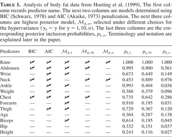
To amplify the preceding point of how the prior can impact model selection, and to help fix ideas, consider Table 1. The table is based on a highest posterior probability analysis of the body fat data of Hoeting et al. (1999). The data analyzed consist of n = 251 subjects, with each subject being measured for percentage of body fat. Also recorded are the age, weight, height, and 10 other body circumference measurements for the individual. As in Hoeting et al. (1999), we use body fat for the response in our regression model. The remaining 13 measurements are predictors for predicting body fat (see column 1 of Table 1 for a list of these variables). Note that with 13 predictors there is a total of 213 = 8,192 models, thus making an all-subsets highest posterior model search feasible.
Analysis of body fat data from Hoeting et al. (1999). The first column records predictor name. The next two columns are models determined using BIC (Schwarz, 1978) and AIC (Akaike, 1973) penalization. The next three columns are highest posterior model, , selected under different choices for the hypervariance (γk = γ for γ = 1,10,n). The last three columns are the corresponding posterior inclusion probabilities, pk,γ. Terminology and notation are explained later in the paper.

Listed in columns 4 through 6 of Table 1 are the highest posterior models selected under various prior specifications. Models were computed under a nonscaled spike and slab hierarchy with a uniform model prior (terminology will be spelled out later in the paper). The three models correspond to different values for the prior variance (hypervariance) of the βk coefficients. As can be seen, as the hypervariance γ increases, the highest posterior model quickly moves from a model larger than the Akaike information criterion (AIC) selected model to a model even sparser than the one selected using the Bayesian information criterion (BIC). This shows how sensitive highest posterior model selection can be to the choice of prior. Another interesting point, and one that came as somewhat of a surprise to us, is the relationship model size has with respect to γ. Typically, large hypervariances in spike and slab models are used to elicit a prior belief that a coefficient is informative. In contrast, Table 1 suggests that large hypervariances induce sparse models under highest posterior model selection, thus going in the opposite direction in which priors are typically chosen. Later we provide a theoretical explanation for this curious property.
Last, consider the final three columns of Table 1, which list the posterior inclusion probabilities for the three sets of priors used. Close inspection shows that the highest posterior model nearly coincides with the median model, that is, the model formed by choosing predictors k with pk,γ ≥ 0.5. This is interesting because it suggests that our theory, which takes advantage of the equivalence of the two models under orthogonal designs, may apply reasonably well even in highly correlated settings such as the one considered here.
1.3. Organization of the Paper
The paper is organized as follows. Section 2 introduces notation and the concept of total risk for variable selection. Section 3 introduces spike and slab models and formally defines the highest posterior model and the median model. Section 4 studies the asymptotic selection performance of the highest posterior model, and Section 5 makes use of a local asymptotic argument. Section 6 introduces the idea of rescaled spike and slab hierarchal models and studies their asymptotic selection performance and impact rescaling has on appropriate choice of priors. Section 7 presents a detailed simulation for studying performance of the procedures. Section 8 finishes with a discussion. The Appendixes supply proofs of results and a discussion of the asymptotics for null and full models.
2. NOTATION
The problem of selecting variables in the linear regression setting can be recast formally as a model selection problem using the following notation. For each subset α ⊆ {1,…,K}, let βα be the components of β that are indexed by the elements of α. One can think of βα equivalently in terms of the underlying model associated with it, which we call

. Formally, this model is defined as

where xi,α are the components of xi indexed by α (this notation of extracting coordinates indexed by α will be used repeatedly throughout the paper). When we think of βα, we will think of this interchangeably as either α or

. We define

to be the size of

or, equivalently, the number of variables in βα.
For example, for (1), which is often referred to as the full model, α = {1,…,K} and Kα = K. The other extreme model, the null model denoted by

, corresponds to α = [empty ] and the model

defined as

The size of the null model is K[empty ] = 0.
2.1. The True Model
Let β0 = (β1,0,…,βK,0)′ denote the true value for β. We indicate the true model by

, or just α0, where α0 are the indices of the nonzero coefficients of β0. Throughout it is assumed that

is neither the null nor the full model. In other words, it is assumed that

Such an assumption might seem at odds with our choice of prior (to be discussed shortly), which allows for the posterior to concentrate on both the null and full models. Our reason for assuming (3) is primarily for ease of presentation of asymptotic results. As a convenient way of summarizing the behavior of the highest posterior model our asymptotic results are cast in the form of comparisons of posterior model probabilities for overfit and underfit models relative to

(this style of presentation is common in the model selection literature; see, e.g., Shao, 1993; Zhang, 1993a). Unfortunately, for the notion of an overfit and underfit model to make sense, we must exclude the case when

is either the full or the null model. See, however, Appendix B for how our results are adjusted when (3) is violated.
2.2. Total Risk
To measure performance of a model selection procedure, we introduce the notion of total risk. The total risk is essentially a composite loss function under zero-one loss misclassification. To explain this, first note that a variable selection procedure can always be recast as a decision rule. If

is the model selected by the procedure, the corresponding decision rule is

, where

Let δk,0 = 1 if and only if βk,0 ≠ 0. We define the total risk for a model selection procedure

as

We say that a variable selection procedure

is total risk consistent if

. Notice that this is equivalent to the statement that the model estimator is consistent,

However, the measure of total risk is more meaningful for finite samples, as it provides a way of comparing procedures in terms of misclassification rates. See Ishwaran and Rao (2003, 2005a, 2005b) for further details. Throughout the paper we use total risk as a measure of performance.
3. BAYESIAN HIERARCHY
In this section we introduce a spike and slab framework that will be used to define our highest posterior model selection procedure,

. The properties of this selection procedure under the data generating mechanism (1) will then be explored in Section 4.
Two ingredients are required in specifying the spike and slab framework. The first involves specifying the prior used for the model space, which we will denote by π. This is chosen so that

for each model α and

(the sum being over all possible 2K models). The second ingredient is the likelihood structure used for modeling each regression problem

. This is specified by making use of a Bayesian hierarchy.
Section 3.1 discusses our choice for π in detail and how the resulting hierarchy is related to a popular class of models referred to as spike and slab models. Here we discuss the likelihood for

. This is based on a normal-normal conjugate hierarchical model. For each nonnull model

, we assume that

where Y = (Y1,…,Yn)′, Γα is the diagonal matrix extracted from Γ using only those coordinates in α, and Γ = diag{γ1,…,γK} where 0 < γk < ∞ are prespecified hypervariances. Typically {γk} are selected to reflect a prior belief in a coefficient. Large γk values induce large posterior values for βk and reflect a belief that the coefficient is informative, whereas small values give small βk coefficients and indicate a prior belief that the coefficient is noninformative.
Although a normal-normal hierarchical structure makes sense for nonnull models, special allowance has to be made for the null model

. To properly accommodate model (2), we assume

In both (4) and (5),

is assumed to be some consistent estimator for σ2. The rationale for introducing

in the hierarchy (4) rather than taking a more traditional approach of introducing σ2 as a Bayesian parameter with a prior is that it greatly simplifies our analysis. However, this is not to say that there is a loss in inferential capability in doing so. For example, Ishwaran and Rao (2005a) introduced both

and a Bayesian parameter σ2 in their setup and found only small incremental improvements in their selection procedure due to the inclusion of σ2.
3.1. Spike and Slab Models
For π we use an independence prior of the form

where 0 < wk < 1 are prespecified probabilities reflecting the prior belief that a coefficient is nonzero. Independence priors are a popular choice in Bayesian variable selection procedures, in both orthogonal and nonorthogonal settings, because they are easy to specify and simplify computations (Clyde, DeSimone, and Parmigiani, 1996; George and McCulloch, 1993, 1997; Hoeting et al., 1999; Smith and Kohn, 1996). One common choice for (6) is to set wk = ½ for each k. This gives

for each α and is often referred to as an indifference, or uniform, prior. More elaborate setups that involve a prior for wk are also used (Ishwaran and Rao, 2005a). However, we will not discuss these here.
When π is specified by (6), the hierarchy (4) and (5) can be written more compactly using a multivariate normal scale mixture distribution for β. Let bk ∼ Bernoulli(wk) be independent Bernoulli random variables. That is,

The vector b = (b1,…,bK)′ can be uniquely mapped to a specific α model. Thus, if we use the informal notation of denoting a degenerate multivariate normal by using zero values for the variance, then (4)–(6) can be more compactly expressed as

When written this way, the hierarchy (7) is often referred to as a spike and slab model (Ishwaran and Rao, 2005a, 2005b).
3.2. The Highest Posterior Model
It is widely believed that the highest posterior probability model possesses optimal model selection properties. As we show shortly this may not be the case at all. To define this model, observe by Bayes theorem that the posterior probability for a model

is

where

is the marginal density for Y under

. The model

is said to be the highest posterior model if

Equivalently,

is the highest posterior model if

Notice that under a flat prior for π this indicates that the highest posterior model has a Bayes factor that is greater than or equal to one over all model comparisons.
3.3. The Median Model
The issue of whether the highest posterior model is appropriate for inference was partially considered in Barbieri and Berger (2004). There it was shown in orthogonal settings that the optimal model from a Bayesian predictive viewpoint was not the highest posterior model but the median model. The median model can be defined formally as follows. Let Δk = {α : k ∈ α} denote the set of all models containing variable k. The model

is said to be the median model if

where pk is the posterior inclusion probability defined by

In other words,

is the model containing variables that appear with at least 50% posterior probability over all models.
The optimality result for the median model hinges on the definition of predictive optimality. This was defined as follows. For each α, let

be the posterior mean for β from

. For convenience we write

as a K-dimensional vector by setting coordinates not in α to equal zero. Let

be the BMA estimator for β from (7). Then,

Let

be the BMA predictor and

the predictor for

. The model

is said to be predictively optimal if

where ∥·∥ denotes the

-norm and the expectation is over Y with respect to the BMA predictive distribution. Thus,

is the single model whose prediction is closest to the BMA in an

-sense.
Although Barbieri and Berger (2004) illustrated several settings where the median model and highest posterior model differed, they also showed interesting examples where they coincided. Arguments given by Barbieri and Berger (2004) show in fact that spike and slab models of the form (7) are examples where the two approaches are equivalent.
THEOREM 1 (Barbieri and Berger, 2004). The highest posterior model and the median model coincide for spike and slab models of the form (7).
We come back to Theorem 1 later when we more closely examine the expression for the posterior inclusion probabilities (8) (in fact, we will provide an independent proof of a similar result; see Theorem 5). For now, it is enough to note the two procedures are identical and in particular that their total risks are equal. That is,

where

and

denote the decision rules for the highest posterior and median models, respectively.
4. SOME PRELIMINARY ASYMPTOTIC RESULTS
To present our asymptotic findings we follow Shao (1993) by categorizing models into two types depending upon whether they contain all the nonzero values of β0 or not (see also Nishii, 1984). The two categories of models are


Category I models are underfit incorrect models that exclude at least one nonzero coefficient. Note that a Category I model may include regressors whose coefficients are truly zero. On the other hand, Category II models consist of the true model

, the model with the smallest dimension, in addition to all models containing

as a subset. These latter models are overfit in the sense that they include all nonzero coefficients plus at least one truly zero coefficient. In Shao (1993, 1996) it was shown that one could not consistently recover the true model by minimizing the estimated prediction error using leave-one-out cross-validation or bootstrapping. Although the method distinguishes Category I models from Category II models, and therefore does not underfit, it cannot distinguish between Category II models in the limit, and therefore it overfits asymptotically. See also the papers by Stone (1977a, 1977b), who drew similar conclusions about cross-validation. Also see Geweke and Meese (1981); Hannan and Quinn (1979); Shibata (1976) for similar results in terms of Akaike's criteria.
Perhaps not surprisingly, the highest posterior model does not suffer from the inconsistency of the previously mentioned procedures. When Bayesians use normal hierarchical models for model selection they are often implicitly taking advantage of a BIC penalization, and this penalization makes it possible to discern the true model from other Category II models, thus avoiding overfitting asymptotically. In fact, we show in the following theorem that the highest posterior model is consistent (for more on BIC-like consistency in linear regression see Geweke and Meese, 1981; Nishii, 1984; Rao and Wu, 1989; Schwarz, 1978). However, although these results may appear promising, we find some undesirable properties.
THEOREM 2. Assume that {εi} are independent such that

,

, and

for some M < ∞. Assume that

. If (1) represents the data model and (7) the Bayesian model used for defining the posterior model selection procedure

, then the following conditions hold.
(i)

.
(ii) If

is a Category II model and

a Category I model,

(iii) If

and

are Category I models,

(iv) If

and

are two distinct Category II models such that Kα = Kα′,

Moreover,

if γ1 = ··· = γK and π is uniform.
Part (i) of Theorem 2 shows that highest posterior model selection is asymptotically consistent, but results (iii) and (iv) suggest suboptimal finite-sample performance. Consider result (iv), which pertains to Category II models. A careful inspection of the proof of the theorem (see equation (A.1) in the proof) shows that if α is a Category II model,

where C(α,α0) is a finite constant depending upon the prior. The dominating term in the expression is a BIC-like penalty of order log(n) that ensures, at least asymptotically, that the highest posterior model will identify the true model

over all other Category II models. However, for a fixed sample size n, there is a trade-off between the BIC penalty and the other terms in the expression, making it possible for

to equal some Category II model other than

.
Given this, it is of interest to consider what the distribution of π(α|Y) might look like over the space of Category II models. This would provide some insight into the behavior of

over this space. Result (iv) provides some answers. For example, the result shows that under a uniform model prior and equal hypervariances no model has a posterior probability dominating Category II models of the same dimension.
Under such a setting, this would suggest that if the highest posterior model selects a Category II model, such selection is approximately uniform from a class of Category II models of the same dimension (note that this is only an informal argument as result (iv) is not conditional on the behavior of

). Each instance of selecting a Category II model results in excess variability due to estimating zero coefficients of the true model. One way to mitigate this effect would be to use an estimator that averages over models from the same contour. However, the highest posterior model does not take advantage of model averaging, and thus we expect it would perform suboptimally when compared to procedures that use model averaging for selection (for examples of such procedures, see Ishwaran and Rao, 2003, 2005a, 2005b).
Result (iii) is also of concern in finite samples. As is well known, BIC penalization often leads to underfitting in practice, and thus for a fixed sample size, it is more than likely that the highest posterior model will be a Category I model. Result (iii) shows that over Category I models,

is asymptotically larger over those models with large

-coefficient norms. Thus, over Category I models, the highest posterior model could easily favor small models with high signal coefficients (again, this is only an informal argument as result (iii) is not conditional on the behavior of

). Although this might not impact prediction error performance, in terms of variable selection it is undesirable to select a small high-signal model over one with almost the same

-coefficient norm containing many small nonzero coefficients. Thus, in a finite-sample setting the highest posterior model may have large total risk.
5. LOCAL ASYMPTOTICS
The tendency for the highest posterior model to favor smaller models can be studied more carefully by using a local asymptotic argument. We look at its behavior in the setting when coefficients shrink to zero at an n−1/2 rate. This will indicate how the highest posterior model might perform in a finite-sample setting in which all coefficients are small.
For our analysis we assume that we have a triangular array of observations. That is, we assume that the true data generating mechanism is

where for each n, {εni : i = 1,…,n} are independent random variables with mean 0 and variance σ2. In (10), the true βn parameter is βn,0 = σn−1/2β0.
THEOREM 3. Assume that for every n, {εni : i = 1,…,n} satisfy the same conditions as {εi} in Theorem 2. If (10) represents the data model, and (7) the Bayesian model used for defining the posterior model selection procedure

, then under the same conditions for xi as in Theorem 2 the following conditions hold.
(i) For any two models

and

such that Kα < Kα′,

In particular,

because

.
(ii) If π is uniform and

and

are any two models such that Kα = Kα′,

where Zk are independent and identically distributed (i.i.d.) N(0,1) random variables.
Part (i) of Theorem 3 shows that the highest posterior model is inconsistent under a local asymptotic framework and therefore cannot be uniformly consistent. Moreover, part (i) shows that asymptotically,

will be larger over small models, which in combination with part (iii) of Theorem 2 suggests that the highest posterior model will tend to favor small models if many of the true coefficients have small values. This favoring of smaller models coincides with what is often seen using BIC. In fact, the phenomenon (i) where the null model is preferentially selected under a sequence of shrinking alternatives is known to be true generally for any pointwise consistent model selection procedure (see Leeb and Pötscher, 2005, Rmk. 4.4). Also see Leeb and Pötscher (2007) and Yang (2005) for more discussion on why consistent model selection procedures can perform poorly in finite samples.
Part (ii) of Theorem 3 shows over models of the same size that the posterior probability involves a delicate interplay between the true size of a coefficient and the prior hypervariance. In particular, notice that if γk is small for a given predictor k, then

will become large if k ∈ α, whereas if γk is large, then

is much smaller. This is quite curious, and undesirable, because it is counterintuitive to the spike and slab framework. The hypervariances in spike and slab models are designed so that large γk values reflect a prior belief that a covariate is informative, whereas small values reflect a belief that the variable is noninformative. In fact, recall how this counterintuitive result was found earlier in Table 1. Theorem 3 provides a reasonable explanation for why this occurs.
6. RESCALED SPIKE AND SLAB MODELS
Recently Ishwaran and Rao (2005b) discussed the role shrinkage plays in spike and slab models for high-dimensional variable selection. They introduced the notion of a rescaled spike and slab model, arguing that such models are desirable because of their property of maintaining a shrinkage effect in the limit. The effect of rescaling was used by Ishwaran and Rao (2005b) in tandem with a spike and slab hierarchy involving continuous bimodal priors. Although Ishwaran and Rao (2005b) considered a more delicate setup than here, the impact of rescaling nevertheless still holds, and it is of interest to study this.
In the context considered here, the rescaled spike and slab version of (7) is defined as follows:

where

. Rescaling amounts to replacing Y with an n1/2 scaled value and then replacing the variance in the hierarchical model with the value n.
6.1. Inclusion Probabilities
The following theorem provides an explicit characterization of the posterior inclusion probability for a variable. Define

This represents the signal contained in the data for the regression coefficients. Let

denote the posterior inclusion probability for k under (11).
THEOREM 4. Under the rescaled spike and slab model (11) we have

where dk = γk/(γk + 1). This should be compared to the posterior inclusion probability under the nonscaled model (7):

where

.
Theorem 4 shows that pk* and pk differ significantly over the zero coefficients. Under the conditions of Theorem 2,

and

if k is a nonzero coefficient, but if k corresponds to a zero coefficient,

, whereas, because the effect of γk does not vanish under rescaling, pk* has the following distributional limit:

6.2. Asymptotic Results
From these results it is tempting to conclude that it is better to use a nonscaled model (7). However, in the following theorem we show that rescaling helps to correct some problems seen for the highest posterior model. Our proof takes advantage of a perfect cancellation of a BIC penalty appearing in the expansion of the log of the posterior model probability. Although the trade-off is that the highest posterior model selected is no longer risk consistent, the flip side is that the method no longer breaks down in the local asymptotic case.
THEOREM 5. Under the Bayesian model (11) the following conditions hold.
(i) The highest posterior model and the median model are equivalent.
(ii) Fixed-parameter asymptotics: results (ii) and (iii) for Theorem 2 hold, where in (iii) replace β0 by D1/2β0 for D = diag{d1,…,dK}.
(iii) Local asymptotics: under the conditions of Theorem 3, if π is uniform and

and

are any two models,

Parts (i) and (ii) are essentially similar to the nonscaled case. It is under the local asymptotic setting, however, where we start to see differences between the two methods. Part (iii) shows that the highest posterior model no longer concentrates on the null model; in fact, notice the presence of dk in the limiting probability on the right. If the true value of a coefficient is zero, and γk is selected moderately small, then the value Zk2 = (βk,0 + Zk)2 is appropriately down weighted by the value dk. The presence of dk, therefore, discourages selection of models with zero coefficients. Notice also the presence of log(γk + 1) appearing in the limit on the right. This differs from the nonscaled case where a log(γk) term was found. Now a small hypervariance 0 < γk < 1, which might be associated with a coefficient thought to be noninformative, no longer heavily favors selection of models with k ∈ α.
6.3. The Impact of Rescaling
The preceding argument implicitly applies to a paradigm where coefficients are shrinking to zero. To further study the relationship between the prior and highest posterior model selection under rescaling, we exploit the equivalence between the highest posterior model and the median model. By Theorem 4, the posterior inclusion probability satisfies pk* ≥ ½ if and only if ξk,n2 ≥ ψ*(γk,wk), where

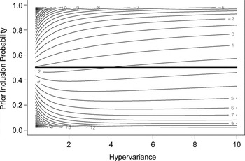
To understand how pk* varies in terms of these two parameters, we plotted the contour values of ψ*(γ,w) over a range of γ and w values. See Figure 1.

Contour plot of ψ*(γ,w) as a function of the hypervariance, γ, and prior inclusion probability, w. Note that ψ*(γ,w) is positive for small values of w and becomes negative as w increases to one. The thick line is horizontal value w = ½ and identifies contour values for the function ψ*(·,0.5).
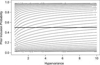
The thick line superimposed on the figure identifies the contour values for the function ψ*(·,0.5), which corresponds to the use of a uniform prior for π. For example, note how the line lies between the values of 2 and 3 when γ = 10, whereas its value is approximately 1 when γ is small. Compare this to the nonscaled setting. By Theorem 4, a predictor k is selected if and only if

, where

Figure 2 plots the contour values of this function over γ and w for n = 50 and σ2 = 1. The two plots confirm the mitigation of underfitting effects due to rescaling. Even for the small sample size illustrated in Figure 2, one can see how much larger the contour values are compared to Figure 1. For example, under a flat prior, the contour value for small γ values is more than 3 as compared to near 1 under rescaling. It is clear that nonscaled highest posterior model selection will tend to favor smaller models.

Contour plot of ψ(γ,w,n,σ2) for n = 50 and σ2 = 1. The thick line is horizontal value w = ½ and identifies contour values for the function ψ*(·,0.5,n,σ2).
Rescaling also allows the γk to be set in a more intuitive way. Consider what happens if wk = ½. If βk,0 is nonzero, then using a large value for γk shows that k will be selected with high probability because ξk,n2 will eventually be larger than ψ*(γk,0.5), which will be relatively small in comparison. This is exactly what we would like, because large γk values are used to elicit a belief that a covariate is informative.
On the other hand, consider what happens if βk,0 = 0. Now if we select γk to be small, ψ*(γk,0.5) ≈ 1. Thus, if βk,0 = 0, the predictor k will be selected with asymptotic probability

. Although this appears too large, and brings into doubt whether γk should be chosen this way, one should note if βk,0 is nonzero, but very small, then k will be selected with roughly the same probability. Thus, although one pays a price in overfitting if the coefficient is truly zero, there is a built-in robustness to misspecification. In fact, this is exactly the same effect discussed in Section 6.2 that keeps the rescaled highest posterior model from breaking down in a local asymptotic setting.
Figure 1 also indicates how the highest posterior model might be affected by the underlying size of the model. Consider the case when π is chosen such that wk = w for some hyperparameter w > 0 reflecting overall size or model complexity. The preceding discussion shows how to choose γk in a meaningful way when w = ½. Namely, we use small values for covariates we expect to be noninformative and large values for informative covariates. This type of calibration also applies when the value for w < ½ and the model is anticipated to be sparse. In fact, now the use of small γk values to indicate noninformative predictors makes even more sense. On the other hand, if w > ½ is large, then we run into calibration problems. Now ψ*(γ,w) can be negative for all values of γ. Clearly overfitting will occur, and there is no sensible way of selecting γk. This suggests that highest posterior model selection might operate best under rescaling only under sparse settings.
7. BREIMAN SIMULATIONS
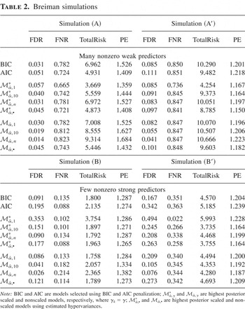
In this section we use simulations to study the empirical performance of highest posterior model selection under both the scaled and nonscaled settings. Our simulations followed those used by Breiman (1992). Specifically, data were generated by taking εi to be i.i.d. N(0,1) variables, and covariates xi were simulated independently from a multivariate normal distribution such that

and

, where 0 < ρ < 1 represents a correlation parameter. All simulations involved K = 14 predictors with a sample size of n = 50.
We considered four sets of simulations, (A), (B), (A′), and (B′), reflecting different correlation values ρ and different values for βk. For simulation (A), 12 of the 14 predictors were chosen to be nonzero. All coefficients were set to the same small value, this being chosen such that the theoretical R2 value for the model was 0.5 (for a discussion of this point, see Breiman, 1992). Thus, simulation (A) reflects a setting involving many nonzero weak predictors. In contrast, simulation (B) was designed to reflect a setting with few nonzero strong predictors. Of the 14 predictors, only six were chosen to be nonzero. Of these, two had the same large value; the other four had the same medium-sized value. The size of coefficients was selected so that the large coefficients were 2.4 times larger than the medium-sized ones and such that the theoretical R2 = 0.75. Both simulations (A) and (B) were based on a correlation of ρ = 0, thus reflecting an orthogonal design setting. On the other hand, simulations (A′) and (B′) used ρ = 0.9, reflecting a highly correlated design. Excepting this, simulation (A′) was the same as (A), and simulation (B′) was the same as (B).
Each of the four simulations was repeated 1,000 times independently. For each experiment we kept track of the false discovery rate (FDR), false nondiscovery rate (FNR) and total risk performance (TotalRisk) of a procedure. The FDR and FNR are the false discovery and false nondiscovery rates defined as the false positive and false negative rates for those coefficients identified as nonzero and zero, respectively. The TotalRisk equals the total number of falsely identified nonzero coefficients and falsely identified zero coefficients. Also computed was the prediction error performance (PE) of a procedure. This was defined as the mean square error of the estimated predictor computed over the original data when compared to a freshly drawn set of Yi responses using the original xi values.
Highest posterior model selection (both scaled and nonscaled) was investigated under a uniform model prior for π. Hypervariances were set to γk = γ, where three different values for γ were considered: γ = 1,10,n (this is similar to what was done in Table 1). Additionally, we introduced a hybrid procedure based on preselected hypervariances. Prior to estimating the highest posterior model we ran the spike and slab Gibbs sampler outlined in Ishwaran and Rao (2005b). This was done using both scaled and nonscaled responses. We then used the posterior means of γk estimated from the Gibbs sampler as the hypervariances used for highest posterior model selection. Note that a different set of hypervariances and a different set of highest posterior models were estimated for the scaled and nonscaled settings. Finally, in addition to examining highest posterior model selection, we also kept track of models selected using BIC and AIC penalization. These are the models with lowest BIC and AIC penalties over all models. The results for all these procedures are recorded in Table 2. Values reported are averaged values from the 1,000 simulations.
Breiman simulations

Our conclusions are summarized as follows:
- In simulations (A) and (A′), total risk performance for highest posterior model selection, and also for other measures of performance, degrades as γ increases. This is true for both the scaled and nonscaled cases. This is because the simulations reflect a setting where almost all coefficients are relatively small and so the optimal way to select γ would be to choose a small value. If γ is large, estimated models are too small, and performance suffers. Notice also the mitigation effects of rescaling. This is seen by the better total risk performance due to a lower FNR brought on by a less aggressive tendency to underfit—particularly evident here because of the weak underlying signal.
- The opposite effect is seen for simulations (B) and (B′) under rescaling. Now highest posterior model performance improves as γ increases. This is because in these sets of simulations only six coefficients are nonzero, two being large, the other four nonzero coefficients having moderate size. As γ increases estimated models become small and approach the true model. This backfires for nonscaled models though, because sparse models are approached very rapidly as γ becomes larger. Performance degrades in this setting because models are just too small and false negative rates too high. This behavior could have been predicted from Figure 2, where contour values under a uniform prior (i.e., the thick line) can be seen to increase quickly with increasing γ. As a result, only a very strong signal can be detected.
- Total risk performance and PE for rescaled highest posterior model selection is better than in nonscaled selection in almost all examples. This is true when comparing models for the same hypervariance or when comparing models based on preselected hypervariances.
- Total risk performance and PE for rescaled highest posterior model under preselected hypervariances,
, is better than AIC and BIC in almost all examples. The exception occurs in (B), where BIC is best with respect to total risk. In this particular scenario, BIC appears to discourage overfitting enough without inducing too much underfitting. Interestingly,
 is highly competitive in PE with BIC even in this situation. It is also interesting to note that BIC is no longer better thanin the correlated case, (B′).
- The results for simulations (A′) and (B′) are in tune with those found for (A) and (B). This suggests that our theory may also apply to correlated settings, at least approximately.


8. DISCUSSION
In this paper we have shown rigorously that underfitting using the highest posterior model occurs because of a BIC-like penalization term appearing in the log-posterior model probability. Various limiting probabilities were given in simple closed form expressions to help quantify what this means in practice. These kinds of specific details are not often found in the literature (one nice example is Zhang, 1993b, where rates at which over- and underfitting occur were established within the context of fixed-penalty information criteria). Our results show that underfitting is much worse than first thought—that the highest posterior model will tend to favor the smallest models with high signal coefficients among the group of underfit models for finite samples. This was further amplified by a local asymptotic argument that showed that the highest posterior model will eventually concentrate on the null model in cases where true coefficients are all weak.
We proposed a remedy for this by rescaling the responses and suitably altering the Bayesian hierarchy. Highest posterior model selection under the resulting rescaled spike and slab models, although no longer risk consistent, will be more evenly balanced, and the problems of underfitting will be substantially mitigated. In addition, calibration of the γk can be done in a way that is intuitively consistent with the spike and slab hierarchy. Interestingly though, under nonsparse prior settings, things break down because there is no sensible way to calibrate the γk. Here, regardless of how the γk are set, overfitting will be the result. This suggests that there is a disconnection between the general use of the highest posterior model for model selection and the manner in which hyperparameters in the prior are chosen.
One promising alternative that does not suffer from these problems is model selection based on the posterior mean from a rescaled spike and slab hierarchical model. Specifically, let

denote the posterior mean for β from (11). Taking advantage of conjugacy and orthogonality, one can show that

Therefore,

Proper calibration of priors is now no longer difficult, even for the nonsparse setting. For example, using the notation of Section 6.3, suppose that the model complexity value is w > ½. If γk is chosen to be small for zero coefficients and large for nonzero coefficients, then pk* will be nearly one for all coefficients. However, the posterior mean, because it includes the shrinkage effect γk/(γk + 1), will shrink the value of pk* and consequently will be small for zero coefficients while still being large for nonzero coefficients.
Thus, selection based on using the posterior mean will be free from calibration problems in all settings. In fact, effective strategies for model selection using the posterior mean from rescaled spike and slab models have already been developed (Ishwaran and Rao, 2005b). These operate by extending the hierarchy to include a continuous bimodal prior for the γk and provide automatic adaptive estimation of the γk (recall how the effectiveness of such values was demonstrated in the Breiman simulations). The resulting model averaged posterior mean estimates coupled with hard thresholding are then used for selection. A detailed theoretical treatment and empirical validation supporting the use of the posterior mean can be found in Ishwaran and Rao (2003, 2005a, 2005b) for the interested reader.
APPENDIX A: Proofs
Proof of Theorem 2. With some algebra, and using Xα′Xα = nIα, one can show for each nonnull model

,

where ξk,n is defined as in (12), dk,n is defined as in Theorem 4, and

Therefore, if

and

are two distinct nonnull models,

Taking logs, and keeping in mind

, it follows that

Notice that the first term on the right-hand side represents a BIC penalty that penalizes larger models by a factor of log(n). There is a trade-off in size, though, involving the sums containing ξk,n2. These terms can be evaluated using a central limit theorem. In particular, it follows that if βk,0 = 0, then

, whereas if βk,0 ≠ 0, we have

. Thus over the nonzero coefficients, ξk,n2 is order Op(n), which becomes the dominant term in (A.1). Because of this, it is clear that each Category II model

will have exponentially larger posterior probability than any Category I model

, and thus (ii) follows (for the case of the null model α′ = [empty ], simply substitute 0 for Kα′ and remove all sums involving α′ in (A.1)). Over Category II models,

Because (A.2) only involves zero coefficients, the term is order Op(1), and thus the BIC penalty becomes the dominant term in (A.1). Because this penalty penalizes larger models, deduce (i). Furthermore, if Kα = Kα′, and if π is uniform and γ1 = ··· = γK, then (A.1) reduces to (A.2) over Category II models. If

and

are distinct, the sum on the right-hand side of (A.2) converges in distribution to ½ of the difference between two i.i.d. χk2 variables (with 2k equaling the total number of distinct zero coefficients in both models). From this deduce the second part of (iv). The first part of (iv) follows because (A.1) reduces to (A.2) plus an incidental finite constant if π and γk are not necessarily uniform.
Finally to prove (iii), observe that

if βk,0 ≠ 0. These variables represent the dominating terms in working out the desired probability and are of order n. Dividing (A.1) throughout by

, and using

, it follows that the event on the left-hand side of (9) occurs if and only if

Proof of Theorem 3. A triangular central limit theorem (Serfling, 2002) shows under the local asymptotic setting (10) that

where

. Also, under (10), identity (A.1) continues to hold. Thus, whenever Kα ≠ Kα′, the BIC penalty is the dominant term in (A.1), and part (i) follows. If Kα = Kα′, the BIC term disappears. Part (ii) follows upon using

. █
Proof of Theorem 4. By definition,

In the proof of Theorem 2 we have shown for each nonnull model

,

where C is a constant independent of α (in fact

). Assume that α ∈ Δk. Let α−k = α − {k}. Removing the contribution from the variable k, we have

Furthermore, because of the special nature of the prior, if we extract the contribution of k, we have

, and therefore

There is a 1:1 mapping between Δk and Δkc. In particular, observe that

Hence, if we extract the term in (A.4) depending upon k, the ratio of the sums in (A.3) simplifies to

Therefore, pk−1 = 1 + Rk. By carefully tracking back through the arguments, substituting n for

and Y* for Y, one can deduce a similar result for pk*. █
Proof of Theorem 5. We first prove (i) by showing that the posterior model probability factorizes into a product of the underlying posterior inclusion probabilities. To do so we will make use of the product rule of probability. For convenience we will use products hereafter to indicate intersection of sets. Let Δ be any set of models such that Δk ∩ Δ ≠ [empty ] and Δkc ∩ Δ ≠ [empty ]. We have

By arguing as in the proof of Theorem 4 (cf. eqn. (A.3)), one can show this equals pk*. The other relevant case for Δ occurs when Δk ∩ Δ = {k} and Δkc ∩ Δ = [empty ]. In other words, Δ = {[empty ],{k}}. Let Rk* be the value of Rk when n is substituted for

and dk for dk,n. Then, arguing as before, it is not hard to see that

From this, and the product rule of probability, deduce that for any model

It is clear that the median model is the model that maximizes the posterior model probability.
Now to prove (ii) and (iii). Using arguments similar to Theorem 2 deduce

Argue as in the proofs of Theorems 2 and 3 to deduce (ii) and (iii). █
APPENDIX B: Asymptotics for Null and Full Models
We now indicate how our main asymptotic results are affected when assumption (3) is violated. That is, if

is allowed to be either the null or full model.
- Consider first the case when
is the full model. Then the space of Category II models is simply. Because this space contains only one model, part (iv) of Theorem 2 no longer applies. However, the remainder of the theorem continues to hold. Theorems 3 and 5 also continue to hold. This can be seen by noting that the key expression (A.1) applies in the full model case.
- Now suppose
is the null model. Then the space of Category I models is defined to be empty, and all models are of a Category II type. Hence, in Theorem 2, parts (ii) and (iii) no longer apply because the Category I model space is empty. The remainder of the theorem continues to hold, however. This follows by noting that (A.1) applies to the null model by setting the relevant dimension to zero and removing all sums involving the null model. Theorem 3 continues to apply, although the highest posterior model is obviously no longer inconsistent. Theorem 3 in fact is noninformative in the null model case because the point was to consider the setting in which coefficients may be small and nonzero. Theorem 5 also continues to apply except for part (ii), which applies to Category I models. Note that in Theorems 3 and 5 if α or α′ is set to the null model, simply replace the relevant sum with the value 0. Also note that βk,0 = 0 for each k.