1. Introduction

Ice age-dating is one of the principal steps in ice-core data interpretations and paleoclimatic reconstructions. There is no universal and/or standard procedure to determine depth– age relationships in polar ice sheets at deep-drilling sites. The latter question is of primary importance for the record 3600 m deep ice core retrieved from the Antarctic ice sheet at Vostok station (Reference PetitPetit and others, 1999) above the vast subglacial lake.

Applicability of sophisticated two- and three-dimensional (2-D and 3-D) thermomechanical ice-flow models (Reference RitzRitz, 1992; Reference Ritz, Rommelaere and DumasRitz and others, 2001) for solving this problem suffers significantly from uncertainties in initial and input data: mainly in glacier bottom conditions and past accumulation rates. Nevertheless, the detailed analysis by Reference Parrenin, Jouzel, Waelbroeck, Ritz and BarnolaParrenin and others (2001) shows that the modeling of ice-sheet dynamics becomes a useful tool for ice age prediction if a priori chronological information is used to fit the model parameters. Although different sources of age markers and dated time series have their own specific errors, they may be considered reliable constraints if, in combination, they deliver statistically valid and independent estimates of ice age at various depth levels. The inverse Monte Carlo sampling method (e.g. Reference Mosegaard and TarantolaMosegaard and Tarantola, 1995; Reference MosegaardMosegaard, 1998) is especially helpful in this case (Reference Parrenin, Jouzel, Waelbroeck, Ritz and BarnolaParrenin and others, 2001) to fit the ice-sheet model on average, uniformly vs depth, although without putting excess weight on local fluctuations of the simulated depth–age curve caused by uncertainties in environmental conditions, reconstructed ice accumulation and other paleoclimatic characteristics. From this point of view, even simplified ice-flow models (e.g. Reference Salamatin and RitzSalamatin and Ritz, 1996; Reference Hondoh, Shoji, Watanabe, Salamatin and LipenkovHondoh and others, 2002) may be appropriate for incorporating the principal laws of ice-sheet dynamics into the ice-core dating procedure.

Among different depth–age relationships developed for Vostok, the geophysical metronome time-scale (GMTS), extended in Reference Salamatin, Vostretsov, Petit, Lipenkov and BarkovSalamatin and others (1998a) and Reference Salamatin and HondohSalamatin (2000) to the maximum depth 3350 m of the Vostok ice-core isotope record covering four interglaciations, represents the so-called orbitally tuned chronologies. It is based on correlation of the isotopic temperature signal with the geophysical-metronome Milankovich components of past local surface temperature variations inferred from the borehole temperature profile. Possible errors and uncertainties in GMTS are discussed elsewhere (Reference Salamatin, V.Ya. Lipenkov, Barkov, Jouzel, Petit and RaynaudSalamatin and others, 1998b; Reference Salamatin and HondohSalamatin, 2000), and its overall average accuracy was estimated as ±3.5–4.5 kyr. Orbital ice-age control points used in Reference Parrenin, Jouzel, Waelbroeck, Ritz and BarnolaParrenin and others (2001) as model constraints coincide (to within ±2 kyr) with the corresponding GMTS ages.

Another paleotemperature proxy signal spanning >500 000 years is available from the calcite core (DH-11) in Devils Hole, Nevada, U.S.A. (Reference WinogradWinograd and others, 1992, Reference Winograd, Landwehr, Ludwig, Coplen and Riggs1997). The principal advantage of this δ¹⁸O record is that the dense vein calcite provides material for direct uranium-series dating (Reference LudwigLudwig and others, 1992), with the standard errors increasing from 1 to 7 kyr with time up to 400 kyr BP. In addition, the signal may be influenced by different hydrological factors. In particular, a systematic underestimation of the ages determined, on the order of several thousands of years, may take place due to the groundwater travel time through the aquifer (Reference WinogradWinograd and others, 1992; Reference Landwehr and WinogradLandwehr and Winograd, 2001). Nevertheless, the correlation of the Vostok ice-core deuterium–depth signal with the Devils Hole record (see US Geological Survey open-file report 97792 at http://pubs.water.usgs.gov/ofr97–792) can also be considered as an independent approach to dating the longest paleoclimate archive from central Antarctica (Reference Landwehr and WinogradLandwehr and Winograd, 2001).

The possibility of using various gas studies of Vostok ice cores for relative dating (correlation) with other Antarctic, Greenland or deep-sea core climatic records is not considered here, because of the additional errors which arise from the uncertainty in the gas–ice age difference, preventing better constraints on the ice age. These questions are addressed by Reference Salamatin, V.Ya. Lipenkov, Barkov, Jouzel, Petit and RaynaudSalamatin and others (1998b) and with a deeper focus by Reference Parrenin, Jouzel, Waelbroeck, Ritz and BarnolaParrenin and others (2001).

Thus, the principal goals of our study are (1) to combine the above sources of chronological information in order to constrain ice-flow model parameters, reducing to a minimum systematic errors in the glaciological time-scale based on simulations of the ice-sheet dynamics in the vicinity of Vostok station, (2) to deduce the average age–depth relationship consistent with different approaches to the ice-core dating within the upper 3350 m, and (3) to extend the model predictions at Vostok to the deeper bottom part of the glacier.

2. Model Description and Parameterization

Here we use a simplified 2-D approach to ice flowline modeling developed for ice age predictions by Reference Hondoh, Shoji, Watanabe, Salamatin and LipenkovHondoh and others (2002). We introduce the longitudinal coordinate s as a distance from the ice divide along a reference flowline. The flow tube configuration is described by its relative width H(s) and the ice equivalent thickness Δ(s, t) depending on time t. The vertical coordinate ζ is the relative distance from the glacier bottom expressed in equivalent thickness of pure ice and normalized by Δ. The paleoclimate is characterized by the surface ice mass balance b(s; t).

An ice-particle trajectory passing through a given point (s0; ζ0) can be approximated as

where is the normalized spatial distribution of the accumulation rate along the flowline. Observations by Reference SiegertSiegert and others (2001), Reference Bell, Studinger, Tikku, Clarke, Gutner and MeertensBell and others (2002) and preliminary temperature simulations indicate that the basal melting is not likely to occur along the Vostok flowline, and its influence on the ice-sheet dynamics is neglected.

Temporal variations of b and Δ are described in the following parametric form:

Here b0 is the present-day ice mass balance at the site under consideration (s = s0), and Δ0(s) is the present-day glacier thickness (in ice equivalent) along the flowline. The last exponential term in the first of Equations (2) describes the past changes in precipitation traditionally correlated to the inversion (isotopic) temperature in accordance with Robin

(1977) and Reference RitzRitz (1989, Reference Ritz1992). The accumulation-rate variations in central Antarctica are linked by means of the exponential factor ηb and the deuterium/inversion-tempera-ture slope CT to the ice-core isotopic content ratios δD corrected for past changes in the oxygen isotope composition of ocean water δ¹⁸O_sw (Reference SowersSowers and others, 1993; Reference Bassinot, Lebeyrie, Vincent, Quidelleur, Shackleton and LancelotBassinot and others 1994). Deviations δD and δ¹⁸O_sw in Equations (2) are referenced to their present-day values. For relatively small ratio ηb/CT the accumulation-rate variations become linearly dependent on isotopic temperatures. A more sophisticated relationship between the inversion temperature and the deuterium content in ice, directly taking into account the water-vapor source temperature variations, has recently been suggested by Reference Cuffey and VimeuxCuffey and Vimeux (2001). Correspondingly, as emphasized and explained by Reference JouzelJouzel and others (2003), the correction of δD to the sea-water isotopic content δ¹⁸O_sw enters the transfer function with the factor of 4.8 rather than 8 (used here for consistency with the earlier studies). As shown below in section 4, this leads to slight overestimation of the isotope/temperature gradient CT.

Ice-sheet thickness fluctuations δΔ(t) in the second of Equations (2) are reconstructed after Reference Salamatin and RitzSalamatin and Ritz (1996). The latter model for δΔ was verified and its tuning parameters γb and γl were constrained on the basis of the 2-D thermomechanically coupled model of Antarctic ice-sheet dynamics (Reference RitzRitz, 1992). These results have also been recently supported by 3-D simulations (Reference Ritz, Rommelaere and DumasRitz and others, 2001). As follows from Reference Salamatin and RitzSalamatin and Ritz (1996), γl is inversely proportional to the modified Glen flow-law exponent β, which takes account of the vertical temperature gradient (Reference LliboutryLliboutry, 1979). It decreases from 2.5 to 2.1 when β increases from 10 to 20; γb can be fixed as 0.56.

The ice-particle motion in the vertical direction is predicted (Reference Hondoh, Shoji, Watanabe, Salamatin and LipenkovHondoh and others, 2002) from an ordinary differential equation with respect to ζ = ζ(t)

with b, Δ and s related to ζ and t by Equations (1) and (2). By definition, σ is the proportion of the total ice-flow rate through the reference flow tube due to plastic (shear) deformation of the glacier body, 0 ≤ σ ≤ 1.

Finally, the ice age t0 of the ζ0 level at s = s0 is determined by equality ζ(t0) = ζ0, where ζ(t) is the solution of Equation 1 at the initial condition ζ|t=0 = 1. A depth–age relationship used initially for the ice-core deuterium record in Equations (2) is corrected through iterative modeling.

The ζ coordinate is expressed via depth h (after Reference Salamatin and HondohSalamatin, 2000) as:

where Cs is the surface snow porosity and γs the exponential densification factor.

Although computation of the depth–age relation is finally reduced to solving a ‘one-dimensional’ Equation 1, the dating procedure itself is originally based on a 2-D ice-flow model, and thus inherits the principal laws of ice-sheet dynamics, taking into account the geographic conditions and climate changes. One might argue (Reference Hondoh, Shoji, Watanabe, Salamatin and LipenkovHondoh and others, 2002) that such a simple approach to ice age prediction is rather rough and includes several tuning parameters. However, even much more complicated 2-D or 3-D models cannot resolve the uncertainties about ice-deformation mechanisms and glacier sliding over the bedrock. Neither the past climate changes nor the present-day geographical situation are reliably known. Thus, the simplicity of the above model, with explicitly introduced parameters that have clear physical meaning, is its principal advantage and makes it a useful instrument in glaciological studies.

A schematic map of the Vostok lake vicinities adapted after Reference Siegert and RidleySiegert and Ridley (1998) is presented in Figure 1a. The reference ice flowline passing through Vostok station and the ice-flow tube are depicted by the arrowed bold solid and dashed lines, respectively. They are drawn perpendicular to the surface elevation contours (Reference Siegert and RidleySiegert and Ridley, 1998) for the grounded part of the ice sheet and after Reference SiegertSiegert and others (2001) and Reference Bell, Studinger, Tikku, Clarke, Gutner and MeertensBell and others (2002) over the lake. The relative ice-flow tube width H(s) vs distance s from Ridge B is shown in Figure 1b. The smoothed present-day ice-sheet thickness Δ0(s) along the Vostok flowline also plotted in the figure is deduced from the airborne radio-echo sounding profile (Reference SiegertSiegert and others, 2001) and the detailed geographic data (Reference Bell, Studinger, Tikku, Clarke, Gutner and MeertensBell and others, 2002; Reference Tabacco, Bianchi, Zirizzotti, Zuccheretti, Forieri and Della VedovaTabacco and others, 2002; Reference StudingerStudinger and others, 2003). The spatial distribution of the normalized mass balance is drawn in Figure 1b with account of the mass-balance enhancement factor 1.65

Fig. 1.

Geographic conditions around Vostok station. (a) A schematic map of the Vostok lake vicinities adapted after Reference Siegert and RidleySiegert and Ridley (1998) and the Vostok flowline considered in the ice age simulations (see text). (b) The present-day ice-sheet thickness Δ₀ together with the relative ice-flow tube width H and normalized accumulation rate b vs distance measured from Ridge B along the reference flowline in (a).

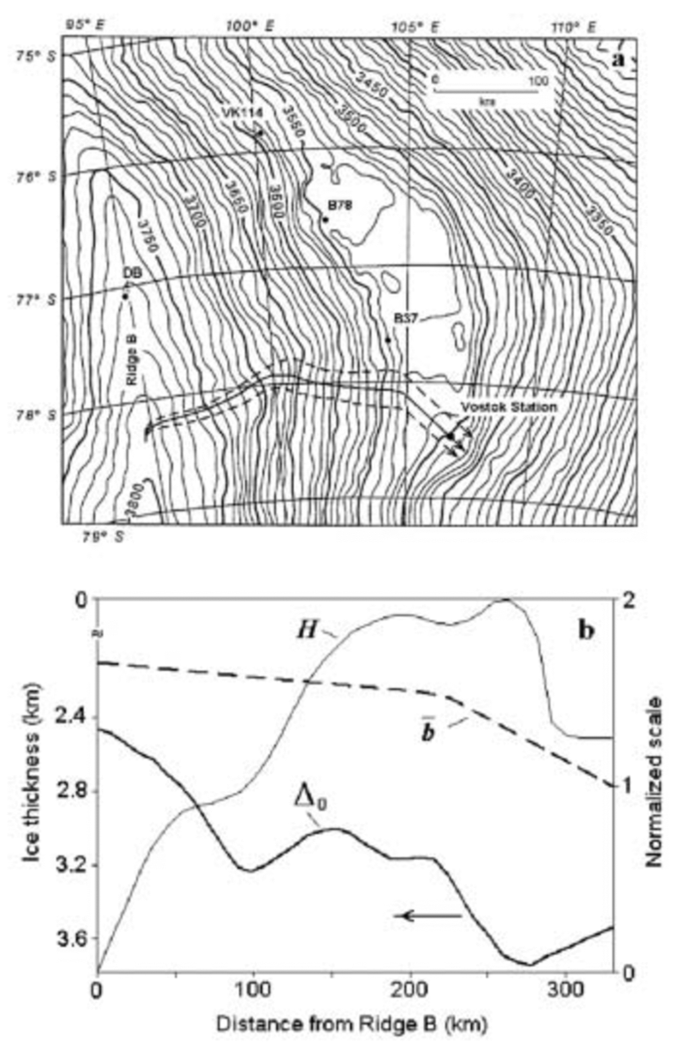
The values and a priori ranges of the basic model parameters considered in computations are given in Table 1. The present-day accumulation rate at Vostok was assumed on the basis of several studies (Reference Barkov and LipenkovBarkov and Lipenkov, 1996; Reference Ekaykin, Lipenkov, Barkov, Petit and MassonEkaykin and others 2001, Reference Ekaykin, Lipenkov, Petit and Masson-Delmotte2003), with the lower and upper bounds determined as the mean values over last 200 and 50 years, respectively. The ice densification and flow parameters are estimated and discussed in Reference Salamatin and HondohSalamatin (2000) and Reference Barkov, Vostretsov, Lipenkov and SalamatinBarkov and others (2002). The exponential approximation of the snow–firn density profile (c _s and γ_s in Equation 1) is additionally confirmed by the new data (Reference Ekaykin, Lipenkov, Petit and Masson-DelmotteEkaykin and others, 2003).

Table 1.

Ice-flow model parameters for Vostok area

estimated by Reference JouzelJouzel and others (1993) for Ridge B at the location of the Dome B ice core marked as DB in Figure 1a. The shape of the curve is taken as similar to the smoothed accumulation-rate profile along the traverse to Vostok passing through sites B37, B78 and VK114 (see Fig. 1a), with ice accumulation rates measured by Reference Lipenkov, Ekaykin, Barkov and PourchetLipenkov and others (1998). Although such a projecting procedure is rather schematic, the resulting normalized distribution compares in general to the spatial accumulation-rate changes which might be derived from tracing the internal radar layers along the Vostok ice flowline (Reference Leysinger Vieli, Siegert and PayneLeysinger Vieli and others, 2004).

3. Ice-Core Ages Imported From Paleoclimatic Signals

Vostok ice age-dating procedures considered in this study are substantially based on the deuterium ice-core record (Reference PetitPetit and others, 1999) plotted in Figure 2a together with its parabolic spline approximation (Reference Salamatin and HondohSalamatin, 2000). The GMTS results directly from correlation of the smoothed isotopic signal with the geophysical metronome (Milankovich cycles of the local surface temperature variations) inferred from the deep borehole temperature profile at Vostok (Reference Salamatin, Vostretsov, Petit, Lipenkov and BarkovSalamatin and others, 1998a, Reference Salamatin, V.Ya. Lipenkov, Barkov, Jouzel, Petit and Raynaudb; Reference Salamatin and HondohSalamatin, 2000). The metronome is presented in Figure 2b. The GMTS correlation pairs, ages and depths of the respective climatic events (peaks and troughs) identified in the metronomic and isotopic signals are depicted in Figure 3a by filled circles. It should be noted that the ice-core analysis (Reference PetitPetit and others, 1999) revealed some indications of ice-flow disturbances below 3310m at Vostok. This reduces the confidence in identification and correlation of the two last extrema in the isotope record, although their ages display the right tendency to increase with depth. The eight orbital ice-age control points used in Reference Parrenin, Jouzel, Waelbroeck, Ritz and BarnolaParrenin and others (2001) are shown (filled triangles) in Figure 3b together with other age markers as deviations from a common reference time-scale explained below in section 4. They are in close agreement with linear interpolations between the GMTS correlation points: the age deviation is <1 kyr on average.

Fig. 2.

Paleoclimatic signals used to constrain the ice-flow model and the simulated (glaciological) ice age–depth relationship at Vostok. (a) Vostok ice-core deuterium record (dots) and its parabolic spline approximation (solid line). (b) Geophysical metronome inferred from the borehole temperature profile at Vostok. (c) DH δ¹⁸O record (thin line) and its parabolic spline approximation (bold line).

Fig. 3.

Different ice age-datings at Vostok. (a) Best-fit glaciological time-scale (thin solid line) and average ice age–depth relationship (bold line) compared with GMTS (filled circles) and DHVTS (open circles) age–depth correlation points used for constraining the ice-flow model. The inset shows upper and lower extensions of the glaciological time-scale to 3530 m depth, 10 m above the boundary with the accreted lake ice. Rectangles and numbers are the climatic stages discerned in the Vostok dust concentration record. (b) The deviation of the linearly interpolated GMTS and DHVTS ages (filled and open circles, respectively) from a reference time-scale (zero line) chosen as the mathematical expectation (best fit) of the sampled chronologies at Vostok. Filled and open triangles are the respective control points from Reference Parrenin, Jouzel, Waelbroeck, Ritz and BarnolaParrenin and others (2001) and Reference Landwehr and WinogradLandwehr and Winograd (2001). The dashed lines are the SD bounds of the age–depth curves selected through the Monte Carlo sampling procedure.

Next, we applied the parabolic spline approximation to the Devils Hole (DH) paleoclimatic record (Reference WinogradWinograd and others, 1992) as plotted vs time in Figure 2c. The extrema in the Vostok deuterium–depth curve are now identified with the corresponding maxima and minima discerned in the smoothed DH signal. Thus, another independent series of 31 DH age markers is transferred to the Vostok ice core (see open circles in Fig. 3a). These points are also presented in Figure 3b together with 12 age–depth pairs (open triangles) chosen by Reference Landwehr and WinogradLandwehr and Winograd (2001) for importing the DH chronology. The standard deviation of the latter set of Vostok age estimates from the linear interpolations between the newly deduced correlations of the climatic events is about 1.6 kyr. Hence, the DH-to-Vostok time-scale (DHVTS) based on the spline representation of the DH isotope paleorecord is consistent with the earlier age–depth correlation established in Reference Landwehr and WinogradLandwehr and Winograd (2001).

Remarkably, the mean difference between GMTS and DHVTS within the age interval of their overlap (60–430 kyr) is practically zero (∼0.2 kyr). The periods of constant-sign deviations do not exceed several times 10⁴ years. This indicates that there is no significant systematic (long-term) shift of one time-scale with respect to another. At the same time, the mean-square (standard) deviation (SD) is rather high, ∼7.6 kyr, and maximum mismatches reach 10–15 kyr (see Fig. 3a and b). Reference Bassinot, Lebeyrie, Vincent, Quidelleur, Shackleton and LancelotCuffey and Vimeux (2001) give a good illustration of how sensitive the details of isotope paleorecords are to changes in their water-vapor sources and, hence, to their origins. In addition, the drift of snow-accumulation waves (megadunes) on the ice-sheet surface (Reference Van der Veen, Mosley-Thompson, Gow and MarkVan der Veen and others, 1999) and post-depositional effects may also cause specific perturbations in ice-core isotopic records on time-scales of thousands of years, as revealed by Reference Ekaykin, Lipenkov, Barkov and PetitEkaykin and others (2002, Reference Ekaykin, Lipenkov, Petit and Masson-Delmotte2003) and discussed by Reference Waddington, Steig and NeumannWaddington and others (2002) for shorter periods. The geophysical metronome, as a sum of Milankovich cycles, originally assumes a quasi-linear response of the Earth’s climate to orbital forcing with fixed constant frequencies and phase shifts, disregarding ‘climatic noise’ and possible non-linearities (Reference Salamatin, V.Ya. Lipenkov, Barkov, Jouzel, Petit and RaynaudSalamatin and others, 1998b; Reference Salamatin and HondohSalamatin, 2000). Thus, the above estimates may be understood if the ages from two different series with statistically independent perturbations (errors) of 4–6 kyr are intercompared. These conclusions are important and allow us to use the GMTS and DHVTS age–depth correlation points to constrain the ice-flow model in the Vostok area on average, with minimum systematic errors in ice age predictions to a depth of 3350 m.

4. Ice-Flow Model Constraints and Glaciological Time-Scale

Equations (1–4) were first validated on the best-guess time-scale simulated for the Vostok ice core by Reference Parrenin, Jouzel, Waelbroeck, Ritz and BarnolaParrenin and others (2001) with the use of the general 2-D model for Antarctic ice-sheet dynamics (Reference RitzRitz, 1992). For an appropriate choice of parameters, the simplified model (1–4) reproduced the ice age–depth curve with accuracy no worse than 1.5 kyr. Such a close agreement and earlier applications of this approach for ice-core dating at Dome Fuji (Reference Hondoh, Shoji, Watanabe, Salamatin and LipenkovHondoh and others, 2002) and Vostok (Reference Barkov, Vostretsov, Lipenkov and SalamatinBarkov and others, 2002) support the idea that Equations (1–3), being properly constrained, describe the ice age–depth distribution in an ice sheet on a macroscale level with an accuracy comparable to that of the thermomechanical 2-D and 3-D models. Approximations (1) and (2) and the smoothed geographic data in Figure 1 do not capture the fine spatial and temporal variations of the flow tube which will be a source of high-frequency noise in the simulated age–depth relation. These perturbations are not correlated with the ice age-dating errors introduced by use of the geophysical metronome or the DH paleoclimatic signal. Consequently, we expect that the modeled (glaciological) time-scale at Vostok, fitted to the two depth–age relationships of different origins (GMTS and DHVTS), might be considered as another source of ice age estimates with minimum systematic error, though containing independent short-term distortions.

Here we follow Reference Parrenin, Jouzel, Waelbroeck, Ritz and BarnolaParrenin and others (2001) and employ the inverse Monte Carlo sampling procedure (e.g. Reference Mosegaard and TarantolaMosegaard and Tarantola, 1995; Reference Mosegaard and TarantolaMosegaard, 1998) to study the sensitivity of the target function, the standard deviation of the glaciological time-scale from GMTS and DHVTS, to five tuning parameters: the present-day accumulation rate at Vostok, b0; the deuterium-content/inversion-temperature temporal slope, CT (or equally ηb/CT); the location of the ice-sheet western grounding line at Vostok lake, sl with σ = 0 for s0 > s > sl; the boundary of the Ridge B highlands, sh with relatively high σ∼0.5–1.0 for 0 < s < sh; and the shear-flow rate factor upstream of the lake in the intermediate zone σl (σ = σl, sh < s < sl). The plausible a priori ranges for these values are given in Table 1. Several series of computational experiments were conducted to perform the resolution analyses with different combinations of the model parameters at different constraints. The best-fit estimates, obtained through the Monte Carlo method and discussed below, are summarized in Table 2.

Table 2.

Estimates of the model tuning parameters deduced through the Monte Carlo sampling method for β = 10 (β = 20)

Preliminary tests showed unequal uncertainty levels of GMTS and DHVTS, with the latter age fluctuations around the fitted model predictions 1.4–1.7 times higher than those of GMTS. The respective absolute values of the ‘Gaussian noise’ SD assumed in the likelihood function of the Metropolis algorithm were estimated as 4.7–4.3 and 6.6– 7.4 kyr. Although these uncertainties include the modeling errors, they are close to the claimed accuracies of GMTS and the DH age dating. In each computational experiment, about 103–(5×103) uncorrelated chronologies were selected at 35% level of acceptance by the Monte Carlo scheme. Depending on a frequency of selection related to the number of inferable parameters and assumed ranges of their variation, the total number of tested time-scales was 105–106.

In general, the resolution analysis performed by means of the random-walk sampling shows that the resulting posterior probability density in the space of the ice-flow model parameters is not unimodal and has an extended domain of global maximum. This means that feasible variations of some parameters can be counterbalanced by a priori accepted changes in the others. Only additional restricting information on the model parameters can lead to a more definite estimation. Nevertheless, all best-fit chronologies found in different computational series are practically indistinguishable and fell within 5.9 ± 0.3 kyr limits of the standard deviation from the GMTS and DHVTS age markers. This implies that the model (1–4) is sufficiently flexible and the simulated depth–age relationship can be uniquely constrained by the available chronological information at plausible values of the tuning parameters. The thin solid line in Figure 3a depicts the best-fit glaciological time-scale. It converges to the mathematical expectation of the sampled (selected) age–depth curves. Deviations of the GMTS and DHVTS ages from the statistical mean, best-fit, ages (zero line) are plotted in Figure 3b. The dashed lines are the SD bounds of the tested chronologies. Since GMTS and DHVTS are used as model constraints, a certain apparent similarity of their fluctuations around the glaciological time-scale in Figure 3b should be assigned mainly to the short-term details missed in the modeled age–depth curve, and not to the systematic statistically correlated errors between the time-scales themselves.

With this result, let us discuss a posteriori information on the model parameters deduced through the Monte Carlo procedure. First, the deuterium/inversion-temperature slope C _T enters Equations (2) as a ratio to ηb, and its estimates automatically include all errors of the latter factor (Reference RitzRitz, 1992) as well as the general uncertainties of the assumed Reference RobinRobin’s (1977) geographic relationship. Hence, the obtained values of C _T cannot be directly interpreted in terms of the transfer function between the ice-core isotope content and inversion temperature. Furthermore, as clearly seen from Equation 1, for the major part of the ice sheet (for ζ > 0.1– 0.2) the ice age–depth distribution is mainly controlled by the ratio σ/(β + 1), and any change in β correspondingly influences the inferable values of σ. Therefore, in the basic series of computations, we fixed β = 10 in accordance with Reference Salamatin and RitzSalamatin and Ritz (1996).

Initial random-walk sampling over the complete set of five model parameters b0, CT, σl, sl and sh within the limits given in Table 1 revealed an important tendency that for any σ in the Ridge B highland area (0 < s < sh) the optimal position of sh was shifted towards 20 –25 km distance from the ice divide, and the ice age predictions above 3350m depth near Vostok station became insensitive to the σ values. Correspondingly, in further computational experiments we assumed sh = 20 km. Next, extremely low sensitivity of the modeled glaciological time-scale was observed with respect to the grounding-line location sl, with a very weak maximum of the sampling probability around 50–60km from Vostok, in full agreement with Reference Bell, Studinger, Tikku, Clarke, Gutner and MeertensBell and others (2002). Thus, sl was fixed as 275 km from Ridge B. After that, the reconnaissance resolution analysis was performed in the space of the three parameters (b0, CT and σl) within much wider ranges than the a priori bounds set in Table 1, for b0 from 1.4 to 2.4 cm a^–1 and for CT from 4 to 15‰˚C^–1. A 2-D map of the normalized probability density sampled by the Monte Carlo method on the b ₀–C _T phase plane is plotted in Figure 4a. It clearly shows that only the values of C _T∼5– 7‰˚C^–1 are consistent with the a priori estimates of b0∼2.15–2.4 cm a^–1 (see the bold-dashed outlined rectangle domain in Fig. 4a). The best fit becomes insensitive to the deuterium/temperature slope and shifts to unreasonably low values of the present-day accumulation rates B0 ∼1.6– 1.9 cm a^–1 for CT ∼8–15‰˚C^–1. As can easily be understood, this corresponds to the limiting case of Equations (2) at CT →∞ when temporal variations of the accumulation rate are suppressed and B0 tends to its long-term average value (∼1.3–1.5 cm a^–1). Finally, the localized area of the feasible b0 and CT variations was additionally explored with the random-walk sampling. As might be expected, the inverse procedure revealed in this case a nearly uniform distribution of the sampling probability density vs b0, a ‘sharp’ unimodal histogram for CT and a clearly resolved maximum in the histogram for σl. All three distribution functions are presented in Figure 4b. The corresponding estimates of the model parameters are given in Table 2. The best fit was found at a standard deviation of the glaciological time-scale from GMTS and DHVTS (the target function value) of about 5.8 kyr. The inferred values of CT ≈ 5.6 ± 0.6‰˚C^–1 agree with previous results based on the borehole temperature analysis (Reference Salamatin, V.Ya. Lipenkov, Barkov, Jouzel, Petit and RaynaudSalamatin and others, 1998b) and preliminary simulations of the ice-sheet dynamics (Reference Barkov, Vostretsov, Lipenkov and SalamatinBarkov and others, 2002). This slope determines a deuterium-ratio–inversion-temperature relationship, which falls exactly midway between the bounds reconstructed by the inverse procedure in Reference Parrenin, Jouzel, Waelbroeck, Ritz and BarnolaParrenin and others (2001). The use of the correction factor 4.8 for the water-isotopic composition in the first of Equations (2), instead of 8, reduces the above estimates of CT by approximately 6% without influencing the ice dating. The best-fit present-day accumulation rate is found at its lower bound, 2.15cma^–1, and matches with the mean value, 2.2 ± 0.03cma^–1, calculated for the recent 200 years from the depths of the Tambora (Indonesia) eruption layer measured at Vostok in nine shallow boreholes and deep pits (Reference Ekaykin, Lipenkov, Petit and Masson-DelmotteEkaykin and others, 2003). Rather low values of σl 0.24 ± 0.1 are indicative of intense sliding over the glacier bed and/or soft-ice shear zone development in the basal layer. The former peculiarity could be the model artifact attributable to the substitution of the smoothed bedrock profile for the natural subglacial relief with high undulations (see Reference SiegertSiegert and others, 2001), while the latter is a realistic phenomenon observed in Vostok ice cores (Reference Lipenkov, Barkov and SalamatinLipenkov and others, 2000) and simulated by Reference Salamatin and MalikovaSalamatin and Malikova (2000). All these findings remained generally unchanged for β = 20 (see Table 2) at similar estimates of the model parameters, except for the expected increase in the shear-flow rate factor: σl ≈0.34 ± 0.2.

Fig. 4.

The a posteriori information on the ice-flow model parameters deduced through the Monte Carlo sampling procedure. (a) A map of the normalized sampling probability density on the b ₀– CT phase plain. (b) The histograms of the three principal model parameters: present-day accumulation rate b ₀ at Vostok, deuterium/inversion-temperature slope CT, and shear-flow rate factor σ _l explored in the bold-dashed outlined rectangle domain in (a).

5. Average Time-Scale: Discussion

The three depth–age relationships introduced and compared in the previous sections are uniformly consistent with each other to the maximum depth, 3350 m, of the Vostok ice core. The errors in these primary, basic time-scales differ in magnitude and by origin. On average, the uncertainty level of age dating can be predicted with a reduction compared to the standard deviation of the best-fit (glaciological) time-scale from GMTS and DHVTS: that is, not higher than 4.2 kyr. However, the latter estimate and the statistical validity of ice-core dating might be additionally improved if the difference in error levels is taken into account. For example, SD between the best-fit time-scale and GMTS is 4.3–4.7 kyr. Hence, the average accuracy of their mean ages is about 3.0–3.3 kyr. Accordingly, we assume that each of the three basic depth–age relationships has its own uncertainty level, and iteratively calculate the weighted mean time-scale using the running averaging procedure over a 4 kyr interval comparable with the average error level. The weights are taken inversely proportional to standard deviations of the basic chronologies from the resulting smoothed average curve. This condition yields converged normalized weighting coefficients of 0.44, 0.38 and 0.18 for the best-fit glaciological time-scale, GMTS and DHVTS, respectively, with the corresponding standard deviations from the mean ages equal to 2.2, 2.6 and 5.6 kyr. The latter estimates characterize the quality of different sources of chronological information and reveal the higher statistical validity (the lower error level) of the properly constrained glaciological time-scale. The bold line in Figure 3a shows the average time-scale. The deviations of the three basic time-scales from the average age–depth curve (zero line) are plotted in Figure 5a. The dot-dashed lines in the figure are the total standard error bounds of ±3.6 kyr which correspond to the upper estimate of the age uncertainty. Actually, the deduced error level of the best-fit glaciological time-scale, ±2.2 kyr, i.e. the weighted mean SD of all three chronologies, is thought to be a more reliable measure of the accuracy of the newly developed time-scale. The average age–depth relationship is presented in Table 3 together with the running weighted mean SD (errors) also shown in Figure 5b by dashed lines. Because of the ice-flow disturbances, the actual errors below 3310m may be higher, and question marks follow the respective SD estimates in Table 3. The average time-scale has also been substituted into Equations (2) to calculate the isotopic content of precipitation vs time and, thus, is additionally fitted through iterations.

Fig. 5.

Comparison of the average time-scale developed for the Vostok ice core with other time-scales of different origins. (a) The deviation of the three Vostok age–depth relationships, i.e. GMTS (linearly interpolated filled circles), DHVTS (linearly interpolated open circles) and the best-fit glaciological time-scale (bold line) from the averaged time-scale (zero line). The dot-dashed lines show the standard error bounds of the mean ages. (b) Deviation of the best-guess time-scale (Reference Parrenin, Jouzel, Waelbroeck, Ritz and BarnolaParrenin and others 2001) and GT-4 (Reference PetitPetit and others, 1999) from the average time-scale: bold (1) and thin (2) curves, respectively. Dotted lines are the running weighted mean SD bounds of ice ages from Table 3.

Table 3.

Average age–depth relationship for Vostok ice core and its theoretical extension to the boundary with the accreted lake ice

Both Figure 5 and Table 3 show non-uniform distribution of errors vs depth and age. The age uncertainties range from 0.25 to 3–4 kyr at maximum. Obviously, the highest errors are located around 110, 140, 180 and 360 kyr (1500, 2000, 2350 and 3170 m), mainly where the maximum mismatch between the Vostok and DH isotopic records and/or their chronostratigraphies is observed (see Fig. 3b and 5a). In all these cases, the best-fit glaciological depth–age relationship and GMTS agree with the average time-scale within the standard uncertainty bounds, and only the ages imported from the DH paleosignal display abrupt fluctuations with 2–2.5 higher amplitudes. To track such extreme variations of DHVTS by the ice-flow model, in simulations, we would need accumulation rates at least two times higher (or lower) than those predicted by the first of Equations (2), continuously during 25–50 kyr intervals. This seems unrealistic and most likely is due to the different origins of the Vostok and DH isotopic records.

In Figure 5b the average time-scale is compared to GT-4 and the best-guess time-scale developed for Vostok ice cores by Reference PetitPetit and others (1999) and Reference Parrenin, Jouzel, Waelbroeck, Ritz and BarnolaParrenin and others (2001). Both age–depth curves significantly, although within their accuracy limits, deviate from the average time-scale (zero line in Fig. 5b). Such a discrepancy may be a consequence of overtuning the ice flow in these other models to a limited (statistically non-representative) number of specific control points (e.g. see Fig. 3b).

We can now estimate the ice age at Vostok below 3350 m, although because of the ice-flow disturbances below 3310 m (Reference PetitPetit and others, 1999) such an attempt may be just a theoretical exercise. However, recent studies of the deepest part of the Vostok glacier ice (Reference simôesSimões and others, 2002) showed that the glacial stages 14 and 16 are still distinctly discernible in the dust concentration record within the depth intervals 3393–3405 and 3440–3455 m, respectively, and most likely that interglacial stage 17 covers the depth range 3457–3466 m. This suggests that the ice, at least to 3470m depth, has undergone only local perturbations. Hence, an extension of the time-scale toward the boundary with the accreted lake ice, to a depth of 3540 m, can provide an estimation of possible maximum variations of ice ages and the statistically expected age–depth distribution.

First we calculated the long-term average accumulation rate, 1.4 cm a^–1, at Vostok over four climatic cycles, using Equation 1 with the best-fit estimates of b0 and CT (see Table 2). Then, the best-fit glaciological time-scale has been continued in our simulations to 3530m depth, with the averaged accumulation rate assumed for the paleoclimatic history before 430 kyr BP. Predicted ice ages in the bottom part depend on the Ridge B highland boundary Sh and the shear-flow rate factor σh in this area (0 < s < sh), increasing with sh and σh. Parameter σh in the cold vicinities of Ridge B cannot be lower than °1 in the intermediate zone. Consequently, only the limiting values of σh = σ1 and σh = 1 have been tested in simulations at the lower (best-fit) and upper values of sh = 20 and 80 km, respectively. The latter estimate for sh is the maximum geographic constraint (see Fig. 1b). This was confirmed in preliminary computational experiments which showed low sensitivity of the best-fit glaciological time-scale (∼0.5 kyr) to sh within the above range and revealed an exponential increase in its standard deviation from GMTS and DHVTS from 6 to 17 kyr for higher sh values from 80 to 200 km. The computed respective lower and upper age bounds plotted in the inset in Figure 3a are obtained with the apparent creep index β =10 and for β linearly decreasing from 10 to 1 upstream from sh =80 km. Their arithmetic mean agrees with the average time-scale below 3310 m with an accuracy of about 1 kyr and continues it at the end of Table 3. The error estimates are the mean age deviations from the simulated bounds plus additional standard errors caused by averaging the past accumulation rates before 430 kyr BP and estimated to be ∼6 kyr. The maximum ice age at 3530 m could reach 1960 ± 1120 kyr, provided that the basal ice flow has not been disturbed. Higher values of β > 10 do not change the age estimates. The depth ranges of the stages 14, 16 and 17 suppositionally observed in the dust concentration record (Reference simôesSimões and others, 2002) and their durations estimated in Reference Bassinot, Lebeyrie, Vincent, Quidelleur, Shackleton and LancelotBassinot and others (1994) are shown as rectangles in the inset in Figure 3a and are in agreement with the theoretical upper bound.

6. Conclusion

Three different approaches to ice-core age dating are employed to develop an average age–depth relationship at Vostok. Firstly, the GMTS, extended in Reference Salamatin, Vostretsov, Petit, Lipenkov and BarkovSalamatin and others (1998a) and Reference Salamatin and HondohSalamatin (2000) to the maximum depth 3350m of the Vostok ice-core isotope record covering four interglaciations, is used as a so-called orbitally tuned chronology. It is based on correlation of the isotopic temperature signal with the geophysical metronome Milan-kovich components of past local surface temperature variations inferred from the borehole temperature profile. Another paleotemperature proxy signal spanning >500 000 years is available from the calcite core (DH-11) in Devils Hole (Reference WinogradWinograd and others, 1992, Reference Winograd, Landwehr, Ludwig, Coplen and Riggs1997). The principal advantage of this δ¹⁸O record is that the dense vein calcite provides a material for direct uranium-series dating (Reference LudwigLudwig and others, 1992). The correlation of the Vostok ice-core deuterium–depth signal with the DH record yields a second, independent, time-scale (DHVTS). Ice-flow modeling also becomes a useful tool for ice age prediction if a priori chronological information is used to constrain the model parameters. Here we base our study on a simplified 2-D approach to ice flowline simulations as described in Reference Salamatin and RitzSalamatin and Ritz (1996) and Reference Hondoh, Shoji, Watanabe, Salamatin and LipenkovHondoh and others (2002). Consequently, the modeled (glaciological) time-scale at Vostok fitted to the GMTS and DHVTS represents a third source of ice age estimates and incorporates the principal laws of ice-sheet dynamics into the ice-core dating procedure. The inverse Monte Carlo sampling method proves to be especially helpful for constraining the accumulation-rate reconstruction and ice-flow modeling to find the best-fit glaciological time-scale matched with the two other chronologies (see Table 2). General uncertainties of the above age estimates vary from 2 to 6 kyr on average and reach 6–15 kyr at maximum. Whatever the causes of these discrepancies might be, they are thought to be of different origins, with statistically independent errors. Thus, the average time-scale for the Vostok ice core down to 3350 m depth is deduced consistent with all three dating procedures within the standard deviation limits of ±3.6 kyr. The estimate of the actual accuracy of the developed average age–depth relationship should take into account the different error levels of the primary basic time-scales and is predicted as ±2.2 kyr on average. The constrained ice-sheet flow model allows, at least theoretically, extrapolation of the mean ice age–depth curve to the boundary with the accreted lake ice where the glacier-ice age at 3530m depth may reach (or even exceed) ∼2000 kyr.