Temperature profile of icy worlds

In our analysis, we shall assume that the object under consideration comprises a surface ice layer with an subsurface ocean situated below. For the sake of simplicity, we do not consider worlds where the outer layers consist of both ice and rock, which are believed to exist on some Solar system satellites (Schubert et al., Reference Schubert, Anderson, Spohn, McKinnon, Bagenal, Dowling and McKinnon2004; Nimmo and Pappalardo, Reference Nimmo and Pappalardo2016).Footnote ⁴ Our assumption of an ice envelope and a subsurface ocean implicitly assumes that the water content is sufficiently high to enable the existence of these two layers. However, it must be recognized that the water inventory of planets and satellites has been predicted to vary considerably (Raymond et al., Reference Raymond, Scalo and Meadows2007; Mulders et al., Reference Mulders, Ciesla, Min and Pascucci2015; Ciesla et al., Reference Ciesla, Mulders, Pascucci and Apai2015; Bergin et al., Reference Bergin, Blake, Ciesla, Hirschmann and Li2015), and hence the depth and existence of the subsurface ocean cannot be estimated a priori.

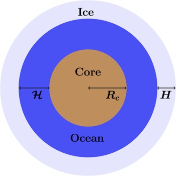
The planet's heat flux is assumed to arise from a combination of radiogenic and primordial (gravitational contraction) heating; on Earth, it is known that the former contributes approximately 50% of the total heat flux (The KamLAND Collaboration, 2011). The effects of tidal heating are assumed to be negligible in our model, unlike Europa and Enceladus (Barr and Showman, Reference Barr, Showman, Pappalardo, McKinnon and Khurana2009; Hussmann et al., Reference Hussmann, Choblet, Lainey, Matson, Sotin, Tobie and van Hoolst2010; Spencer and Nimmo, Reference Spencer and Nimmo2013; Choblet et al., Reference Choblet, Tobie, Sotin, Běhounková, Čadek, Postberg and Souček2017a) as well as some free-floating satellite–planet systems (Debes and Sigurdsson, Reference Debes and Sigurdsson2007), where tidal dissipation is expected to play an important role. In addition, we do not explicitly consider the heating due to serpentinization reactions that is anticipated to be quite significant on small worlds such as Enceladus and Mimas (Malamud and Prialnik, Reference Malamud and Prialnik2013). A schematic figure of the planet has been depicted in Fig. 1.

Fig. 1.

Schematic illustration of the planet with an ice envelope, a liquid water ocean and an inner rocky/metallic mantle and core.

We shall determine the thermal profile for the outer ice layer by assuming that the heat is transported via conduction, and not through convection. The latter depends on a wide range of properties for rocky and icy planets, such as the mass, ice grain size, availability of water and mantle rheology to name a few (Schubert et al., Reference Schubert, Turcotte and Olson2001; Barr and McKinnon, Reference Barr and McKinnon2007; Baraffe et al., Reference Baraffe, Chabrier, Fortney and Sotin2014) and the putative existence of bistable behaviour, multiple steady states, mixed heating and temporal evolution only serves to complicate matters further (Lenardic and Crowley, Reference Lenardic and Crowley2012; Korenaga, Reference Korenaga2017). In our own Solar System, it has been proposed that non-Newtonian creep mechanisms are responsible for convective shutdown on some dwarf planets and satellites with potential subsurface oceans (McKinnon, Reference McKinnon2006), such as Callisto and Pluto. It has also been suggested that the inclusion of contaminants (e.g. ammonia and salts), which lower the melting point of ice, may influence the degree of convection (Abbot and Switzer, Reference Abbot and Switzer2011; Travis et al., Reference Travis, Palguta and Schubert2012).Footnote ⁵ Despite these complexities, provided that the shell's thickness or the heat flow is sufficiently high, thermal convection will occur on such objects, and the thickness of the ice layer can be estimated accordingly (Hussmann et al., Reference Hussmann, Sohl and Spohn2006; Fu et al., Reference Fu, O'Connell and Sasselov2010).

Given the above assumptions, the temperature profile is determined via Fourier's law

(1)$$ {\cal Q} + \kappa \displaystyle{{d T} \over {d r}} = 0, $$

where ${\cal Q}({r})$ is the geothermal heat flux at radius r (in units of W/m²), T ≡ T(r) denotes the temperature at radius r, and κ is the thermal conductivity of ice. Note that $\kappa = \cal {C}/T$ with $ {\cal C} \approx 651$ W/m based on equation (3.11) of Petrenko and Whitworth (Reference Petrenko and Whitworth1999). The heat flux ${\cal Q}(r)$ within the ice envelope can be expressed as

(2)$$ {\cal Q} = \displaystyle{{Q} \over {4 \pi r^2}} \times \displaystyle{{r^3} \over {R^3}} = \displaystyle{{Q\, r} \over {4 \pi R^3}}, $$

where R is the radius of the planet, and Q represents the total internal heat flow from the planet to space (in units of W). Thus, the heat flux is given by the ratio of the heat flow within the enclosed region Q _enc and the area of this region (4π r ²). Note that Q _enc is approximately equal to 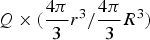$Q \times ( {{4 \pi} \over {3}}r^3/ {{4 \pi} \over {3}} R^3)$ and the second factor follows from the assumption that the heating sources are uniformly distributed throughout the planet's volume. Furthermore, we will make use of the ansatz

(3)$$ Q = \Gamma Q_\oplus \left(\displaystyle{{M} \over {M_\oplus}}\right)^\alpha, $$

where Q _⊕ is the internal heat flow of the Earth (The KamLAND Collaboration, 2011) and M is the mass of the planet, while Γ and α are free parameters. Note that both Q and Q _⊕ are implicitly time-dependent, as radiogenic heating declines exponentially with time. However, if we restrict the discussion to planets that were formed a few Gyr ago, it can be verified that Q changes merely by an order unity factor (Turcotte and Schubert, Reference Turcotte and Schubert2002) when only long-lived isotopes are taken into consideration. Our analysis has excluded short-lived isotopes (Neveu et al., Reference Neveu, Desch and Castillo-Rogez2017), but these elements can play a potentially important role in the thermal evolution of icy worlds.

Equation (3) is a generalization of the standard convention wherein Γ = 1 and α = 1. This choice amounts to stating that Q/M, namely the heating rate per unit mass (in W/kg) is constant (Valencia and O'Connell, Reference Valencia and O'Connell2009). For radiogenic heating, Q depends upon the mass of the rocky mantle – usually assumed to have a chondritic composition that contains the radioactive elements (Spohn and Schubert, Reference Spohn and Schubert2003) – which is not necessarily linearly proportional to the mass of the planet. Hence, there is no a priori reason for assuming α = 1. Similarly, since planets with metallicities different than that of Earth exist (Johnson and Apps, Reference Johnson and Apps2009; Buchhave et al., Reference Buchhave, Bizzarro, Latham, Sasselov, Cochran, Endl, Isaacson, Juncher and Marcy2014), it is therefore conceivable that the abundance of radionuclides may also vary accordingly; this variability is encapsulated in our model by means of the parameter Γ.Footnote ⁶ Alternatively, Γ can also be used to encapsulate the degree of heating from other sources (e.g. tidal dissipation).

We turn our attention to the planetary radius which can be determined through a mass–radius relationship. It is not possible to identify a single scaling since it depends on the composition, and is not always a power law (Seager et al., Reference Seager, Kuchner, Hier-Majumder and Militzer2007). Nevertheless, for the sake of simplicity, we assume

(4)$$ M = \lambda M_\oplus \left(\displaystyle{{R} \over {R_\oplus}}\right)^\beta, $$

where R is the planet's radius, with λ and β representing free parameters. The value of β is dependent both on the H₂O content and the mass, but λ ≈ 1 in most cases. We shall use β ≈ 3.3 for M ≲ M _⊕ (Sotin et al., Reference Sotin, Grasset and Mocquet2007) and β ≈ 3.8 for M ≳ M _⊕ (Valencia et al., Reference Valencia, Sasselov and O'Connell2007; Fu et al., Reference Fu, O'Connell and Sasselov2010).

Next, we solve (1) by imposing the boundary condition T(r = R) = T _s, where T _s denotes the temperature at the surface. The temperature profile is given by

(5)$$ \ln \left(\displaystyle{{T} \over {T_{{\rm s}}}}\right) = \displaystyle{{Q (R^2 - r^2)} \over {8 \pi {\cal C} R^3}}. $$

We are now in a position to determine the thickness of the ice layer. The phase-diagram of H₂O implies that the melting point of ice ranges between  ≈ 250 and 270 K provided that the pressure P is lower than 620 MPa (Choukroun and Grasset, Reference Choukroun and Grasset2007). As the temperature dependence is logarithmic in nature, we can assume a melting point of T _m = 260 K for pure ice. In contrast, the presence of ammonia (as a contaminant) can lower the melting point of ice to the peritectic temperature of 176 K; this corresponds to a 33% NH₃ concentration in the ocean (Leliwa-Kopystyński et al., Reference Leliwa-Kopystyński, Maruyama and Nakajima2002). The value of r at which T = T _m, denoted by R _m, is

(6)$$ R_{{\rm m}} = R \left[1 - \displaystyle{{8 \pi {\cal C} R} \over {Q}} \ln \left(\displaystyle{{T_{{\rm m}}} \over {T_{{\rm s}}}}\right)\right]^{1/2}, $$

and the thickness H of the ice layer is determined via H = R − R _m. Thus, we obtain

(7)$$ \displaystyle{{H} \over {R_\oplus}} = \left(\displaystyle{{R} \over {R_\oplus}}\right) \left(1 - \left[1 - 2.4 \times 10^{-3}\displaystyle{{\ln \Lambda} \over {\Gamma}}\left(\displaystyle{{R} \over {R_\oplus}}\right)^{1 - \gamma}\right]^{1/2}\right), $$

where we have introduced the auxiliary notation γ = αβ and Λ = T _m/T _s. By inspecting this formula, it is evident that H will decrease whenever Λ is reduced or Γ is increased for fixed values of R/R _⊕ and γ. Hence, provided that D > H, where D denotes the average water depth, the planet can host sub-surface oceans. As noted earlier, it is not possible to quantify D beforehand since the water content of the planet can vary widely.

As an example, let us suppose that the Earth were to be ejected into space. We obtain the surface temperature upon solving $\sigma T_{{\rm s}}^4 = {\cal F}_\oplus $, where $ {\cal F}_\oplus = 0.087$ W/m², and find that T _s ≈ 35 K. Hence, it follows that lnΛ ≈ 2 if we use T _m ≈ 260 K. Using this value in (7) along with Γ = 1 and R = R _⊕, we find H ≈ 15 km. The Earth's average water depth D _⊕ is ≈ 3.7 km (Charette and Smith, Reference Charette and Smith2010). Hence, it seems plausible that the Earth's oceans would be entirely frozen as per this model;Footnote ⁷ see also Laughlin and Adams (Reference Laughlin and Adams2000) for a related discussion of this question. If the Earth was ejected shortly after its formation, the geothermal heat flux could have been higher by a factor of order unity due to short-lived radionuclides and primordial heat. Hence, provided that the criterion Γ ≳ 4 was valid, the primordial Earth might have retained a global subsurface ocean if it had become a free-floating planet. For this value of Γ, we obtain H ≈ 3.75 km for the Earth, and the condition D _⊕ > H is satisfied since D _⊕ for the early Earth was approximately twice its present-day value (Korenaga, Reference Korenaga2008).

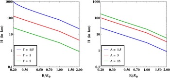
In Fig. 2, we have plotted H as a function of the radius for different values of the free parameters Γ and Λ. If we consider the case where the second term inside the square brackets of (7) is much smaller than unity, we can use the binomial theorem to obtain the following expression:

(8)$$ H \approx 7.6 \,{\rm km}\;\displaystyle{{\ln \Lambda}\over {\Gamma}} \left(\displaystyle{{R} \over {R_\oplus}}\right)^{2 - \gamma}, $$

and, for α = 1 in conjunction with the values of β discussed earlier, the condition γ > 3 is always satisfied. Hence, the thickness will be a monotonically decreasing function of the radius. Before proceeding further, it must be recognized that (7) is not valid for all values of R. This limitation arises since the quantity inside the square brackets must be positive (to ensure that that its square root is real). Hence, we find that the model has a lower bound (denoted by R _c) given by

(9)$$ \displaystyle{{R_{ {\rm c}}} \over {R_\oplus}} = \left(2.4 \times 10^{-3}\displaystyle{{\ln \Lambda} \over {\Gamma}}\right)^{1/(\gamma - 1)}, $$

and for the choices lnΛ ≈ 2 and Γ = 1, we obtain R _c ≈ 0.1 R _⊕. The value of R _c increases monotonically with Λ and decreases monotonically with Γ. On the other hand, we can assume that ${\cal Q}$ is constant in (1) along the lines of Abbot and Switzer (Reference Abbot and Switzer2011). We find that the solution resembles (8) except for the additional factor of Γ and a different power-law exponent.

Fig. 2.

Left panel: thickness of the ice shell as a function of the planet's radius for differing radionuclide concentrations (represented by Γ) and a fixed surface temperature arising from Earth's radiogenic heating (corresponding to Λ = 7.5). Right panel: thickness of the ice envelope for differing surface temperatures (encapsulated by Λ) and a fixed radionuclide concentration (Γ = 1).

Our analysis is not expected to yield accurate results for Europa and Enceladus since the effects of tidal dissipation are not included in our model. For instance, if we employ (7) with Γ = 1 and use Λ ≈ 2.5 for Europa, the resultant value of H is about a factor of 4 higher compared with more sophisticated predictions (Lunine, Reference Lunine2017).

Habitats for potential subsurface oceans

We briefly discuss some of the cases where subsurface oceans might exist.

Type B (involving objects bound to a star): When planets lie beyond the HZ of their host star, they can host sub-surface oceans (Ehrenreich and Cassan, Reference Ehrenreich and Cassan2007; Fu et al., Reference Fu, O'Connell and Sasselov2010). Examples within our Solar System include Europa and Enceladus, and it has been posited that water-rich extrasolar planets (Léger et al., Reference Léger, Selsis, Sotin, Guillot, Despois, Mawet, Ollivier, Labèque, Valette, Brachet, Chazelas and Lammer2004) such as OGLE 2005-BLG-390Lb may also fall under this category (Ehrenreich et al., Reference Ehrenreich, Lecavelier des Etangs, Beaulieu and Grasset2006). Two important points are worth noting at this stage concerning this class of planets.

• • The value of Λ can vary by an order of magnitude because Λ ≈  1–10. For instance, the average (morning/evening) surface temperature of Ceres is 168 K (Küppers et al., Reference Küppers, O'Rourke, Bockelée-Morvan, Zakharov, Lee, von Allmen, Carry, Teyssier, Marston, Müller, Crovisier, Barucci and Moreno2014), which leads to Λ ≈ 1.5 upon choosing T _m ≈ 260 K; a minimum of Λ ≈ 1.1 can be attained for Ceres at the subsolar point. Recent observations of carbonate deposits in the Occator crater on Ceres (de Sanctis et al., Reference de Sanctis, Raponi, Ammannito, Ciarniello, Toplis, McSween, Castillo-Rogez, Ehlmann, Carrozzo, Marchi, Tosi, Zambon, Capaccioni, Capria, Fonte, Formisano, Frigeri, Giardino, Longobardo, Magni, Palomba, McFadden, Pieters, Jaumann, Schenk, Mugnuolo, Raymond and Russell2016) and the detection of volatiles (Russell et al., Reference Russell, Raymond, Ammannito, Buczkowski, De Sanctis, Hiesinger, Jaumann, Konopliv, McSween, Nathues, Park, Pieters, Prettyman, McCord, McFadden, Mottola, Zuber, Joy, Polanskey, Rayman, Castillo-Rogez, Chi, Combe, Ermakov, Fu, Hoffmann, Jia, King, Lawrence, Li, Marchi, Preusker, Roatsch, Ruesch, Schenk, Villarreal and Yamashita2016; Combe et al., Reference Combe, McCord, Tosi, Ammannito, Carrozzo, De Sanctis, Raponi, Byrne, Landis, Hughson, Raymond and Russell2016) lend further credence to the possibility that this dwarf planet has/had a subsurface ocean on account of its relatively high surface temperature (Castillo-Rogez and McCord, Reference Castillo-Rogez and McCord2010). On the other hand, for trans-Neptunian objects (TNOs) such as Eris, it can be shown that Λ ≈ 10.

• • The HZ need not necessarily correspond only to a main-sequence star. Exoplanets with subsurface oceans (lying outside the HZ) could also exist around white dwarfs and brown dwarfs (Agol, Reference Agol2011; Barnes and Heller, Reference Barnes and Heller2013; Loeb and Maoz, Reference Loeb and Maoz2013), as well as post-main-sequence (Lorenz et al., Reference Lorenz, Lunine and McKay1997; Lopez et al., Reference Lopez, Schneider and Danchi2005; Ramirez and Kaltenegger, Reference Ramirez and Kaltenegger2016) and pre-main-sequence (Ramirez and Kaltenegger, Reference Ramirez and Kaltenegger2014; Luger and Barnes, Reference Luger and Barnes2015) stars.

If the Type B planet is not very far from its host star, the surface temperature can be estimated via

(10)$$T_{ {\rm s}} \approx 213 {\rm K}\left(\displaystyle{{1 - A} \over {0.36}}\right)^{1/4}\left(\displaystyle{{L_\star} \over {L_\odot}}\right)^{1/4} \left(\displaystyle{{a} \over {1 {\rm AU}}}\right)^{-1/2}, $$

where A is the albedo of the planet, L _★ denotes the luminosity of the host star, and a is the average star–planet distance. We have normalized 1 − A by 0.36 since this happens to be the value for Europa. For main-sequence stars, note that $L_\star /L_\odot \propto \left (M_\star /M_\odot \right )^{\xi }$ is commonly used, where M_★ represents the mass of the host star. The value of ξ is dependent on the stellar mass range and is approximately equal to 3.1 for 0.08M _⊙ < M _★ < 0.25M _⊙, 4.5 for 0.25M _⊙ < M _★ < 0.75M _⊙ and 3.5 for 0.75M _⊙ < M _★ < 3M _⊙ (Loeb et al., Reference Loeb, Batista and Sloan2016).

Type U (involving unbound objects): When objects are ejected from the planetary system by means of gravitational interactions with giant planets (Rasio and Ford, Reference Rasio and Ford1996; Papaloizou and Terquem, Reference Papaloizou and Terquem2006), they end up as ‘rogue’ (i.e. free-floating) planets. Most studies concerning the habitability of these planets have focused on surface-based life-as-we-know-it (Stevenson, Reference Stevenson1999; Debes and Sigurdsson, Reference Debes and Sigurdsson2007; Badescu, Reference Badescu2011), but it is also possible that they can host subsurface oceans with ice/rock envelopes (Laughlin and Adams, Reference Laughlin and Adams2000; Abbot and Switzer, Reference Abbot and Switzer2011).

At first glimpse, it is tempting to conclude that Λ ≈ 10 must hold true in most instances because of the low surface temperature. However, there might exist certain environments where Λ ~ 1 becomes feasible. We consider one such example in detail, namely galactic nuclei. During their quasar phase, the luminosity of supermassive black holes L _BH approximately equals the Eddington luminosity (L _Edd) (Kocsis and Loeb, Reference Kocsis and Loeb2014), and we have

(11)$$ L_{ {\rm BH}} \approx L_{ {\rm Edd}} = 1.3 \times 10^{37} {\rm W}\left(\displaystyle{{M_{ {\rm BH}}} \over {10^{6}M_\odot}}\right), $$

where M _BH is the mass of the supermassive black hole. We will choose T _s = 100 K as a fiducial value, which leads to Λ ≈ 2 when the ice layer has a few per cent ammonia. If we denote the distance from the supermassive black hole by $ {\cal R}$,

(12)$$ \sigma T_{ {\rm s}}^4 \approx \displaystyle{{L_{ {\rm BH}}} \over {4 \pi {\cal R}^2}}, $$

thereby yielding,

(13)$$ {\cal R} \approx 12 {\rm pc} \left(\displaystyle{{L} \over {10^{37} {\rm W}}}\right)^{1/2} \left(\displaystyle{{T_{ {\rm s}}} \over {100 {\rm K}}}\right)^{-2}. $$

Although this distance is 2–3 orders of magnitude smaller than the inner edge of the conventional galactic habitable zone (GHZ) which is a few kpc from the Galactic centre (Lineweaver et al., Reference Lineweaver, Fenner and Gibson2004; Forgan et al., Reference Forgan, Dayal, Cockell and Libeskind2017) – see, however, Prantzos (Reference Prantzos2008) and Morrison and Gowanlock (Reference Morrison and Gowanlock2015) – it must be recognized that the GHZ presupposes the existence of host stars and surficial life. The presence of a sufficiently thick ice layer could potentially shield the planet from ionizing radiation from supernovae, Gamma Ray Bursts as well as other astrophysical catastrophes (Dartnell, Reference Dartnell2011; Melott and Thomas, Reference Melott and Thomas2011), and effects like atmospheric erosion due to hydrodynamic escape (Forbes and Loeb, Reference Forbes and Loeb2017; Balbi and Tombesi, Reference Balbi and Tombesi2017) would also be rendered irrelevant.Footnote ⁸ However, at such close distances, it is possible that gravitational interactions play a disruptive role (Genzel et al., Reference Genzel, Eisenhauer and Gillessen2010). The characteristic quasar lifetime is ~10⁷ − 10⁸ years (Martini, Reference Martini and Ho2004), after which the surface temperature would drop and the thickness of the ice envelope would increase by a factor of a few. Nevertheless, even a relatively short interval of time (~10⁷ yr) might have sufficed for the origin of life on the Earth (Oberbeck and Fogleman, Reference Oberbeck and Fogleman1989; Lazcano and Miller, Reference Lazcano and Miller1994; Lineweaver and Davis, Reference Lineweaver and Davis2002) and some worlds may be characterized by similar timescales for the origin of microbial life.Footnote ⁹

Giant molecular clouds at the Galactic centre (e.g. Sagittarius B2) possess a wide range of organic molecules at relatively high concentrations (Herbst and van Dishoeck, Reference Herbst and van Dishoeck2009), whose putative significance in prebiotic chemistry has been extensively investigated. Examples include hydrogen cyanide (Jones et al., Reference Jones, Burton, Cunningham, Requena-Torres, Menten, Schilke, Belloche, Leurini, Martín-Pintado, Ott and Walsh2012), aldehydes (Hollis et al., Reference Hollis, Lovas and Jewell2000; Requena-Torres et al., Reference Requena-Torres, Martín-Pintado, Martín and Morris2008), and nitriles (Belloche et al., Reference Belloche, Menten, Comito, Müller, Schilke, Ott, Thorwirth and Hieret2008, Reference Belloche, Müller, Menten, Schilke and Comito2013).Footnote ¹⁰ Hence, any type B or U planets existing in these regions may be characterized by Λ ~ 1 and also have access to these prebiotic molecules, although they will subsequently have to be transported across the ice shell into the ocean.

A second avenue for achieving Λ ~ 1 is through the cosmic microwave background (CMB). The CMB energy density is redshift dependent, and we determine the surface temperature by equating the CMB energy flux to σ T ⁴_s. Upon doing so, we arrive at

(14)$$ T_{ {\rm s}} \approx 82 {\rm K}\left(\displaystyle{{1 + z} \over {30}}\right) $$

where z is the redshift (Weinberg, Reference Weinberg2008). For z ≈ 30, we obtain Λ ≈ 2 when the ice has contaminants. Hence, planets that formed during this epoch are expected to have relatively thinner ice envelopes and the likelihood of subsurface life originating at this juncture should not be ruled out; our proposal is very akin to the idea that surface life was possible at z ~ 100 (Loeb, Reference Loeb2014) when T _s ~ 273 K. A few of the challenges for abiogenesis in the early Universe are described below.

• • The first stars must have formed, and seeded the Galaxy with metals through supernovae. The first stars are expected to have formed at z ≲ 30 (Loeb and Furlanetto, Reference Loeb and Furlanetto2013; Bromm, Reference Bromm2013), and hence this condition could have been satisfied.

• • Although exoplanets have been observed around stars with a wide range of metallicities (Buchhave et al., Reference Buchhave, Latham, Johansen, Bizzarro, Torres, Rowe, Batalha, Borucki, Brugamyer, Caldwell, Bryson, Ciardi, Cochran, Endl, Esquerdo, Ford, Geary, Gilliland, Hansen, Isaacson, Laird, Lucas, Marcy, Morse, Robertson, Shporer, Stefanik, Still and Quinn2012), the formation of planetesimals has been predicted to depend on the metallicity (Johansen et al., Reference Johansen, Youdin and Mac Low2009). Hence, the typically low-metallicity environment of the early Universe may have posed difficulties for planet formation (Lineweaver, Reference Lineweaver2001; Johnson and Li, Reference Johnson and Li2012), although some theoretical models suggest that the first terrestrial planets were capable of forming  ≈13 Gyr ago (Behroozi and Peeples, Reference Behroozi and Peeples2015; Zackrisson et al., Reference Zackrisson, Calissendorff, González, Benson, Johansen and Janson2016).

• • C, H, N, O, P and S are necessary for life-as-we-know-it, implying that they must be available in sufficient quantities. The putative existence of CEMP (carbon-enhanced metal-poor) planets at high redshifts indicates the potential availability of C (Mashian and Loeb, Reference Mashian and Loeb2016), but the abundance of P and S on high-redshift planets remains poorly constrained.

• • The formation of water in molecular clouds, and its subsequent delivery to protoplanetary discs and planets, is an essential requirement (van Dishoeck et al., Reference van Dishoeck, Bergin, Lis, Lunine, Beuther, Klessen, Dullemond and Henning2014). Since water vapour is believed to have been abundant even at low metallicity (~10⁻³ of the solar value) in these clouds (Bialy et al., Reference Bialy, Sternberg and Loeb2015), it suggests that life at high redshifts, only insofar the availability of water is concerned, ought not be ruled out.

If we consider the current epoch, the energy densities of Galactic interstellar radiation, cosmic rays and the CMB are similar (Ferrière, Reference Ferrière2001), and collectively yield a surface temperature of a few K; the value of T _s cannot drop below this value. Lastly, for most type U planets, the surface temperature is set by the geothermal heat flux, and is given by

(15)$$T_{ {\rm s}} \approx 35 {\rm K}\Gamma^{1/4}\left(\displaystyle{{R} \over {R_\oplus}}\right)^{(\gamma - 2)/4}. $$

Energy sources for prebiotic synthesis

There remains a great deal that is unknown about the processes that led to abiogenesis on the Earth (Fry, Reference Fry2000; Ruiz-Mirazo et al., Reference Ruiz-Mirazo, Briones and de la Escosura2014; Luisi, Reference Luisi2016) although it is likely that no single microenvironment or physicochemical process was responsible for the emergence of life on Earth (Delaye and Lazcano, Reference Delaye and Lazcano2005; Spitzer, Reference Spitzer2017).Footnote ¹² Despite these inherent uncertainties, the availability of free energy (Schrödinger, Reference Schrödinger1944; Deamer, Reference Deamer1997; Dyson, Reference Dyson1999; Pascal et al., Reference Pascal, Pross and Sutherland2013; Walker, Reference Walker2017) is widely regarded as a necessary requirement for abiogenesis to take place. Other basic requirements include: (i) raw materials, (ii) suitable solvent and (iii) appropriate environmental conditions (Hoehler, Reference Hoehler2004, Reference Hoehler2007). As we focus only on planets where subsurface oceans can exist, (ii) is automatically satisfied. Although (i) and (iii) are undoubtedly important, they are also harder to quantify, and we shall assume these criteria are fulfilled in our subsequent analysis.

On the Earth, ultraviolet (UV) radiation has been identified as one of the most dominant energy sources for enabling prebiotic reactions (Deamer and Weber, Reference Deamer and Weber2010). There are several lines of evidence indicating that UV radiation played an important role in prebiotic chemistry on Earth (Patel et al., Reference Patel, Percivalle, Ritson, Duffy and Sutherland2015; Rapf and Vaida, Reference Rapf and Vaida2016; Sutherland, Reference Sutherland2017). By considering the UV radiation with wavelength <200 nm emitted by the host star, we can heuristically evaluate the far-UV (FUV) flux received by the planet in this range (denoted by Φ_UV). Upon assuming that the Lyα emission serves as an approximate proxy for FUV radiation, we obtain for type B planets,

(16)$$ \Phi_{ {\rm UV}} \sim 10^{6} {\rm Jm^{-2}yr^{-1}} \left(\displaystyle{{a} \over {1 {\rm AU}}}\right)^{-2} \left(\displaystyle{{M_\star} \over {M_\odot}}\right)^\nu, $$

where ν ≈ 1.2 for M _★ ≲ M _⊙ and ν ≈ 6.8 for M _⊙ < M _★ ≲ 2 M _⊙ following the scaling relations in Lingam and Loeb (Reference Lingam and Loeb2017c). We note that the power-law exponent is not constant since a significant portion of the FUV emission from low-mass stars (especially M-dwarfs) is from the chromosphere region (France et al., Reference France, Froning, Linsky, Roberge, Stocke, Tian, Bushinsky, Désert, Mauas, Vieytes and Walkowicz2013) in contrast to solar-type stars. The above formula implies that larger planets at closer distances around higher-mass stars (but outside the HZ) may be more conducive to prebiotic synthesis. In reality, it must be recognized that Φ_UV also depends on other stellar parameters such as the rotation rate (Linsky et al., Reference Linsky, France and Ayres2013).

Several studies have focused on irradiating interstellar ice analogs at low temperatures with UV radiation (Öberg, Reference Öberg2016) – often through a flowing-hydrogen discharge lamp, whose output is divided between the Lyα line and a 20 nm band centred about 160 nm – suggesting that our use of the Lyα proxy in (16) could be a reasonable assumption since a significant fraction of the FUV flux in laboratory experiments comprises of Lyα photons. Some of the organic molecules thus synthesized include amino acids (e.g. alanine, glycine, serine) and the RNA/DNA nucleobases (Muñoz Caro et al., Reference Muñoz Caro, Meierhenrich, Schutte, Barbier, Arcones Segovia, Rosenbauer, Thiemann, Brack and Greenberg2002; Elsila et al., Reference Elsila, Dworkin, Bernstein, Martin and Sandford2007; Takano et al., Reference Takano, Takahashi, Kaneko, Marumo and Kobayashi2007; Nuevo et al., Reference Nuevo, Auger, Blanot and D'Hendecourt2008, Reference Nuevo, Milam and Sandford2012; Materese et al., Reference Materese, Nuevo and Sandford2017). Type U planets, which are free-floating, can traverse through interstellar regions close to O/B-type stars and receive high (but transient) doses of UV radiation leading to the rapid formation of biologically relevant molecules (Throop, Reference Throop2011). Using (16) and the quantum yield of  ≈ 10⁻⁴ for the pathway studied in Muñoz Caro et al. (Reference Muñoz Caro, Meierhenrich, Schutte, Barbier, Arcones Segovia, Rosenbauer, Thiemann, Brack and Greenberg2002), the mass of amino acids ($ {\cal M}_{ {\rm UV}}$) produced per unit time is

(17)$$ {\cal M}_{ {\rm UV}} \sim 10^{10} {\rm kg/yr}\left(\displaystyle{{R} \over {R_\oplus}}\right)^2\left(\displaystyle{{a} \over {1 {\rm AU}}}\right)^{-2} \left(\displaystyle{{M_\star} \over {M_\odot}}\right)^\nu. $$

The production rates of organics determined in the paper ought not be extrapolated ad infinitum since they are clearly contingent on the availability of the appropriate reactants,Footnote ¹³ and will also be subject to decomposition by ionizing radiation and other processes. It should also be noted that the above value should be taken with due caution since the quantum yield used is pathway dependent. Finally, laboratory experiments are undertaken in controlled environments endowed with a plentiful supply of the requisite ingredients, implying that our estimates are likely to be upper bounds.

A few caveats regarding UV radiation are in order here. We begin by noting that many of laboratory experiments already presuppose the existence of ‘feedstock’ organic molecules and typically operate at temperatures that are a few tens of K. There is no guarantee that either these molecules are present, or that the same reactions can function at higher temperatures; for methanol-rich ices, these two factors are likely to be more important than the UV flux and the thickness of the ice monolayers (Öberg et al., Reference Öberg, Garrod, van Dishoeck and Linnartz2009). It must also be recognized that UV photolysis can not only facilitate the formation of these compounds but also aid in their decomposition; for instance, at ~100 K it has been shown that the concentration of amino acids (within the uppermost meter of a pure ice layer) will be halved in a span of ~10 yrs (Orzechowska et al., Reference Orzechowska, Goguen, Johnson, Tsapin and Kanik2007). Hence, any organic molecules deposited or formed on the icy surface must be eventually transported to the subsurface ocean.

In addition, some of the pathways studied in the laboratory (mimicking Earth-like conditions) driven by UV irradiation presuppose the existence of liquid water (Saladino et al., Reference Saladino, Crestini, Costanzo and DiMauro2004; Bada, Reference Bada2013; McCollom, Reference McCollom2013; Patel et al., Reference Patel, Percivalle, Ritson, Duffy and Sutherland2015), and the latter does not exist on the surface of either type B or U worlds on a long-term basis. However, transient water could exist as a result of tectonic processes, cryovolcanism and impact cratering events (Kargel et al., Reference Kargel, Kaye, Head, Marion, Sassen, Crowley, Ballesteros, Grant and Hogenboom2000). With regards to the latter, the total energy required to melt the ice shell completely (E _m) is

(18)$$ E_{ {\rm m}} \approx 1.6 \times 10^{26} {\rm J} \left(\displaystyle{{R} \over {R_\oplus}}\right)^2 \left(\displaystyle{{H} \over {1 {\rm km}}}\right), $$

which is determined from multiplying the latent heat of fusion for ice with the total mass of the ice shell. By equating (18) with the kinetic energy of the asteroid, we determine find its mass as follows:

(19)$$ E_{ {\rm m}} = \displaystyle{{1} \over {2}} M_{ {\rm a}} (v_{ {\rm e}}^2 + v_\infty^2), $$

where M _a is the asteroid mass, $v_{ {\rm e}} = \sqrt {2 G M/R}$ is the escape velocity of the planet, while ν _∞ is determined from Öpik's theory of gravitational encounters, and has typical values of a few km/s (Sloan et al., Reference Sloan, Alves Batista and Loeb2017). For an Earth-sized planet with an ice envelope that is a few kms thick, the required asteroid mass is $ {\cal O}\left (10^{18}\right )$ kg. In our Solar System, only a few asteroids (e.g. Vesta and Pallas) exceed this mass. Even if the ice envelope is completely obliterated, organisms in the deep (subsurface) ocean may still be able to avoid extinction, and can undergo rapid evolutionary diversification afterwards in some instances (Alroy, Reference Alroy2008; Grant et al., Reference Grant, Grant, Huey, Johnson, Knoll and Schmitt2017).

Next, the energy flux from the CMB, which is a function of the redshift, is found to be

(20)$$ \Phi_{ {\rm CMB}} \sim 4.6 \times 10^2(1 + z)^4 {\rm Jm^{-2}yr^{-1}}, $$

where Φ_CMB signifies the CMB energy flux. It is evident that the dependence on the redshift is quite strong; for z ~ 30, we find that Φ_CMB increases by almost six orders of magnitude compared to the present-day value. However, even at such high redshifts, the peak wavelength of the CMB radiation lies in the far-infrared (far-IR). At such low energies, it appears unlikely that this energy could be effectively utilized for enabling prebiotic chemistry. On the other hand, the surface temperature (14) is governed by the CMB radiation, and can therefore facilitate the existence of subsurface oceans at sufficiently high redshifts since H will decrease when the value of z, and therefore T _s, is increased.

Other energy sources for prebiotic chemistry include electrical discharges, shock waves from impacts (Martins et al., Reference Martins, Price, Goldman, Sephton and Burchell2013; Furukawa et al., Reference Furukawa, Nakazawa, Sekine, Kobayashi and Kakegawa2015) and volcanism. We need not consider the first two sources because the corresponding prebiotic synthesis has been shown to occur in the atmosphere (Ruiz-Mirazo et al., Reference Ruiz-Mirazo, Briones and de la Escosura2014), and we have assumed that these planets either lack an atmosphere altogether or possess a very tenuous one. Similarly, estimating the energy flux of cryovolcanism is not straightforward since it remains poorly constrained for icy worlds such as Europa (Fagents, Reference Fagents2003; Sparks et al., Reference Sparks, Hand, McGrath, Bergeron, Cracraft and Deustua2016). The next source that we consider is radioactivity, whose surficial flux is denoted by Φ_rad. Upon utilizing (2) and (3), we end up with

(21)$$ \Phi_{ {\rm rad}} \sim 2.7 \times 10^6 {\rm Jm^{-2}yr^{-1}}\Gamma \left(\displaystyle{{R} \over {R_\oplus}}\right)^{\gamma - 2}. $$

Several theoretical and experimental analyses suggest that radioactivity, especially in the form of naturally occurring surficial nuclear reactors (Draganić et al., Reference Draganić, Draganić and Altiparmakov1983; Adam, Reference Adam2007, Reference Adam2016), played a potentially important role in the origin of life on Earth (Albarrán et al., Reference Albarrán, Collins and Collins1987; Garzón and Garzón, Reference Garzón and Garzón2001; Zagórski, Reference Zagórski2003; Parnell, Reference Parnell2004; Adam et al., Reference Adam, Hongo, Cleaves, Yi, Fahrenbach, Yoda and Aono2018). An interesting point worth mentioning in this context is the putative existence of organisms on type B and U planets, such as Desulforudis audaxviator on Earth (Chivian et al., Reference Chivian, Brodie, Alm, Culley, Dehal, DeSantis, Gihring, Lapidus, Lin, Lowry, Moser, Richardson, Southam, Wanger, Pratt, Andersen, Hazen, Brockman, Arkin and Onstott2008), that derive their energy from radioactive decay.

Since we are not aware of any in situ experiments that have yielded the G-values for the prebiotic synthesis of amino acids through natural radioactivity,Footnote ¹⁴ we must resort to an indirect strategy for estimating the yields of biomolecules. As the alpha and beta particle decay mechanisms are akin to irradiation by energetic protons and electrons respectively, we will posit that their efficiencies are similar. Several studies have been undertaken in connection with the synthesis of organic compounds by means of energetic particles with energies of KeV–MeV. A wide range of organic molecules such as hydrogen cyanide, aldehydes, formamide, amino acids and nucleosides have been synthesized either directly or after acid hydrolysis (Gerakines et al., Reference Gerakines, Moore and Hudson2004; Bennett and Kaiser, Reference Bennett and Kaiser2007; Hudson et al., Reference Hudson, Moore, Dworkin, Martin and Pozun2008; Cassidy et al., Reference Cassidy, Coll, Raulin, Carlson, Johnson, Loeffler, Hand and Baragiola2010; Kim and Kaiser, Reference Kim and Kaiser2011; Saladino et al., Reference Saladino, Carota, Botta, Kapralov, Timoshenko, Rozanov, Krasavin and Di Mauro2015); here, we note that the possible importance of formamide in abiogenesis has been extensively studied (Saladino et al., Reference Saladino, Crestini, Pino, Costanzo and DiMauro2012).

Kobayashi et al. (Reference Kobayashi, Kasamatsu, Kaneko, Koike, Oshima, Saito, Yamamoto and Yanagawa1995) irradiated cometary ice analogues at 77 K with 3 MeV protons, and obtained a G-value of ~10⁻⁴ −10⁻⁵ for their specific setup that yielded amino acids upon hydrolysis. We will work with the smaller value since we anticipate the efficiency of natural radioactivity-mediated synthesis to be lower. Hence, we find that the mass rate of amino acids synthesized ($ {\cal M}_{ {\rm rad}}$) is

(22)$$ {\cal M}_{ {\rm rad}} \sim 6.8 \times 10^4 {\rm kg/yr}\Gamma\left(\displaystyle{{R} \over {R_\oplus}}\right)^{\gamma - 1}\left(\displaystyle{{H} \over {1 {\rm km}}}\right). $$

An important point worth bearing in mind concerning the prior discussion is that the G-values, which are dependent on the radiation dose, are non-constant (Baratta et al., Reference Baratta, Leto and Palumbo2002). Furthermore, as with UV radiation, high-energy particles contribute to both the formation and destruction of organic molecules. Lastly, $ {\cal M}_{ {\rm rad}}$ represents an upper bound since we have assumed that all of the energy from radioactive heating in the ice layer, roughly approximated by ~ Q × (4πR ² H)/(4πR ³/3) ~ Q × (3H/R), is available for prebiotic synthesis. In actuality, amino acids and other organics are likely to be produced through radiolysis only in local environments where radionuclides occur in high concentrations (e.g. natural fission reactors).

Next, we turn our attention to another energy source: energetic particles. As noted previously, they produce a wide variety of biologically relevant compounds. It must be noted that there exist three sources of energetic particles for type B planets, but just one for type U planets. Stellar Energetic Particles (SEPs) and energetic particles emanating from (giant) planetary magnetospheres are unique to type B, while Galactic Cosmic Rays (GCRs) are common to both types B and U. In order for particles from planetary magnetospheres to be a significant energy source, which is expected to be true for Europa (Bolton et al., Reference Bolton, Bagenal, Blanc, Cassidy, Chané, Jackman, Jia, Kotova, Krupp, Milillo, Plainaki, Smith and Waite2015), it follows that our Type B ‘planet’ must be a moon.

We will start by determining the flux Φ_GP received by a moon orbiting a Jupiter-analogue; if we consider a Saturn-analogue instead, the value of Φ_GP becomes much lower and is dependent on complex magnetospheric physics that will not be studied here (Cravens, Reference Cravens2004). From the data provided in Table II of Cooper et al. (Reference Cooper, Johnson, Mauk, Garrett and Gehrels2001), we obtain

(23)$$ \Phi_{ {\rm GP}} \sim 4 \times 10^6 {\rm Jm^{-2}yr^{-1}}\left(\displaystyle{{a_m} \over {4.5 \times 10^{-3} {\rm AU}}}\right)^{-2}, $$

where a _m is the distance from the moon to the giant planet, the normalization factor 4.5 × 10⁻³ AU represents the Europa–Jupiter distance, and we have assumed that the energetic particle flux obeys an inverse square-law behaviour (Feynman et al., Reference Feynman, Spitale, Wang and Gabriel1993); note that this assumption works well for the ratio of particle fluxes at Ganymede and Callisto (Cooper et al., Reference Cooper, Johnson, Mauk, Garrett and Gehrels2001). Using the G-values from Kobayashi et al. (Reference Kobayashi, Kasamatsu, Kaneko, Koike, Oshima, Saito, Yamamoto and Yanagawa1995), we find

(24)$$ {\cal M}_{ {\rm GP}} \sim 1.9 \times 10^8 {\rm kg/yr}\left(\displaystyle{{R} \over {R_\oplus}}\right)^{2}\left(\displaystyle{{a_m} \over {4.5 \times 10^{-3} {\rm AU}}}\right)^{-2}, $$

where $ {\cal M}_{ {\rm GP}}$ is the mass rate of amino acids synthesized through bombardment of the icy surface by energetic particles from the giant planet's magnetosphere.

It is difficult to evaluate the SEP energy flux for two reasons. First, the physics behind SEPs is complex and the integrated fluence is dependent on the particle acceleration mechanisms and the sites of origin (Reames, Reference Reames2013). Second, the SEP flux is highly variable since it depends on the stellar age, mass and rotation; it is expected to be significant for low-mass stars with high activity and close-in planets (Lingam et al., Reference Lingam, Dong, Fang, Jakosky and Loeb2018; Youngblood et al., Reference Youngblood, France, Parke Loyd, Brown, Mason, Schneider, Tilley, Berta-Thompson, Buccino, Froning, Hawley, Linsky, Mauas, Redfield, Kowalski, Miguel, Newton, Rugheimer, Segura, Roberge and Vieytes2017), but it may not prove to be a dominant player for middle aged G-type stars such as the Sun. We turn our attention to the GCR flux Φ_CR near Earth, which is estimated to be

(25)$$ \Phi_{ {\rm CR}} \sim 4.6 \times 10^2 {\rm Jm^{-2}yr^{-1}}, $$

based on the value provided in Kobayashi et al. (Reference Kobayashi, Kaneko, Saito and Oshima1998). It can be seen from (20) that the GCR energy flux is approximately equal to the CMB energy flux at z = 0. Although this value may appear to be small, it is worth recalling that the cosmic-ray flux increases towards the Galactic centre and, more importantly, constitutes one of the few sources that is universally accessible to type B and U planets. The corresponding mass $ {\cal M}_{ {\rm CR}}$ of amino acids produced per unit time is

(26)$$ {\cal M}_{ {\rm CR}} \sim 1.7 \times 10^4 {\rm kg/yr}\left(\displaystyle{{R} \over {R_\oplus}}\right)^{2}. $$

Another important source of prebiotic compounds is the exogenous delivery of organic molecules via interplanetary dust particles (IDPs), comets and meteorites (Pizzarello, Reference Pizzarello2006; Mumma and Charnley, Reference Mumma and Charnley2011). From Figure 1 of Chyba and Sagan (Reference Chyba and Sagan1992), it is evident that the delivery rates of organics for IDPs are  ~ 3 orders of magnitude greater than comets and  ~ 5 orders of magnitude higher than meteorites, although the latter (carbonaceous chondrites in particular) tend to be very rich in organics (Sephton, Reference Sephton2002; Callahan et al., Reference Callahan, Smith, Cleaves, Ruzicka, Stern, Glavin, House and Dworkin2011; Pizzarello and Shock, Reference Pizzarello and Shock2017). For Europa, the average organic delivery rate of  ~ 10³ − 10⁴ kg/yr (Pierazzo and Chyba, Reference Pierazzo and Chyba2002) through cometary impacts is approximately consistent with the corresponding rate of  ~ 10³ − 10⁶ kg/yr for Earth (Chyba and Sagan, Reference Chyba and Sagan1992). It is also evident that exogenous delivery of prebiotic compounds via comets and meteorites does not apply to type U planets.

Hence, we shall restrict our attention to considering exogenous delivery of organics via IDPs. One crucial point worth mentioning here is that the ‘soft landings’ of IDPs on the planetary surface has been predicted to require a sufficiently thick atmosphere (Chyba and Phillips, Reference Chyba and Phillips2002), and it is therefore unclear as to whether IDPs could accumulate on the surface when the atmosphere is either absent or rarefied. However, for the sake of completeness, it is still instructive to estimate the mass of organic molecules delivered by IDPs. Clearly, a universal mass accretion rate for all type B and U planets is not feasible. However, we suggest that the following expression for the mass accretion rate $\dot {M}$ constitutes a reasonable approximation:

(27)$$ \dot{M} \approx 4 \pi R_{ {\rm max}}^2 \rho_{ {\rm d}} \sigma, $$

where $\sigma = \sqrt {V^2 + c_{ {\rm s}}^2}$, ρ _d is the density of the ambient dust particles, c _s denotes the sound speed, and V is the relative velocity between the object and the dust. Here, R _max = max{R,  R _B}, where R _B is the modified Bondi radius (Bondi, Reference Bondi1952) defined as R _B = GM/σ ². It must be noted here that the accretion of IDPs can occur even when bolides have been decoupled from the gas after the dispersion of the solar nebula. If we consider the scenario where gas is not present, σ should be replaced with V , and in this regime R _B becomes the Hoyle–Lyttleton radius (Hoyle and Lyttleton, Reference Hoyle and Lyttleton1939).

For R _max = R, we obtain the geometric mass accretion rate. In contrast, for the case R _max = R _B, gravitational focusing leads to the Bondi–Hoyle–Lyttleton accretion rate used in many fields of astronomy (Edgar, Reference Edgar2004). We assume that the accretion rate of organics from IDPs, represented by $ {\cal M}_{ {\rm DP}}$, is proportional to $\dot {M}$. For Earth, we will choose an organic deposition rate of  ~ 5.7 × 10⁷ kg/yr; this value is based on the geometric mean of the present-day estimate and the rate at 4.4 Gya that was  ~ 3 orders of magnitude higher (Chyba and Sagan, Reference Chyba and Sagan1992). Consequently, we can express $ {\cal M}_{ {\rm DP}}$ as

(28)$$ \eqalign{{\cal M}_{ {\rm DP}} \sim 5.7 & \times 10^7 {\rm kg/yr}\left(\displaystyle{{R} \over {R_\oplus}}\right)^{2\beta} \left(\displaystyle{\sigma} \over {26 {\rm km/s}}\right)^{-3} \cr & \times \left(\displaystyle{\rho_{ {\rm d}}} \over {2 \times 10^{-24} {\rm kg/m^3}}\right)} $$

when R _max = R _B holds true. The dust density near the heliosphere is  ~ 2 × 10⁻²⁴ kg/m³ and the relative inflow velocity (which dominates over the sound speed) of the dust is  ~ 26 km/s (Gruen et al., Reference Gruen, Gustafson, Mann, Baguhl, Morfill, Staubach, Taylor and Zook1994; Krüger et al., Reference Krüger, Strub, Grün and Sterken2015). Although the values for σ and ρ _d in the ISM (Mann and Kimura, Reference Mann and Kimura2000) can be quite different, we anticipate that the planetary radius will play the most dominant role in governing the magnitude of $ {\cal M}_{ {\rm DP}}$. In contrast, for the case R _max = R, we find that $ {\cal M}_{ {\rm DP}}$ is given by

(29)$$\eqalign{{\cal M}_{ {\rm DP}} \sim 5.7 & \times 10^7 {\rm kg/yr} \left(\displaystyle{{R} \over {R_\oplus}}\right)^{2} \left(\displaystyle{ {\rm \sigma} \over {26 {\rm km/s}}}\right) \cr & \times \left(\displaystyle{{ {\rm \rho}_{ {\rm d}}} \over {2 \times 10^{-24} {\rm kg/m^3}}}\right)}. $$

Before moving on, we note that $ {\cal M}_{ {\rm DP}}$ quantifies the total amount of organics delivered (not just amino acids), and should be viewed as an upper bound.

Lastly, we turn our attention to the abiotic production of amino acids from hydrothermal vents that have attracted much attention as one of the potential sites for abiogenesis (Baross and Hoffman, Reference Baross and Hoffman1985; Martin et al., Reference Martin, Baross, Kelley and Russell2008; Sojo et al., Reference Sojo, Herschy, Whicher, Camprubí and Lane2016) through the abiotic synthesis and polymerization of prebiotic compounds (McCollom and Seewald, Reference McCollom and Seewald2007; Baaske et al., Reference Baaske, Weinert, Duhr, Lemke, Russell and Braun2007; Budin et al., Reference Budin, Bruckner and Szostak2009; Russell et al., Reference Russell, Hall and Martin2010; Sousa et al., Reference Sousa, Thiergart, Landan, Nelson-Sathi, Pereira, Allen, Lane and Martin2013; Holm et al., Reference Holm, Oze, Mousis, Waite and Guilbert-Lepoutre2015). In order for hydrothermal vents to exist, a rock–ocean interface is required – in reality, this is a non-trivial condition because sufficiently high pressures at the bottom of the ocean may result in the formation of high-pressure ices (Sohl et al., Reference Sohl, Choukroun, Kargel, Kimura, Pappalardo, Vance and Zolotov2010). As a result, the subsurface ocean would become trapped between two ice layers, which is conventionally expected to have important, but probably negative, ramifications for the habitability of such worlds (Lammer et al., Reference Lammer, Bredehöft, Coustenis, Khodachenko, Kaltenegger, Grasset, Prieur, Raulin, Ehrenfreund, Yamauchi, Wahlund, Grießmeier, Stangl, Cockell, Kulikov, Grenfell and Rauer2009; Noack et al., Reference Noack, Höning, Rivoldini, Heistracher, Zimov, Journaux, Lammer, Van Hoolst and Bredehöft2016);Footnote ¹⁵ we shall not tackle the pressure requirements herein, and will assume henceforth that an ocean–bare rock interface does exist.

Although there are multiple variables involved,Footnote ¹⁶ we will attempt to quantify the rate of abiotic amino acids produced from alkaline, relatively low-temperature hydrothermal vents (Martin and Russell, Reference Martin and Russell2007; Sousa et al., Reference Sousa, Thiergart, Landan, Nelson-Sathi, Pereira, Allen, Lane and Martin2013). Recent observations by the Cassini-Huygens mission suggest that this microenvironment is ostensibly present on Enceladus (Hsu et al., Reference Hsu, Postberg, Sekine, Shibuya, Kempf, Horányi, Juhász, Altobelli, Suzuki, Masaki, Kuwatani, Tachibana, Sirono, Moragas-Klostermeyer and Srama2015; Waite et al., Reference Waite, Glein, Perryman, Teolis, Magee, Miller, Grimes, Perry, Miller, Bouquet, Lunine, Brockwell and Bolton2017), whose high pH has been interpreted as a consequence of serpentinization through the alteration of ultramafic rocks (Glein et al., Reference Glein, Baross and Waite2015). The importance of this process stems from the fact that it serves as the ‘mother engine’ responsible for the origin of life as per some authors (Russell et al., Reference Russell, Nitschke and Branscomb2013). In contrast, if the rock–ocean interface is acidic or characterized by a higher temperature, the rate of serpentinization will be significantly altered; furthermore, RNA nucleobases and amino acids have short half-lives at high temperatures and pressures (Levy and Miller, Reference Levy and Miller1998; Aubrey et al., Reference Aubrey, Cleaves and Bada2009; Kua and Bada, Reference Kua and Bada2011; Lepper et al., Reference Lepper, Williams, Penny, Edwards and Jameson2018). In this regard, we note that it remains controversial as to whether the first lifeforms on the Earth were thermophilic (Akanuma et al., Reference Akanuma, Nakajima, Yokobori, Kimura, Nemoto, Mase, Miyazono, Tanokura and Yamagishi2013; Weiss et al., Reference Weiss, Sousa, Mrnjavac, Neukirchen, Roettger, Nelson-Sathi and Martin2016) or mesophilic (Miller and Lazcano, Reference Miller and Lazcano1995; Bada and Lazcano, Reference Bada and Lazcano2002; Cantine and Fournier, Reference Cantine and Fournier2018).

Vance et al. (Reference Vance, Harnmeijer, Kimura, Hussmann, deMartin and Brown2007) used a detailed thermal cracking model for small planets/satellites with oceans and olivine-dominated lithospheres. From Table 2 of that paper, it can be seen that the flux of molecular hydrogen production (H₂) is nearly constant, and ranges between  ~ 10¹³ to  ~ 10¹⁴ molecules m⁻² s⁻¹. Choosing the lower bound, we obtain

(30)$$ {\cal N}_{H_2} \sim 2.7 \times 10^{11} {\rm mol/yr}\left(\displaystyle{{R} \over {R_\oplus}}\right)^2, $$

and for Enceladus, we obtain $ {\cal N}_{H_2} \sim 13$ mol/s, which is nearly equal to the value of  ~ 11 mol/s obtained in Table 3 of Steel et al. (Reference Steel, Davila and McKay2017). Equivalently, we obtain $ {\cal N}_{H_2} \sim 4 \times 10^8$ mol/yr, and it agrees fairly well with the estimate of  ~ 10⁹ mol/yr determined from Cassini observations of the Enceladus plume (Waite et al., Reference Waite, Glein, Perryman, Teolis, Magee, Miller, Grimes, Perry, Miller, Bouquet, Lunine, Brockwell and Bolton2017). For Europa, we arrive at $ {\cal N}_{H_2} \sim 1.6 \times 10^{10}$ mol/yr, which in very good agreement with the value of  ~ 10¹⁰ mol/yr obtained in Vance et al. (Reference Vance, Hand and Pappalardo2016). For Earth, $ {\cal N}_{H_2}$ computed from (30) for water–rock interactions is comparable to the production rates of H₂ from the Precambrian continental lithosphere (Lollar et al., Reference Lollar, Onstott, Lacrampe-Couloume and Ballentine2014). Theoretically, (30) can be understood by adopting the following approach (Vance et al., Reference Vance, Hand and Pappalardo2016; Steel et al., Reference Steel, Davila and McKay2017):

(31)$$ {\cal N}_{H_2} = \epsilon V, $$

where V is the volume of the region subject to alterations by serpentinization and ε is the conversion factor. V can be further expressed as

(32)$$ V = \displaystyle{{4 \pi} \over {3}} [R_{ {\rm c}}^3 - (R_{ {\rm c}} - \langle{z}\rangle)^3] \approx 4 \pi R_{ {\rm c}}^2 \langle{z}\rangle, $$

for 〈z〉 < R _c, where R _c denotes the radius of the ‘core’ region (which comprises of both silicates and metals) and 〈z〉 denotes the width of the serpentinization front. It might be feasible to approximate it via the root-mean-square diffusion distance, i.e. by using

(33)$$ \langle{z}\rangle \approx \sqrt{2Dt}, $$

with D denoting an effective diffusion constant for the advancement of the serpentinization reaction front, and t is the elapsed time. Moreover, we will use the ansatz R _c ∝ R that is known to be valid for terrestrial planets (Valencia et al., Reference Valencia, O'Connell and Sasselov2006). Combining these equations, it can be seen that the scaling $ {\cal N}_{H_2} \propto R^2$ follows as a result, and is consistent with the estimate provided in (30). However, we wish to caution that our analysis may not be valid for planets larger than the Earth (Vance et al., Reference Vance, Harnmeijer, Kimura, Hussmann, deMartin and Brown2007). Next, we wish to calculate the mass rate of abiotic amino acids produced ($ {\cal M}_{ {\rm HV}}$) from hydrothermal vents. Using the fact that $ {\cal M}_{ {\rm HV}}$ is proportional to $ {\cal N}_{H_2}$ and the data from Section 2.3 of Steel et al. (Reference Steel, Davila and McKay2017), we arrive at

(34)$$ {\cal M}_{ {\rm HV}} \sim 6.7 \times 10^8 {\rm kg/yr}\left(\displaystyle{{R} \over {R_\oplus}}\right)^{2}. $$

The abiotic and biotic production rates of amino acids have been claimed to be comparable on Enceladus (Steel et al., Reference Steel, Davila and McKay2017), but the latter estimate is contingent on factors such as the existence of methanogens and using adenosine triphosphate (ATP) as a measure of the biomass.

The routes to abiogenesis

Hitherto, our analysis has mostly focused on the surficial production of prebiotic compounds, with the exception of radiolysis and hydrothermal vents where the organic molecules would be released into the ocean. In the rest of this section, we shall briefly examine how organics synthesized close to the surface may lead to abiogenesis; the various steps that could have lead to the origin of life from hydrothermal vents have already been documented in detail elsewhere (Russell et al., Reference Russell, Barge, Bhartia, Bocanegra, Bracher, Branscomb, Kidd, McGlynn, Meier, Nitschke, Shibuya, Vance, White and Kanik2014; Burcar et al., Reference Burcar, Barge, Trail, Watson, Russell and McGown2015; Kebukawa et al., Reference Kebukawa, Chan, Tachibana, Kobayashi and Zolensky2017).

As noted previously, it is necessary for these molecules to penetrate deeper into the surface before they are subject to total decomposition by sputtering, electromagnetic radiation and charged particles. In this context, we observe that gardening (Chyba and Phillips, Reference Chyba and Phillips2002) in conjunction with tectonics and volcanism (if present) can lead to vertical mixing,Footnote ¹⁷ and thereby transport the organics to lower regions where they are protected from ionizing radiation (Dartnell, Reference Dartnell2011). However, in the case of type U planets, we anticipate that gardening, a non-linear process facilitated due to surface bombardment by micrometeorites, is likely to be absent or minimal.

It is believed that one of the significant challenges faced by prebiotic chemistry is that the appropriate organic compounds must be present in sufficiently high concentrations to undergo chemical reactions (Budin and Szostak, Reference Budin and Szostak2010). Second, even at sufficiently high concentrations, these molecules must undergo polymerization to eventually yield peptides and nucleic acids without forming ‘tar’ (Shapiro, Reference Shapiro1984; Benner et al., Reference Benner, Kim, Kim and Ricardo2010, Reference Benner, Kim and Carrigan2012). It has been shown that wet–dry cycles and thermal gradients can play an important role in facilitating these processes (Kreysing et al., Reference Kreysing, Keil, Lanzmich and Braun2015; Ross and Deamer, Reference Ross and Deamer2016). On Earth, a wide range of environments have been identified that fulfill the requisite criteria, such as coastal regions and intermountain valleys (Lingam and Loeb, Reference Lingam and Loeb2017b). As these environments are not likely to exist on planets with subsurface oceans, it raises a potentially important difficulty.

However, when the flexibility of ice as a medium is taken into account, many of these concerns are alleviated. Several studies have concluded that eutectic freezing serves as an effective mechanism for concentrating prebiotic compounds (Levy et al., Reference Levy, Miller, Brinton and Bada2000; Miyakawa et al., Reference Miyakawa, Cleaves and Miller2002a,Reference Miyakawa, Cleaves and Millerb; Bada, Reference Bada2004; Price, Reference Price2007). Laboratory experiments have shown that freeze–thaw cycles, in the presence of suitable catalysts, play a beneficial role in the formation of RNA polymerase ribozymes (Monnard and Szostak, Reference Monnard and Szostak2008; Attwater et al., Reference Attwater, Wochner, Pinheiro, Coulson and Holliger2010, Reference Attwater, Wochner and Holliger2013; Mutschler et al., Reference Mutschler, Wochner and Holliger2015) owing to the stabilizing properties of ice (Bartels-Rausch et al., Reference Bartels-Rausch, Bergeron, Cartwright, Escribano, Finney, Grothe, Gutiérrez, Haapala, Kuhs, Pettersson, Price, Sainz-Díaz, Stokes, Strazzulla, Thomson, Trinks and Uras-Aytemiz2012). However, it is unclear as to whether these cycles are sufficiently important on a global scale since they tend to operate over geologically slow timescales, and do not alter fractional concentrations significantly (for pure ice). Nonetheless, taken collectively, a reasonable case could be built for ice as one of the possible sites for abiogenesis to take place (Trinks et al., Reference Trinks, Schröder and Biebricher2005). If this hypothesis were indeed valid, the possibility that life may have originated on type B and U planets ought not be ruled out. We have implicitly assumed that the requisite minerals (Lambert, Reference Lambert2008; Hazen and Sverjensky, Reference Hazen and Sverjensky2010) and other raw materials are available in sufficient quantities, but this supposition is not always valid (Gaidos et al., Reference Gaidos, Deschenes, Dundon, Fagan, Menviel-Hessler, Moskovitz and Workman2005).

With regards to the above discussion, it is helpful to further quantify the requirements for polymerization. This can be done by evaluating the conditions under which these reactions become exergonic, i.e. the condition ΔG < 0 must be satisfied, where ΔG denotes the Gibbs free energy of formation (Amend et al., Reference Amend, LaRowe, McCollom and Shock2013). The corresponding values of ΔG for aqueous and crystalline organic compounds at different temperatures and pressures are well documented (Shock and Helgeson, Reference Shock and Helgeson1988; LaRowe and Helgeson, Reference LaRowe and Helgeson2006). A similar study was undertaken in Kimura and Kitadai (Reference Kimura and Kitadai2015), and it was shown (see Fig. 1 of that work) that ΔG is weakly dependent on the pressure, and becomes negative for T _c ~ 50 −110 K based on the choice of polymerization reaction. Assuming that T _s < 50 K, we can solve for the depth H _c at which these temperatures are attained by employing (5). Upon solving for H _c, we find that the solution is identical to (7) except for the fact that Λ must be replaced by Λ_c = T _c/T _s. For planets not much smaller than Earth, the following approximation is valid:

(35)$$ \displaystyle{{H_{ {\rm c}}} \over {H}} \approx \displaystyle{{\ln \Lambda_{ {\rm c}}} \over {\ln \Lambda}}. $$

As an illustrative example, let us suppose that we consider a free-floating planet with a geothermal heat flux and radius similar to Earth. For these parameters, we obtain ln Λ_c ≈ 0.36 − 1.15 and H _c ≈ 2.7 − 8.6 km. Hence, at a depth of a few km, the formation of peptides would become favourable on thermodynamic grounds. Note that H _c will be lowered as one moves towards the central regions of the Galaxy, where T _s can be higher. Although these reactions are exergonic at H _c, it does not necessarily imply that these reactions take place because their rates are proportional to the Boltzmann factor exp ( − E _a/k _BT), where E _a is the activation energy and T is the ambient temperature. Hence, given that T _c is much lower than the room temperature, polymerization may occur at very low rates.

Thus, through a combination of the above mechanisms, prebiotic compounds could be concentrated, polymerized and delivered to the subsurface ocean underneath the ice envelope where they can undergo subsequent prebiotic evolution and possibly lead to abiogenesis. An important point worth bearing in mind is that the dependency of the probability of life on the concentration of prebiotic compounds (e.g. amino acids) and nutrients is not well understood (Stribling and Miller, Reference Stribling and Miller1987). Based on laboratory experiments, it has been suggested that a monomer concentration of  ~ 0.1 − 1 mM (mmol/L) would be necessary for initiating prebiotic self-assembly processes (Sanchez et al., Reference Sanchez, Ferris and Orgel1967; Budin and Szostak, Reference Budin and Szostak2010). If we assume that the volume of the planet's ocean is similar to that of Earth, the net delivery rate of amino acids must be  ~ 10⁷ − 10⁸ kg/yr to attain these global concentrations over Gyr timescales (in the absence of turnover processes). However, it should be noted that the local synthesis of polymerized biomolecules is considerably enhanced due to the presence of thermodynamic cycles that are governed by microenvironmental factors (Braun et al., Reference Braun, Goddard and Libchaber2003; Baaske et al., Reference Baaske, Weinert, Duhr, Lemke, Russell and Braun2007; Da Silva et al., Reference Da Silva, Maurel and Deamer2015). Hence, the preceding estimate was based on global considerations, whereas several origin-of-life scenarios posit local regions as the sites of abiogenesis (Deamer, Reference Deamer1997; Stüeken et al., Reference Stüeken, Anderson, Bowman, Brazelton, Colangelo-Lillis, Goldman, Som and Baross2013), and the latter environments may possess sufficiently high concentrations of prebiotic molecules and other ingredients (e.g. minerals) that enable life to originate (Ferris, Reference Ferris1993).

As mentioned previously, there is also a possibility that life might have originated within the ice layer. On Earth, psychrophiles have evolved a wide range of genotypic and phenotypic characteristics in order to inhabit a diverse array of sea-ice habitats (Thomas and Dieckmann, Reference Thomas and Dieckmann2002; D'Amico et al., Reference D'Amico, Collins, Marx, Feller and Gerday2006; Hodson et al., Reference Hodson, Anesio, Tranter, Fountain, Osborn, Priscu, Laybourn-Parry and Sattler2008). In fact, the manifold biological adaptations displayed by polyextremophilc terrestrial sea–ice microbes have led to suggestions that they could survive in some environments on Europa and Enceladus (Greenberg et al., Reference Greenberg, Geissler, Tufts and Hoppa2000; Marion et al., Reference Marion, Fritsen, Eicken and Payne2003; Lipps and Rieboldt, Reference Lipps and Rieboldt2005; Martin and McMinn, Reference Martin and McMinn2018). Hence, these factors suggest that the possibility of certain niches within the sea–ice being occupied by motile microbial organisms ought not be ruled out (Nadeau et al., Reference Nadeau, Lindensmith, Deming, Fernandez and Stocker2016).

Before proceeding further, we emphasize that the existence of thermodynamically feasible condensation, cyclical processes and polymerization are necessary but not sufficient conditions for life to originate. Hence, although both these processes appear to be likely in the ice envelope, several other requirements – such as the self-assembly of amphiphilic compounds into vesicles (Deamer et al., Reference Deamer, Dworkin, Sandford, Bernstein and Allamandola2002; Schrum et al., Reference Schrum, Zhu and Szostak2010) – must also be fulfilled. It may therefore be possible that no single environment contains all of the ingredients necessary for abiogenesis to occur. In that event, the combined action of multiple environments and mechanisms could, perhaps, collectively facilitate the origin of life (Hazen, Reference Hazen2017) on these worlds with subsurface oceans.

The biological potential of subsurface ecosystems

As subsurface oceans do not have access to sunlight, they are not readily capable of supporting photosynthetic organisms. Furthermore, solar radiation is regarded as the most widely available energy source for life on Earth. Hence, the absence of this pathway has often been invoked to argue that the biological potential of icy moons with subsurface oceans is very low relative to Earth (Reynolds et al., Reference Reynolds, Squyres, Colburn and McKay1983; Jakosky and Shock, Reference Jakosky and Shock1998; Gaidos et al., Reference Gaidos, Nealson and Kirschvink1999; McCollom, Reference McCollom1999; Pascal, Reference Pascal2016). However, several authors have discussed multiple ecosystems that are not dependent on photosynthesis, and we shall examine these possibilities below.

Before proceeding further, one notable point worth bearing in mind is that the water in these subsurface oceans is not guaranteed to be habitable. As noted in Section ‘Energy sources and paths for abiogenesis’, there are multiple constraints imposed by temperature, pH, water activity, etc. that can make the conditions impossible for life-as-we-know-it to exist. For instance, it has been pointed out in Pasek and Greenberg (Reference Pasek and Greenberg2012) that oxidants delivered to Europa's oceans from the surface could react with sulphides and the oceans would subsequently undergo acidification, and potentially become inimical to life. Among other factors, a highly acidic ocean may disrupt skeletal biomineralization and induce narcosis (Orr et al., Reference Orr, Fabry, Aumont, Bopp, Doney, Feely, Gnanadesikan, Gruber, Ishida, Joos, Key, Lindsay, Maier-Reimer, Matear, Monfray, Mouchet, Najjar, Plattner, Rodgers, Sabine, Sarmiento, Schlitzer, Slater, Totterdell, Weirig, Yamanaka and Yool2005); a lowered pH due to hypercapnia has been identified as one of the putative factors in driving the devastating Permian–Triassic mass extinction event (Knoll et al., Reference Knoll, Bambach, Canfield and Grotzinger1996, Reference Knoll, Bambach, Payne, Pruss and Fischer2007). Hence, if life exists in these oceans, it might have evolved either non-standard biomineralization mechanisms and/or resemble acidophiles on the Earth (Rothschild and Mancinelli, Reference Rothschild and Mancinelli2001; Baker-Austin and Dopson, Reference Baker-Austin and Dopson2007).

We start with the putative delivery of organics and oxidants from the icy surface to the subsurface oceans. The importance of oxygen has been thoroughly documented for life on Earth (Lane, Reference Lane2002), and aerobic metabolism provides about an order of magnitude more energy than anaerobic metabolism for the same quantity of raw materials (Catling et al., Reference Catling, Glein, Zahnle and McKay2005; McCollom, Reference McCollom2007; Koch and Britton, Reference Koch and Britton2008). Hence, the availability of oxygen has been identified as a potentially significant rate-limiting step for the evolution of complex (extra)terrestrial life (Mills and Canfield, Reference Mills and Canfield2014; Lyons et al., Reference Lyons, Reinhard and Planavsky2014; Chen et al., Reference Chen, Ling, Vance, Shields-Zhou, Zhu, Poulton, Och, Jiang, Li, Cremonese and Archer2015; Knoll and Nowak, Reference Knoll and Nowak2017; Catling and Kasting, Reference Catling and Kasting2017); the reader should, however, consult Butterfield (Reference Butterfield2009) and Shields-Zhou and Och (Reference Shields-Zhou and Och2011) that discuss the subtleties involved. Despite these advantages, it should also be borne in mind that O₂ also has severe deleterious effects: it forms superoxides and peroxides that destroy both enzymes and DNA (Imlay, Reference Imlay2013). In order to cope with these harmful consequences, bacteria have been compelled to evolve suitable adaptions.

It was pointed out in Sec. 3.1 that there is a steady flux of energetic particles to the planetary surface from giant planetary magnetospheres, SEPs and GCRs. Let us denote the total flux, which is the sum of the individual three fluxes, by Φ_T. For Type B moons, we anticipate that Φ_T ≈ Φ_GP, while Φ_T ≈ Φ_CR for Type U planets. The basic setup for the delivery of oxidants to the subsurface ocean is as follows. Ionizing radiation from the aforementioned sources leads to the formation of clathrate hydrates of oxidants (Hand et al., Reference Hand, Chyba, Carlson and Cooper2006), such as H ₂O₂, O₂ and CO₂, through radiolysis on the surface (Johnson et al., Reference Johnson, Quickenden, Cooper, McKinley and Freeman2003). Through a combination of gardening and other geological processes, these compounds are buried in the lower layers and eventually delivered to the subsurface ocean, where they can sustain an indirectly radiation-driven ecosystem (Chyba, Reference Chyba2000; Hand et al., Reference Hand, Chyba, Carlson and Cooper2006).

As there are multiple steps involved, there is no guarantee that these oxidants would ultimately reach the ocean. Furthermore, there exist several uncertainties regarding the rates of sputtering and gardening. As a result, the estimated rates of O₂ delivered to the Europan ocean have ranged from  ~ 10⁵ mol/yr (Chyba and Phillips, Reference Chyba and Phillips2001) to  ~ 10¹¹ mol/yr (Greenberg, Reference Greenberg2010) based on the depth of the oxygenation layer and the concentration of surficial radiolytic products. We can estimate the delivery rate of $ {\cal N}_{O_2}$ by following the approach delineated in Hand et al. (Reference Hand, Carlson and Chyba2007). Thus, we have

(36)$$ {\cal N}_{O_2} \sim \displaystyle{{4 \pi R^2 d_{ {\rm g}} C_0} \over {\tau_{ {\rm d}}}}, $$

where d _g is the gardening depth, C ₀ is the molar concentration (with units mol/m³) of oxidants and τ _d is the delivery time. It appears reasonable to suggest that C ₀ ∝ Φ since a higher particle flux leads to more oxidants deposited on the surface, and we use d _g ∝ τ ^1/2_d (Cooper et al., Reference Cooper, Johnson, Mauk, Garrett and Gehrels2001). Substituting these scaling relations into the above equation and using fiducial values of $ {\cal N}_{O_2} \sim 10^{9}$ mol/yr for τ _d ~ 50 Myr for Europa (Hand et al., Reference Hand, Carlson and Chyba2007), we obtain

(37)$$ \eqalign{{\cal N}_{O_2} \sim 1.7 & \times 10^{10} {\rm mol/yr}\left(\displaystyle{{\tau_{ {\rm d}}} \over {50 {\rm Myr}}}\right)^{-1/2}\left(\displaystyle{{R} \over {R_\oplus}}\right)^2 \cr & \times \left(\displaystyle{a_m} \over {4.5 \times 10^{-3} {\rm AU}}\right)^{-2}} $$

and we have made use of (23). In contrast, if we assume that there exist resurfacing processes other than gardening, it is more instructive to introduce the variable δ = d _g/τ _d and it equals 4 m/Myr for Europa (Greenberg, Reference Greenberg2010), leading to $ {\cal N}_{O_2} \sim 10^{11}$ mol/yr. Using this data in (36), we end up with

(38)$$ \eqalign{{\cal N}_{O_2} \sim 4.3 & \times 10^{11} {\rm mol/yr}\left(\displaystyle{{\delta} \over {1 {\rm m/Myr}}}\right)\left(\displaystyle{{R} \over {R_\oplus}}\right)^2 \cr & \times \left(\displaystyle{{a_{ {\rm m}}} \over {4.5 \times 10^{-3} {\rm AU}}}\right)^{-2}}. $$

Next, let us recall that long-lived radionuclides are responsible for generating heat. In addition, they also play an important secondary role: through a combination of alpha, beta and gamma decay processes powered by⁴⁰K,²³²T,²³⁵U and²³⁸U, the radiolysis of water leads to the formation of O₂ and H ₂. A combination of these processes may have led to the production of ~2 × 10¹⁰ mol/yr of H ₂ and ~10¹⁰ mol/yr of O₂ on Earth (Draganić et al., Reference Draganić, Bjergbakke, Draganić and Sehested1991; Draganić, Reference Draganić2005). If we make use of the potentially reasonable assumption that the mass of radioactive isotopes is proportional to the mass of the ocean (Chyba and Hand, Reference Chyba and Hand2001) and make use of the radionuclide enhancement factor Γ introduced earlier, we obtain the following estimates:

(39)$$ {\cal N}_{H_2} \sim 5.4 \times 10^{9} {\rm mol/yr}\Gamma\left(\displaystyle{{R} \over {R_\oplus}}\right)^2 \left(\displaystyle{{{\cal H}} \over {1 {\rm km}}}\right), $$

(40)$$ {\cal N}_{O_2} \sim 2.7 \times 10^{9} {\rm mol/yr}\Gamma\left(\displaystyle{{R} \over {R_\oplus}}\right)^2 \left(\displaystyle{{{\cal H}} \over {1 {\rm km}}}\right), $$

where $ {\cal H}$ is the ocean depth, and is distinct from the depth of the ice envelope (H); for the sake of simplicity, we have assumed H/R ≪ 1 and $ {\cal H}/R \ll 1$ but these relations are not wholly accurate for small objects like Enceladus. Using the fact that $ {\cal H} \approx 26-31$ km for Enceladus (Thomas et al., Reference Thomas, Tajeddine, Tiscareno, Burns, Joseph, Loredo, Helfenstein and Porco2016), we find $ {\cal N}_{H_2} \approx 2.5 \times 10^8$ mol/yr. This estimate is in excellent agreement with the value ~1 − 3 × 10⁸ mol/yr derived by means of a detailed alternative radiolysis model (Bouquet et al., Reference Bouquet, Glein, Wyrick and Waite2017; Waite et al., Reference Waite, Glein, Perryman, Teolis, Magee, Miller, Grimes, Perry, Miller, Bouquet, Lunine, Brockwell and Bolton2017). Although the overall production rates of O₂ and H ₂ are similar, worlds situated in the vicinity of magnetized environments (such as the magnetospheres of giant planets), may eventually develop hemispheric concentration gradients (Chyba and Hand, Reference Chyba and Hand2001).

Hence, we have provided two different channels by which H ₂ can be synthesized: hydrothermal vents and water radiolysis, whose production rates are given by (30) and (39) respectively. Similarly, we have identified two mechanisms for the production of O₂, namely, the delivery of oxidants from the surface and water radiolysis. The former can be determined from (37) and (38), while the latter is given by (40). As there are several free parameters and processes, it is not easy to identify characteristic values. However, it is clear that the rates of production of oxygen and hydrogen are not very dissimilar, i.e. they differ by 1–2 orders of magnitude in most cases. This feature may imply that an approximate redox balance exists on some of these planets, analogous to Earth and possibly Europa (Vance et al., Reference Vance, Hand and Pappalardo2016). It will thus be necessary to take into account the long-term redox history in order to properly assess the habitability of type B and U planets.

By adopting the analysis outlined in Chyba and Phillips (Reference Chyba and Phillips2001) for the energy-limited case, where O₂ is consumed by methanotrophs (Russell et al., Reference Russell, Murray and Hand2017), we find

(41)$$ \displaystyle{{d m_0} \over {d t}} \sim 1.1 \times 10^{9} {\rm kg/yr}\left(\displaystyle{{{\cal N}_{O_{2}}} \over {10^{10} {\rm mol/yr}}}\right), $$

with dm ₀/dt denoting the rate of production of biomass. Assuming a turnover time of  ~ 10³ yr based on studies of Earth's deep biosphere (Hoehler and Jørgensen, Reference Hoehler and Jørgensen2013),Footnote ¹⁸ we arrive at the following steady-state biomass (m _c):

(42)$$ m_{ {\rm c}} \sim 1.1 \times 10^{12} {\rm kg}\left(\displaystyle{{{\cal N}_{O_{2}}} \over {10^{10} {\rm mol/yr}}}\right), $$

and the corresponding number of cells and their rate of production (in cells/yr) can be computed from the fact that each cell is  ~ 2 × 10⁻¹⁷ kg. In comparison, the global net primary production of the Earth is  ~ 10¹⁴ kg/yr (Field et al., Reference Field, Behrenfeld, Randerson and Falkowski1998) and the total biomass is  ~ 2 × 10¹⁵ kg (Landenmark et al., Reference Landenmark, Forgan and Cockell2015). We can also estimate the biomass produced per year due to reductants instead by using the model proposed in Steel et al. (Reference Steel, Davila and McKay2017) for methanogens.Footnote ¹⁹ Since the biomass produced is proportional to $ {\cal N}_{H_2}$, we obtain the production rate

(43)$$ \displaystyle{{d m_0} \over {d t}} \sim 2 \times 10^7 {\rm kg/yr}\left(\displaystyle{{{\cal N}_{H_{2}}} \over {10^{10} {\rm mol/yr}}}\right), $$

and the steady-state biomass is

(44)$$ m_{ {\rm c}} \sim 2 \times 10^{10} {\rm kg}\left(\displaystyle{{{\cal N}_{H_{2}}} \over {10^{10} {\rm mol/yr}}}\right). $$

In addition to these putative ecosystems, life may derive energy from electrical currents by means of electron-transfer reactions, where the electrons are supplied from the magnetospheres of giant planets, and this process has been dubbed ‘direct electrophy’ (Stelmach et al., Reference Stelmach, Neveu, Vick-Majors, Mickol, Chou, Webster, Tilley, Zacchei, Escudero, Flores Martinez, Labrado and Fernández2018). It should be recognized that this near-surface ecosystem would be feasible only for (type B) moons orbiting giant planets. Using the data tabulated in Figure 2 and Table 1 of Stelmach et al. (Reference Stelmach, Neveu, Vick-Majors, Mickol, Chou, Webster, Tilley, Zacchei, Escudero, Flores Martinez, Labrado and Fernández2018), the maximum steady-state biomass is given by

(45)$$ m_{ {\rm c}} \sim 10^{11} {\rm kg}\left(\displaystyle{{R} \over {R_\oplus}}\right)^{2} \left(\displaystyle{{\Phi_{ {\rm e}}} \over {10^{10} {\rm m}^{-2} {\rm s}^{-1}}}\right), $$

where Φ_e represents the electron number flux (units of m⁻² s⁻¹) received at the surface of the moon, assuming that the average energy of the particles is approximately 0.5 MeV.

The steady-state concentration of cells (η) in the ocean can be estimated from m _c via

(46)$$ \eta \sim 10^9 {\rm cells/m^3}\left(\displaystyle{{m_{ {\rm c}}} \over {10^{10} {\rm kg}}}\right)\left(\displaystyle{{R} \over {R_\oplus}}\right)^{-2}\left(\displaystyle{{{\cal H}} \over {1 {\rm km}}}\right)^{-1}, $$

and the concentration in the plumes (if they are present) will be a factor of  ~ 10 lower. The above value is similar to the concentrations observed in other extreme habitats on the Earth, some of which are delineated below.

• • Subglacial lakes and icy environments, such as Vostok and Grímsvötn, are expected to have concentrations of  ~ 10⁹ −10¹⁰ cells/m³ (Priscu et al., Reference Priscu, Adams, Lyons, Voytek, Mogk, Brown, McKay, Takacs, Welch, Wolf, Kirshtein and Avci1999; Price, Reference Price2000; Mader et al., Reference Mader, Pettitt, Wadham, Wolff and Parkes2006; Parnell and McMahon, Reference Parnell and McMahon2016), although concentrations as low as  ~ 10⁶ − 10⁷ cells/m³ have been identified for Vostok (D'Elia et al., Reference D'Elia, Veerapaneni and Rogers2008).

• • The concentration of microbes in deep granitic rock groundwater is typically  ~ 10¹⁰ − 10¹² cells/m³ (Pedersen, Reference Pedersen1997; Amend and Teske, Reference Amend and Teske2005; Lin et al., Reference Lin, Wang, Rumble, Lippmann-Pipke, Boice, Pratt, Lollar, Brodie, Hazen, Andersen, DeSantis, Moser, Kershaw and Onstott2006).

• • In highly oligotrophic habitats, e.g. the sub-seafloor sediments of the North Pacific Gyre, concentrations of  ~ 10⁹ cells/m³ exist (Orcutt et al., Reference Orcutt, Sylvan, Knab and Edwards2011; Røy et al., Reference Røy, Kallmeyer, Adhikari, Pockalny, Jørgensen and D'Hondt2012).

We conclude by analysis by observing that other forms of life that draw upon alternative sources of energy – such as thermal gradients, magnetic fields and gravitation (Schulze-Makuch and Irwin, Reference Schulze-Makuch and Irwin2006; Muller and Schulze-Makuch, Reference Muller and Schulze-Makuch2006) – might also exist in type B and U planets, but we shall not analyse them here since their total biomass is probably lower (Schulze-Makuch and Irwin, Reference Schulze-Makuch and Irwin2002).

The availability of nutrients

The preceding section indicates that the production of biomass can be quite high, albeit some orders of magnitude lower than Earth, when viewed purely from the perspective of energetics. However, an important point worth reiterating is that life needs more than just an energy source and a solvent. Other criteria include the availability of elements such as boron and phosphorus. The former has been argued to play a key role in bringing about the RNA world (Orgel, Reference Orgel2004; Robertson and Joyce, Reference Robertson and Joyce2012; Higgs and Lehman, Reference Higgs and Lehman2015) via the chemical stabilization of ribose (Scorei, Reference Scorei2012). As a result, the access to borates in the Hadean–Archean environment has been posited as a crucial factor in abiogenesis (Grew et al., Reference Grew, Bada and Hazen2011). Phosphorus plays a vital role in nucleic acids, metabolism (through ATP) and membranes (Westheimer, Reference Westheimer1987; Neveu et al., Reference Neveu, Kim and Benner2013). In addition, trace metals (e.g. molybdenum) play an essential role in bioinorganic chemistry and span mechanisms such as photosynthesis, respiration and DNA synthesis, and even minimal changes in their concentration can lead to pathological effects (Bertini et al., Reference Bertini, Gray, Lippard and Valentine1994); many of these elements are also closely associated with primary marine productivity and macroevolutionary processes (Anbar and Knoll, Reference Anbar and Knoll2002; Anbar, Reference Anbar2008).

For certain classes of planets and moons, serious considerations of habitability should take into account biogeochemical cycles (e.g. carbon, sulphur) as well as their likelihood of functioning over geological timescales (Cockell et al., Reference Cockell, Bush, Bryce, Direito, Fox-Powell, Harrison, Lammer, Landenmark, Martin-Torres, Nicholson, Noack, O'Malley-James, Payler, Rushby, Samuels, Schwendner, Wadsworth and Zorzano2016); this approach has also been deemed necessary for understanding the evolution of life on early Earth (Knoll et al., Reference Knoll, Bergmann and Strauss2016). However, the existence of biogeochemical cycles is not a universal requirement for habitability – waterworlds represent an interesting counterexample, as shown recently in Kite and Ford (Reference Kite and Ford2018). We will focus on phosphorus herein since it constitutes an essential element in regulating ocean productivity (Föllmi, Reference Föllmi1996; Tyrrell, Reference Tyrrell1999). Phosphorus also plays an important role in cellular and molecular biology as discussed earlier, and has even been referred to as ‘the staff of life’ in the context of aquatic ecology (Karl, Reference Karl2000). On Earth, the intimately intertwined evolution of marine productivity and phosphorus availability during the Archean and Proterozoic aeons has been extensively investigated (Bjerrum and Canfield, Reference Bjerrum and Canfield2002; Konhauser et al., Reference Konhauser, Lalonde, Amskold and Holland2007; Papineau, Reference Papineau2010; Laakso and Schrag, Reference Laakso and Schrag2014; Kipp and Stüeken, Reference Kipp and Stüeken2017), especially in connection with the apparently coincidental emergence of metazoans and the rise of atmospheric oxygen in the late Neoproterozoic era (Planavsky et al., Reference Planavsky, Rouxel, Bekker, Lalonde, Konhauser, Reinhard and Lyons2010, Reference Planavsky, Reinhard, Wang, Thomson, McGoldrick, Rainbird, Johnson, Fischer and Lyons2014; Knoll and Sperling, Reference Knoll and Sperling2014; Reinhard et al., Reference Reinhard, Planavsky, Olson, Lyons and Erwin2016, Reference Reinhard, Planavsky, Gill, Ozaki, Robbins, Lyons, Fischer, Wang, Cole and Konhauser2017; Knoll, Reference Knoll2017) but alternative chronologies have been proposed recently by Mills et al. (Reference Mills, Ward, Jones, Sweeten, Forth, Treusch and Canfield2014) and Zhang et al. (Reference Zhang, Wang, Wang, Bjerrum, Hammarlund, Mafalda Costa, Connelly, Zhang, Su and Canfield2016).

Our choice of phosphorus is therefore particularly relevant since we are essentially studying (subsurface) ocean planets. Hence, maintaining a balance between phosphorus sources and sinks in the ocean is arguably necessary for a sustaining a reasonably copiotrophic (nutrient-rich) biosphere over geologic timescales. On Earth, the two major conventional sources for phosphorus in the ocean are riverine and atmospheric in nature, and the former is greater than the latter by about an order of magnitude, as seen from Table 1 of Benitez-Nelson (Reference Benitez-Nelson2000). The notable sinks in the ocean include sedimentation of organic material, precipitation leading to phosphorite formation and hydrothermal activity. We shall not concern ourselves with the biological recycling of phosphorus in the ocean, despite its undoubted significance across Earth's geologic history, since this process does not constitute (for the most part) a net sink or source in the current epoch (Schlesinger and Bernhardt, Reference Schlesinger and Bernhardt2013).

It is evident that the two major sources identified above are not likely to be functional for planets that have subsurface oceans. Amongst the sinks, the first two are closely linked with biological processes, and we set them aside since they cannot be easily estimated. In addition, their relative contribution is dependent on redox conditions; for instance, the organic burial of phosphorus is enhanced for oxic sediments (Paytan and McLaughlin, Reference Paytan and McLaughlin2007). As a result, we are left with only one mechanism – a sink that would quickly deplete phosphorus from the ocean. In order to compute the amount of phosphorus lost per year, we shall invoke that the assumption that the hydrothermal flux of phosphorus removal is constant, which yields

(47)$$ {\cal N}_{ {\rm P}} \sim -3 \times 10^{10} {\rm mol/yr}\left(\displaystyle{{R} \over {R_\oplus}}\right)^2 $$

where $ {\cal N}_{ {\rm P}}$ denotes the rate of phosphorus gain/loss. Here, we have assumed that the area of the seafloor is proportional to R ², and used the fiducial value of  ~ 3 × 10¹⁰ mol/yr for the overall hydrothermal sink on Earth (Wheat et al., Reference Wheat, McManus, Mottl and Giambalvo2003); note that the negative sign in (47) signifies the depletion of phosphorus. If we assume that the total mass of the phosphorus $ {\cal M}_{ {\rm P}}$ present in the ocean is proportional to its volume, we have

(48)$$ {\cal M}_{ {\rm P}} \sim 8.6 \times 10^{14} {\rm mol}\left(\displaystyle{{R} \over {R_\oplus}}\right)^2 \left(\displaystyle{{{\cal H}} \over {1 {\rm km}}}\right), $$

and the normalization is determined from the fact that Earth has  ~ 3.2 × 10¹⁵ moles of phosphorus (Benitez-Nelson, Reference Benitez-Nelson2000). Hence, all of the phosphorus in the ocean will be removed over the timescale τ _P given by

(49)$$ \tau_{ {\rm P}} \sim \displaystyle{{{\cal M}_{ {\rm P}}} \over { \vert {\cal N}_{ {\rm P}} \vert }} \sim 2.9 \times 10^4 {\rm yr}\left(\displaystyle{{{\cal H}} \over {1 {\rm km}}}\right). $$

Hence, the above analysis suggests that the biosphere will be mostly comprised of oligotrophes eventually. However, there exist some possibilities that may mitigate this important issue. We begin by recalling that Earth-like hydrothermal vents are not anticipated to exist on planets with high-pressure ices, where the ocean is sandwiched between the two ice layers. This would exclude the hydrothermal sink mechanism described above. As a result, these worlds may be conducive to hosting biospheres but they would constitute examples of cycle-independent habitability – see also Kite and Ford (Reference Kite and Ford2018) - distinct from Earth-like planets. From the standpoint of sources, phosphorus may be delivered via cometary impacts and meteorites (Pasek and Lauretta, Reference Pasek and Lauretta2008; Altwegg et al., Reference Altwegg, Balsiger, Bar-Nun, Berthelier, Bieler, Bochsler, Briois, Calmonte, Combi, Cottin, De Keyser, Dhooghe, Fiethe, Fuselier, Gasc, Gombosi, Hansen, Haessig, Ja ckel, Kopp, Korth, Le Roy, Mall, Marty, Mousis, Owen, Reme, Rubin, Semon, Tzou, Waite and Wurz2016), and the amount delivered exogenously can be quite high depending on the cratering rate. Under certain circumstances, low-temperature submarine weathering (seawater-basalt interactions) can possibly function as a source although it has been claimed to be a small sink on Earth (Froelich et al., Reference Froelich, Bender and Luedtke1982).

However, there is one process that we have not considered. The complex interplay of resurfacing processes (e.g. ridge formation, dilation) can result in some fraction of the ice envelope being melted into the ocean. This process is partly reminiscent of the deposition of phosphorus into the oceans through ice rafting, and an upper bound of 5 × 10¹⁰ mol/yr for this mechanism was proposed in Wallmann (Reference Wallmann2010); see also Raiswell et al. (Reference Raiswell, Tranter, Benning, Siegert, De'ath, Huybrechts and Payne2006). If we assume that an ice layer of thickness d _i melts into the ocean in a turnover time of τ _i, we introduce the variable δ _i = d _i/τ _i with units of m/Myr. We assume that the concentration of phosphorus in the ice layer is $ {\cal C}_{ {\rm P}}$ (in units of mmol/kg), which may be supplied through meteorite and comet impacts. With these assumptions, we obtain

(50)$$ {\cal N}_{ {\rm P}} \sim 4.7 \times 10^8 {\rm mol/yr}\left(\displaystyle{{R} \over {R_\oplus}}\right)^2 \left(\displaystyle{{\delta_i} \over {1 {\rm m/Myr}}}\right)\left(\displaystyle{{{\cal C}_{ {\rm P}}} \over {1 {\rm mmol/kg}}}\right), $$

and this can easily become comparable to (47) when δ _i and/or $ {\cal C}_P$ are sufficiently high. For example, if we choose $ {\cal C}_{ {\rm P}} \sim 18$ mmol/kg based on the composition of Earth's continental crust rocks (Faure, Reference Faure1998) and δ _i ~ 4 m/Myr for Europa (Greenberg, Reference Greenberg2010), we find that (50) is approximately equal to (47) for arbitrary values of R. However, we caution that (50) constitutes an upper bound since all of the phosphorus in the melted ice will not be accessible to organisms. More specifically, the phosphorus must be available in the form of chemical compounds that are soluble and active in liquid water, and can therefore be readily used by biota. Furthermore, in equilibrium, the amount of ice melted should be replenished by an equal amount of ice formed via freezing. Hence, it is not clear as to whether (50) would ultimately serve as a net source or sink. Lastly, we note that the potential source mechanism (50) is not expected to be valid for planets with surface oceans that also possess negligible subaerial ice coverage, suggesting that these worlds are relatively likely to have oligotrophic biospheres.Footnote ²⁰

Looking beyond phosphorus, the importance of sulphur in biogeochemistry has been well documented (Falkowski et al., Reference Falkowski, Fenchel and Delong2008; Schlesinger and Bernhardt, Reference Schlesinger and Bernhardt2013), and its possible role as an energy source for chemoautotrophs in the iron–sulphur world (Wachtershauser, Reference Wachtershauser1990) has also received much attention. Hence, in this context, we note that the role of sulphur cycling has been extensively investigated for Europa (Schulze-Makuch and Irwin, Reference Schulze-Makuch and Irwin2008). The concentration of sulphates in the ocean layer may approach or exceed that of Earth, although lower values cannot be ruled out as seen from Table 1 of McKinnon and Zolensky (Reference McKinnon and Zolensky2003); this model was also used to conclude that the likelihood of massive sulphur beds (preventing life near hydrothermal vents) is not negligible. Moreover, since the chemical energy available for sulphate-reducing lifeforms decreases when the pH is lowered (Zolotov and Shock, Reference Zolotov and Shock2003), it seems plausible that an acidic ocean with pH  ~ 2.6 (Pasek and Greenberg, Reference Pasek and Greenberg2012), would be unfavourable for these organisms; the pH value of  ~ 2.6 was obtained by calculating the equilibrium molar concentrations based on the oxidant delivery rates proposed in Greenberg (Reference Greenberg2010). Acidic environments could also possess challenges for the polymerization of biomolecules and the origin of life (Deamer et al., Reference Deamer, Singaram, Rajamani, Kompanichenko and Guggenheim2006). As with the phosphorus cycle, future studies of subsurface oceans should investigate the oceanic source–sink mechanisms for sulphur and the likelihood of sustaining this biogeochemical cycle over geological timescales (Zolotov and Shock, Reference Zolotov and Shock2004).

The transitions in evolution

Although the ‘biological complexity’ has increased over time (Carroll, Reference Carroll2001), much remains unknown about the mechanisms responsible for this process, notwithstanding the manifold recent developments in this area (Adami, Reference Adami2002; McShea and Brandon, Reference McShea and Brandon2010; Koonin, Reference Koonin2011; Goldenfeld and Woese, Reference Goldenfeld and Woese2011). Over the past two decades, motivated by the seminal work of Smith and Szathmáry (Reference Smith and Szathmáry1995), the approach of modelling evolution as a series of ‘evolutionary transitions’ has proven to be valuable in understanding how smaller units agglomerate to form larger structures that are subsequently acted upon by natural selection (Okasha, Reference Okasha2006; Calcott and Sterelny, Reference Calcott and Sterelny2011; O'Malley and Powell, Reference O'Malley and Powell2016; Smith and Morowitz, Reference Smith and Morowitz2016). The common features underlying these transitions stem from the organization, storage and transmittance of information (Szathmáry and Smith, Reference Szathmáry and Smith1997; Woese, Reference Woese2004; Jablonka and Lamb, Reference Jablonka and Lamb2014; Davies and Walker, Reference Davies and Walker2016), and the transitions are characterized by increasing complexity, division of labour, and innovations in heredity to name a few (Szathmáry, Reference Szathmáry2015). Examples of these transitions, not all of which are universally accepted, include the origin of prokaryotes, multicellularity, eukaryotes and eusociality (Szathmáry and Smith, Reference Szathmáry and Smith1995).Footnote ²¹

We observe that related theoretical frameworks, also entailing the evolution of new species that are increasingly complex, have been explored by several authors, e.g. the megatrajectories of Knoll and Bambach (Reference Knoll and Bambach2000), the singularities of De Duve (Reference De Duve2005), and the energy expansions of Judson (Reference Judson2017). The likes of Bieri (Reference Bieri1964); Morris (Reference Morris2011); Bogonovich (Reference Bogonovich2011); Rospars (Reference Rospars2013); Levin et al. (Reference Levin, Scott, Cooper and West2017); Schulze-Makuch and Bains (Reference Schulze-Makuch and Bains2017) have also drawn upon similar approaches to arrive at some general predictions concerning the nature of exo-evolutionary transitions and the likelihood of complex extraterrestrial life.Footnote ²² We propose that the adoption of the above methodologies could play an important heuristic role in biological analyses of habitability, since they may enable us to understand the likelihood of these transitions on exoplanets. We will offer a few select examples, in the context of type B and U planets, to qualitatively illustrate how this methodology can be employed.

If we approach evolution from the viewpoint of energy expansions, we find that epoch II, corresponding to anaerobic photosynthesis, is unlikely on planets with subsurface oceans, except for putative ecological niches close to the surface. Naively, one may therefore suggest that epoch III, i.e. the rise of oxygen, is not feasible. However, as we have seen in Sec. 4.1, there exist two potential mechanisms for the supply of O₂ on Europa and other planets/moons in similar environments: radiolysis of water, and the delivery of oxidants from the surface (also via radiolysis). The likelihood of epoch IV, which is essentially the manifestation of phagocytosis, cannot either be dismissed or validated a priori. However, epoch V, where fire functions as a global energy source, is again unlikely on these planets because not all of the requisite basic ingredients are anticipated to be prevalent.

We now turn our attention to megatrajectories (Knoll and Bambach, Reference Knoll and Bambach2000), some of which also fall under the category of orthodox evolutionary transitions. When dealing with the earliest stages, e.g. the step from abiogenesis to the Last Universal Common Ancestor, arriving at unambiguous conclusions beyond the identification of the manifold energy sources for life is difficult. Next, we observe that many, but not all, eukaryotes on Earth are reliant on aerobic metabolism (Knoll, Reference Knoll2014, Reference Knoll2015). The issue of oxygen generation has already been discussed in Sec. 4.1 but the likelihood of eukaryogenesis cannot be addressed here in further detail. The factors responsible for the origin of eukaryotes have not yet been conclusively identified, although serial/singular endosymbiosis is expected to have played an important role in multiple respects (Sagan, Reference Sagan1967; Kutschera and Niklas, Reference Kutschera and Niklas2005; Embley and Martin, Reference Embley and Martin2006; de Duve, Reference de Duve2007; Martin et al., Reference Martin, Garg and Zimorski2015; Lane, Reference Lane2017). Hence, the dependency of eukaryogenesis on specific environmental constraints prevalent in subsurface environments cannot be predicted based on our current knowledge.

When we consider the higher evolutionary transitions or megatrajectories, it may be relatively easier to identify the feasibility of these steps. For instance, eusociality (a ‘classical’ evolutionary transition) is predominantly terrestrial, and one recent study has tentatively identified the role of nesting as being a precondition for eusociality that is more pronounced on land than on sea (Ruxton et al., Reference Ruxton, Humphries, Morrell and Wilkinson2014). Hence, it seems plausible to some degree, at least for life-as-we-know-it, that not many species would evolve this feature on exoplanets with only oceans. From a related standpoint, land-dwelling organisms have been identified as one of the six megatrajectories since they exhibit traits (and occupy ecospace) inaccessible to aquatic lifeforms. On the whole, there is a distinctive trend favouring the emergence of high-performance innovations on land relative to water – more specifically, 11 out of the last 13 major post-Ordovician breakthroughs appear to have originated on land (Vermeij, Reference Vermeij2017). Of these 13 innovations, the dispersal of propagules (e.g. spores and seeds) by animals, and the communal construction of dwellings have not yet arisen (or been documented) in oceans.

The question of whether ‘forbidden phenotypes’ (Vermeij, Reference Vermeij2015) in water, i.e. external characteristics that are unique to land-based organisms (on Earth), can eventually arise on ocean planets patently lacks a conclusive answer at this stage. Nevertheless, based on the available empirical evidence from Earth elucidated earlier, the majority of the higher evolutionary transitions might not occur on planets with (sub)surface oceans.Footnote ²³ Although cetaceans have been (controversially) linked with certain ‘human’ traits such as culture, consciousness and intelligence (Griffin, Reference Griffin2001; Rendell and Whitehead, Reference Rendell and Whitehead2001; Whiten and van Schaik, Reference Whiten and van Schaik2007; Marino et al., Reference Marino, Connor, Fordyce, Herman, Hof, Lefebvre, Lusseau, McCowan, Nimchinsky, Pack, Rendell, Reidenberg, Reiss, Uhen, Van der Gucht and Whitehead2007; Whitehead and Rendell, Reference Whitehead and Rendell2015; De Waal, Reference De Waal2016; Whitehead, Reference Whitehead2017) - see, however, Tyack (Reference Tyack2001); Penn et al. (Reference Penn, Holyoak and Povinelli2008); Richerson and Boyd (Reference Richerson and Boyd2008); Manger (Reference Manger2013); Suddendorf (Reference Suddendorf2013) for alternative perspectives – at this stage, it remains fundamentally unclear as to whether certain attributes including advanced tool construction, mental time travel, recursive thought processes, and perhaps syntactical–grammatical language (Roth and Dicke, Reference Roth and Dicke2005; Suddendorf and Corballis, Reference Suddendorf and Corballis2007; Corballis, Reference Corballis2011; Berwick and Chomsky, Reference Berwick and Chomsky2016; Laland, Reference Laland2017) may constitute evolutionary innovations that are unique to land.

Number of planets with potential subsurface oceans

We begin by introducing some notation. The variable ‘N’ denotes the number and ‘$ {\cal P}$’ signifies the probability. We use subscripts ‘HZ’ and ‘SO’ to distinguish between rocky planets located in the HZ and those that could have subsurface oceans, i.e. type B and U planets introduced in Sec. 2.2. We will introduce the rest of the notation as we proceed further. However, before doing so, let us recall that all planets in the HZ are not guaranteed to have water on the surface; similarly, not all type B and U planets will actually possess subsurface oceans.

In order to estimate N _HZ, we can use the data from the Kepler mission. Statistical studies have yielded fairly disparate results depending on the spectral type of star considered, the limits of the HZ, etc. A summary of these findings for main-sequence stars and white dwarfs can be found in Table 1 of Kaltenegger (Reference Kaltenegger2017) and Section 6 of van Sluijs and Van Eylen (Reference van Sluijs and Van Eylen2018), respectively. We adopt an estimate of  ~ 0.1 rocky planets in the HZ per host star. This value is slightly on the conservative side, since it is approximately 50% of the corresponding fraction for M-dwarfs (Dressing and Charbonneau, Reference Dressing and Charbonneau2015), which are the most common type of stars in our Galaxy. Thus, using the fact that there are ~10¹¹ stars in the Galaxy, we obtain

(51)$$ N_{ {\rm HZ}} \sim 0.1 \times 10^{11} \sim 10^{10}. $$

Next, let us estimate N _SO, i.e. the number of planets that could host subsurface oceans. This can be done by noting that N _SO ≈ N _B + N _U, where N _B and N _U are the number of bound and free-floating planets, respectively. However, it is not easy to estimate how many potential planets with subsurface oceans exist outside the HZ of the host star. Hence, at this stage, we must resort to a variant of the Copernican Principle, also referred to as the Principle of Mediocrity.Footnote ²⁴

We will therefore assume that the solar system is not highly atypical, and that the number of potential subsurface worlds with oceans per star is similar to that of the Solar System. Since we are not concerned with the actual existence of subsurface oceans herein (merely the possibility that they could have one), we count the number of objects within the range 200 < R < 6400 km in the solar system outside the HZ;Footnote ²⁵ the lower and upper bounds reflect the radius of Enceladus and Earth respectively. Bearing in mind the fact that not all TNOs have been detected, we find that there are  ~ 100 ‘planets’ within the above range. If the lower cutoff is increased to  ~ 500 km, the number drops to  ~ 25. Barring Enceladus and possibly Mimas, most of the objects that may possess subsurface oceans have R ≳ 500 km (Lunine, Reference Lunine2017), and therefore it seems more prudent to use the higher cutoff. With this set of assumptions, we arrive at

(52)$$ N_{ {\rm B}} \sim 25 \times 10^{11} \sim 2.5 \times 10^{12}. $$

In order to determine N _U, we can adopt two different strategies. The first is to use results from simulations, whereby the ejected number of planets (with different masses) is computed for a wide range of initial planetary and debris disc configurations. Here, we need to impose a lower cutoff once again for free-floating planets that could host subsurface oceans. For sufficiently high-volatile inventories, planets similar in size to Europa should be able to retain oceans purely through radiogenic heating (Spohn and Schubert, Reference Spohn and Schubert2003). From Figure 1 of Barclay et al. (Reference Barclay, Quintana, Raymond and Penny2017), it can be seen that  ~ 100 planets above this cutoff are ejected from systems with giant planets and  ~ 10 planets when there are no giant planets. Since giant planets exist only in  ~ 20% of all stellar systems, on average  ~ 30 planets are ejected per star, thus yielding

(53)$$ N_{ {\rm U}} \sim 30 \times 10^{11} \sim 3 \times 10^{12}. $$

In the above calculation, we have assumed that there exist  ~ 10¹¹ stars in the Milky Way. In reality, the total number of stars that have existed over the Milky Way's lifetime is higher, especially given that the star formation rate peaked at z ≈ 1.9 (Madau and Dickinson, Reference Madau and Dickinson2014), and type U planets would have been ejected from them.Footnote ²⁶ However, we shall proceed with the more conservative estimate, namely (53), in our subsequent analysis.

The second method for inferring N _U relies upon the very recent discovery of the putative interstellar asteroid ‘Oumuamua by the Pan-STARRS telescope (Meech et al., Reference Meech, Weryk, Micheli, Kleyna, Hainaut, Jedicke, Wainscoat, Chambers, Keane, Petric, Denneau, Magnier, Berger, Huber, Flewelling, Waters, Schunova-Lilly and Chastel2017).Footnote ²⁷ There have been several follow-up studies concerning the structure, origin and travel time of this asteroid (Mamajek, Reference Mamajek2017; Gaidos et al., Reference Gaidos, Williams and Kraus2017; Ye et al., Reference Ye, Zhang, Kelley and Brown2017; Jewitt et al., Reference Jewitt, Luu, Rajagopal, Kotulla, Ridgway, Liu and Augusteijn2017; Bannister et al., Reference Bannister, Schwamb, Fraser, Marsset, Fitzsimmons, Benecchi, Lacerda, Pike, Kavelaars, Smith, Stewart, Wang and Lehner2017; Bolin et al., Reference Bolin, Weaver, Fernandez, Lisse, Huppenkothen, Jones, Jurić, Moeyens, Schambeau, Slater, Ivezić and Connolly2018) and its implications for the formation and architecture of planetary systems (Trilling et al., Reference Trilling, Robinson, Roegge, Chandler, Smith, Loeffler, Trujillo, Navarro-Meza and Glaspie2017; Laughlin and Batygin, Reference Laughlin and Batygin2017; Raymond et al., Reference Raymond, Armitage, Veras, Quintana and Barclay2017; Jackson et al., Reference Jackson, Tamayo, Hammond, Ali-Dib and Rein2017; Ćuk, Reference Ćuk2018). We make use of the fact that the density of such objects has been predicted to be  ~ 10¹⁴ − 10¹⁵ pc⁻³ in the solar neighbourhood (Portegies Zwart et al., Reference Portegies Zwart, Pelupessy, Bedorf, Cai and Torres2017; Feng and Jones, Reference Feng and Jones2018; Do et al., Reference Do, Tucker and Tonry2018). It translates to a value of  ~ 0.01 −0.1 AU⁻³, which is about 1–2 orders of magnitude higher than McGlynn and Chapman (Reference McGlynn and Chapman1989), 2–3 orders of magnitude larger compared with Engelhardt et al. (Reference Engelhardt, Jedicke, Vereš, Fitzsimmons, Denneau, Beshore and Meinke2017) and 6–7 orders of magnitude higher than Moro-Martín et al. (Reference Moro-Martín, Turner and Loeb2009). Collectively, these estimates serve to illustrate the fact that there is significant uncertainty surrounding the number of such objects in the solar neighbourhood (Cook et al., Reference Cook, Ragozzine, Granvik and Stephens2016).

In order to carry out the order-of-magnitude calculations, we assume that the value specified above serves as the global density in the Galaxy. Upon doing so, we find a total of  ~ 7 × 10²⁵ objects in the Milky Way. In order to compute the number of objects with diameter >3000 km, we resort to the Copernican Principle and use Figure 1 of Bottke et al. (Reference Bottke, Durda, Nesvorný, Jedicke, Morbidelli, Vokrouhlický and Levison2005) to formulate an approximate power law with spectral exponent  ≈  − 2.5 but, in reality, there exists significant variability based on the asteroid size, age, etc. that will not be considered here. We note that our choice of the power-law distribution is comparable with the size distribution of elliptic comets, but less steep compared with Kuiper Belt Objects (Moro-Martín et al., Reference Moro-Martín, Turner and Loeb2009). Since the diameter of ‘Oumuamua is  ~ 0.1 km, we find that

(54)$$ N_{ {\rm U}} \sim 7 \times 10^{25} (3 \times 10^4)^{-2.5} \sim 4 \times 10^{14}, $$

which is higher than (53) by two orders of magnitude; this translates to  ~ 10³ type U (Moon-sized and larger) worlds per star which is approximately equal to the prediction of  ≳ 2 × 10³ free-floating objects per star in Dai and Guerras (Reference Dai and Guerras2018), but is about two orders of magnitude lower than the estimate provided in Figure 1 of Strigari et al. (Reference Strigari, Barnabè, Marshall and Blandford2012). Nevertheless, we shall adopt the more conservative value, given by (53), in our subsequent analysis.

Thus, upon adding (52) and (53), we arrive at N _SO ~ 5.5 × 10¹². From (51), one can see that N _SO is  ~ 10³ times higher than N _HZ. Hence, one can pose the question: since planets with subsurface oceans are more common than rocky planets in the HZ, why do we find ourselves on the latter? The reason most likely stems from the fact that ‘we’ refers to an intelligent, conscious and technologically sophisticated species. Hence, it is still plausible that the probability of life on these subsurface worlds ($ {\cal P}_{ {\rm SO}}$) is non-negligible, but the likelihood of technological life could instead be selectively lowered on type U and B planets as discussed in Sec. 4.3.Footnote ²⁸

On the likelihood of lithopanspermia

Lithopanspermia represents the transfer of life by means of rocky material from one object to another (Burchell, Reference Burchell2004; Wesson, Reference Wesson2010; Wickramasinghe, Reference Wickramasinghe2010; Lingam, Reference Lingam2016a). Most studies have tended to focus on either interstellar (Napier, Reference Napier2004; Belbruno et al., Reference Belbruno, Moro-Martín, Malhotra and Savransky2012) or interplanetary panspermia (Melosh, Reference Melosh1988; Gladman et al., Reference Gladman, Burns, Duncan, Lee and Levison1996, Reference Gladman, Dones, Levison and Burns2005).Footnote ²⁹ Here, we will briefly explore the possibility that free-floating planets could seed life on gravitationally bound planets through panspermia (Lingam and Loeb, Reference Lingam and Loeb2018a); a variant of this idea was also discussed in Wickramasinghe et al. (Reference Wickramasinghe, Wallis, Wallis, Schild and Gibson2012). Our subsequent discussion is also applicable, with some slight modifications, to the scenario wherein type U planets may facilitate the transfer of biomolecules by means of pseudo-panspermia (Orgel, Reference Orgel2004; Lingam and Loeb, Reference Lingam and Loeb2017a).

We envision a two-step process wherein a free-floating planet is temporarily captured by a star, and then seeds other planets orbiting that star. The total probability $ {\cal P}_{ {\rm tot}}$ for this process is estimated through a Drake-type equation:

(55)$$ {\cal P}_{ {\rm tot}} = {\cal P}_{ {\rm cap}} \cdot {\cal P}_{ {\rm planet}} \cdot {\cal P}_{ {\rm SO}} \cdot {\cal P}_{ {\rm PS}}, $$

where $ {\cal P}_{ {\rm cap}}$ is the capture probability of a free-floating planet by a star in its lifetime, $ {\cal P}_{SO}$ is the probability that the captured planet already has life, $ {\cal P}_{ {\rm planet}}$ is the number of planets that could host life around that star (but not necessarily inside the HZ), and $ {\cal P}_{ {\rm PS}}$ is the probability of interplanetary panspermia. Note that $ {\cal P}_{ {\rm planet}} \sim 0.1$ if we restrict ourselves only to rocky planets inside the HZ. However, allowing for the possibility of subsurface ocean worlds, we set $ {\cal P}_{ {\rm planet}} \sim 1$. It is not easy to properly assess $ {\cal P}_{ {\rm cap}}$ since it will depend on the velocity dispersion, stellar and planetary masses, inclination angle, etc. Recent simulations undertaken by Goulinski and Ribak (Reference Goulinski and Ribak2018) appear to suggest that $ {\cal P}_{ {\rm cap}} \sim 0.01$, but this value is parameter-dependent.

Using these values, we find $ {\cal P}_{ {\rm tot}} \sim 0.01 \cdot {\cal P}_{ {\rm SO}} \cdot {\cal P}_{ {\rm PS}}$, and the magnitudes for the remaining two variables are highly uncertain. Since $ {\cal P}_{ {\rm PS}}$ represents the probability of interplanetary panspermia,Footnote ³⁰ its likelihood of occurrence should be relatively higher compared with interstellar panspermia (Melosh, Reference Melosh2003); for instance, Mileikowsky et al. (Reference Mileikowsky, Cucinotta, Wilson, Gladman, Horneck, Lindegren, Melosh, Rickman, Valtonen and Zheng2000) found that the transfer of microbes from Mars to Earth was highly probable, and the transfer from Earth/Mars to the Galilean satellites is also possible, especially during the Late Heavy Bombardment (Worth et al., Reference Worth, Sigurdsson and House2013). Furthermore, for low-mass stars with closely packed planetary systems, the chances for interplanetary panspermia are boosted by several orders of magnitude compared with our Solar System (Lingam and Loeb, Reference Lingam and Loeb2017a). In contrast, the prospects for interstellar panspermia appear to be much lower (Adams and Spergel, Reference Adams and Spergel2005). Finally, we are left with $ {\cal P}_{ {\rm SO}}$, and there is no available method to estimate it. If life is discovered on Europa or Enceladus, it will help constrain the probability of life originating on planets/satellites with subsurface oceans. The implications of discovering life elsewhere for the timescale associated with the origin of life have been discussed in Spiegel and Turner (Reference Spiegel and Turner2012).

In order to assess the total number of stellar systems that have been seeded with panspermia, we must multiply $ {\cal P}_{ {\rm tot}}$ with 10¹¹, which is a fairly large number. Hence, even if we choose $ {\cal P}_{ {\rm SO}} \sim 10^{-3}$ and $ {\cal P}_{ {\rm PS}} \sim 10^{-2}$, we find that  ~ 10⁴ stellar systems could have been seeded with life. These are, of course, fiducial estimates and the actual number of stellar systems seeded can be either much higher (<10⁹) or much lower (perhaps equal to zero). Future statistical surveys can constrain the likelihood of panspermia processes by looking for signs of clustering; it was pointed out in Lin and Loeb (Reference Lin and Loeb2015) – see also Lingam (Reference Lingam2016b) – that the detection of  ≳ 25 planets with biospheres will enable (under ideal circumstances) a rigorous test of the panspermia hypothesis.

The prospects for detection

We will confine ourselves to discussing the detection of type U planets herein, since the case for in situ exploration of type B worlds is more straightforward to espouse given the relatively large number of moons and planets with subsurface oceans in our Solar System (Nimmo and Pappalardo, Reference Nimmo and Pappalardo2016). A possible difference between type U worlds and type B planets/moons within our Solar System is that the initial conditions for their formation might have been different, e.g. gas-starved versus gas-rich discs. In turn, such distinctions could have important consequences for the subsequent geological, chemical and biological evolution of these worlds, thereby providing a motive for the detection and study of type U worlds.

From (53), we see that the number of free-floating planets (with R ≳ 0.3R _⊕) is about 30 times higher than the total number of stars. Since the nearest star is  ~ 1 pc away, we suggest that the nearest such object might be located at a distance of 〈r〉 ~ 0.01 − 0.1 pc from the Earth, which translates to 〈r〉 ~ 2 × 10³ − 2 × 10⁴ AU. Note that the lower bound is roughly comparable with the inner edge of the Oort cloud and the aphelion of certain TNOs such as Sedna.

We can estimate the thermal flux from this planet that would be received on Earth using

(56)$$ S_{ {\rm max}} \approx 1.5 {\rm mJy} \left(\displaystyle{{T_s} \over {40 {\rm K}}}\right)^3 \left(\displaystyle{{R} \over {R_\oplus}}\right)^2 \left(\displaystyle{{\langle{r}\rangle} \over {2000 {\rm AU}}}\right)^{-2}, $$

where the flux density S _max has been computed at the black body peak (Wien maximum), with λ _max ≈ 126 μm for the characteristic temperature of 40 K for type U planets. It can be seen that the value of λ _max is in the far-IR range, and several telescopes are operational at such wavelengths.

The maximum distance at which Earth-sized free-floating planets can be detected is  ~ 830 AU (Abbot and Switzer, Reference Abbot and Switzer2011) for both LSST (Jones et al., Reference Jones, Chesley, Connolly, Harris, Ivezic, Knezevic, Kubica, Milani and Trilling2009) and PAN-STARRS (Jewitt, Reference Jewitt2003), suggesting that the characteristic distance of the nearest type U planet falls below the detection threshold. The maximum sensitivity of the Herschel/PACS instrument appears to be a few mJy (Berta et al., Reference Berta, Magnelli, Lutz, Altieri, Aussel, Andreani, Bauer, Bongiovanni, Cava, Cepa, Cimatti, Daddi, Dominguez, Elbaz, Feuchtgruber, Förster Schreiber, Genzel, Gruppioni, Katterloher, Magdis, Maiolino, Nordon, Pérez García, Poglitsch, Popesso, Pozzi, Riguccini, Rodighiero, Saintonge, Santini, Sanchez-Portal, Shao, Sturm, Tacconi, Valtchanov, Wetzstein and Wieprecht2010; Poglitsch et al., Reference Poglitsch, Waelkens, Geis, Feuchtgruber, Vandenbussche, Rodriguez, Krause, Renotte, van Hoof, Saraceno, Cepa, Kerschbaum, Agnèse, Ali, Altieri, Andreani, Augueres, Balog, Barl, Bauer, Belbachir, Benedettini, Billot, Boulade, Bischof, Blommaert, Callut, Cara, Cerulli, Cesarsky, Contursi, Creten, De Meester, Doublier, Doumayrou, Duband, Exter, Genzel, Gillis, Grözinger, Henning, Herreros, Huygen, Inguscio, Jakob, Jamar, Jean, de Jong, Katterloher, Kiss, Klaas, Lemke, Lutz, Madden, Marquet, Martignac, Mazy, Merken, Montfort, Morbidelli, Müller, Nielbock, Okumura, Orfei, Ottensamer, Pezzuto, Popesso, Putzeys, Regibo, Reveret, Royer, Sauvage, Schreiber, Stegmaier, Schmitt, Schubert, Sturm, Thiel, Tofani, Vavrek, Wetzstein, Wieprecht and Wiezorrek2010), indicating a borderline case. In contrast, the Cornell–Caltech Atacama Telescope (CCAT) has been predicted to reach a sensitivity of  ~ 0.36 mJy for a wavelength of 200 μm,Footnote ³¹ which is slightly lower than the value of S _max obtained above. Hence, it seems plausible that upcoming telescopes could detect such free-floating planets although it is apparent that the result will depend critically on the number density of such objects in the solar neighbourhood.

The question as to whether any tangible biomarkers, or even the interior composition and structure (Vance et al., Reference Vance, Kedar, Panning, Stöahler, Bills, Lorenz, Huang, Pike, Castillo, Lognonné, Tsai and Rhoden2018), pertaining to these planets can be unambiguously identified is not easy to resolve. The major difficulty stems from the fact that there is no atmosphere, since most studies have hitherto focused on atmospheric biosignatures such as oxygen and ozone (Meadows, Reference Meadows2017; Grenfell, Reference Grenfell2017). If these planets emit plumes akin to Enceladus (Waite et al., Reference Waite, Lewis, Magee, Lunine, McKinnon, Glein, Mousis, Young, Brockwell, Westlake, Nguyen, Teolis, Niemann, McNutt, Perry and Ip2009; Postberg et al., Reference Postberg, Schmidt, Hillier, Kempf and Srama2011) and perhaps Europa (Sparks et al., Reference Sparks, Hand, McGrath, Bergeron, Cracraft and Deustua2016, Reference Sparks, Schmidt, McGrath, Hand, Spencer, Cracraft and E Deustua2017), it may be possible to search for biomarkers therein (McKay et al., Reference McKay, Porco, Altheide, Davis and Kral2008; Judge, Reference Judge2017) but a significant difficulty arises from the fact that the photon flux received at Earth scales as 〈r〉⁻². Hence, ceteris paribus, the flux from the nearest Type U planet would be 10⁻⁵ −10⁻⁶ lower than that of Enceladus unless we serendipitously discover such an object much closer to our planet. Another possibility in the future is to make use of small spacecraft powered by light-sail technology, along the lines of the recently announced Breakthrough Starshot project,Footnote ³² for carrying out flyby missions (Hein et al., Reference Hein, Perakis, Long, Crowl, Eubanks, Kennedy III and Osborne2017). A spacecraft travelling at 20% the speed of light might be able to reach the nearest type U planet in a span of  ~ 1 yr.

We conclude by pointing out a promising, and possibly universal, feature of life-as-we-know-it: its propensity to generate thermodynamic disequilibrium (Barge et al., Reference Barge, Branscomb, Brucato, Cardoso, Cartwright, Danielache, Galante, Kee, Miguel, Mojzsis, Robinson, Russell, Simoncini and Sobron2017; Branscomb et al., Reference Branscomb, Biancalani, Goldenfeld and Russell2017). This feature has been invoked widely in the context of detecting atmospheric biosignatures (Kaltenegger, Reference Kaltenegger2017), with some caveats (Krissansen-Totton et al., Reference Krissansen-Totton, Bergsman and Catling2016), ever since the pioneering work by Lederberg (Reference Lederberg1965) and Lovelock (Reference Lovelock1965). However, the atmosphere is only one component of the Earth that exists in a state of disequilibrium, and it has been recognized that the energy balance of the surface is also profoundly altered by a mature biosphere (Lovelock and Margulis, Reference Lovelock and Margulis1974; Schwartzman, Reference Schwartzman1999; Lenton and Watson, Reference Lenton and Watson2011; Kleidon, Reference Kleidon2016).Footnote ³³ Hence, it remains an open question (and one perhaps worth further consideration) – especially given our rudimentary understanding of planetary bio-regulation mechanisms (Tyrrell, Reference Tyrrell2013) – as to whether subsurface exolife would be capable of altering the planetary interior to a degree that it can be detected with sufficient precision to distinguish it from false positives (Walker et al., Reference Walker, Bains, Cronin, DasSarma, Danielache, Domagal-Goldman, Kacar, Kiang, Lenardic, Reinhard, Moore, Schwieterman, Shkolnik and Smith2017).