

Reflecting upon issues of bargaining in war, James Fearon points to the ‘nearly universal tendency for states at war and parties to civil conflicts to simply fight for extended periods of time without making serious offers for a negotiated settlement’.Footnote 1 Paul Pillar, in a detailed examination of bargaining behaviour between states at war, confirms that warring states rarely attempt to negotiate.Footnote 2 Instead, he finds that the parties negotiated before an armistice in only nineteen of 142 interstate wars examined. And even when states engaged in pre-armistice negotiations, ‘it was only after a period of fighting without talking that the parties began to talk’.Footnote 3 The Indochina war had lasted for eight years before France and the Viet Minh entertained a ‘first open and direct contact’ over the exchange of prisoners in July 1954.Footnote 4 At the close of the Russo-Japanese war of 1904, Japan and Russia finally agreed to talk at Portsmouth in July 1905 having fought without talking for over a year. As John White reports, by early 1905 ‘the willingness of the Russian government to seek peace was as halfhearted as its desire to avoid war had appeared’.Footnote 5 Clearly, states fight without negotiating for much of the duration of a conflict. Yet states learn from the battles that they fight. Japan understood as early as June 1904 that ‘the general image of her as the weaker party was, in the fundamental sense, correct’.Footnote 6 So why did the warring parties remain silent? Can rationality explain such behaviour?
In the absence of commitment issues, explaining silence in war requires understanding why states at war would choose to fight without probing the other side for a possibly war-ending settlement. But such probing is at the core of the Principle of Convergence, according to which wars should end on mutually agreeable terms when uncertainty about the other side has been resolved and fighting no longer serves to inform on the terms of a settlement. War and bargaining models describe the process that underlies this principle by specifying the screening procedures that lead to the identification of the players’ true prospects through bargaining and the observation of battle outcomes.Footnote 7 The process is designed to separate player types so that the rivals can avoid as much costly fighting as possible while making peace without conceding more than is necessary for the opponent to agree to settle. It requires that rivals bargain while they fight, adjusting their offers as they observe the outcome of battle and the other side's negotiating behaviour, and it precludes fighting to pressure the other side to surrender to outstanding demands. While this process is formally rational and efficient, it remains at odds with what we know about states at war.
If we are to explain silence in war as a rational choice, barring commitment problems, we can no longer model the process of bargaining and fighting as a search for separation of types achieved through the well-orchestrated, alternating, rounds of offers and counteroffers that characterize discrete-time war and bargaining models. Indeed, in a discrete-time framework, the players must wait for their turn. But postponing a decision until the next period means incurring a cost that is commensurate with the fixed delay imposed by waiting. This puts a premium on early resolution, so that waiting is only worthwhile if it serves to resolve uncertainties, improving the terms of a final settlement. Any other rationale for temporizing is implicitly ruled out by the discrete-time framework. As a result, fighting stops once the players are made aware of their true prospects by the outcome of the fight and each other's observed bargaining behaviour. This is no longer the case if we allow players to bargain and fight in the time continuum, making offers and counteroffers at the time of their choosing. As delay no longer imposes a fixed cost, although it remains costly, the protagonists can decide to continue fighting in order to apply just enough pressure to persuade a weak opponent to surrender.Footnote 8
To investigate war and bargaining in this context, we develop a continuous time model that allows the parties to make and accept offers at any time but allows the dispute to be settled on the battlefield should bargaining fail. The dynamic progression of the war is described by the standard Lanchester model. Our rivals are uncertain about each other's priorities, and war can lead one party to a victory, but it can also lead to a stalemate. Therefore, we relax many of the assumptions that are made in the war and bargaining literature. But, most importantly, we create a game in which states can choose to remain silent, or not, while they fight.
Using the standard perfect Bayesian equilibrium in Markov strategies,Footnote 9 we find that while the players’ types are revealed by their willingness to continue the fight, they do not attempt to actively screen each other by making significant and separating offers. Instead, whatever the expected outcome of war, the rivals fight without making any bargaining concession for most of the conflict, preferring to wait it out in the hope that the other side will give in to outstanding demands. Only when one side's victory becomes imminent does the victor receive offers that are barely better than those he could guarantee himself by fighting to the finish. Moreover, our results continue to hold as the magnitude of uncertainty is reduced, either parametrically, at the modelling stage, or as the players gain information after the parameters are set and the game proceeds. In sum, convergence of beliefs does not result from a convergence of offers in our model. We predict instead that an enduring divergence of positions persists well into the last stages of the conflict.
The rationality of this uncompromising bargaining behaviour hinges on the following calculus: the player who considers offering a compromise will weigh the lower war costs associated with an expected early settlement, against the opportunity cost of having the other side secure a better deal. In our model, war costs are not arbitrarily constrained by discrete-time assumptions and can be freely manipulated by the players’ timing strategies. In this context, the tradeoffs for both parties strictly favour an uncompromising bargaining stance unless one side's imminent victory forces the other to make incremental concessions to avoid complete defeat.
The fact that warring rivals choose not to compromise in equilibrium, regardless of the expected outcome of war or the magnitude of uncertainty, is a key finding for several reasons: firstly, the result suggests that a failure to compromise is linked to the anarchy of the bargaining environment between states at war. Indeed, our result appears when the well-orchestrated bargaining protocols typical of other war and bargaining models are relaxed. Secondly, our analysis points to the importance of attrition behaviour as a potent driver of war duration. Although our model is not a war of attrition model, as our rivals can seek war-ending compromises instead of waiting each other out, attrition behaviour emerges in equilibrium despite the screening and signalling potential of bargaining. Evidence that attrition behaviour is a significant predictor of war duration has been established empirically by the authors.Footnote 10 Finally, the predicted failure of warring rivals to negotiate is in line with the observed behaviour of states at war.
Convergence in the War and Bargaining Literature
James Fearon identifies three reasons why states might decide to fight instead of negotiating in peace: uncertainty about each other's strength, commitment problems or indivisibilities in what is at stake between the warring parties.Footnote 11 However, Darren Filson and Suzanne Werner point out that ‘while all three explanations provide insight into why wars begin and endure, private information and incentives to misrepresent that information arguably explain best why belligerents who were unable to reach a settlement initially are able to do so later’.Footnote 12 Explaining how protagonists who have private information can eventually reach an agreement after a fight is at the core of the Principle of Convergence. It requires that rivals bargain while they fight, and builds on the relationship between battle outcomes and bargaining positions, as emphasized by Harrison Wagner.Footnote 13
Convergence takes screening by the uninformed rival, and while the process is in some sense generic, the particulars vary quite widely according to model assumptions. Filson and Werner provide a particularly crisp account of the process by which an attacker will calibrate his demands according to his beliefs about the defender's strength and the outcome of battle.Footnote 14 In their model, fighting uses finite resources and this modelling choice distinguishes their model from Branislav Slantchev's.Footnote 15 In contrast to Filson and Werner, Slantchev allows for a process of offers and counteroffers so that the informed party has an opportunity strategically to take advantage of his rival's uncertainty in the setting of his own demands. While these authors emphasize the impact of negotiation outcomes as well as battle outcomes in the process of convergence, they develop their models assuming a small number of types. Slantchev distinguishes between three types and Filson and Werner assume only two.Footnote 16 The assumption of a finite number of types may not be entirely innocuous.
One of the distinct claims of the bargaining model of war is an integrated treatment of the ‘onset, duration and outcome’ of war.Footnote 17 Duration is determined by the time it will take to resolve uncertainty through screening. But if there is only a finite number of types, and screening is separating, maximum duration is predetermined by the model assumptions. The war can only last at most two periods in Filson and Werner,Footnote 18 and at most three in Slantchev.Footnote 19 Of course, it would be simple enough, conceptually if not technically, to assume five types, twelve types or any finite number N. But the issue of duration remains whole. Its upper bound is determined by the assumed characteristics of the process that is designed to reveal it, namely the sequenced separation of types, from the weakest to the strongest. There is an apparently simple solution to this problem. If we do not want a finite number of types, we can posit, as Robert Powell does, that there is a continuum of types to screen.Footnote 20 Then, it would seem, war duration is no longer constrained by the modelling of types.
In Powell's war and bargaining model, the uninformed party is first described as screening the continuum of types according to a schedule that corresponds to the frequency of decision periods.Footnote 21 Thus, if types are distributed evenly over the interval [0, 1] it can be split into n pieces and the screening offers calibrated to the hardest to please within the subinterval. Conceptually, the limitations associated to the finite number of types assumption are reproduced in the choice of the frequency of decision making. This suggests further subdividing the period between battles, and Powell examines the impact of allowing for multiple offers within the interval of time that separates battles. The exercise illustrates the critical impact of the ‘bargaining environment through which actors convey information’.Footnote 22 Indeed, if uncertainty is about costs (interpreted as costs of preparation for battle), multiplying the offers within a given time period allows for rapid screening and leads to immediate acceptance of a serious offer by the informed state.Footnote 23 By contrast, and this is Powell's point, if there is uncertainty about the chances of winning a battle, then fighting actually informs and screening may require at least one battle.
In sum, the finite number of types assumption imposes an artificial upper bound on war duration. But Powell's analysis suggests that if one assumes a continuum of types, the frequency of decision making can be accelerated enough to rule out duration altogether. This is the case when bargaining, rather than fighting, is the screening instrument. It would seem, then, that the Principle of Convergence is not entirely reliable when it comes to explaining how long wars last. To some extent, Alastair Smith and Allan Stam escape these shortcomings by modelling the players as having heterogeneous priors that converge as battle outcomes are observed.Footnote 24 Wars must necessarily last some time in Smith and Stam's framework, as several forts must be won or lost before Bayesian updating can move the rivals’ divergent beliefs together. Convergence is achieved in Smith and Stam by observing the outcome of successive battles for forts, but there is no opportunity in their model for strategic screening through bargaining. Moreover, the convergence of heterogeneous beliefs could be interrupted too early if war were to lead to a stalemate.
If rival positions become entrenched, fighting surely ceases to inform on relative strengths. How, then, can the convergence of beliefs be achieved? In fact, none of the war and bargaining models, except our own, allows for stalemate. This is because war is modelled as a series of battles that can be won with probability at each stage and lead inevitably to an outright victory by one rival or the other.Footnote 25 The workings of convergence if a stalemate is reached have been left unaddressed in the formal war and bargaining literature. Yet the United States remained trapped in a damaging stalemate in Vietnam and in Korea, while Iran and Iraq fought for eight years without making progress on the status of the Shatt-Al-Arab.
But, let us return to the fundamental modelling choices to be made when examining the workings of the Principle of Convergence. Powell points out that screening can be accelerated by allowing quasi continuous decision making.Footnote 26 However this is not a statement about what would happen if bargaining were allowed to take place in the time-continuum.Footnote 27 If instead of assuming that the players move in alternating time periods, however small, we assume that players can choose to move at any date in the time-continuum, would players choose to accelerate the screening process by multiplying offers within a short period of time? To investigate this and the related issue of convergence of beliefs as it affects war duration, our two-player model of bargaining and war in continuous time allows the rivals to make offers and counteroffers at times of their choosing, while they fight.
Models of the bargaining process in continuous time can be found in the economics literature. Two prominent examples are by Perry and Reny and by Sakoviks.Footnote 28 While these authors allow agents to make offers at the time of their choosing, they constrain the bargaining process by imposing minimum delays between successive offers or between offer and acceptance. The equilibrium solution is then parameterized by these delays and this brings up the issue of how the players anticipate the other side's minimum delay. Moreover, the bargainers in Perry and Reny or Sakoviks are not at war. In war, delay means costly fighting but allows for more time to win on the battlefield. This creates incentives to settle or to fight that are not accounted for in the economics literature. Ponsati and Jarque et al. also propose using continuous time.Footnote 29 But their bargaining framework is restricted to offers that are independently generated or that become public only when they match – assumptions that are not representative of the majority of wars. All these models predict that the protagonists will make serious screening offers to each other in equilibrium.
In our model, which imposes no restrictions on the timing or framework of bargaining, the players do not make serious offers to each other until one side's victory is imminent. Instead, for most of the war, each player waits for the other to be first to surrender. This we refer to as attrition behaviour. In sum, we show that attrition behaviour trumps bargaining in war until one side's victory is imminent. And attrition trumps bargaining even if stalemate is the outcome on the battlefield.
Conceptual Issues and Model Assumptions
The emergence of attrition behaviour and the failure of bargaining when states at war can choose the timing of offers and counter-offers is a provocative result that runs counter to the established wisdom embodied in the Principle of Convergence. To what extent do our modelling assumptions drive our conclusions? Is our result an artefact of continuous time modelling? And is it reasonable to assume that state actors make decisions in continuous time?Footnote 30
Are states truly free to make or accept offers at the time of their choosing? From a practical standpoint, one could argue that discrete-time modelling is appropriate because decision makers need some time to respond to offers or formulate counter-offers and need, throughout the war, to pause to re-evaluate their plans in the light of observed developments. Such reasoning is technically and conceptually flawed. Technically, optimal acceptance times in our model are given by continuous probability distributions. This means that an instantaneous acceptance has probability zero and can, therefore, never happen. And the probability that the players receive a very fast response to their offers is commensurately very small. Decision makers will therefore take some time to respond to an offer with high probability. Moreover, in a game theoretic framework, whether in discrete or continuous time, strategies are complete contingency plans made by the players at the very start of the game. Players do not pause to re-evaluate their plans in equilibrium. Therefore, we rule out this line of argument as a rationale for adopting a discrete time framework.
From a technical standpoint, it is important to note that continuous-time modelling does not mean that players make decisions at each instant. Continuous-time decision making is not to be interpreted as what happens when the length of the decision period in a discrete-time model is made arbitrarily small. Instead, the continuous-time framework avoids the theorist-imposed fixed cost of delay incurred if players wait until the next period to take action. It merely allows the protagonists to choose the timing of their bargaining moves and the pace at which they screen the adversary for resolve by making serious settlement offers. The real issue is whether it is in their best interest to do so. Our core finding is that it is not. Rational players prefer to make zero offers for most of the war letting the other side's willingness to surrender be the only source of information on type.
Are our findings on bargaining failure and attrition behaviour artefacts of continuous time modelling? To answer such a question, we would need to be sure that our results cannot emerge from a discrete-time model. The competing discrete-time models search for separating equilibria in contexts that are arguably quite restrictive. The most sophisticated discrete-time models by Slantchev and Powell allow only one-sided uncertainty.Footnote 31 And Powell allows only one side to make offers while Slantchev allows only three types. These assumptions drive their convergence results. In order to assess the relative merits of the discrete-time and continuous-time frameworks, one would need to considerably extend the former, allowing two-sided uncertainty, bilateral bargaining and an unrestricted number of types, as we do. And importantly, one would need to consider semi-separating equilibria in order to allow the players to manipulate costs at will. But even under the restrictive assumptions adopted in existing discrete-time models, the technical challenges involved in the search for semi-separating equilibria are daunting.Footnote 32 In fact, the technical flexibility of continuous-time modelling has been one of the primary motivations in the choice of our modelling framework. Without compelling evidence to the contrary, we have no reason to believe that it creates the results that we observe.
We now turn to our model and its consequences.
The Model: Timing, War Dynamics, Costs and Bargaining
Our main objective is to understand how the convergence of beliefs about the rivals’ war costs or priorities affects the bargaining process when the protagonists can make potentially war-ending settlement offers at any time. To this end, we build a model that combines three elements: a continuous-time framework that allows all moves by each side and all developments of the war to occur at any point in time; a dynamic depiction of the war's progress using the standard Lanchester equations; and a bargaining protocol that allows each player to define alternative outcomes by making and updating offers at any point in the game. The definition of player objectives as well as the solution concept used reflect all these elements.
War Dynamics
War can be conceptualized as a continuous process of loss and reinforcement that can lead to a variety of outcomes ranging from outright victory to stalemate on the battlefield. Its formal implementation takes the form of a system of differential equations as pioneered by Lanchester.Footnote 33 The standard Lanchester model is deterministic, so that the players know in advance whether they are headed for the victory of one side or the other, or for a military stalemate. Uncertainty in our model is about resolve, rather than capabilities, as the deterministic war model informs the players about their ultimate prospects in war.Footnote 34 Assuming a deterministic path for war should favour use of the bargaining option, especially if one side is expecting defeat. Yet, in equilibrium, we will find that the protagonists prefer to remain uncompromising for much of the war.
The basic variable involved in the process of war is a force level zi (t) ≥ 0 for side i at time t. Player i's forces have a maximum size bi > 0 that is assumed constant for the duration of the war and the difference (bi−zi) can be mobilized at rate ai ≥ 0. In the absence of combat losses, zi would grow at rate  from an initial size
 . But once combat has started, the opponent j's forces can destroy, disable or capture i's forces at a rate ki zj that is proportional to its own forces. The factor ki can be interpreted as i's vulnerability to j's attacks or as the capability of j. The resulting evolution equations read, for the two sides, as long as zi and zj ≥ 0,

and symmetrically for  . This system of differential equations is formally identical to the so-called generalized Lanchester equations that can be found in Bellany.Footnote 35
The evolution of the system depends on the quantities qi = (aibi−kibj) that measure the difference between the maximum growth rate aibi of i's forces and destruction rate kibj by j's forces. There are three generic cases:
(a) if qi > 0 and qj > 0 then the system evolves towards a stalemate
 , with from any starting values;Footnote 36
(b) if qi > 0 and qj < 0 (conversely qi < 0 and qj > 0) then the system evolves towards a complete annihilation of j's forces (conversely i's forces) starting anywhere;
(c) if qi < 0 and qj < 0 then the system evolves generically to the complete annihilation of one side or the other depending on the current force ratio.
 , with
 from any starting values;
Using the generalized Lanchester equations to describe the players’ fate on the battlefield allows us to consider the three most interesting battlefield outcomes: In case (a) war will not resolve the dispute because the fighting will lead to a stalemate; in (b) war will inevitably lead to the victory of one well-identified side; and in (c) initial force levels play decisive roles in determining the outcome.
Costs and Uncertainty
We assume that each side is uncertain about the other's willingness to continue the fight, despite the costs of battle and the perspective of defeat or hurting stalemate on the battlefield. Therefore, we introduce bilateral uncertainty about each other's resolve. We assume that costs reflect the maintenance and supply of a fighting force, the casualties inflicted by the enemy as well as possible collateral damage to property and society. Although our theory is not limited to this case, a typical formulation of such costs can be written:

with αi, βi and γi ≥ 0. The term βizj(t), which is commensurate with the other side's force level, reflects war casualties and at least some of the collateral damage. We also assume that costs fall to zero when hostilities end.
To model uncertainty about costs we assume that  for type
 with
 common to side
 and where
 is the initial magnitude of uncertainty. As an alternative, we could assume that some parameters of costs are common to all types while others are not. For instance, βI might read
 while all other elements of the cost function are common to all types. This would focus uncertainty on the cost of casualties. In all cases, a higher value of i means a type that is less sensitive to the costs of war and therefore more resilient. In general, we assume that the very definition of types ensures that they are ordered by increasing strength so that
 for all times t. For simplicity of presentation, we also assume a uniform initial distribution of the types.
Offers and the Bargaining Protocol
We assume that if one side's forces,  for instance, are annihilated at some time θ, meaning zi(θ) = 0,Footnote 37 then the victorious side
 receives the entire prize in dispute and the game ends in that perpetual outcome. But we also allow each side to offer the other any share of that prize while they fight.Footnote 38 For instance, side
 can offer side
 any share yi(t) ∈ [0, 1] at any time t and can change it at any subsequent date as long as it has not been accepted. An offer yi(t) = 0 is valid and is interpreted as ‘no offer’ or as a demand for surrender. An offer can be accepted only after it is made and as long as it remains available. We impose no constraint on how soon the acceptance or withdrawal of an offer can be made.Footnote 39 But, since an offer made and withdrawn at the very same point in time could never be accepted we require that it remains open for some time, however brief, after it is made. This means that yi(t) must remain constant or evolve smoothly within some interval [t, t′) where t′ > t is chosen by side I.Footnote 40
Surrender, or more generally the acceptance by type  of an offer yi(t) at time t, whether it is a zero offer or not, ends the game. It yields the constant utilities ui (1−yi(t)) and uj (yi(t)) to types i and j respectively for all future time s ≥ t.Footnote 41 Utilities are strictly increasing in one's share. Technically, we assume that ui (0) = 0, and
 for all i and x. If we choose to focus uncertainty on utilities rather than on costs, it can be modelled by
 with
 common to side
 and where ε ∈ (0, 1) is the initial magnitude of uncertainty.
Expected Utilities
The players in our model consider their discounted flow of utility to infinity as a guide to the decisions that they want to make. These farsighted players will consider the possibility that the war will end with a negotiated settlement, or the surrender of the enemy. And they will take the deterministic path of war and its costs into account when deciding whether to make a settlement offer at all. The expected utility that each player seeks to optimize must be defined to account for all possible contingencies and this is what we pursue now. Consider the possibility that the game involves fighting with cost flow ci(τ) from an initial time arbitrarily set to t = 0 until an outcome yielding share xi to side  is reached at time S. Share xi can take any negotiated value in [0, 1] and is set to xi = 1 in case of military victory by i and to xi = 0 in case of i's military defeat. Type i's discounted payoff under these circumstances can be written:

where ri > 0 is a discount parameter that characterizes type i or is common to side  . The integral in Equation 3 represents the accumulated costs of fighting until date s, appropriately discounted, while the second term measures the discounted utility gained from enjoying share xi in perpetuity.
Let φj (s) denote the probability that some type  concedes, meaning that it surrenders or accepts side
 's offer yi(s), by time s. And let dφj(s) be the probability of that development within an infinitesimal interval ds at time s.Footnote 42 Waiting time t for type i to concede then yields the expected payoff:

The integral term is the value associated to an expected concession by j before time t and the second term is the value to i of accepting j's standing offer at time t.Footnote 43
The above probability φj(t) corresponds to the belief, common to all types  , about which types
 should have conceded by time t.Footnote 44 Indeed, types
 , ordered by increasing resilience, are arrayed uniformly on the interval [0, 1]. As time passes, and given side
 's standing offers, yi(s) over interval [0, t), failure of side
 to accept them is indicative of side
 's true type. Thus, if
 denotes the interval of types j that all i believe have been screened out before time t, the non-decreasing
 is a probability distribution function. The remaining types j ∈ [φj(t), 1] are active at time t and still remain to be screened.
The Best Alternative to Negotiation
To be acceptable to an active type i, an offer yj(t) by side  must be at least as good as what i can guarantee himself by forgoing negotiations and fighting to the finish. If i is facing an inevitable defeat or a stalemate, he can guarantee himself nothing of value and can only eliminate costs by surrendering and accepting a share xi = 0. This is his best alternative to negotiation. Player i could instead be headed for imminent victory so that the utility of winning the entire prize, net of the remaining costs incurred to fight for it, is positive. His best alternative to any settlement would then be given by the expected value of fighting to the finish without talking. But this only occurs if victory is imminent so that the costs of fighting to the finish no longer overwhelm the discounted value of holding the prize in perpetuity. For most of the war then, the best alternative to negotiation for the winning side is also to surrender.
Formally, player i's best alternative to negotiation is the maximum share of the prize that is no better for him than fighting to the finish. It is not i's expected payoff as the expected payoff accounts for the possibility that one or the other side will accept a standing offer. If i expects the battle to reach a victory for one side at time θ, and to involve cost flow ci, then that share ξi (t) at time t ≤ θ, if positive, is the payoff equivalent of fighting for time (θ−t) to reach the outcome xi (xi = 1 if he wins, xi = 0 if he loses). Formally,

If i expects to win, ξi (t) = 0 for most of the war but turns positive as victory nears. Since a stronger i always has a lower cost flow, ξi (t) will turn positive sooner for the stronger winning side. But the loser's best alternative to negotiation remains zero regardless of type. If θ = ∞ because of an expected stalemate, then the best alternative to negotiation is nil for both sides regardless of type. In sum, ξi (t) = 0 for both sides, regardless of type, for most of the war. It is important to keep this in mind as we show that, in equilibrium, it is best for each of the players to offer no more than the other's best alternative to negotiation until victory is near for one side or the other. This means that for most of the war it is optimal for each side to offer nothing and to rely on time passing, and the resulting observation of the other side's decision to surrender or not, for screening.
A Numerical Example
To illustrate the link between the dynamics on the battlefield and the bargaining range available to the players we work out a numerical example that will illustrate how the best alternative to negotiation varies with type.
First, let ai = aj = 1, bi = bj = 1 and ki = kj = 2 in Equation 1. Further, assume that initial force levels for i and j are  and
 (both less than the maximum of 1). With these parameter values, each side's forces evolve according to Equation 1 as follows:

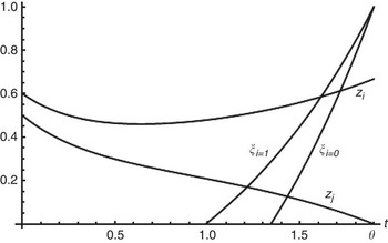
zj (t) continually decreases until j's defeat at time θ ≈ 1.90, where zj (θ) = 0. zi (t) initially decreases until time τ ≈ 0.64, and then increases until time θ when it reaches zi (θ) ≈ 0.67, at which time the war ends in i's victory unless one of the parties has given in to the other's demands rather than continue the fight.
As the war proceeds and i's victory becomes imminent, the best alternative to negotiation ξi (t) also evolves. We assume, furthermore, that discount parameter ri = 1 and that uncertainty is about costs with the range of costs for side  given by:

Since side  is headed for victory at time θ the best alternative for any type i will become positive as t approaches θ. The stronger types i have lower costs and therefore experience a higher payoff from fighting to the finish. For instance, ξi (t) becomes positive at t ≈ 1.0 for i = 1, while i = 0 must wait until t ≈ 1.34 for this to happen. In this example, even the strongest type on side
 has a zero best alternative to negotiation for more than half of the war. The situation is shown in Figure 1.
A victory for Side I

Schedules zj and zi illustrate the evolution of each of the players’ forces over time. If the players fight to the finish, j sees its forces decrease consistently over time until they are entirely depleted at date θ. By contrast, i, the victor can expect an initial decrease in his forces to be followed by growth as he approaches complete victory on the battlefield. Meanwhile, as i approaches victory, fighting to the finish eventually yields a positive expected payoff as the discounted value of the prize exceeds remaining battle costs. In other words, side I's best alternative to a negotiated agreement turns positive to match its expected payoff of a fight to the finish. Side i's best altenative is represented by schedules ξi = 1 for the strongest type on side I and by ξi = 0 for the weakest. The weakest type on side  incurs the highest war costs. The expected value of fighting to the finish therefore turns positive later for type i = 0 than it does for the strongest type i = 1. As illustrated in Figure 1, type i = 1's best alternative, schedule ξi = 1, turns positive at t ≈ 1 while for type i = 0 this does not happen until t ≈ 1.34. Past these dates both ξi = 1 and ξi = 0 grow as remaining battle costs decrease and the discounted value of the prize grows as it becomes increasingly within close reach. As the war ends with j's defeat in battle, schedules ξi = 1 and ξi = 0 converge to the present value of the entire prize, set to 1.
As j is headed for defeat, ξj (t) ≡ 0 at all dates t whatever his type. The range of offers that could be rationally entertained by the two sides should therefore begin to shrink at some time t ∈ (1, 1.34), depending on how much uncertainty has been resolved, until it reduces to the point ξi (θ) = 1 and ξj (θ) = 0 at victory time θ ≈ 1.90. How will war end and what concessions will the rivals make? This is what we find out by examining the equilibria of our bargaining and war game.
War and Bargaining in Equilibrium
Following much of the formal literature we use the perfect Bayesian equilibrium in Markov strategies (MPBE) as solution concept. To investigate the convergence of offers and beliefs and its role in determining the duration of wars, we focus on separating equilibria, which allow the players to learn about each other's types by observing behaviour.Footnote 45
The Findings
The formal analysis of our model is presented in the Appendix and proceeds in three phases. We first obtain the optimal acceptance time for each type, given the two sides’ offers, and the corresponding consistent beliefs. We then characterize optimal offers given consistent beliefs. We finally show the existence of a unique MPBE. The properties of that equilibrium are found to be incompatible with the Principle of Convergence. Offers fall into three classes.
First, the offers that we call ‘convergent’ drive a separation of types and are significant as they grant the other side a positive share that typically exceeds their best alternative to negotiation. For example, an offer schedule that would propose a gradually increasing share of the prize over time, with the increase calibrated to encourage types on the other side to accept an early settlement rather than fight to the bitter end, would be a convergent offer. It would accelerate the screening of types and reduce the duration of the war. Resolution of uncertainty through bargaining would then determine how long the war lasts. An equilibrium involving bilateral convergent offers would, therefore, support the Principle of Convergence. Indeed, convergence requires that offers actually be made and that the resulting screening process ensures that the players learn from their opponent's response to their offers.
Secondly, at the boundary of the set of convergent offers lies the set we simply refer to as ‘boundary offers’. Such offers may be either separating or significant, but they cannot have both features. If a boundary offer drives a separation of types it must match the other side's best alternative to a negotiated settlement. As long as fighting to the finish is more costly than the discounted value of the prize enjoyed in perpetuity, the best alternative to a negotiated settlement is nil, the boundary offer is also nil and types are revealed by the simple passage of time for those unwilling to continue the fight. If, instead, a boundary offer is significant this is because the other side is nearing victory and enjoys a positive best alternative to negotiation. This significant offer then has the effect of hiding the types of the losing side that makes it and, therefore, fails to be separating.
Thirdly and lastly, we define the set of offers that are unacceptable. For example, an offer that falls below the other side's best alternative to negotiation would never be accepted by a rational player and, therefore, joins the set of unacceptable offers. But there are other types of offers that would never be rationally accepted. It turns out that offers that increase too fast or that involve discontinuities are also unacceptable, because they prompt the other side to wait with certainty for a while.
On the way to building the proof of our main theorem, we obtain two substantive results. The first result (Lemma 8 in the Appendix) asserts that a convergent offer can always be profitably reduced by the side that makes it. The intuition behind this result is as follows: a substantial offer accelerates the screening of the other side's type by prompting each type on the other side to end the war sooner than it would by relying on its resilience alone. Thus, accepting the substantial offer reduces war costs by shortening the fight. But it turns out that the reduced war costs for the side making the compromise offer do not compensate for the receiving of a reduced share of the prize and this speaks in favour of reducing the size of the offer. Indeed, the compromising side could, with some probability, be facing a type on the other side who would have surrendered right away. And the expected gain from reduced war costs does not match the expected loss from giving away part of the prize to a possibly weak type on the other side. The second result (Lemma 9) implies that optimal offers can never match, meaning that there is always a spread between the two sides’ proposals, unless and until one side reaches victory. As a result, in this continuous-time framework, it is not rational to reach an early compromise without fighting. These two first results lead to our central theorem that establishes the existence of an equilibrium that must involve boundary offers on each side.
In sum, equilibrium behaviour in our model involves standing firm and making no concession for most of the war. In fact, if there is stalemate, optimal behaviour dictates that neither side ever makes any concession despite the ongoing convergence of beliefs. As a result, the game turns into a pure war of attrition despite the possibility of negotiation. The Principle of Convergence is clearly not involved in determining such wars’ duration. Instead, these wars will last until one side surrenders to the other giving up the entire prize. If one side is expected to win, no concessions are made until the winner's expected utility from a fight to the finish is positive. Only then will the losing side make offers that affect the duration of the war by prompting the winning side to accept a settlement rather than fight to the bitter end. Thus, for much of these wars neither side concedes anything to the other and duration is determined by the resilience of the types on each side, not by screening as the Principle of Convergence suggests. For this initial phase of the war, the Principle of Convergence is not involved in determining duration. When victory becomes imminent, then screening by the losing side does affect war duration but it does so through a process that is arguably very different from the one that is typically envisaged by the convergence principle. In a discrete-time model with bilateral uncertainty, the workings of the Principle of Convergence would dictate a process of alternating offers and counteroffers designed to satisfy the weakest type still standing on each side. And the process would begin with the start of hostilities. In our model, when victory becomes imminent, the losing side actually hides its type by ruling out surrender in favour of extending offers that could prompt the weaker types on the winning side to settle rather than fight. The intent for the losing side is to try to save something for himself now that the winner has revealed herself to be resilient enough to prefer a fight to the finish. The objective is not to reveal the winner's type but to salvage what might be possible from the ruins of defeat.
We now turn to a numerical example to illustrate these findings.
A Numerical Example
Consider again our example in which  is the winning side. Also assume that utilities are given by ui (x) = x. Finally, assume symmetric parameters for side J, except that j's costs are given by cj(zi, zj) = (3−j)(zi + zj). Each type
 has an expected payoff
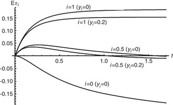
 defined by Equation 4 given the two sides’ respective offers and beliefs. We illustrate expected payoffs for the three types I = 0, 0.5 and 1, given side J's optimal offer yj, which we will describe in Figure 3 below. We consider two possible offers, yi ≡ 0 and yi ≡ 0.20, by side
 and trace out, in Figure 2, the expected payoff to the three types of waiting time t to accept side J's outstanding offer. Expected payoffs on the vertical axis are measured against waiting times on the horizontal t axis.
Expected payoffs

Figure 2 illustrates two things: first, although  is the winning side, the weaker individuals on side
 will prefer to give in to side J's offer before victory rather than fight to the finish. For example, type i = 0 experiences negative expected payoffs from the start and so would be better off accepting side J's standing offer at time t = 0, which is yj (0) = 0. This is, of course, an extreme case and expected payoff schedules shift continuously as i becomes more resilient. Type i = 0.5 would give in to the extreme demand yj = 0 by side J around t = 0.25, assuming i made no concession, and weaker types i ∈ [0, 0.5] would give in to yj = 0 sooner. Indeed, Figure 2 shows that, given yi ≡ 0, type i = 0.5's expected payoff from waiting time t to accept J's standing offer reaches a maximum around t = 0.25. Type i = 1, the most resilient, actually finds it optimal to fight to the finish when offering yi ≡ 0, and only until offers match when offering yi ≡ 0.20.
Secondly, given J's optimal offer yj, no type on side  has any interest in extending a positive offer yi to J. Observe that, given type, the expected payoff associated to the offer yi ≡ 0.20 is always lower than the expected payoff associated to yi ≡ 0. Given J's optimal offer, all types on side
 strictly prefer to stand firm on initial demands as their expected payoffs shrink with any concession made to the other side. Figure 2 shows the situation at the onset of the war. As time passes, types i ∈ [0, φi(t)) are screened out and all expected payoffs for i ∈ [φi(t), 1) shift down and to the left, with i = φi(t) taking the place of i = 0 and seeing the expected payoff decrease from that time on. We now illustrate optimal behaviour.
As seen above, side  ultimately wins. As a result, if war drags on up to time t ≈ 1, active types see their best alternative to negotiation turn positive and side J starts optimally making concessions. But until then side J makes no concession whatsoever. With side I's victory approaching, side J attempts to salvage some of the prize for himself by making an optimal offer that must satisfy
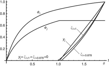
 , which involves a concession to some of the active types i ≥ φi(t) on side I. While the winding down of the war comes with concessions from side J, uncertainty about i's type narrows. This can be seen by observing φi as it changes over time. Figure 3 plots φi, φj and equilibrium offer yj together with the best alternatives to negotiations ξi for types i = 0.878 and i = 1. Equilibrium offer yi ≡ 0 for side I is not shown but is implicit in the picture.
Beliefs and optimal offers

Optimal offer yj starts out being identically nil, just as all ξi's are, but turns positive as victory for side I is looming. At time t* ≈ 1.03, type i = φi(t*) ≈ 0.878 accepts what is still a nil offer yj(t*) = 0. But immediately after t*, optimal offer yj becomes positive. yj initially lies below the strongest type's (i = 1) best alternative ξi = 1 but somewhat above ξi = 0.878. So, for t > t* there is a range of types i ∈ (0.878, 1) for whom the optimal yj(t) is strictly above their best alternative ξi(t) and is therefore a small concession. Offer yj increases at a rate that results in the constant consistent belief φj, as all remaining active types j adamantly refuse to accept side I ‘s optimal offer yi ≡ 0.Footnote 46 Offer yj is, therefore, a boundary offer as it is either nil or prevents the separation of types on side J.
The fact that side J's optimal offer increases over time leads the stronger types on side I to wait before accepting, although the current offer exceeds their current best alternative to negotiation. Recall that side I's acceptance time is determined by maximizing its expected payoff from waiting to accept J's optimal offer as illustrated in Figure 2. Expecting better offers to come their way, active types on side I will optimize their expected payoffs by fighting longer, delaying acceptance, and after time t*, active types i will accept deals that are strictly better than fighting to the finish. Of course, the stronger types will only accept the more generous offers. For example, types i close to 1 will only accept an offer that is close to the entire prize. And the strongest type on side  , i = 1, will fight to the finish for the entire prize.
Discussion
The uncompromising bargaining behaviour that emerges from our results persists as each side gathers more information about the type he is facing. Beliefs converge in our model but it is only the imminent victory of one side that prompts significant offers by the losing side, and these offers are a little better than those that the impending winner can guarantee himself by fighting to the finish. Our model, therefore, predicts that the winning side could well stop short of a complete military victory and accept the loser's attempt to limit the damage. The victor would then agree to a little less than the entire prize having already achieved most of his objectives. For example, the United States and its allies stopped short of marching into Baghdad in the First Persian Gulf War, preferring instead to withdraw the troops having achieved the liberation of Kuwait and the clear defeat of Iraqi troops in the Desert Shield ground offensive. By bringing the troops home, leaving Saddam to extol Iraqi courage in the ‘Battle of Battles (Um Al-Ma'arik), where Iraq stood fast against the invasion, maintaining its sovereignty and political system’,Footnote 47 the United States was arguably accepting less than complete victory, having achieved most of its objectives.
By contrast, if the war evolves to a stalemate, the model predicts that one side will eventually cave in and accept the other side's position, although this may take a very long time. The Korean War is a case in point. As Carter Malkasian points out, General Ridgeway, commander of the Eighth Army, and Peng Dehuai, commander of the Chinese People's Volunteers, ‘both envisaged a protracted war, seeking to compel concessions from the opponent’.Footnote 48 Following what Andrew Birtle describes as the three years of stalemate, North Korea conceded the right to voluntary repatriation of those who had escaped the communist regime, after conceding the 1951 line of contact between the warring armies as the cease fire line.Footnote 49 According to Malkasian, within the context of limited American war aims designed to avoid an escalation to ‘a general war’ between the United States and the Soviet Union or the People's Republic of China, `the stalemate in Korea ended with North Korea's full back down’.Footnote 50
Following Allan Stam, we model war as an effort by both sides to coerce the other to adopt his point of view.Footnote 51 What our model predicts, however, is that if war is a bargaining process it is one that is indeed what Thomas Schelling would describe as ‘dirty, extortionate and often quite reluctant’.Footnote 52 The screening implied by our no-concession result stands in stark contrast with the screening process that underlies the Principle of Convergence. Convergence in Filson and Werner, in Slantchev or in Powell is achieved by calibrating offers in each decision period to the weakest type still standing.Footnote 53 As information becomes more complete or decisions become more frequent that process converges to a true compromise offer that is beneficial to both sides. By contrast, we have shown that if both players are allowed to make offers and accept them at the time of their choosing they do not make any meaningful compromise, at least until the imminent victory of one side. Instead, they both demand that the other accept the minimum it can guarantee itself by continuing to fight, which means complete surrender for much of the war. Most importantly, this divergence persists as uncertainty vanishes and regardless of the identity of the expected winner.
Our rivals are out to identify the weakest of the two sides rather than the weakest among the opponent's types. If one were to make a concession, then all types on the other side would accept sooner. But if the side to offer compromise happens to be stronger than the other, it forgoes the opportunity to see its opponent just take a minimal offer. With a compromise offer on the table, war might be shorter and, therefore, less costly. But these expected savings do not compensate for the benefit of having a weak type on the other side decide to make do with his best alternative to negotiation. In equilibrium, our rivals implement passive screening for much of the war, offering no concession and hoping that the other side will give in before they do. Only when it is facing imminent defeat does one side begin making significant offers in order to cut short its losses, while adamantly refusing to capitulate. According to our model, wars erupt and endure because the rivals do not rationally seek compromise until the impending victory of one side. This is in stark contrast with the idea that wars are fought to inform on the terms of the bargain that each is willing to accept.
The attrition behaviour that our model predicts can be tested for empirically. Indeed, the failure of both parties to offer concessions in equilibrium implies, technically, that the likelihood that each side will give in increases as the flow costs of war incurred by the other side increase (see formula (A4) in Appendix). Langlois and Langlois test this relationship.Footnote 54 Specifically, the attrition behaviour that our model anticipates involves weighing the expected costs of war against the chances that the other side will give in to one's demands. The lower the believed likelihood that the opponent will give in, the lower the flow costs one should be willing to bear for the same prize. If beliefs are an accurate prediction of rational behaviour, this implies that higher war flow costs suffered by one side are associated to a higher probability of surrender or concession by the other. This is not a statement about battle deaths or military capabilities as they affect the course of the war. Rather it is a statement about a state's willingness to commit resources to the war effort given the other side's perceived willingness to fight on. To test for attrition behaviour we used the proportion of a state's population engaged in military activities, a comprehensive measure of a state's investment in war, as a predictor of the other side's willingness to give in. Our analysis of seventy-two interstate wars that have occurred between 1823 and 1990 reveals that, once traditional drivers of duration such as battle deaths, capabilities and terrain are accounted for, the proportion of a state's population in the military positively, and significantly, affects the other side's willingness to give in. Therefore, we conclude that the attrition behaviour predicted by our model can help to explain the duration of interstate wars.
Conclusion
Convergence in war and bargaining models describes a screening process, in which fighting informs, and concessions are calibrated to prompt the separation of types. The convergence of beliefs results in a convergence of offers. To investigate the impact of the discrete-time modelling assumptions made by these models, we have constructed a war and bargaining model that allows the rivals to bargain freely while fighting in the time continuum. Uncertainty and bargaining are bilateral and the rivals can make offers and counteroffers at the time of their choosing. In our model warfare is an ongoing process that allows for stalemate as well as victory by one side or the other. In this context we find that, in equilibrium, the rivals will adopt uncompromising bargaining positions, preferring to fight it out in the hope that the other side will give in first.
Uncompromising bargaining behaviour prevails as long as there is a chance that the other side will surrender under the continued pressure of battle costs. Only when defeat is imminent will the losing side offer small one-sided concessions. In our model, only the dynamic progression of battle towards one side's ultimate demise prompts the loser to sue for peace and offer concessions. As long as defeat is remote or uncertain, the potential for the opponent's surrender drives the rivals to adopt uncompromising positions despite the increasing likelihood that their opponent is resilient. The progress of battle informs on the resilience of the rivals but it does not bring them to the bargaining table. In equilibrium, the convergence of beliefs does not lead to a convergence of settlement offers. The active screening that is at the core of the process of convergence does not take place, and the Principle of Convergence does not hold.
Mathematical Appendix
If i believes that, at time t, all types j ∈ [0, φj (t)) have been screened out then only those types in the segment [φj (t), 1] remain active. If we further write

then φj(s|t) represents i's beliefs, conditional on reaching time t, about what segment of [φj(t), 1] will have been screened out after a further delay s. Using more generally the notation ‘s|t’ for all variables evaluated at (t + s), conditional on reaching time t, one can rewrite i's expected payoff defined in Equation 4 for waiting time (t + s), with s ≥ 0, as


where πi (yj (s|t), s|t) is as in Equation 1, but involves only the developments from time t on, and  is the total cost ‘sunk’ in the war effort by time t.
 is i's expected payoff from time t on and it has the very same structure as
 . Sequential rationality thus requires the maximizing of
 at each time t over s and offer function yi (.|t) given beliefs. This is clearly equivalent to optimization from the very start by Equation A2 as long as φj(t) < 1.
For simplicity of exposition we state and prove all claims with initial t = 0. In particular, one has φj(0|t) = 0 just like φj(0) = 0, but this assumes that current belief φj(t) at time t is accounted for by Equation A2. The general case only requires the burdensome notation ‘s|t’ in all statements and proofs below.
A belief–strategy profile is called consistent if beliefs are consistent with strategies according to Bayes’ Law. Since offer functions yi and yj are assumed right-differentiable and piecewise C1, we find that consistent beliefs inherit the same properties. If φi is continuous and increasing at time t this means that i = φi(t) is the single type i who accepts optimally j's offer yj(t) at time t. A discontinuity Δφi(t) = φi(t)−φi(t −) > 0 could instead mean that a segment of types [φI(t −), φi(t)] accepts yj(t) at time t. But Δφi(t) > 0 could also result from signalling, if side  makes an offer yi at time t that no type in [φi(t −), φi(t)) could make.Footnote 55 However, we will find that all active types i have the same optimal offer yi and that such signalling is suboptimal. So we focus on acceptance as the updating instrument.
We state that offers ‘match’ at time t if yi(t) + yj(t) = 1 but yi(s) + yj(s) < 1 for all s < t. When offers match the two sides agree on the split and the game ends.Footnote 56 Offers are assumed defined for all times even if they match before the game ends.
For simplicity of exposition, we also assume that ui(x) = x, although all proofs are easily extendable to the case where ui is a strictly increasing C1 function.Footnote 57 We denote by δ(s) = 1−yi(s)−yj(s) the spread between the two sides’ offers. Also for simplicity we denote by  the quantity
 , and similarly for
 and
 .
We first characterize optimal acceptance times and the resulting consistent beliefs.
Definition 1 A (belief–strategy) profile is separating for side  in an interval Ω = [0,t) if side J's consistent belief φi is continuously increasing within that interval.
Lemma 1 If the profile is separating for side  in Ω = [0, t) then, for all s ∈ Ω where offers are differentiable, consistent beliefs must satisfy:


Proof. Since φj is a distribution function it is differentiable almost everywhere (a.e.). And since offers are piecewise C1, i accepts optimally at time s ∈ (0, t) only if the first order condition

holds (a.e). Simplifying Equation A5 yields:

By consistency of beliefs, Equation A6 must hold at s for the single type i = φi(s). Since λi(s) is piecewise continuous, belief φj is piecewise C1 (i.e. it inherits the properties of offers). And Equation A4 also holds at s = 0, in the sense of the right-hand side derivative.
By Equation A4, the inequality  is necessary for φj to represent side I's beliefs. Clearly, the sign of λi is determined by yj. But the condition
 within Ω = [0, t) can occur and implies constant beliefs φj (s) ≡ 0. However, the condition
 obtains if yj increases sufficiently fast within Ω. In that case, Equation A4 cannot hold but we will show that consistent beliefs must then remain constant. Consistent beliefs will also remain constant when none of the types can rationally accept within the given interval. This occurs if offer yj(s) falls below the best alternative ξi(s) to negotiation for all active types i ≥ φi(s) in Ω. We therefore make:
Definition 2 Given consistent beliefs, an offer yi is called in Ω = [0, t)
(1) ‘acceptable’ if it satisfies in all Ω

(2) ‘convergent’ if both inequalities in Equation A7 are strict in all Ω;
(3) ‘boundary’’ if Equation A7 holds with at least one equality in all Ω;
(4) ‘unacceptable’ if at least one of the inequalities in Equation A7 fails in all Ω.
A profile is called ‘acceptable’ if both sides’ offers are acceptable.
LEMMA 2 If yi is unacceptable in Ω = [0, t), then side I's consistent belief φj must be constant in Ω. Moreover, unless offer yj is such that  , side J's consistent belief φi must also be constant in Ω.
Proof. If  then j = φj(s) cannot optimally accept at s. And if
 , then
 (in Equation A5 written for j), and j cannot optimally accept at s.Footnote 58 In either case, no active j can accept and consistent beliefs φj (s) can only be constant in Ω. If yj is also unacceptable then φ i(s) ≡ 0 by a symmetric argument. And if yj is acceptable but such that
 , then (with
 since φj(s) ≡ 0)

at s such that i = φi (s). So, this i cannot accept optimally at that time s and consistent belief φi can only be constant in Ω.Footnote 59
To complete our description of consistent beliefs, we consider discontinuities in offers.
LEMMA 3 Assume that Δyi (t) = yi(t)−yi(t −) > 0. Then side I's consistent belief φj must be constant in some Ω = [t′, t). Moreover, unless offer yj is such that  in Ω, side J's consistent belief φi must also be constant in Ω.
Proof. Let Δφi (t) = φi (t)−φi (t −) ≥ 0 and let j = φj (s) be the type that accepts optimally at s ∈ Ω. This requires that  . But
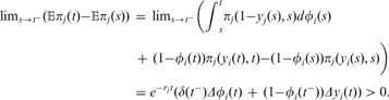
So, if t′ < t is sufficiently close to t, all  and no j can accept optimally in Ω. The same arguments as in Lemma 2 then apply.Footnote 60
So, a positive jump in offer yi at t creates an interval before t where yi is also ‘unacceptable’ with the very same consequences on consistent beliefs. Therefore, we can extend the definition of unacceptable offer to the case of a discontinuous jump at t, within an adequate interval Ω = [t′, t). A negative drop Δyi (t) < 0 can be characterized similarly.Footnote 61 In fact, it requires an interval after t where the offer is unacceptable in order for beliefs to be consistent. But this last result will not be needed in our proofs, since we will only consider drops from a minimum acceptable offer that are trivially unacceptable.
We now have a clearer picture of consistent beliefs: unacceptable offers yield constant beliefs within a corresponding interval. And those with a discontinuous jump have a similar effect. Since we will obtain an equilibrium in continuous offers, we initially focus on the continuous case and will eventually show that unacceptable, including discontinuous, offers are suboptimal
LEMMA 4 Given that offers yi and yj are continuous and do not match in the interval [0, t), there exists a unique pair of consistent beliefs  and
 . Moreover, beliefs depend continuously on offers.Footnote 62
Proof. We can rewrite Equation A4 in view of Lemmata 2 and 3:


and symmetrically for  . Clearly, fi and fj are piecewise continuous in s. And they have bounded partial derivatives in φi and φj. Given initial φi(0) = φj(0) = 0 this first order system of differential equations has a unique solution by Picard's Theorem.Footnote 63 The solution satisfies

This clearly defines a distribution function and, therefore, beliefs. Moreover φj in Equation A11 fits the conditions of Lemmata 1, 2 and 3, and, therefore, defines the unique consistent beliefs. Finally,  and
 depend continuously on offers and so do φi and φj.Footnote 64
We now restrict our attention to continuous acceptable profiles and obtain necessary conditions of optimality within that set. We still denote victory time (for either side) by θ ≤ ∞. The case θ = ∞ means battlefield stalemate.
LEMMA 5 If side J expects to win the war at time θ, or if θ = ∞, then the minimum acceptable offer  for side
 is
 .
Proof. Since side I cannot win ξi (t) ≡ 0 for all i, and since  yields λi (t) > 0 for all i and t, it is acceptable. Since no offer can be negative this is the minimum.
LEMMA 6 If side  expects to lose the war at time θ < ∞then, given any continuous offer yj, there exists a unique minimum (continuous acceptable) offer
 for side

Proof. For any continuous yi, let  be the unique consistent beliefs obtained in Lemma 4. Now let
 be defined for all
 by:

If we let  then
 (the topological closure of
 ).
 , having uniformly bounded variations, is equicontinuous. And since [0, θ] is compact, by Ascoli's Theorem,Footnote 65
 is compact. And it is clearly convex. Moreover, both
 and
 are continuous operators and so is the composite

So, the operator  is compact and convex. By Schauder's Theorem, it has a fixed point
 .Footnote 66 Wherever positive,
 must, therefore, satisfy, with
 as consistent belief

which is the solution of  together with
 . Moreover,

since  for all τ ≥ s. So
 is indeed acceptable.
We now show that  is the minimum continuous acceptable offer in [0, θ]. Whenever
 , this is trivial. Otherwise, for any
 the necessary conditions
 and yi (θ) = 1 for yi to be acceptable yield, by integration, for all s ∈[0, θ]:

If, in addition,  for all such s, then one easily verifies that

Since this yields  , we must have by Equations A13 and A15,
 . So, no acceptable yi (s) can be strictly less than
 . Since this holds for all s ∈ [0, θ],
 must be unique.Footnote 67
To obtain the No-Concession Result central to all our findings we need:
Lemma 7 For any (continuous acceptable) profile in an interval Ω = [0, t) and for all active types  and for all s ∈ Ω:

Proof. Since  in Equation A5 must be piecewise continuous, we may write

Inserting Equation A4 into Equation A17 and simplifying yields Equation A16.Footnote 68
Lemma 8 (No Concession): If yi is a best-reply offer (for all active types i) to yj in a continuous acceptable profile then it must be the minimum  .
Proof. First assume that offer yi is convergent in some interval denoted Ω = [0, t) and let ti ≥ 0 be such that type i = φi (ti) accepts optimally at time ti ∈ Ω. Also denote by Li[yi] the integrand in Equation A16 evaluated at s = ti. Type i seeks an offer yi that maximizes Li[yi].Footnote 69 Now, for all s ∈ Ω, let η(s) = s−t, and

By continuity, for h > 0 small enough,  in Ω.Footnote 70 So,
 is a continuous acceptable offer in Ω. Furthermore,

Since the last term is nil by i = φi (ti),Footnote 71 we only need to show that the integrand is negative at h = 0 so that  is strictly better than yi for h > 0 small enough. We have


Moreover, omitting all time arguments for simplicity,
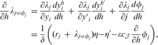

Clearly, both above quantities are bounded in Ω and we can letFootnote 72


Replacing in Equation A21 and Equation A22 yields, since η ≤ 0,

It follows that, with 0 < δ* ≤ δ(s),  and
 on Ω,



for t > 0 small enough (with all quantities evaluated at h = 0).
So,  and
 for h > 0 small enough is a strictly better continuous acceptable offer for all types i who accept in Ω. Moreover, if a convergent yi is best for some active types who do not accept in Ω, let i* ≥ φi(t) be the infimum of all such types. If any type i ≥ i*, makes a convergent offer yi in Ω it ‘signals out’ all types i < i* and consistent belief φi must be updated so that we may now let i* = φi(0) = 0. Since belief φj is unaffected, the offer yi is still convergent in Ω. But, by the above argument, yi cannot be optimal.Footnote 73
Secondly, assume instead that yi is a boundary offer other than  in some interval Ω. If the current time (denoted 0) is close enough to θ this requires
 , with resulting
 and, therefore, φi ≡ 0 in Ω. So, yi is strictly increasing. Without loss of generality we can assume that yi(t) = 1 at time t < θ, otherwise it would be equal to
 . Solving
 with yi(t) = 1 yields, for all s ∈ Ω,

with consistent beliefs  and φi ≡ 0 in Ω. It follows that

as long as  since
 . But

since  . It follows that an increase in t results in a uniform decrease in yi and a corresponding uniform decrease in φj while φi remains constant. Therefore,

and a decreased boundary yi is strictly better for all active types i.Footnote 74
The only offer that cannot be improved upon and is therefore the only possible best reply for all active types is the minimum  .
We have only obtained necessary conditions for best-reply offers within the set of continuous acceptable profiles. In the next result we show that there exists an equilibrium within that set and characterize it. We then show that it is an MPBE of the game without the restriction to continuous acceptable offers.
Lemma 9 Within the set of continuous acceptable profiles there exists a unique MPBE and it is made up of the minimum acceptable offers  and
 .
Proof. If there is no victory time θ < ∞, we pick an arbitrary (large but finite) θ and impose the restriction that yi(s) ≡ yi(θ) for all s ≥ θ. Since decreasing acceptable offers are convergent and cannot be best replies by Lemma 8, we can limit our search for an optimum to the set  of non-decreasing continuous acceptable offers. Since
 is a closed subset of
 (in Lemma 6) it is compact. Since the operator Li[yi] is continuous in yi it must reach a maximum over
 . If side
 is not losing, this maximizand can only be the (unique) minimum acceptable
 that is common to all active types i. If side
 is losing, then side
 is winnint and
 . But there is a unique maximizand
 of Li[yi] in response to
 by Lemma 6 for all active types i. And if there is a stalemate
 is the optimum for any finite θ and, therefore, for all times.
We denote by  the pair
 formed by the above minima together with consistent beliefs
 .Footnote 75 We now show that
 is in fact an unrestricted MPBE.
Theorem The profile  of Lemma 9 forms an MPBE of the game.
Proof. First, observe that a discontinuous jump in offer is unacceptable in some interval Ω by Lemma 3. And a discontinuous drop from the minimum acceptable offer can only be unacceptable. So, we only need to show that unacceptable offers are suboptimal. Consider an interval [0, t) where yi is unacceptable in response to  . By Lemma 2, consistent belief φj becomes constant (equal to 0) in Ω and the expected payoff for any active type i reduces to
 in Ω. If we denote by
 the expected payoff under
 , we have two cases for
 :
(1)
in Ω. In that case . So, there can be no improvement for any type i in switching to yi;(2)
and all λi > 0. In that case, one easily verifies that for all s ∈ Ω:
 in Ω. In that case
 . So, there can be no improvement for any type i in switching to yi;
 and all λi > 0. In that case, one easily verifies that for all s ∈ Ω:

But this is equivalent to  . So, all active types i's expected payoffs are uniformly decreased in all Ω by the switch to yi. Moreover, all conditional expected payoffs
 in Equation A3 are unchanged since yi is unchanged after time t. So, all expected payoffs are uniformly decreased for all times under the switch. In particular, optimal expected payoffs are uniformly decreased. And this holds for any t.
 .
 reflects the fact that φj can be discontinuous. At discontinuities dφj(s) is a mass with magnitude equal to the size of the jump.
 for all t ≥ θ since, also by convention, xi ≡ 1−yi(s) ≡ yj(t) for all t ≥ s ≥ θ.
 discussed in the Appendix (Definition 2).
 's belief just before that offer, belief jumps to φi(t) = i* at time t.
 and would be a net loss for any i who could accept 1−yj(t) instead.
 by
 in all formulae.
 allows an increasing belief φi while offer yi is unacceptable. The consequences for belief φi are only given for the completeness of Lemma 4. But only the consequences for belief φj are necessary in the Main Theorem at the end.
 . But the jump Δφj(t) > 0 would be incompatible with an acceptable profile starting at t. Proofs of these statements are available from the authors upon request.
 and
 are continuous in the topology of uniform convergence (or any weaker topology).
 . If offers match at time t, and then
 becomes infinite and φj(t) = 1 provided
 . If beliefs need to be defined for s ≥ t we simply set them as the constant φj(s) ≡ φj(t).
 and yj match at some t < θ. In that case, belief φi may (or may not) reach the value 1 in the interval [t, θ]. Also note that yj need not be acceptable in this argument.
 , the integrand in Equation A7 is nil and
 where yj(θ) is the outcome of war or the agreed upon bargain at time θ.
 , then
 has no effect on
 , which remains nil.
 can obtained by differentiating the identity i = φi(ti).