1 Introduction
Industrial applications and real-life cases often involve suspensions of non-spherical particles, of either regular or irregular shapes. Prolate (needle-like) spheroids can be used to describe milled biomass particles, fibrous suspensions and submarine hulls. On the other hand, oblate (disc-like) particles can be used as an approximation to represent red blood cells. El Khoury, Andersson & Pettersen (Reference El Khoury, Andersson and Pettersen2010, Reference El Khoury, Andersson and Pettersen2012) performed direct numerical simulations (DNS) with the flow perpendicular to the symmetry axis of the spheroid and investigated the wakes behind a prolate spheroid of ratio 6 : 1. Hölzer & Sommerfeld (Reference Hölzer and Sommerfeld2009) and Zastawny et al. (Reference Zastawny, Mallouppas, Zhao and Van Wachem2012) investigated different non-spherical particles at different flow incident angles at different Reynolds numbers (
 $\mathit{Re}$
), albeit limited mainly to the steady flow regime. Very recently, Ouchene et al. (Reference Ouchene, Khalij, Arcen and Tanière2016) proposed force correlations for prolate spheroids up to an aspect ratio of 32, again limited to steady flows with
 $\mathit{Re}\leqslant 240$
. They reported an interesting finding that the drag coefficient
 $C_{D}$
of the prolate spheroids follows a sine-squared interpolation between its extreme
 $C_{D}$
values for
 $\mathit{Re}\leqslant 240$
for the reported aspect ratios. In this paper, we investigate this phenomenon more deeply and to higher
 $\mathit{Re}$
.
Some authors define the Reynolds number
 $\mathit{Re}_{d}$
based on the minimum thickness of the particle
 $d_{min}$
. For this work, the Reynolds number is defined as
 $\mathit{Re}=|\boldsymbol{u}_{\infty }|d_{eq}/\unicode[STIX]{x1D708}$
, where
 $\boldsymbol{u}_{\infty }$
is the uniform inlet velocity,
 $\unicode[STIX]{x1D708}$
is the kinematic viscosity of the fluid and
 $d_{eq}$
is the diameter of the volume-equivalent sphere given by
 $d_{eq}=(6V_{p}/\unicode[STIX]{x03C0})^{1/3}$
, with
 $V_{p}$
being the particle volume. The drag coefficient is defined as
 $C_{D}=|\boldsymbol{F}_{D}|/((1/2)\unicode[STIX]{x1D70C}|\boldsymbol{u}_{\infty }|^{2}(\unicode[STIX]{x03C0}/4)d_{eq}^{2})$
. Here,
 $\boldsymbol{F}_{D}$
is the drag force acting on the particle and
 $\unicode[STIX]{x1D70C}$
is the fluid density. For any particle in the Stokes regime (Happel & Brenner Reference Happel and Brenner1983), based on linearity of the Stokes equations, the drag coefficient at different incident angles
 $\unicode[STIX]{x1D719}$
interpolates as
 $$\begin{eqnarray}\displaystyle & C_{D,\unicode[STIX]{x1D719}}=C_{D,\unicode[STIX]{x1D719}=0^{\circ }}+(C_{D,\unicode[STIX]{x1D719}=90^{\circ }}-C_{D,\unicode[STIX]{x1D719}=0^{\circ }})\sin ^{2}\unicode[STIX]{x1D719}. & \displaystyle\end{eqnarray}$$
Here, the subscript
 $\unicode[STIX]{x1D719}$
implies the value at that particular incident angle
 $\unicode[STIX]{x1D719}$
.
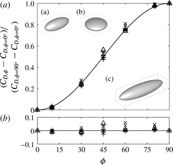
(a) The normalized drag coefficient
 $(C_{D,\unicode[STIX]{x1D719}}-C_{D,\unicode[STIX]{x1D719}=0^{\circ }})/(C_{D,\unicode[STIX]{x1D719}=90^{\circ }}-C_{D,\unicode[STIX]{x1D719}=0^{\circ }})$
plotted against the incident angle
 $\unicode[STIX]{x1D719}$
. The solid line indicates
 $\sin ^{2}\unicode[STIX]{x1D719}$
. Data include (a) a prolate spheroid (
 $+$
) and (b) an oblate spheroid (
 $\times$
), both of aspect ratio
 $5/2$
, both for
 $\mathit{Re}=0.1$
, 10, 100, 1000 and 2000, and (c) a prolate spheroid of aspect ratio 4 (▵) for
 $\mathit{Re}=2000$
. Averaged
 $C_{D}$
values are used for cases with vortex shedding occurring at high
 $\mathit{Re}$
. (b) The difference between the normalized drag coefficient and
 $\sin ^{2}\unicode[STIX]{x1D719}$
.

To motivate the reader, the drag on different spheroids is tested up to
 $\mathit{Re}=2000$
and the mean values of
 $C_{D}$
are plotted in figure 1. Surprisingly, the investigated particles follow sine-squared interpolation very well for both steady and unsteady regimes, even for
 $\mathit{Re}$
as high as 2000. This interesting phenomenon appears to be similar to the Stokes regime prediction (1.1), as mentioned by Ouchene et al. (Reference Ouchene, Khalij, Arcen and Tanière2016). We investigated the phenomenon in detail and found a plausible reason and also the limitations of the sine-squared behaviour. Our findings at high
 $\mathit{Re}$
, in combination with observations of Ouchene et al. (Reference Ouchene, Khalij, Arcen and Tanière2016) for prolate spheroids up to aspect ratio 32, extend the validity of the drag law to both high-aspect-ratio prolate spheroids and high
 $\mathit{Re}$
. This implies that, in many situations, the mean drag coefficient at any incident angle
 $C_{D,\unicode[STIX]{x1D719}}$
for a given
 $\mathit{Re}$
can be obtained by just knowing two values,
 $C_{D,\unicode[STIX]{x1D719}=0^{\circ }}$
and
 $C_{D,\unicode[STIX]{x1D719}=90^{\circ }}$
.
2 Numerical method
2.1 Lattice Boltzmann method
The fluid flow is simulated using a D3Q19 multi-relaxation-time (MRT) lattice Boltzmann method (LBM) (d’Humières et al.
Reference d’Humières, Ginzburg, Krafczyk, Lallemand and Luo2002). The MRT-LBM scheme solves the evolution of the particle distribution function
 $|\,f\rangle$
,
 $$\begin{eqnarray}|\,f(\boldsymbol{r}+\boldsymbol{e}_{\unicode[STIX]{x1D6FC}}\unicode[STIX]{x0394}t,t+\unicode[STIX]{x0394}t)\rangle =|\,f(\boldsymbol{r},t)\rangle -\unicode[STIX]{x1D648}^{-1}\hat{\unicode[STIX]{x1D64E}}(|m(\boldsymbol{r},t)\rangle -|m^{(eq)}(\boldsymbol{r},t)\rangle ),\end{eqnarray}$$
for position
 $\boldsymbol{r}$
with discrete velocities
 $\boldsymbol{e}_{\unicode[STIX]{x1D6FC}}$
in directions
 $\unicode[STIX]{x1D6FC}=1,2,\ldots ,19$
. Here,
 $\unicode[STIX]{x1D648}$
is a
 $19\times 19$
transformation matrix used to transform
 $|\,f\rangle$
from velocity space to moment space
 $|m\rangle$
, with
 $|m\rangle =\unicode[STIX]{x1D648}\boldsymbol{\cdot }|\,f\rangle$
; the ket vector
 $|\cdot \rangle$
implies a column vector. The relaxation matrix
 $\hat{\unicode[STIX]{x1D64E}}=\unicode[STIX]{x1D648}\boldsymbol{\cdot }\unicode[STIX]{x1D64E}\boldsymbol{\cdot }\unicode[STIX]{x1D648}^{-1}$
is a
 $19\times 19$
diagonal matrix. The relaxation matrix
 $\hat{\unicode[STIX]{x1D64E}}$
utilizes different optimally chosen relaxation rates for different moments, thereby providing better stability compared with the single-relaxation-time LBM scheme (d’Humières et al.
Reference d’Humières, Ginzburg, Krafczyk, Lallemand and Luo2002). The matrices
 $\unicode[STIX]{x1D648}$
and
 $\hat{\unicode[STIX]{x1D64E}}$
are similar to those of Huang et al. (Reference Huang, Yang, Krafczyk and Lu2012). The kinematic viscosity of the fluid is set by the relaxation time
 $\unicode[STIX]{x1D70F}$
as
 $\unicode[STIX]{x1D708}=c_{s}^{2}(\unicode[STIX]{x1D70F}-1/2)\unicode[STIX]{x0394}t$
and the pressure
 $p$
is related to the density by
 $p=\unicode[STIX]{x1D70C}c_{s}^{2}$
. Uniform velocity in the
 $z$
direction is prescribed at the inlet boundary based on the work of Hecht & Harting (Reference Hecht and Harting2010). The sidewalls are prescribed with free-slip boundaries rather than periodic boundary conditions, which could cause the flow to deflect either up or down based on the inclination of the non-spherical particle (Hölzer & Sommerfeld Reference Hölzer and Sommerfeld2009). The downstream (outlet) is specified with an axial-stress-free boundary condition with
 $\unicode[STIX]{x2202}u_{z}/\unicode[STIX]{x2202}z=0$
(Aidun, Lu & Ding Reference Aidun, Lu and Ding1998). We use the linearly interpolated bounce-back scheme (Bouzidi, Firdaouss & Lallemand Reference Bouzidi, Firdaouss and Lallemand2001; Lallemand & Luo Reference Lallemand and Luo2003) to accurately consider the curved geometry of the particle. The improvement in solution accuracy is negligible between linear and quadratic interpolation schemes, provided that sufficient resolution is used (Pan, Luo & Miller Reference Pan, Luo and Miller2006; Kruggel-Emden et al.
Reference Kruggel-Emden, Kravets, Suryanarayana and Jasevicius2016).
2.2 Influence of grid resolution
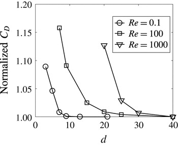
The influence of the grid resolution is tested with the flow around an isolated sphere. The normalized
 $C_{D}$
is plotted in figure 2. Three different regimes are tested: (i) Stokes flow, (ii) intermediate Reynolds number,
 $\mathit{Re}=100$
, with a steady wake and (iii) high Reynolds number,
 $\mathit{Re}=1000$
, exhibiting a complex unsteady wake, and therefore the mean drag coefficient is shown. The influence of the resolution is stronger with increasing
 $\mathit{Re}$
, as seen in figure 2. For
 $\mathit{Re}=1000$
, the observed
 $C_{D}$
at resolution
 $d_{eq}=40$
is 0.456 and is in good agreement with literature results:
 $C_{D}=0.464$
from Vakarelski et al. (Reference Vakarelski, Berry, Chan and Thoroddsen2016) and
 $C_{D}=0.48$
from Ploumhans et al. (Reference Ploumhans, Winckelmans, Salmon, Leonard and Warren2002). This resolution information is considered in maintaining the minimum thickness
 $d_{min}$
of our non-spherical particles at different
 $\mathit{Re}$
. Due to the non-sphericity, the other dimension is always larger than the minimum thickness and therefore a good particle resolution is ensured.
For a sphere, the normalized
 $C_{D}$
as a function of the diameter
 $d$
in lattice cells for different
 $\mathit{Re}$
, showing convergence of the method. The normalization is made with respect to the highest resolution
 $C_{D}$
.

3 Test of linearity for pressure and velocity fields
The drag law for Stokes flow (1.1) for non-spherical particles is based on the linearity of the Stokes equations in the creeping flow limit. As figure 1 shows, we observe that the mean
 $C_{D}$
follows the same sine-squared behaviour even in regimes with a complex unsteady wake at
 $\mathit{Re}$
as high as 2000. It has to be noted that all of the investigated geometries are axisymmetric, smooth and rounded. Although nonlinear effects dominate at higher
 $\mathit{Re}$
, we first investigate whether the inherent smooth nature of the geometries results in cancellation of nonlinearity effects in the region close to the particle surface. In other words, we test whether the velocity and pressure fields for an arbitrary particle at incident angle
 $\unicode[STIX]{x1D719}$
obey the following conditions sufficiently close to the surface:
 $$\begin{eqnarray}\displaystyle & \boldsymbol{u}_{\unicode[STIX]{x1D719}}=\boldsymbol{u}_{\unicode[STIX]{x1D719}=0^{\circ }}\cos \unicode[STIX]{x1D719}+\boldsymbol{u}_{\unicode[STIX]{x1D719}=90^{\circ }}\sin \unicode[STIX]{x1D719}, & \displaystyle\end{eqnarray}$$
 $$\begin{eqnarray}\displaystyle & p_{\unicode[STIX]{x1D719}}-p_{\infty }=(p_{\unicode[STIX]{x1D719}=0^{\circ }}-p_{\infty })\cos \unicode[STIX]{x1D719}+(p_{\unicode[STIX]{x1D719}=90^{\circ }}-p_{\infty })\sin \unicode[STIX]{x1D719}. & \displaystyle\end{eqnarray}$$
Here,
 $\boldsymbol{u}_{\unicode[STIX]{x1D719}}$
is the velocity field and
 $p_{\unicode[STIX]{x1D719}}$
is the pressure field around the particle, based on the incoming flow
 $\boldsymbol{u}_{\infty }$
oriented at angle
 $\unicode[STIX]{x1D719}$
, as shown in figure 3. If (3.1) and (3.2) are true, the corresponding drag components, i.e. the viscous drag
 $C_{D\unicode[STIX]{x1D708},\unicode[STIX]{x1D719}}$
and the pressure drag
 $C_{Dp,\unicode[STIX]{x1D719}}$
, also follow the sine-squared law.
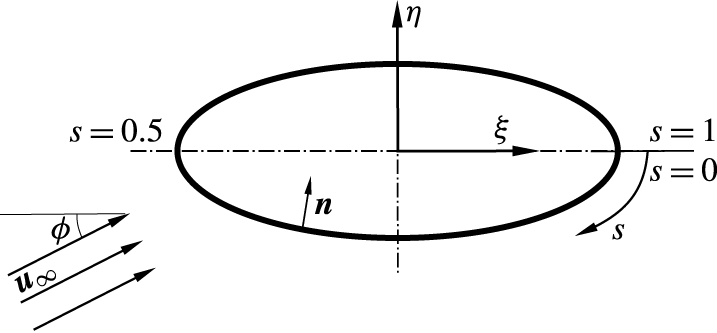
The local coordinate system (
 $\unicode[STIX]{x1D709},\unicode[STIX]{x1D702}$
) of the ellipsoidal section. Here,
 $s$
is the normalized distance along the circumference and
 $\boldsymbol{n}$
is the inward facing local unit normal vector. The simulations are performed in a rectangular domain with the particle rotated for different incident angles. For clarity and consistency, the results are analysed in the local coordinate system of the section (
 $\unicode[STIX]{x1D709},\unicode[STIX]{x1D702}$
).

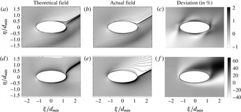
The theoretical (
 $\boldsymbol{u}_{th}$
) and actual (
 $\boldsymbol{u}_{act}$
) velocity fields and the deviation between these fields for
 $\mathit{Re}=0.1$
(a–c) and
 $\mathit{Re}=100$
(d–f). The deviation is computed as
 $\Vert \boldsymbol{u}_{th}-\boldsymbol{u}_{act}\Vert /\Vert \boldsymbol{u}_{\infty }\Vert$
in %. It should be noted that the deviation scales are different for different
 $\mathit{Re}$
.

Throughout this paper, from the three-dimensional simulations, the flow fields are analysed along the meridional plane. The meridional plane contains the axis of symmetry of the particle at different incident angles and the inflow velocity vector
 $\boldsymbol{u}_{\infty }$
. Of the different particles tested, we consider the prolate spheroid of aspect ratio
 $5/2$
for the linearity study. A special case of
 $\unicode[STIX]{x1D719}=30^{\circ }$
is tested along the meridional plane. The velocity and pressure fields from the theoretical linear combination in (3.1) and (3.2) are compared with the actual flow field from the simulations. Two cases, one for the Stokes flow at
 $\mathit{Re}=0.1$
and another exhibiting steady flow, yet sufficiently large
 $\mathit{Re}$
compared with the Stokes regime,
 $\mathit{Re}=100$
, are considered. The velocity fields based on the theory and the actual flow are given in figure 4. For Stokes flow, the linear superposition of velocity fields results in attached flow around the particle. There is a good match between the theoretical and actual fields, with deviations of up to 2 %. At
 $\mathit{Re}=100$
, the flow field exhibits attached flow for
 $\unicode[STIX]{x1D719}=0^{\circ }$
due to streamlining and a strong recirculation for
 $\unicode[STIX]{x1D719}=90^{\circ }$
. In figure 4(d), their linear combination for
 $\unicode[STIX]{x1D719}=30^{\circ }$
still appears to be attached, whereas the actual flow field as shown in figure 4(e) exhibits recirculation in the wake of the particle. There is a strong mismatch between the fields, as shown in figure 4(f), with deviations of up to 60 %.
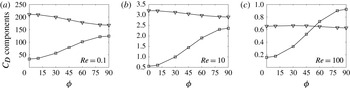
At the same time, it is interesting to note that the viscous drag force resulting from the velocity field becomes increasingly independent of the incident angle
 $\unicode[STIX]{x1D719}$
at higher
 $\mathit{Re}$
. Figure 5 shows the viscous and pressure drag components at
 $\mathit{Re}=0.1$
, 10 and 100 for the prolate spheroid of aspect ratio
 $5/2$
. Indeed, it is observed that the viscous effects become weakly dependent on the incident angle
 $\unicode[STIX]{x1D719}$
at
 $\mathit{Re}=10$
. Eventually, at
 $\mathit{Re}=100$
, the viscous drag becomes independent of
 $\unicode[STIX]{x1D719}$
compared with change in the pressure drag, with
 $C_{D\unicode[STIX]{x1D708},\unicode[STIX]{x1D719}}\approx C_{D\unicode[STIX]{x1D708},\unicode[STIX]{x1D719}=0^{\circ }}\approx C_{D\unicode[STIX]{x1D708},\unicode[STIX]{x1D719}=90^{\circ }}$
. This implies that the dependence of the drag on the incident angle of the particle,
 $\unicode[STIX]{x1D719}$
, at higher
 $\mathit{Re}$
, is purely coupled to the
 $\unicode[STIX]{x1D719}$
dependence of the pressure drag. Therefore, we next focus on the pressure coefficient on the surface of the meridional plane section.
Viscous (▿) and pressure (▫) components of the drag coefficient as a function of the incident angle
 $\unicode[STIX]{x1D719}$
at (a)
 $\mathit{Re}=0.1$
, (b)
 $\mathit{Re}=10$
and (c)
 $\mathit{Re}=100$
.

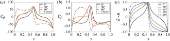
Distribution of
 $C_{p}$
against normalized distance
 $s$
along the circumference of the meridional section for (a)
 $\mathit{Re}=0.1$
and (b)
 $\mathit{Re}=100$
. (c) Surface normal projections
 $\hat{\boldsymbol{u}}\boldsymbol{\cdot }\boldsymbol{n}$
for different incident angles
 $\unicode[STIX]{x1D719}$
. It should be noted that the linearity theory matches perfectly with simulations for
 $\mathit{Re}=0.1$
and shows strong mismatch for
 $\mathit{Re}=100$
. For the different values of
 $\unicode[STIX]{x1D719}$
shown, one can note the matching trends of
 $C_{p}$
at
 $\mathit{Re}=0.1$
with
 $\hat{\boldsymbol{u}}\boldsymbol{\cdot }\boldsymbol{n}$
.

The pressure coefficient is defined as
 $C_{p}=(p-p_{\infty })/(1/2\unicode[STIX]{x1D70C}|\boldsymbol{u}_{\infty }|^{2})$
, with pressure
 $p$
measured on the surface and
 $p_{\infty }$
the pressure at the far field. The pressure coefficient
 $C_{p}$
is plotted as a function of the distance
 $s$
along the circumference of the meridional section, normalized with the section circumference, as shown in figure 3. The
 $C_{p}$
distributions on the section along the meridional plane of the spheroid are plotted for
 $\mathit{Re}=0.1$
and
 $\mathit{Re}=100$
in figures 6(a) and 6(b) respectively. Referring to figure 3, the
 $\boldsymbol{u}_{\infty }$
at
 $\unicode[STIX]{x1D719}=0^{\circ }$
is along the
 $+\unicode[STIX]{x1D709}$
axis, and the
 $C_{p}$
peaks are observed near
 $s=0.5$
in figure 6(a,b), which is at the leading edge of the spheroid for that incident angle. At
 $\mathit{Re}=0.1$
, we observe an exact match between
 $C_{p}$
using the linearity theory (3.2) and the actual simulation for
 $\unicode[STIX]{x1D719}=30^{\circ }$
. At
 $\mathit{Re}=100$
, the actual
 $C_{p}$
distribution for
 $\unicode[STIX]{x1D719}=30^{\circ }$
is different compared with the distribution based on linearity theory, as seen in figure 6(b). Therefore, it can be concluded that it is not due to linearity that the drag law shows sine-squared behaviour at higher
 $\mathit{Re}$
.
4 Reason for the sine-squared drag law at higher
 $\mathit{Re}$

Again, we consider the meridional section of the prolate spheroid of aspect ratio
 $5/2$
for this study. We hypothesize that the
 $C_{p}$
distribution takes the form
 $$\begin{eqnarray}\displaystyle & C_{p}=-m+(1+m)(\hat{\boldsymbol{u}}\boldsymbol{\cdot }\boldsymbol{n})^{k}. & \displaystyle\end{eqnarray}$$
Here,
 $m$
and
 $k$
are constants,
 $\hat{\boldsymbol{u}}=\boldsymbol{u}_{\infty }/|\boldsymbol{u}_{\infty }|$
is the orientation of the far-field flow direction and
 $\boldsymbol{n}$
is the inward facing local unit normal vector, as in figure 3. The above form
 $-m+(1+m)(\hat{\boldsymbol{u}}\boldsymbol{\cdot }\boldsymbol{n})^{k}$
is inspired by the inviscid flow around a sphere, where
 $C_{p}=1-c\sin ^{2}\unicode[STIX]{x1D703}$
, with
 $c=9/4$
and the
 $\unicode[STIX]{x1D703}$
measured from the stagnation point. For a sphere,
 $\hat{\boldsymbol{u}}\boldsymbol{\cdot }\boldsymbol{n}=\cos \unicode[STIX]{x1D703}$
, and rearranging terms with
 $m=c-1$
, the
 $C_{p}$
distribution for a sphere becomes
 $C_{p}=-m+(1+m)(\hat{\boldsymbol{u}}\boldsymbol{\cdot }\boldsymbol{n})^{2}$
. A more general form is considered in our case with an arbitrary exponent
 $k$
.
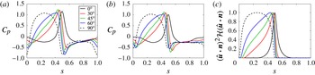
Distributions of
 $C_{p}$
at (a)
 $\mathit{Re}=100$
and (b)
 $\mathit{Re}=2000$
(time averaged), and (c) second-power surface normal projections
 $(\hat{\boldsymbol{u}}\boldsymbol{\cdot }\boldsymbol{n})^{2}{\mathcal{H}}(\hat{\boldsymbol{u}}\boldsymbol{\cdot }\boldsymbol{n})$
versus the normalized distance
 $s$
along the circumference of the meridional section for different values of
 $\unicode[STIX]{x1D719}$
.

The term
 $-m$
acts as a negative offset and the term
 $(1+m)$
acts as a scaling factor, such that
 $C_{p}=1$
at the stagnation point (
 $\hat{\boldsymbol{u}}\boldsymbol{\cdot }\boldsymbol{n}=1$
), as would be expected from Bernoulli’s law at the point where
 $\boldsymbol{u}=\mathbf{0}$
. For increasing
 $\mathit{Re}$
, the high-pressure region localizes more around the stagnation point, and this can be confirmed by comparing the
 $C_{p}$
distribution for
 $\unicode[STIX]{x1D719}=0^{\circ }$
at
 $\mathit{Re}=0.1$
and 100 in figures 6(a) and 6(b) respectively. Moreover, for
 $\mathit{Re}\gg 1$
, figure 7(a,b) shows that the dominant part of the pressure drag originates from the front side of the particle (
 $\hat{\boldsymbol{u}}\boldsymbol{\cdot }\boldsymbol{n}>0$
, see figure 6
c), and therefore we focus on this region. For
 $\mathit{Re}\gg 1$
, we choose
 $k=2$
. The value
 $k=2$
is inspired by inviscid irrotational flow theory, as discussed above, although the flow is not exactly inviscid. The distributions of
 $C_{p}$
for
 $Re=100$
,
 $Re=2000$
(time averaged) and
 $(\hat{\boldsymbol{u}}\boldsymbol{\cdot }\boldsymbol{n})^{2}{\mathcal{H}}(\hat{\boldsymbol{u}}\boldsymbol{\cdot }\boldsymbol{n})$
are given in figures 7(a), 7(b) and 7(c) respectively. Here,
 ${\mathcal{H}}$
is the Heaviside step function, given by
 $$\begin{eqnarray}\displaystyle {\mathcal{H}}(x)=\left\{\begin{array}{@{}ll@{}}1\quad & \text{if}~x>0,\\ 0\quad & \text{otherwise}.\end{array}\right. & & \displaystyle\end{eqnarray}$$
The term
 ${\mathcal{H}}(\hat{\boldsymbol{u}}\boldsymbol{\cdot }\boldsymbol{n})$
is introduced above to consider only the front side of the particle projected to the inflow.
It can be observed that the maximum values of
 $C_{p}$
for different values of
 $\unicode[STIX]{x1D719}$
are nearly the same and close to 1, as expected at the stagnation point in inviscid flow. Moreover, the overall trends of the
 $C_{p}$
curves in figure 7(a,b) and the
 $(\hat{\boldsymbol{u}}\boldsymbol{\cdot }\boldsymbol{n})^{2}{\mathcal{H}}(\hat{\boldsymbol{u}}\boldsymbol{\cdot }\boldsymbol{n})$
in figure 7(c) are almost similar, including the trends of curvature. Actually, for the pressure drag, we specifically need to look at the surface projection of
 $C_{p}$
along the flow direction, i.e.
 $C_{p,drag}=C_{p}\hat{\boldsymbol{u}}\boldsymbol{\cdot }\boldsymbol{n}$
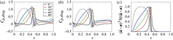
. The similarity between
 $C_{p,drag}$
and
 $(\hat{\boldsymbol{u}}\boldsymbol{\cdot }\boldsymbol{n})^{3}$
for different angles can be observed in figure 8(a–c). The trends agree well for different incident angles. Further, the
 $C_{p}$
and
 $C_{p,drag}$
distributions for
 $\mathit{Re}=100$
and
 $\mathit{Re}=2000$
indicate that they are self-similar and independent of
 $\mathit{Re}$
, at least for the front side of the particle (
 $\hat{\boldsymbol{u}}\boldsymbol{\cdot }\boldsymbol{n}>0$
). It should be noted that the influence of the offset
 $m$
is less significant for
 $C_{p,drag}$
than it is for
 $C_{p}$
. Moreover, the precise value of
 $m$
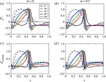
may be position- and incident-angle-dependent, but its variation is negligible compared with the overall variation in the pressure drag. This is shown explicitly in figure 9, where the measured
 $C_{p}$
distributions are compared with our proposed
 $C_{p}$
form computed as
 $C_{p}=-m+(1+m)(\hat{\boldsymbol{u}}\boldsymbol{\cdot }\boldsymbol{n})^{2}{\mathcal{H}}(\hat{\boldsymbol{u}}\boldsymbol{\cdot }\boldsymbol{n})$
and the
 $C_{p,drag}$
accordingly. It can be observed that the value of
 $m$
influences
 $C_{p}$
considerably. However, its influence on
 $C_{p,drag}$
is much weaker, and, therefore, we proceed with
 $m=0$
in upcoming steps.
Distributions of
 $C_{p,drag}$
at (a)
 $\mathit{Re}=100$
and (b)
 $\mathit{Re}=2000$
(time averaged), and (c) third-power surface normal projections
 $(\hat{\boldsymbol{u}}\boldsymbol{\cdot }\boldsymbol{n})^{3}{\mathcal{H}}(\hat{\boldsymbol{u}}\boldsymbol{\cdot }\boldsymbol{n})$
versus the normalized distance
 $s$
along the circumference of the meridional section for different values of
 $\unicode[STIX]{x1D719}$
.

Quantitative comparison of the
 $C_{p}$
(a,b) and
 $C_{p,drag}=C_{p}\hat{\boldsymbol{u}}\boldsymbol{\cdot }\boldsymbol{n}$
(c,d) from the proposed theory ((4.1), thin lines) with the actual measurements at
 $\mathit{Re}=2000$
(thick lines). We used
 $m=0$
(a,c) and
 $m=0.3$
(b,d). It should be noted that the influence of the value of
 $m$
is weaker for
 $C_{p,drag}$
compared with
 $C_{p}$
.

The term
 $C_{p,drag}$
corresponds to the local contribution of pressure to the sectional pressure drag. Therefore, we require integrals to compute the total pressure drag due to this section. We define the integral of
 $k\text{th}$
power of projection
 $\hat{\boldsymbol{u}}\boldsymbol{\cdot }\boldsymbol{n}$
for the front side of the section as
 $$\begin{eqnarray}\displaystyle b_{k}=\int _{0}^{1}(\hat{\boldsymbol{u}}\boldsymbol{\cdot }\boldsymbol{n})^{k}{\mathcal{H}}(\hat{\boldsymbol{u}}\boldsymbol{\cdot }\boldsymbol{n})\,\text{d}s. & & \displaystyle\end{eqnarray}$$
An interesting property is that the integral of the second power of projection,
 $b_{2}$
, exactly obeys sine-squared behaviour for different values of
 $\unicode[STIX]{x1D719}$
. This can be written as
 $b_{2,\unicode[STIX]{x1D719}}=b_{2,\unicode[STIX]{x1D719}=0^{\circ }}+(b_{2,\unicode[STIX]{x1D719}=90^{\circ }}-b_{2,\unicode[STIX]{x1D719}=0^{\circ }})\sin ^{2}\unicode[STIX]{x1D719}$
and is shown in figure 10(a). This law holds for the family of ellipsoidal sections and is independent of aspect ratio. This can also be confirmed from the fact that the
 $C_{p}$
distribution is proportional to
 $\hat{\boldsymbol{u}}\boldsymbol{\cdot }\boldsymbol{n}$
in Stokes flow (see figure 6
a,c) and therefore
 $C_{p,drag}=C_{p}\hat{\boldsymbol{u}}\boldsymbol{\cdot }\boldsymbol{n}$
is proportional to
 $(\hat{\boldsymbol{u}}\boldsymbol{\cdot }\boldsymbol{n})^{2}$
.
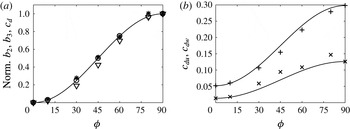
For a prolate spheroid of aspect ratio
 $5/2$
: (a) the normalized
 $b_{2,\unicode[STIX]{x1D719}}$
(○),
 $b_{3,\unicode[STIX]{x1D719}}$
(▿), sectional pressure drag
 $c_{d,\unicode[STIX]{x1D719}}$
at
 $\mathit{Re}=2000$
(*) and
 $\sin ^{2}\unicode[STIX]{x1D719}$
(solid line); (b) components of sectional pressure drag
 $c_{d,\unicode[STIX]{x1D719}}$
at
 $\mathit{Re}=2000$
decomposed into upstream drag
 $c_{du,\unicode[STIX]{x1D719}}$
(
 $+$
) and wake side drag
 $c_{dw,\unicode[STIX]{x1D719}}$
(
 $\times$
), together with their corresponding sine-squared interpolating curves. It should be noted that the trends of
 $b_{3,\unicode[STIX]{x1D719}}$
and
 $c_{du,\unicode[STIX]{x1D719}}$
are similar, both under their respective sine-squared curves.

As per our earlier observation, at higher
 $\mathit{Re}$
, the
 $C_{p,drag}$
distribution is proportional to
 $(\hat{\boldsymbol{u}}\boldsymbol{\cdot }\boldsymbol{n})^{3}$
. However, the integral
 $b_{3,\unicode[STIX]{x1D719}}$
does not exactly hold sine-squared behaviour, as shown in figure 10(a). It trends slightly below the sine-squared curve. The equivalent of
 $b_{3,\unicode[STIX]{x1D719}}$
is the sectional pressure drag from the upstream side of the section, which we compare in the upcoming steps. We define sectional pressure drag integrated over the circumference of an ellipsoidal section as
 $$\begin{eqnarray}\displaystyle c_{d}=\int _{0}^{1}C_{p,drag}\,\text{d}s. & & \displaystyle\end{eqnarray}$$
We then decompose
 $c_{d}$
into upstream side (
 $c_{du}$
) and wake side (
 $c_{dw}$
) as
 $$\begin{eqnarray}\displaystyle & \displaystyle c_{du}=\int _{0}^{1}C_{p,drag}{\mathcal{H}}(\hat{\boldsymbol{u}}\boldsymbol{\cdot }\boldsymbol{n})\,\text{d}s\quad \text{and}\quad c_{dw}=\int _{0}^{1}C_{p,drag}{\mathcal{H}}(-\hat{\boldsymbol{u}}\boldsymbol{\cdot }\boldsymbol{n})\,\text{d}s. & \displaystyle\end{eqnarray}$$
The above integrals for different incident angles
 $\unicode[STIX]{x1D719}$
, i.e.
 $c_{du,\unicode[STIX]{x1D719}}$
and
 $c_{dw,\unicode[STIX]{x1D719}}$
, for
 $\mathit{Re}=2000$
are plotted in figure 10(b) together with their corresponding sine-squared interpolation curves based on the end values. As seen from figure 10(a,b), the upstream drag
 $c_{du,\unicode[STIX]{x1D719}}$
trend is very similar to
 $b_{3,\unicode[STIX]{x1D719}}$
and both are slightly below their respective sine-squared curves. At the same time, the wake-induced drag component
 $c_{dw,\unicode[STIX]{x1D719}}$
values are slightly above their respective sine-squared curves at the intermediate angles, i.e.
 $0^{\circ }<\unicode[STIX]{x1D719}<90^{\circ }$
. Therefore, the wake drag adequately compensates the upstream drag proportionately at the intermediate angles, thereby making the total section drag appear to scale in a sine-squared manner. The normalized sectional pressure drag
 $c_{d,\unicode[STIX]{x1D719}}$
for different angles for
 $\mathit{Re}=2000$
itself follows a near sine-squared pattern, as shown in figure 10(a). The spheroid by itself is made of different such ellipsoidal sections, each obeying sine-squared behaviour of different scales and altogether giving the total drag sine-squared behaviour. We have tested the reasoning in this section for different aspect ratio prolate spheroids, and found similar dependences of
 $C_{p,drag}$
with
 $(\hat{\boldsymbol{u}}\boldsymbol{\cdot }\boldsymbol{n})^{3}{\mathcal{H}}(\hat{\boldsymbol{u}}\boldsymbol{\cdot }\boldsymbol{n})$
for different values of
 $\unicode[STIX]{x1D719}$
.
4.1 Limitations and comments
In the introduction, we showed results for prolate spheroids of different aspect ratios and an oblate spheroid of aspect ratio
 $5/2$
. However, increasing the aspect ratio for an oblate spheroid results in an increasing digression from the sine-squared drag law, even at moderate
 $\mathit{Re}$
. The
 $C_{D}$
results for an oblate spheroid of aspect ratio 4 at
 $\mathit{Re}=100$
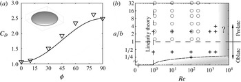
are presented in figure 11(a). Clearly, a non-monotonic dependence of
 $C_{D}$
on the incidence angle
 $\unicode[STIX]{x1D719}$
is observed. The observed maximum deviation is around 10 % at
 $\unicode[STIX]{x1D719}=60^{\circ }$
against the sine-squared curve. The reason why the drag law fails for flatter discs can be explained by our earlier observation that the wake has a higher drag contribution at intermediate angles
 $0^{\circ }<\unicode[STIX]{x1D719}<90^{\circ }$
(see
 $c_{dw}$
in figure 10
b) when compared with the sine-squared curve. The flat-disc-like geometry experiences a stronger wake, amplifying the effect strongly. If we assume a 10 % deviation to be the limit of applicability, the oblate spheroid of aspect ratio 4 is at the bounding limit for the drag law. On the other hand, prolate spheroids of larger aspect ratio, as shown in the introduction, still obey the sine-squared behaviour even at
 $\mathit{Re}=2000$
, due to the weaker wake side drag. A sketch of the plausible valid region of the sine-squared behaviour is shown in figure 11(b). We have also tested a capsule-like spherocylinder of aspect ratio 4 and it also exhibits sine-squared drag scaling at high
 $\mathit{Re}$
, due to a closer resemblance to a prolate spheroid. The
 $C_{D}$
results from this work will be published as correlations dependent on
 $\mathit{Re}$
and
 $\unicode[STIX]{x1D719}$
in a separate paper. Since the prolate spheroid of aspect ratio 4 is simulated only for
 $\mathit{Re}=2000$
, the corresponding results are given here, with
 $C_{D,\unicode[STIX]{x1D719}=0^{\circ }}=0.147$
and
 $C_{D,\unicode[STIX]{x1D719}=90^{\circ }}=1.105$
.
(a) Plot of
 $C_{D}$
against
 $\unicode[STIX]{x1D719}$
at
 $\mathit{Re}=100$
for an oblate spheroid of aspect ratio 4 (▿) and the corresponding sine-squared interpolating curve (solid line); (b) the tested data points (
 $+$
) and the plausible valid region for sine-squared scaling (unshaded). The valid region is based on our results and the data of Ouchene et al. (Reference Ouchene, Khalij, Arcen and Tanière2016) for prolate spheroids up to aspect ratios of 32 and
 $\mathit{Re}=240$
(○). The ratio
 $a/b$
is the ratio of lengths parallel and orthogonal to the axis of rotation.

The
 $\mathit{Re}=2000$
limit for the tested particles is rather limited by the LBM solver and not by the flow physics itself. We believe that the drag law might hold to even higher
 $\mathit{Re}$
. However, flow fields are indeed complex for high
 $\mathit{Re}$
and the extent to which the drag law is valid needs further investigation. For example, Jiang et al. (Reference Jiang, Gallardo, Andersson and Zhang2015) simulated flow around a 6 : 1 prolate spheroid at
 $\unicode[STIX]{x1D719}=45^{\circ }$
at
 $\mathit{Re}=3000$
based on the minor diameter. They reported a side force, almost 75 % of the magnitude of the drag force, perpendicular to the meridional plane. This indicates that the flow is highly asymmetric about the meridional plane. However, they did not investigate the incident angle dependence of the drag force. To what extent their reported flow asymmetries might influence the sine-squared drag behaviour is not yet known and therefore needs further investigation.
5 Lift forces
Besides drag, any non-spherical particle at an inclination with respect to a uniform flow will experience lift. Here, we provide a concise section with interesting observations and comments regarding the lift forces.
We define the lift coefficient as
 $C_{L}=|\boldsymbol{F}_{L}|/((1/2)\unicode[STIX]{x1D70C}|\boldsymbol{u}_{\infty }|^{2}(\unicode[STIX]{x03C0}/4)d_{eq}^{2})$
, with
 $F_{L}$
being the measured lift force. For a particle in the Stokes regime, based on linearity theory, the
 $C_{L}$
at an incident angle
 $\unicode[STIX]{x1D719}$
is
 $$\begin{eqnarray}\displaystyle C_{L,\unicode[STIX]{x1D719}}=(C_{D,\unicode[STIX]{x1D719}=90^{\circ }}-C_{D,\unicode[STIX]{x1D719}=0^{\circ }})\sin \unicode[STIX]{x1D719}\cos \unicode[STIX]{x1D719}. & & \displaystyle\end{eqnarray}$$
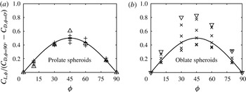
The normalized lift coefficient
 $C_{L,\unicode[STIX]{x1D719}}/(C_{D,\unicode[STIX]{x1D719}=90^{\circ }}-C_{D,\unicode[STIX]{x1D719}=0^{\circ }})$
plotted against the incident angle
 $\unicode[STIX]{x1D719}$
. The solid line indicates
 $\sin \unicode[STIX]{x1D719}\cos \unicode[STIX]{x1D719}$
. (a) Prolate spheroid of aspect ratio
 $5/2$
for
 $\mathit{Re}=0.1$
, 10, 100, 1000 and 2000 (
 $+$
); prolate spheroid of aspect ratio 4 at
 $\mathit{Re}=2000$
(▵); (b) oblate spheroid of aspect ratio
 $5/2$
for
 $\mathit{Re}=0.1$
, 10, 100, 1000 and 2000 (
 $\times$
); oblate spheroid of aspect ratio 4 at
 $\mathit{Re}=100$
(▿). It should be noted that the oblate spheroids are experiencing stronger deviations compared with prolate spheroids.

From our experience of the different non-spherical particles tested, equation (5.1) is still a reasonable approximation in the complete absence of
 $C_{L}$
data for prolate spheroids, even at high
 $\mathit{Re}$
, as seen in figure 12(a). The average of the absolute deviations between
 $C_{L,\unicode[STIX]{x1D719}}$
from the simulations and (5.1) is less than 15 % for the tested prolate spheroids at different
 $\mathit{Re}$
. For oblate spheroids, with increasing aspect ratios, the deviations increase more, as seen in figure 12(b). For the oblate spheroid of aspect ratio 4 at
 $\mathit{Re}=100$
, the simulated
 $C_{L}$
is much larger, by around 60 %, than the theory for the reasons already observed in figure 10(b). Similarly to the drag, the wake-induced force is also contributing strongly to the lift and thereby making the observed
 $C_{L}$
much larger than the theory at intermediate incident angles.
There are different reasons why the incident angle dependence of the lift coefficient
 $C_{L}$
cannot be exactly quantified in a predictable fashion like that of
 $C_{D}$
. The order of magnitude of the lift coefficient depends on the difference of
 $C_{D}$
at two extreme incident angles, i.e.
 $(C_{D,\unicode[STIX]{x1D719}=90^{\circ }}-C_{D,\unicode[STIX]{x1D719}=0^{\circ }})$
, and goes to zero at the extreme ends of incident angles, i.e. at
 $\unicode[STIX]{x1D719}=0^{\circ }$
,
 $90^{\circ }$
. However, for
 $C_{D}$
at different incident angles
 $\unicode[STIX]{x1D719}$
, apart from the
 $C_{D}$
difference term, there is an additional term giving a constant offset, i.e.
 $C_{D}$
at
 $\unicode[STIX]{x1D719}=0^{\circ }$
. This implies that the variation of
 $C_{L,\unicode[STIX]{x1D719}}$
is much more sensitive than that of
 $C_{D,\unicode[STIX]{x1D719}}$
. Therefore, any variation in pressure distribution at higher
 $\mathit{Re}$
would be more amplified for
 $C_{L}$
than for
 $C_{D}$
. The
 $C_{L}$
results from this work will be published as correlations dependent on
 $\mathit{Re}$
and
 $\unicode[STIX]{x1D719}$
in a separate paper.
6 Conclusion
The flow around prolate and oblate spheroids of different aspect ratios was studied. We explored the sine-squared drag law in detail with a prolate spheroid of aspect ratio
 $5/2$
. We found that the reason for the drag law at high
 $\mathit{Re}$
is not due to linearity theory, which results in an identical drag law in the Stokes regime. At high
 $\mathit{Re}$
, the viscous drag becomes almost independent of the incident angle
 $\unicode[STIX]{x1D719}$
and the pressure drag is the only factor influenced by the incident angle
 $\unicode[STIX]{x1D719}$
. At high
 $\mathit{Re}$
, the pressure distribution contributing to the drag shows a dependence on the surface normal orientation with the incoming flow in a consistent pattern, as discussed. Prolate spheroids of higher aspect ratios follow the sine-squared pattern even at
 $\mathit{Re}=2000$
. Oblate spheroids of aspect ratio 4 or larger do not exhibit the sine-squared pattern due to strong wake-induced drag. Regarding lift coefficients, we find that the theoretical
 $C_{L}$
equation can provide a reasonable approximation, even at high
 $\mathit{Re}$
, for prolate spheroids.
Both the drag law, valid at high
 $\mathit{Re}$
for the prolate spheroids and low-aspect-ratio oblate spheroids, and the lift law for the prolate spheroids hold good potential for different applications. For example, they are very useful for Euler–Lagrangian flow simulations of non-spherical particles. Any particle-shape-specific
 $C_{D}$
and
 $C_{L}$
for a given
 $\mathit{Re}$
at different
 $\unicode[STIX]{x1D719}$
, even at high
 $\mathit{Re}$
, can be obtained by performing just two simulations:
 $C_{D}$
at
 $\unicode[STIX]{x1D719}=0^{\circ }$
and
 $\unicode[STIX]{x1D719}=90^{\circ }$
.
Acknowledgements
The authors thank the European Research Council for its financial support under its consolidator grant scheme, contract no. 615906 (NonSphereFlow). The simulations were performed in LB3D code with additional improvements. We thank Professor J. Harting for providing the code and Professor J. A. M. Kuipers for fruitful discussions. The first author thanks Dr A. Zarghami and Q. Xie for the interesting discussions on LBM. The work has been made possible by a grant for computation time, project number SH-351-15, financed by the Netherlands Organisation for Scientific Research (NWO).