





1. Introduction
Adding a small amount of polymers into Newtonian turbulent channel/pipe flows can reduce their flow drag significantly. A lot of research has been carried out on turbulent drag reduction (TDR) since Toms (Reference Toms1949) found this effect, but the mechanism about TDR still remains under debate. Among these studies, Virk et al. (Reference Virk, Merril, Mickley and Smith1967) and Virk (Reference Virk1971) reported two important findings about TDR: the onset of drag reduction (DR) and the existence of the maximum drag reduction (MDR) limit. The former means that TDR does not occur unless the fluid elasticity exceeds a certain degree. Once TDR occurs, the flow drag decreases gradually with a further increase of fluid elasticity. In most cases, the Newtonian inertial turbulence (IT) usually cannot be completely eliminated at moderate and high Reynolds numbers (Re), and the flow drag eventually saturates to a level between the magnitudes of Newtonian IT and laminar flow, which is known as the MDR limit. Contrary to intuition, Virk (Reference Virk1971) reported that the MDR limit depends solely on the Reynolds number (Re) regardless of which type of polymer additive is used, which has been widely recognized. However, recent studies (see Choueiri, Lopez & Hof Reference Choueiri, Lopez and Hof2018; Pereira, Thompson & Mompean Reference Pereira, Thompson and Mompean2019) found that polymers could completely eliminate the IT, and give way to laminar flow with the MDR limit being exceeded when IT is weak at low Re. It challenges the existence and universality of the MDR limit and further deepens the mystery of the MDR phenomenon. According to the identification of MDR flow essence, the interpretation of MDR can be generally divided into two categories.
The first believes that the drag-reducing turbulence (DRT) from onset to the MDR state is always a Newtonian IT modulated by polymers. In fact, this essential understanding has dominated the research on TDR for decades since the TDR effect was discovered. From this starting point, many theories and hypotheses for DR have been proposed, such as the classical viscous theory by Lumley (Reference Lumley1969,Reference Lumley1973) and the elastic theory by Tabor & de Gennes (Reference Tabor and de Gennes1986) and De Gennes & Badoz (Reference De Gennes and Badoz1996). Although these phenomenological theories have not been fully supported, they all believe that the DR effect comes from the modulation on turbulent structures by polymers. Furthermore, the classical ‘effective slip’ hypothesis proposed by Virk (Reference Virk1975) gave a straightforward interpretation for the MDR phenomenon. Under this hypothesis, it was believed that the buffer layer (or the so-called ‘elastic sublayer’) in between the laminar (viscous) sublayer and turbulent bulk region can be enlarged by polymers to form an effective slip on the velocity profile in the turbulent bulk region, which indicates the occurrence of the DR phenomenon. When the buffer layer is extended to the pipe/channel centre, the flow pattern converges, which means the occurrence of the MDR phenomenon.
Against this backdrop, Xi & Graham (Reference Xi and Graham2011) further explained the potential turbulent dynamics in the MDR state with the so-called minimal flow unit (MFU) method (see Xi & Graham Reference Xi and Graham2010). Benefiting from this MFU method, they discovered that the dynamics in DRT flow undergoes transitions between ‘hibernating’ events with low flow drag and ‘active’ events with high flow drag. The active state means that flow has the basic characteristics of Newtonian IT such as coherent structures (e.g. velocity streaks, quasi-streamwise vortices, hairpin vortices) and high flow drag, while the hibernating state shows many features in the MDR state: weak three dimensionality with weak streamwise vortices and low-speed streaks as well as a converged mean velocity profile. It was found that hibernating periods become more frequent with an increase of Wi because polymers are more likely to be stretched to modulate dynamics in IT until the flow enters the MDR state. Thus, Xi & Graham (Reference Xi and Graham2011) argued that the MDR is a flow state where the hibernating turbulence becomes the norm. As for the active turbulence in the MDR state, it cannot be completely eliminated since vortices in hibernating turbulence are too weak to maintain the high extension state of polymers continuously. Furthermore, the hibernating events are hardly modulated by polymers due to weak extension, which well explains the reason why the MDR limit is not affected by changing polymer properties.
The second considers the MDR state, the ultimate state of DRT, to be a regime of elasto-inertial turbulence (EIT). In the early days, Warholic, Massah & Hanratty (Reference Warholic, Massah and Hanratty1999) noticed a very unusual phenomenon in DRT experiments: the turbulence can survive well in the MDR state although the Reynolds shear stress nearly disappears, which is in great contradiction with IT-related dynamics. Sreenivasan & White (Reference Sreenivasan and White2000) also found that the elastic energy stored in polymers becomes comparable to turbulent kinetic energy (TKE) at the MDR state through scaling analysis. Furthermore, Min et al. (Reference Min, Yoo, Choi and Joseph2003) pointed out that the energy for turbulent maintenance at this ultimate state of DRT comes from energy transferred from polymers to turbulent fluctuations. Based on these early studies, it is suspected that polymers play an important role in sustaining turbulence in the MDR state. Thus, it is worth conjecturing whether polymers can induce chaotic flows actively or not.
Groisman & Steinberg (Reference Groisman and Steinberg2000) focused on the role of the elastic nonlinearity of polymers and proposed a new chaotic flow state, called elastic turbulence (ET). Inspired by ET, Dubief and his coworkers proposed a new turbulence state, which is called EIT, in inertial pipe/channel flows with polymers at moderate Re (see Dubief, Terrapon & Julio Reference Dubief, Terrapon and Julio2013; Samanta et al. Reference Samanta, Dubief, Holzner, Schafer, Morozov, Wagner and Hof2013). Unlike IT, EIT is triggered by the interaction between elastic instability and the flow inertia. The most identified feature is the emergence of trains of small-scale spanwise vortex structures with alternating sign that appear on elongated sheets of highly stretched polymers in the streamwise direction with a small upward tilt. Dubief et al. (Reference Dubief, Terrapon and Julio2013) suggested that these sheets are caused by the unstable nature of nonlinear polymer advection, which could lead to local low-speed jet-like flows due to the significant increase of extensional viscosity in these regions. Spanwise vortex structures are formed by pressure from local jet-like flows that produce sheets affected by unstable advection. The above links constitute a self-sustaining cycle for EIT. Through decomposing pressure fluctuations into rapid, slow and polymer parts, Terrapon, Dubief & Soria (Reference Terrapon, Dubief and Soria2015) confirmed that those small-scale spanwise vortex structures associated with sheets are driven by polymers directly. Recently, we focused on the anisotropy in EIT and pictured the self-sustaining energy process (see Zhang et al. Reference Zhang, Zhang, Wang, Li, Yu and Li2022). It was found that sheet-like structures in the streamwise direction are caused by the interaction between polymers and turbulent fluctuations, and work done by elastic stress provides energy for their maintenance. Regarding the origin of EIT, there is still a dispute between the ‘wall mode’ (see Garg et al. Reference Garg, Chaudhary, Khalid, Shankar and Subramanian2018; Shekar et al. Reference Shekar, McMullen, Wang, Mckeon and Graham2019, Reference Shekar, McMullen, McKeon and Graham2020, Reference Shekar, McMullen, McKeon and Graham2021; Choueiri et al. Reference Choueiri, Lopez, Varshney, Sankar and Hof2021) and the ‘centre mode’ (see Chaudhary et al. Reference Chaudhary, Garg, Shankar and Subramanian2019; Page, Dubief & Kerswell Reference Page, Dubief and Kerswell2020). In this regard, although not explicitly stated, it seems that the original simulation of EIT done by Dubief and his coworkers (Dubief et al. Reference Dubief, Terrapon and Julio2013; Terrapon et al. Reference Terrapon, Dubief and Soria2015) originates from a ‘wall mode’ according to the characteristics of the flow fields and the polymer extension structures therein. Although the results of Page et al. (Reference Page, Dubief and Kerswell2020) covered both ‘wall mode’ and ‘centre mode’, they show a link between the EIT and the ‘centre mode’ in their investigated parameter space.
As for the link between the MDR state and EIT regime, some studies provide evidence that the characteristic structures of EIT could be observed in MDR flows. The pioneering experiments and numerical simulations by Samanta et al. (Reference Samanta, Dubief, Holzner, Schafer, Morozov, Wagner and Hof2013) and Dubief et al. (Reference Dubief, Terrapon and Julio2013) found that when the flow enters the MDR state with an increase of Wi, DRT flows show similar flow characteristics as observed in EIT – trains of spanwise vortices accompanied by sheets of polymer extension. Recently we found that the DRT flows of Oldroyd-B fluid show the characteristics of centre-mode-dominated structures in EIT – quasi-arrow-like extension structures through direct numerical simulation (DNS) at high Wi (see Zhang et al. Reference Zhang, Zhang, Li, Yu and Li2021a,Reference Zhang, Shao, Li, Ma, Zhang and Lib, Reference Zhang, Zhang, Wang, Li, Yu and Li2022). By adjusting the concentration of the polymer solution in pipe flow experiments at low Re, Choueiri et al. (Reference Choueiri, Lopez and Hof2018) found that IT-related dynamics could be eliminated and the flow turns to be a laminar regime breaking through the MDR limit with an increase of polymer concentration. With further increasing solution concentration, the flow enters the turbulent state again, and the flow drag converges gradually to the MDR state. The above phenomenon directly proves that the MDR flow is essentially a regime of EIT. Furthermore, we introduced the Renard–Deck (RD) identity (see Renard & Deck Reference Renard and Deck2016) (used for the contribution decomposition of flow drag) into turbulent channel flow and developed a characterization method for IT-related dynamics and EIT-related dynamics in DRT (Zhang et al. Reference Zhang, Zhang, Li, Yu and Li2021d). The research results based on this framework and the Oldroyd-B model show that the EIT-related dynamics begin to play a role long before the flow enters the MDR state. Thus, DRT is identified as a result of the interaction between IT-related dynamics and EIT-related dynamics. Based on this, we re-pictured DRT and constructed a self-sustaining cycle for DRT where dynamics of IT and EIT coexist in the flow. It turned out that IT-related dynamics almost disappear at the MDR state (Zhang et al. Reference Zhang, Zhang, Wang, Li, Yu and Li2022).
The MDR phenomenon has long been a mystery and challenges the understanding of the DRT mechanism as well as its modelling. The above two viewpoints give completely different explanations for the MDR phenomenon, and both of them seem reasonable since the hibernation state and EIT regime all can provide a barrier to prevent laminarization for DRT. In addition, recent studies (Zhu & Xi Reference Zhu and Xi2021; Zhang et al. Reference Zhang, Zhang, Wang, Li, Yu and Li2022) found that the dynamics continue to develop with an increase of Wi even if the flow enters the MDR state. Considering that the MDR limit can be exceeded at low Re (Choueiri et al. Reference Choueiri, Lopez and Hof2018; Pereira et al. Reference Pereira, Thompson and Mompean2019), it is very necessary to reexamine the universality of the MDR phenomenon – the same MDR limit for different polymer solution properties. To further promote the understanding of the essence of the MDR state, this paper focuses on nonlinear extension effects on the dynamics of MDR and conducts a series of DNS of viscoelastic DRT at a modest Reynolds number Re with  $Re = 6000$ for the FENE-P model that covers a wide range of flow states. The following parts are organized as follows: § 2 introduces the governing equations of viscoelastic fluid flow, numerical methods and conditions; § 3 presents the numerical results and analyses the nonlinear extension effects on statistical properties, energy spectrum, structures and the energy budgets; § 4 discusses the mechanisms of the nonlinear extension effect obtained; § 5 gives the conclusions.
2. Methods
2.1. Computational domain and governing equations
This study focuses on the viscoelastic channel flow between two parallel plates as shown in figure 1. The channel height in the Cartesian coordinate system is  $2h$ and with the corresponding velocity components of
 $u$,
 $v$ and
 $w$ in the streamwise
 $x$, wall-normal
 $y$ and spanwise
 $z$ directions, respectively. Assuming that the fluid is incompressible, the characteristic length, velocity, time, pressure and additional stress are set to be
 $h$,
 $u_b = ({1}/{2h})\int _0^{2h} U\,{\rm d}y$ (
 $U$ is the local mean velocity in the streamwise direction),
 $h/u_b$ and
 $\rho u_b^2$, respectively. Neglecting the volume force, the dimensionless governing equations for viscoelastic fluid flow with the FENE-P model based on the outer scale are obtained,
 $$\begin{gather} \frac{{\partial u_i }}{{\partial x_i }} = 0, \end{gather}$$
 $$\begin{gather}\frac{{\partial u_i }}{{\partial t }} + {u_j} \frac{{\partial u_i}}{{\partial x_j}} ={-} \frac{{\partial p}}{{\partial x_i}} + \frac{2}{Re}\frac{\partial }{{\partial x_j}}\left( {\frac{{\partial u_i}}{{\partial x_j}}} \right) + \frac{{\partial \tau _{ij}}}{{\partial x_j}}, \end{gather}$$
 $$\begin{gather}\frac{{\partial {c_{ij}}}}{{\partial {t}}} + u_k \frac{{\partial {c_{ij}}}}{{\partial x_k}} = {c_{ik}}\frac{{\partial u_j}}{{\partial x_k}} + {c_{kj}}\frac{{\partial u_i}}{{\partial x_k }} - \frac{1}{Wi} \left[\, {f\left(r\right){c_{ij}} - {\delta _{ij}}} \right]\!, \end{gather}$$
where  $\tau _{ij}$ is the dimensionless elastic stress tensor as
 $\tau _{ij}={{2\beta }}/{{Re\,Wi}}[\, {f(r){c_{ij}} - {\delta _{ij}}} ]$ with
 ${Re}$ the Reynolds number based on the bulk mean velocity
 $u_b$ and solvent viscosity
 $\mu$ as
 ${Re}={{2\rho u_bh }}/{\mu }$,
 $\gamma =\eta / \nu$ the zero shear-rate viscosity ratio of the additive contribution to the solvent contribution,
 ${Wi}$ the Weissenberg number as
 ${Wi}=\lambda {{u_b}}/{h}$,
 $f(r)=(L^2-3)/(L^2-r^2)$ and
 $r^2$ the trace of the conformation tensor; when
 $L^2 = \infty$,
 $f(r)=1$, and (2.3) becomes the Oldroyd-B model, which is suitable for the Boger fluid with linear stretching.
Schematic of the flow geometry. Here  $h$ denotes the half-height of the channel.

2.2. Numerical schemes and conditions
The above governing equations are solved with the DNS code developed in our previous work based on the finite difference method, which has been well validated in Zhang et al. (Reference Zhang, Zhang, Li, Yu and Li2021a,Reference Zhang, Shao, Li, Ma, Zhang and Lib, Reference Zhang, Zhang, Wang, Li, Yu and Li2022). A time-splitting method is adopted in the numerical algorithm at a constant flow rate, which is carried out in four steps: (1) updating the conformation tensor to obtain the elastic stress field through (2.3); (2) obtaining the first intermediate velocity filed by partial time marching of the velocity field with the convection term, diffusion term and elastic stress term in (2.2); (3) deriving the second intermediate velocity with the pressure term by solving the pressure Poisson equation that is obtained by substituting the first intermediate velocity into the continuity equation (2.1); (4) imposing an appropriate mean pressure gradient on the second intermediate velocity to maintain the constant flow rate. During the above process, the pressure field is solved implicitly and the second-order Adams–Bashforth scheme is adopted for the time marching of the other terms.
For the spatial discretization, a second-order finite difference method is employed with careful treatment on the convection term in the constitutive equation due to the high Weissenberg number problem (HWNP) (Keunings Reference Keunings1986), which means that the numerical simulation of viscoelastic fluid flow easily loses numerical stability and diverges when Wi is intermediate and high. The HWNP is closely related to the loss of symmetric positive definiteness (SPD) of the conformation tensor during simulation. Several methods have been proposed to ensure the SPD property of the conformation tensor during the numerical simulation of viscoelastic fluid flows, such as the artificial viscosity method (Min et al. Reference Min, Yoo, Choi and Joseph2003), local artificial viscosity method (Vaithianathan et al. Reference Vaithianathan, Ashish, James and Lance2006), positive definite interpolation method (Fattal & Kupferman Reference Fattal and Kupferman2004) and bounded discrete method (Yu & Kawaguchi Reference Yu and Kawaguchi2004). It has been demonstrated that the MINMOD scheme with posterior modification can improve significantly the numerical stability at high Wi before and after the flow enters the MDR state. In this paper, the second-order bounded MINMOD combination scheme and the posterior modified central difference scheme (Zhang et al. Reference Zhang, Zhang, Li, Yu and Li2021a,Reference Zhang, Shao, Li, Ma, Zhang and Lib,Reference Zhang, Li, Wang, Ma, Zhang, Yu and Lic, Reference Zhang, Zhang, Wang, Li, Yu and Li2022) are used to guarantee the SPD property of the conformation tensor. The posterior modification method treats the conformation tensor at the interfaces adjacent grid points carefully where the determinant of the conformation tensor becomes negative by re-interpolating them with the first-order upwind scheme instead of the MINMOD scheme. Except for the convection term in the constitutive equation, the second-order central difference scheme is used for other derivative terms involved in the flow field and conformation tensor field. It is worth noting that with the application of both the MINMOD scheme and the posteriori modification method, the SPD property of the conformation tensor can be perfectly ensured with no non-SPD points during time marching. We also evaluated the SPD property of the conformation tensor before the posteriori modification method is applied, there exists less than 1 % of points located in the region with large variations of the conformation tensor gradients that lose the SPD property, taking the case of  $Wi = 30$ and
 $L^2 = 40\,000$ as an example.
More numerical details can be found in our previous work (Zhang et al. Reference Zhang, Zhang, Li, Yu and Li2021a,Reference Zhang, Shao, Li, Ma, Zhang and Lib, Reference Zhang, Zhang, Wang, Li, Yu and Li2022). Statistical work is implemented after the flow enters the fully developed state. The integration time for the statistical mean values are obtained around 1000 time units for Newtonian, LDR and HDR cases. For MDR cases, the integration time is increased to 5000 due to the randomness of the flow. For the boundary conditions, the channel walls are assumed to be non-slip and periodic boundary conditions are applied in both the streamwise and spanwise directions. A fully developed Newtonian fluid IT flow is used as an initial condition and polymers are assumed to be in a coiled state with  $c_{ij}=\delta _{ij}$.
2.3. Numerical conditions
Comparing with Newtonian turbulence, the DR ratio of viscoelastic fluid flow is calculated as
 \begin{equation} DR\%=\frac{{C_f^N-C_f^V}}{{C_f^N}}\times 100\,\%, \end{equation}
where  $C_f^N$ and
 $C_f^V$ are the friction coefficient of Newtonian fluid and viscoelastic fluid flows, respectively. According to different DR ratios, viscoelastic DRT can be divided into an ‘NDR’ state with no drag reduction, an ‘LDR’ state with low DR ratio, a ‘HDR’ state with high DR ratio and an ‘MDR’ state with the maximum DR ratio. Here, a DR ratio of
 $40\,\%$ is chosen as a criterion of distinguishing between the LDR state and HDR state, i.e.
 $0\,\%<{\rm LDR}<40\,\%$,
 $40\,\%\leqslant {\rm HDR}<{\rm {MDR}}$. In this paper we consider that the flow reaches an MDR regime according to its definition, i.e. when the drag coefficient
 $C_f$ converges with the DR ratio saturating to the maximum.
This paper mainly focuses on typical cases of viscoelastic DRT at  $Re=6000$ that is commonly used in the existing literature (e.g. Dubief et al. Reference Dubief, Terrapon and Julio2013). Here
 $\gamma$ is set to be
 $1/9$, corresponding to the dilute polymer solution. The Weissenberg number, Wi, ranges from 0 to 60, which covers a wide range of the DR state including the onset of DR, LDR, HDR, MDR as well as EIT states. Table 1 lists the numerical details of the working conditions. In the considered working conditions, the nonlinear extension effect of viscoelastic fluid on turbulent flow characteristics is investigated by varying the value of the maximum extension length
 $L^2$ in the FENE-P model from 1000 to 40 000, and the working conditions of the Oldroyd-B model (
 $L^2 = \infty$) are also simulated as a reference. The channel size is
 $10\times 2\times 5$ (
 ${\rm length} \times {\rm width} \times {\rm height}$), and the grid resolution in the numerical calculation is
 $256\times 152\times 256$, which is similar to that used in Dubief et al. (Reference Dubief, Terrapon and Julio2013). A detailed validation of the numerical methods can be found in our previous work (Zhang et al. Reference Zhang, Zhang, Wang, Li, Yu and Li2022).
Numerical conditions. Here ‘N’ and ‘V’ denote Newtonian and viscoelastic fluids, respectively;  $Re_\tau = u_\tau \nu /h$ and
 $Wi_\tau = \lambda u_\tau /h$.

3. Results and analysis
3.1. Statistical parameters
Firstly, we present the effect of the nonlinear extension of polymers on some important statistical parameters, particularly the flow after entering the MDR state. Figure 2 shows the variation of the drag coefficient  $C_f$ with Wi for different
 $L^2$. The DR effect enhances with the introduction of stronger elasticity, i.e.
 $C_f$ continues to decrease with Wi for different
 $L^2$. According to the corresponding DR state, figure 3 illustrates the state diagram of the investigated conditions. It can be seen that the flow enters the HDR and MDR stages at different Wi for each
 $L^2$. Interestingly, it is observed that the relationship between
 $C_f$ and Wi shows different laws before and after critical Wi of MDR as shown in figure 2. Before entering MDR,
 $C_f$ decreases monotonously with
 $L^2$ and presents a more significant DR effect at high
 $L^2$. Consequently, the flow at large
 $L^2$ enters the MDR state at low Wi. For example, for the case of
 $L^2 = 10\,000$ or 40 000, the flow enters the MDR state at
 $Wi\approx 10$. In our previous work (Zhang et al. Reference Zhang, Zhang, Li, Yu and Li2021a), the flow simulated based on the Oldroyd-B model (corresponding to
 $L^2 = \infty$) enters the MDR state at
 $Wi \approx 8$. In contrast, for the small
 $L^2$ (such as
 $L^2=1000$ or 2000), the flow enters the MDR state at large Wi, e.g.
 $Wi \approx 30$. The MDR limit varies for different
 $L^2$ with some cases above Virk's limit (e.g.
 $L^2 =1000$) and some below Virk's limit (e.g.
 $L^2 =10\,000$), as shown in figure 2. More notable is that the MDR limit of
 $C_f$ presents different scaling relations with
 $L^2$, and there exists a critical
 $L^2_c$ under which the lowest flow drag can be achieved and
 $C_f$ can break through the Virk's limit significantly. In order to clearly illustrate this observation, the variation of
 $C_f$ with
 $L^2$ at
 $Wi = 30$ (all the cases considered here are at the MDR state) is shown in the inset of figure 2, and the results at
 $L^2=3000$, 5000 and 8000 are supplemented as well. It can be clearly seen that
 $C_f$ has a non-monotonic trend, first decreasing and then increasing with an increase of
 $L^2$. The optimal
 $L^2$ corresponding to the minimal flow drag at
 $Re=6000$ can be obtained at around 5000, where
 $C_f$ is close to the laminar drag coefficient. Obviously,
 $C_f$ on two sides of
 $L^2_c$ shows distinct scaling laws with
 $L^2$. That is,
 $C_f$ decreases exponentially with
 $L^2$ when
 $L^2< L^2_c$ but increases exponentially with
 $L^2$ when
 $L^2>L^2_c$, and finally converges to the value at
 $L^2 =\infty$ (i.e. the Oldroyd-B model). The disparate scaling law implies that the nature and the dynamics of the MDR flow on the two sides of
 $L^2_c$ may be different.
The mean friction coefficient  $C_f$ under different Wi and
 $L^2$, where for Newtonian turbulence,
 $C_f =0.3164/Re^{0.25}$, for laminar flow,
 $C_f =12/Re$ and Virk's asymptote is obtained by solving
 $1/{(C_f)^{0.5}}=19.0\,{\rm {lg}}(2\,Re(C_f)^{0.5})-32.4$. The inset shows
 $C_f$ as a function of
 $L^2$ at
 $Wi=30$ when the flow enters the MDR state.

Phase diagram of the numerical conditions according to the DR state. Green symbols represent the cases at the LDR state, blue represents those at the HDR state and red represents those at the MDR state.

As discussed in the introduction, there are two types of viewpoints about the nature of the MDR state, namely polymer-modulated IT flow and EIT-dominated flow. Nowadays the second perspective becomes a prevailing view with more attention. In our previous work (Zhang et al. Reference Zhang, Shao, Li, Ma, Zhang and Li2021b, Reference Zhang, Zhang, Wang, Li, Yu and Li2022), we pointed out that the characteristics of the MDR flow are consistent with those observed in EIT through a series of analyses on statistical properties, flow structures and the underlying dynamics based on the Oldroyd-B model. The relevant dynamics of EIT come into play even before the flow enters the MDR state (even at the LDR state) under some conditions. On this basis, the effect of  $L^2$ on
 $C_f$, as illustrated in figure 2, indicates essential differences in the dominant mechanism of the MDR state under different
 $L^2$. If we consider the MDR regime based on the Oldroyd-B model (
 $L^2 = \infty$) to be essentially EIT-dominated flow, it is still possible for the MDR flow regime for smaller
 $L^2$ to be IT-dominated state, which supports the viewpoints of Xi & Bai (Reference Xi and Bai2016). In other words, we guess that both the IT-related dynamics and the EIT-related dynamics can dominate the MDR flow, where
 $L^2$ is an important parameter in determining the dominant mechanism.
To obtain quantitative information on the origin of turbulent flow drag, this paper also introduces the RD identity to analyse the origin of  $C_f$ (Zhang et al. Reference Zhang, Li, Wang, Ma, Zhang, Yu and Li2021c) as
 \begin{equation} C_f=
\underset{C_{f,V}}{\underline{\int_{0}^{2}\overline{\tau_V}
S\,{\rm d}y}}+
\underset{C_{f,R}}{\underline{\int_{0}^{2}\overline{\tau_R}
S\,{\rm d}y}}+
\underset{C_{f,e1}}{\underline{\int_{0}^{2}\overline{\tau_{e1}}
S\,{\rm d}y}}+ \underset{C_{f,e2}}{\underline{\int_{0}^{2}\overline{\tau_{e2}}
S\,{\rm d}y}},
\end{equation}
where  $C_{f,V}$,
 $C_{f,R}$,
 $C_{f,e1}$ and
 $C_{f,e2}$ represent the contributions of viscous stress, Reynolds stress and two parts of elastic shear stress to the mean friction coefficient of DRT, respectively;
 $\overline {\tau _V}$ and
 $\overline {\tau _R}$ represent viscous shear stress and Reynolds shear stress, respectively. Similar to that in Zhang et al. (Reference Zhang, Zhang, Li, Yu and Li2021a), the contribution of elastic shear stress to the mean
 $C_f$ is also decomposed into two terms:
 $C_{f,e1}$ is induced by the base flow and
 $C_{f,e2}$ shows the interaction term with turbulent flow. In this paper,
 $C_{f,e1}$ can be obtained by solving the conformation tensor
 ${\boldsymbol {c}}^B$ corresponding to the Poiseuille channel flow based on the FENE-P model as
 \begin{equation} \boldsymbol{c}^B=\left[ \begin{array}{@{}ccc@{}} \dfrac{{2{Wi}^2 S^2+f\left(r\right)^2}}{{f\left(r\right)^3}} & \dfrac{{{Wi}\,S}}{{f\left(r\right)^2}} & 0\\ \dfrac{{{Wi}\,S}}{{f\left(r\right)^2}} & \dfrac{{1}}{{f\left(r\right)}} & 0\\ 0 & 0 & \dfrac{{1}}{{f\left(r\right)}} \end{array}\right], \end{equation}
where  $S$ is the local shear rate of the mean motion.
Figure 4 demonstrates the variation of  $C_f$ and its contributions with Wi under different
 $L^2$. Consistent with the tendency observed in figure 2, the dominated contributions to the flow drag are different in the MDR state for small and large
 $L^2$. For small
 $L^2$ (such as
 $L^2=1000$ or 2000), the Reynolds stress contribution
 $C_{f,R}$ decreases gradually, while the elastic stress contribution
 $C_{f,V}$ increases and tends to be convergent with an increase of Wi. In the MDR state the main contribution to elastic stress is the turbulent part of elastic stress
 $C_{f,e2}$. Meanwhile,
 $C_{f,R}$ is not eliminated and still dominates over
 $C_{f,e2}$, indicating that the flow drag is still mainly from the Reynolds stress and the flow is dominated by IT-related dynamics from the onset of DR to MDR. However, different behaviours are observed for the large
 $L^2$ (such as
 $L^2=10\,000$, 40 000 or the Oldroyd-B model). The contribution of
 $C_{f,e2}$ gradually increases with Wi and surpasses gradually the Reynolds stress contribution
 $C_{f,R}$ since the flow enters the HDR state. During this process,
 $C_{f,R}$ almost disappears when the flow enters the MDR state, that is, the flow drag at the MDR state is mainly from the turbulent part of elastic stress
 $C_{f,e2}$ instead of Reynolds stress that is consistent with the results in the EIT flow (Zhang et al. Reference Zhang, Zhang, Li, Yu and Li2021a). It gives a more straightforward proof that different dynamics dominate the MDR state for small and large
 $L^2$, respectively, and the nonlinear extension effect (
 $L^2$) is crucial to determine the essence of the MDR flow.
Contributions to the flow drag coefficient under different  $L^2$ and Wi based on the R-D identity, where DR rates are superposed: (a)
 $L^2=1000$, (b)
 $L^2=2000$, (c)
 $L^2=10\,000$, (d)
 $L^2=40\,000$.

Next, the nature of the MDR flow under different  $L^2$ is discussed from the perspective of flow pattern. Figures 5 and 6 present the dimensionless mean velocity profiles based on the inner scale under different Wi and
 $L^2$, respectively, where the friction velocity is used as the reference velocity. Hereafter, the superscript ‘
 $+$’ is used to identify variables non-dimensionalized based on the inner scale. For convenience of comparison, the log-low velocity profiles of IT, Virk's asymptote of MDR and laminar flow are also plotted. As shown in figure 5, the mean velocity profile shows a trend of convergence and gradually lifts towards Virk's asymptote or even laminar profile with an increase of Wi under the same
 $L^2$. Consistent with the results in figure 2, the tendency behaves differently for small (e.g. 1000 or 2000) and large
 $L^2$ (e.g. 10 000 or 4000). At small
 $L^2$, such as
 $L^2=1000$ (figure 5a), although the flow enters the MDR state (e.g.
 $Wi>15$), there still exists a significant deviation between the mean velocity distribution profile and Virk's asymptote, which somehow still follows the log law of IT. When
 $L^2$ increases to 2000 (figure 5b), the mean velocity profile gets closer to Virk's asymptote after the flow enters the MDR state at
 $Wi > 15$. At large
 $L^2$, such as
 $L^2= 40\,000$ (figure 5d), the mean velocity profile converges to Virk's asymptote when the flow reaches the MDR state. However, the mean velocity distribution can even slightly exceed Virk's asymptote at the MDR state for the cases at
 $L^2 = 10\,000$ (figure 5c).
Mean velocity profile normalized based on the internal scale under different Wi at (a)  $L^2=1000$, (b)
 $L^2=2000$, (c)
 $L^2=10\,000$, (d)
 $L^2=40\,000$.

Mean velocity profile normalized based on the inner scale under different  $L^2$ at (a)
 $Wi=8$, (b)
 $Wi=30$.

To better illustrate the effect of  $L^2$ on the flow dynamics, figure 6 rearranges the velocity profiles in the form of fixing Wi and varying
 $L^2$, with moderate and high Wi (
 $Wi = 8$ and 30). At moderate Wi (e.g.
 $Wi = 8$), the flow enters the HDR state for
 $L^2 = 10\,000$ and 40 000 or the MDR state for the cases of Oldroyd-B (
 $L^2 = \infty$), as shown in figure 3. Under this condition, a monotonous evolution trend of the velocity profile can be observed with an increase of
 $L^2$. The mean velocity profile is apparently lifted up with an increase of
 $L^2$, and when
 $L^2$ reaches 40 000 it converges to the result of the Oldroyd-B model, whose mean velocity profile follows the law of Virk's asymptote. However, for the small
 $L^2$ (1000 or 2000), the mean velocity profile in the logarithmic layer still maintains the log-law characteristic form of IT. Unlike the cases at moderate Wi, a non-monotonous evolution trend of the velocity profile can be noticed with an increase of
 $L^2$ at high Wi (e.g.
 $Wi = 30$), where the MDR state has reached for all the cases of
 $L^2$ investigated in the present paper. With an increase of
 $L^2$, the mean velocity is firstly lifted up and then returns to Virk's asymptote, which is similar to the behaviour of the friction coefficient in the MDR state (as shown in figure 2). At a certain
 $L^2$ (e.g.
 $L^2 =5000$ and 10 000), the flow breaks through the MDR limit and gets closer to the laminar flow pattern. Likewise, the effect of
 $L^2$ on the mean velocity profile in the MDR state also suggests that the smaller
 $L^2$ is (or the stronger elastic nonlinear extension effect), the more likely the flow is dominated by IT-related dynamics, while the larger
 $L^2$ is (or the weaker the elastic nonlinear extension effect), the more likely the flow is dominated by EIT-related dynamics.
Figure 7 shows the distributions of the root mean square (r.m.s.) of velocity fluctuations at different  $L^2$ and Wi, and the cases of higher Wi are especially marked to bring the
 $L^2$ effect on the MDR state into sharp focus. Similarly, it can be seen that the velocity r.m.s. for small
 $L^2$ (
 $L^2=1000$ or 2000) and large
 $L^2$ (
 $L^2=10\,000$ or 40 000) show completely different distribution patterns after the flow enters the MDR state. At small
 $L^2$ (
 $L^2=1000$ or 2000), the velocity r.m.s. tends to converge in the MDR state with a remarkable wall normal
 $v_{rms}$, implying that the Reynolds stress or the inertial effect is still significant in the dynamics of MDR, as demonstrated in figures 8(a) and 8(b). As a result, its distribution pattern is similar to that of IT but with weakened intensity due to the elastic effect. However, for large
 $L^2$ (
 $L^2=10\,000$ or 40 000), the velocity r.m.s. is still in the developing process even after the flow enters the MDR state. Unlike in cases of small
 $L^2$, the wall normal
 $v_{rms}$ is suppressed significantly indicating that the Reynolds stress is extremely weak, as demonstrated in figures 8(a) and 8(b). In addition to the one near the wall, the second peak close to the channel centre appears in
 $v_{rms}$, with an increase of Wi up to 30 or higher. This reproduces the results of Dubief based on the FENE-P model (Dubief et al. Reference Dubief, Terrapon and Julio2013) and Zhang based on the Oldroyd-B model (Zhang et al. Reference Zhang, Shao, Li, Ma, Zhang and Li2021b). The appearance of the second peak in the channel centre for the cases of large
 $L^2$ also implies that the centre mode of EIT may come into play. However, the second peak never appears in the case of small
 $L^2$ in MDR even at
 $Wi = 60$.
Distributions of the r.m.s.of the velocity fluctuations under different Wi at (a)  $L^2=1000$, (b)
 $L^2=2000$, (c)
 $L^2=10\,000$, (d)
 $L^2=40\,000$.

Distributions of Reynolds shear stress under different Wi at (a)  $L^2=1000$, (b)
 $L^2=2000$, (c)
 $L^2=10\,000$, (d)
 $L^2=40\,000$.

In order to further confirm the dominant dynamics in the MDR flow, figures 8 and 9 show the spatial distribution of Reynolds stress  $\tau ^+_{R}$ and the nonlinear part of elastic stress
 $\tau ^+_{E2}$ at different
 $L^2$ and Wi, respectively. Similarly, the cases of higher Wi are especially marked. Consistent with the observations in figure 7, the Reynolds stress
 $\tau ^+_{R}$ decreases gradually with Wi as an indicator of IT-related dynamics. It becomes saturated for the cases of low
 $L^2$ after entering the MDR state but almost approaches zero for the case of high
 $L^2$ or Oldroyd-B model. In contrast, as the indicator of EIT-related dynamics,
 $\tau ^+_{E2}$ increases gradually with Wi. After the flow enters the MDR state,
 $\tau ^+_{E2}$ converges to a level lower than the Reynolds stress for small
 $L^2$ but continues to grow with a value higher than that of the Reynolds stress for large
 $L^2$. This observation again demonstrates that the IT-related dynamics cannot be fully suppressed in the MDR state but is still remarkable under relatively small
 $L^2$, unlike in the case of large
 $L^2$ where IT-related dynamics is somehow replaced by EIT-related dynamics.
Distributions of the part of the elastic shear stress interacting with turbulence under different Wi at (a)  $L^2=1000$, (b)
 $L^2=2000$, (c)
 $L^2=10\,000$, (d)
 $L^2=40\,000$.

The above analysis on the statistical results indicates that  $L^2$ is an important parameter that affects the critical Wi and dominated dynamics in the MDR state. We can reach a picture of the nonlinear stretching effect on the dominated flow dynamics of MDR as follows: for the case of small
 $L^2$, the flow is still dominated by IT-related dynamics, which is modulated by polymers; with an increase of
 $L^2$, EIT-related dynamics gradually get involved, and IT-related dynamics gradually withdraw from the flow and are finally replaced by EIT-related dynamics.
3.2. Energy budget analysis
As we discussed in the introduction, Warholic et al. (Reference Warholic, Massah and Hanratty1999) reported that the Reynolds shear stress almost disappears when the MDR phenomenon occurs, and Min et al. (Reference Min, Yoo, Choi and Joseph2003) reported that the energy for turbulence maintenance comes from polymers, which is widely regarded as an important feature of the MDR phenomenon. In the previous section we observe that when MDR occurs, the Reynolds shear stress indeed becomes almost negligible at high  $L^2$ but is still very considerable at low
 $L^2$. Thus, it is doubtful whether this feature is universal for the MDR phenomenon. This section focuses on the energy budged in DRT to explore this issue and further reveal the flow nature of MDR under different parameters, especially focusing on TKE production, turbulent elastic energy (TEE) production and energy transfer between TKE and TEE.
The budget equation of Reynolds stress can be obtained from the momentum equation as
 \begin{equation} \frac{{\rm d} \overline{u'_{i}u'_j} }{{{\rm d} {t}}} ={P_{ij}}+\varPhi _{ij}-{\varepsilon _{ij}}-{G_{ij}}+{T_{ij}}, \end{equation}
where  ${P_{ij}= - ({\overline {u'_i u'_k } ({{{\rm d} \bar {u}_j }}/{{{\rm d} x_k }}) + \overline {u'_j u'_k } ({{{\rm d} \bar {u}_i }}/{{{\rm d} x_k }}}))}$ is the production rate;
 $\varPhi _{ij}= {\overline {{{p'} }({{{\partial u'_j }}/{{\partial x_i }} + {{\partial u'_i }}/{{\partial x_j }}})}}$ is the pressure-strain term;
 $\varepsilon _{ij}= ({4}/{Re})\overline { ({{\partial u'_i }}/{{\partial x_k }})({{\partial u'_j }}/{{\partial x_k }})}$ is dissipation rate;
 ${G_{ij}={( {\overline {\tau ' _{jk}({{\partial u'_i}}/{{\partial x_k}})} + \overline {\tau ' _{ik}({{\partial u'_j}}/{{\partial x_k}})} } ) }}$ is the elastic stress-strain term;
 \begin{equation} {T_{ij}}=\frac{{\rm d} }{{\rm d} y{{}}}\left( - \overline{{u'}_{i}{u'}_{j}{v'}}+ \overline{{\tau '}_{j2}{u'}_{i}}+ \overline{{\tau' }_{i2}{u'}_{j}}+\frac{2}{Re}\frac{{\rm d} }{{\rm d} y}\overline{{u'}_{i}{u'}_{j}} \right)-\left({\frac{{\rm d} \overline{{{{{p'}}}}{u'}_{j}}}{{\rm d} x_{i}}}+{\frac{{\rm d} \overline{{{{{p'}}}}{u'}_{i}}}{{\rm d} x_{j}}} \right) \end{equation}
is the transport rate.
After condensing and integrating the Reynolds stress in (3.3), the budget equation of TKE can be obtained as
 \begin{equation} \int_0^2 P_k\,{\rm d}y-\int_0^2 \varepsilon_k\,{\rm d}y-\int_0^2 G\,{\rm d}y=0. \end{equation}
Among them  $P_k=-\frac {1}{2}\overline {u'v'}({{\partial {\overline u} }}/{{\partial {y} }})$ is the TKE production term,
 $\varepsilon _k= ({{2}}/{Re})\overline { ({{\partial {u'}_i }}/{{\partial {x}_j }})( {{\partial {u'}_i }}/{{\partial {x}_j }})}$ is the TKE dissipation term,
 $G=\overline {\tau '_{ij}({{\partial {u'}_i }}/{{\partial {x}_j }})}$ is the energy exchange term between TKE and TEE with
 $\int _0^2 G\,{\rm d}y > 0$ corresponding to the energy transfer from TKE to TEE and
 $\int _0^2 G\,{\rm d}y < 0$ corresponding to the energy transfer from TEE to TKE.
The elastic energy of the FENE-P fluid can be expressed as
 \begin{equation} e_e=\frac{\beta{L^2}}{{{Re\,Wi}}}\ln\left(\,f\left(r\right)\right). \end{equation}
The elastic energy transport equation can be written as
 \begin{equation} \frac{{\partial e_e}}{{\partial t}}+u_j\frac{{\partial e_e}}{{\partial x_j}}=\tau_{ij}\frac{{\partial u_i}}{{\partial x_j}}-\tau_{ii}\frac{{f\left(r\right)}}{{2\,{Wi}}}+\frac{\beta}{{{Re\,Wi}}}\frac{{\partial u_i}}{{\partial x_i}}. \end{equation}
The elastic energy balance equation can be obtained by integrating (3.7),
 \begin{equation} \int_0^2P_e\,{\rm d}y-\int_0^2\varepsilon_e\,{\rm d}y+\int_0^2G\,{\rm d}y=0, \end{equation}
where  $P_e=\overline {\tau _e}({{\partial {\bar {u}}}}/{{\partial {y} }})$ is elastic energy production and
 $\varepsilon _e= {{\overline {f(r)\tau _{ii}}}}/{{2\,{Wi}}}$ is the elastic dissipation. The elastic energy production
 $P_e$ can be further decomposed into
 $P_{e1}=\overline {\tau _{e1}}({{\partial {\bar {u}} }}/{{\partial {y} }})$ and
 $P_{e2}=\overline {\tau _{e2}}({{\partial {\bar {u}} }}/{{\partial {y} }})$, which are responsible for the production of TEE and elastic energy due to the base flow (mean motion), respectively. Figure 10 shows the global TKE production term
 $\int _0^2P_k\,{\rm d}y$, TEE production term
 $\int _0^2P_{e2}\,{{\rm d} y}$ and energy transformation rate term
 $\int _0^2G\,{\rm d}y$ with Wi and
 $L^2$. It can be seen intuitively that at small
 $L^2$ (such as
 $L^2=1000$ or 2000), the decrease of Reynolds stress causes
 $P_k$ to decrease gradually, while the work done by elastic stress grows. After entering the MDR state, both
 $\int _0^2P_k\,{\rm d}y$ and
 $\int _0^2P_{e2}\,{{\rm d} y}$ tend to converge and
 $\int _0^2P_k\,{\rm d}y$ is significantly larger than
 $\int _0^2P_{e2}\,{{\rm d}y}$, indicating that the energy source for turbulent maintenance is mainly due to the inertial nonlinear effect (TKE production), which is consistent with the characteristics in IT flow. For the cases of large
 $L^2$ (
 $L^2=10\,000$, 40 000 or the Oldroyd-B model), significantly different trends can be observed. In a moderate and high DR state (
 $Wi\approx 10$),
 $\int _0^2P_{e2}\,{{\rm d} y}$ surpassed
 $\int _0^2P_k\,{\rm d}y$. With a further increase of Wi,
 $\int _0^2P_k\,{\rm d}y$ continues to decrease and almost disappears when the flow enters the MDR state. However, unlike in the cases of low
 $L^2$,
 $\int _0^2P_{e2}\,{{\rm d} y}$ does not converge, indicating that the underlying dynamics continue to develop although the flow enters the MDR state. These observations are consistent with the features of the EIT flow regime obtained in Zhu & Xi (Reference Zhu and Xi2021) and Zhang et al. (Reference Zhang, Zhang, Wang, Li, Yu and Li2022). Furthermore, through the evolution of the energy conversion term
 $\int _0^2G\,{\rm d}y$ at different
 $L^2$ and Wi (as shown in figure 10b), two distinct evolution trends can be found: for the cases of low
 $L^2$ (e.g.
 $L^2=1000$ or 2000), the energy conversion always shows a negative value (that is, turbulent fluctuations transfer energy to polymers), indicating that polymers passively participate in the IT-related self-sustaining process; for the cases of large
 $L^2$ (such as
 $L^2=10\,000$, 40 000 or the Oldroyd-B model), the energy conversion changes from negative to positive when the flow enters the MDR state (that is, polymers transfer energy to turbulent fluctuations), indicating that the extension of polymers can actively produce turbulent fluctuations and that the maintenance of turbulent energy is mainly from polymers considering that
 $\int _0^2P_k\,{\rm d}y$ almost disappears. It directly proves that the IT-related dynamics in DRT always dominate the flow when
 $L^2$ is small even if the flow enters the MDR state. In contrary, IT-related dynamics is gradually weakened with an increase of Wi when
 $L^2$ is large, but the EIT-related dynamics is gradually enhanced, and start to dominate the flow at a moderate and high DR state until reaching the MDR state.
(a) The global TKE production term  $P_k$, TEE production term
 $P_e$ and (b) energy transformation rate term
 $G$ with Wi and
 $L^2$.

Figures 11 and 12 show the local distributions of the TKE production term  $P_k$ and the energy transfer between turbulent fluctuations and polymers
 $G$ at different
 $L^2$ and Wi. For the budget of TKE, the qualitative effects of
 $L^2$ and Wi on its spatial distributions share a similar law to the results obtained from the global one (as shown in figure 12). As shown in figure 13, TKE production by the Reynolds shear stress
 $P_k$ is gradually weakened with an increase of Wi for all the cases. The inertial turbulent flow and the low-to-moderate DR flow share similar distribution patterns. Here
 $P_k$ converges to a certain value after the flow enters the MDR state, but is almost eliminated for the cases of large
 $L^2$. It means that at high
 $L^2$,
 $P_k$ is no longer the main source of TKE in the MDR state. Similar to
 $P_k$,
 $G$ shows an overall decreasing evolution with an increase of Wi at low
 $L^2$ (e.g.
 $L^2=1000$ or 2000), indicating the energy exchange between turbulent fluctuations and polymers reduces with the suppression of IT. However, this is not entirely the case for high
 $L^2$ (e.g.
 $L^2=10\,000$ or 40 000). In particular, the distribution of
 $G$ experiences a morphological change before and after the flow enters the MDR state. Before the MDR state, energy is transferred from turbulent fluctuations to polymers in the bulk region, which is related to the dynamics in IT. After the flow enters the MDR state, the energy transfer direction changes: the negative energy transfer region (from polymers to turbulent fluctuations) is transferred from the near-wall region to the bulk region and expands with an increase of Wi; the positive energy transfer region (from turbulent fluctuations to polymers) shifts from the bulk region to the near-wall region and shrinks with an increase of Wi. When the flow enters the MDR state,
 $G$ becomes the main source of the energy supply for the cases of large
 $L^2$ considering
 $P_k$ almost disappears. This morphological inversion indicates that EIT dynamics is obviously involved in the MDR state at high
 $L^2$.
Spatial distribution of the TKE production term under different  $L^2$ and Wi: (a)
 $L^2=1000$, (b)
 $L^2=2000$, (c)
 $L^2=10\,000$, (d)
 $L^2=40\,000$.

Spatial distribution of the turbulent structure and microstructure energy exchange term under different  $L^2$ and Wi: (a)
 $L^2=1000$, (b)
 $L^2=2000$, (c)
 $L^2=10\,000$, (d)
 $L^2=40\,000$.

Spatial distribution of the total elastic energy production term under different  $L^2$ and Wi: (a)
 $L^2=1000$, (b)
 $L^2=2000$, (c)
 $L^2=10\,000$, (d)
 $L^2=40\,000$.

Figures 13 and 14 show the local distributions of the elastic energy production  $P_e$ and turbulent contribution
 $P_{e2}$ with Wi at different
 $L^2$, respectively. For the cases of
 $L^2=1000$ and
 $L^2=2000$,
 $P_e$ generally tends to decrease gradually as Wi increases, and the peak position shifts from the wall to the channel centre, and finally converges at
 $y\approx {0.12}$. After removing the contribution of the base flow to
 $P_e$, the production of TEE increases gradually and finally converges at
 $L^2=1000$. For the case of
 $L^2=2000$, the TEE production first increases then decreases and finally converges with an increase of Wi (see figure 13a,b). From this point of view, the MDR flow is essentially an edge state of inertial turbulence disturbed by polymers at low
 $L^2$. In this case, the production of TEE is formed due to the IT-related self-sustaining process. Polymers can create more TEE by IT and suppress IT dynamics with an increase of fluid elasticity. In turn, smaller TEE can be induced with the attenuation of IT. Therefore, the above behaviours of
 $P_e$ and
 $P_{e2}$ are the results of these two competitive effects. For
 $L^2=10\,000$ and
 $L^2=40\,000$, the peak positions of
 $P_e$ and
 $P_{e2}$ also shift from the wall to the turbulent core region with an increase of Wi, and finally converge at
 $y\approx {0.2}$. However, comparing with the cases of low
 $L^2$, their behaviours are more complicated, which show a developing process of first a decrease and then an increase with Wi as well. Especially after entering the MDR stage,
 $P_e$ and
 $P_{e2}$ continue to increase instead of converging. It indicates that the flow dynamics of DRT continue to develop even in the MDR stage. These phenomena are consistent with the speculation that EIT gradually forms at high
 $L^2$ and replaces the dynamics of IT in the MDR stage.
Spatial distribution of the fluctuating elastic energy production term under different  $L^2$ and Wi: (a)
 $L^2=1000$, (b)
 $L^2=2000$, (c)
 $L^2=10\,000$, (d)
 $L^2=40\,000$.

The above results coincide with the previous speculation and further demonstrate the effect of  $L^2$ on the dynamics of the MDR state. Elasto-inertial turbulence is difficult to induce at low
 $L^2$, and the MDR flow in this case is essentially an IT-related dynamics dominated state. While at high
 $L^2$, EIT can be excited in the MDR state and the MDR flow in this case is essentially an EIT-related dynamics dominated state.
3.3. Energy spectrum analysis
From the spatial distribution of energy exchange between polymers and turbulence, as illustrated in § 3.2, it can be seen that the energy exchange occurs most intense at around  $y=0.15$ (
 $y^+=20$). To further clarify the dominant dynamics of the MDR flow at different
 $L^2$, figures 15 and 16 show the TKE spectrum along the streamwise direction at the location of
 $y^+=20$ and the centreline of the channel, respectively, at different Wi and
 $L^2$. Unlike for Newtonian IT, there is lack of an in-depth study examining the spectral characteristics of EIT at present. Nevertheless, the
 $f^{-\alpha }$ (where
 $f$ is the frequency or wavenumber) power-law decay with
 $\alpha$ above 3 similar to that of ET is also used to characterize the occurrence of EIT (see Yamani et al. Reference Yamani, Keshavarz, Raj, Zaki, McKinley and Bischofberger2021, Reference Yamani, Raj, Zaki, McKinley and Bischofberger2022). Here, for convenience of comparison, we also illustrate the well-known ‘
 $-5/3$’ power-law decay in Newtonian IT, the ‘
 $-14/3$’ power-law decay and the ‘
 $-19/6$’ power-law decay observed in EIT by Dubief et al. (Reference Dubief, Terrapon and Julio2013) and Zhang et al. (Reference Zhang, Zhang, Li, Yu and Li2021a) near the wall and in the channel centre, respectively. The latter two decaying laws serve as a guide to qualitatively evaluate the transition process of the energy spectrum with an increase of Wi for different
 $L^2$.
Energy spectrum at different  $L^2$ and Wi near the wall with
 $y^+=20$ at (a)
 $L^2=1000$, (b)
 $L^2=2000$, (c)
 $L^2=10\,000$, (d)
 $L^2=40\,000$.

Energy spectrum at different  $L^2$ and Wi in the centre of the channel: (a)
 $L^2=1000$, (b)
 $L^2=2000$, (c)
 $L^2=10\,000$, (d)
 $L^2=40\,000$.

Consistent with the above analysis,  $L^2$ modulates the features of the TKE spectrum especially in the MDR state, and likewise, different features can be observed for small
 $L^2$ (e.g. 1000 and 2000) and large
 $L^2$ (e.g. 10 000 and 40 000). For small
 $L^2$ (e.g. 1000 and 2000), the elastic effects on the spectrum exhibit similar behaviours. At
 $y^+=20$, where TKE is generated, the TKE spectrum gets converged and distributes smoothly without any clean power-law decay when the flow enters the MDR state. The converged TKE spectrum for small
 $L^2$ in MDR suggests the same dominant dynamics at this condition, i.e. IT-related dynamics as confirmed above. In contrast with the cases of small
 $L^2$, the elastic effects on the TKE spectrum for large
 $L^2$ (e.g. 10 000 and 40 000) are analogous to that of the Oldroyd-B model, exhibiting a faster decay than that of small
 $L^2$. Moreover, when the flow enters the MDR state, unlike the convergent trend observed for small
 $L^2$, the TKE spectrum continues to be reduced with an increase of Wi, and exhibits a more obvious power-law decay with the exponent of approximately
 $-14/3$ in the medium to high wavenumber space compared with the cases of small
 $L^2$. This decaying exponent in MDR of large
 $L^2$ gives direct evidence of the flow in EIT. At the centreline of the channel, the decay of the TKE spectrum increases with an increase of Wi and the DR effect. When the flow enters the MDR state, the decaying law of TKE converges from the
 $-5/3$ scaling law of IT to approximately the
 $-14/3$ scaling law connected with a high wavenumber bump in the cases of larger
 $L^2$, as shown in figures 16(c) and 16(d), which is consistent with that observed in Dubief et al. (Reference Dubief, Terrapon and Julio2013). Unlike in the cases of larger
 $L^2$, no specific scaling laws are observed when the flow enters the MDR state for the cases of small
 $L^2$.
Therefore, the characteristics of the TKE spectrum further indicate that MDR regimes of small and large  $L^2$ are dominated by different turbulent dynamics. For the cases of smaller
 $L^2$, the decaying law of TKE in the MDR state is always close to the ‘
 $-5/3$ law’ near the wall, indicating that IT-related dynamics dominate there. While for the cases of larger
 $L^2$, a clear transition of the decaying law of TKE from Newtonian IT to EIT can be observed near the wall with an increase of Wi indicating that EIT-related dynamics dominates in the MDR state of larger
 $L^2$. Moreover, the decay of TKE in the MDR state at larger
 $L^2$ at the centreline of the channel also implies that EIT-related dynamics appears therein. These observations support our conjecture based on the statistical results analysis.
3.4. Structural analysis
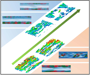
Characteristic flow structures are essential kernels for the maintenance of turbulence, through which the different dynamics (IT-related or EIT-related) can be well identified. As mentioned in the introduction, viscoelastic EIT is featured by the emergence of trains of small-scale spanwise vortex structures with alternating signs that appear on elongated sheets of highly stretched polymers in the streamwise direction with a small upward tilt. With regard to Newtonian IT, coherent structures involve velocity streaks, quasi-streamwise vortices and hairpin vortices. Figures 17 and 18 show three-dimensional structures of  $Q=-\frac {1}{2}\partial _iu_j \partial _ju_i$ (the second invariant of the velocity gradient tensor) and
 $u'$ in the lower half-channel in the Newtonian flow and in an active state with high flow drag of MDR flows at
 $Wi=30$ and
 $L^2=1000\unicode{x2013}40\,000$. For the Newtonian case, the channel is filled with low-speed streaks, and typical small-scale hairpin vortex structures are very active in the flow. The legs of these hairpin vortices are very close to the wall, and the heads bulge up as the low-speed streaks sweep up. At lower
 $L^2$ (1000 and 2000), hairpin vortex structures and twisted velocity streaks can also be detected. Under the modulation of polymers, they are raised towards the channel centre and their sizes are enlarged significantly. At higher
 $L^2$ (10 000 and 40 000), velocity streaks exist and hairpin vortices are replaced by cylindrical structures close to the wall. These cylindrical structures are mostly streamwise and spanwise at
 $L^2=10\,000$ and 40 000, respectively.
Structural features of instantaneous isosurfaces of  $Q$ of the MDR (
 $Wi=30$) at an active moment with high flow drag for different
 $L^2$. Here
 $Q$ is the second invariant of the velocity gradient tensor.

Structural features of instantaneous isosurfaces of  $u'$ of the MDR
 $(Wi=30)$ at an active moment with high flow drag for different
 $L^2$

Figures 19 and 20 illustrate two-dimensional (2-D) snapshots of a polymer extension ( ${\rm tr}(\boldsymbol {C})=\sqrt {C_{ii}}$) superposed by
 $Q$ and
 $G$ in a
 $x$–
 $y$ section in an active state with high flow drag of the MDR flows at
 $Wi=30$ and
 $L^2=1000\sim 40\,000$, respectively, where
 $Q=(-1/2\partial _{i}u_{j}\partial _{j}u_{i})$ is the second invariant of the velocity gradient tensor. Under the conditions of lower
 $L^2$ (e.g.
 $L^2=1000\unicode{x2013}40\,000$), there are also high extension structures of polymers. These structures are overall distributed randomly, although they also have the trend of stretching along the streamwise direction. Many structures of
 $Q$ and
 $G$ are distributed randomly with the extension structures. The overall pattern therein looks like the extension structures of polymers that are passively induced due to IT-related dynamics. However, the pattern becomes very different when
 $L^2$ is raised to 10 000 and 40 000. The instantaneous extension fields display orderly sheet-like structures arranged along the streamwise direction and inclined toward the channel centre. Those structures seem qualitatively consistent with the chaotic arrowhead structures observed by Dubief et al. (Reference Dubief, Page, Kerswell, Terrapon and Steinberg2022) in their 2-D numerical simulation that may be originated from the centre mode. Here
 $G$ and
 $Q$ are alternately arranged along the extension sheets, indicating the appearance of the EIT mode. It is suggested that the orderly extension sheet becomes the key structure for turbulence maintenance at
 $L^2=10\,000$ and 40 000.
Structural features of the MDR regime in the  $x$–
 $y$ plane at an active moment with high flow drag for different
 $L^2$. The contour illustrates the distribution of the polymer extension (
 ${\rm tr}({\boldsymbol {C}})=\sqrt {C_{ii}}$). The superimposed lines illustrate the features of the vortex structures described by
 $Q$ and the energy transfer between the turbulence and the polymers described by
 $G$.

Structural features of the MDR regime in the  $x$–
 $y$ plane at a smooth moment with low flow drag for different
 $L^2$. The contour illustrates the distribution of the polymer extension (
 ${\rm tr}({\boldsymbol {C}})=\sqrt {C_{ii}}$). The superimposed lines illustrate the features of the vortex structures described by
 $Q$ and the energy transfer between the turbulence and the polymers described by
 $G$.

The above observations fully demonstrate that MDR flows at low  $L^2$ are dominated by IT-related dynamics, while EIT dynamics get involved at high
 $L^2$. Therefore, we argue that the MDR state for small and large
 $L^2$ has a different flow nature, and the nonlinear extension (
 $L^2$) is a crucial parameter in this process.
4. Discussion
The essence of the MDR flow state has changed from being considered as the edge state of IT in the early days to being considered as the state of EIT. Although there are still some disputes, the current state of EIT is becoming the prevailing view. However, the numerical results in the present paper show that unlike the previous conclusions that the MDR state has only one type of dominant dynamics, i.e. either the edge state of IT or the flow state of EIT, both the edge state of IT and the flow state of EIT are possible to be the essence of the MDR state where the nonlinear extension ( $L^2$) effect plays a key role in determining the dominant dynamics. According to the above results, for the cases of smaller
 $L^2$ with the stronger nonlinear extension (
 $L^2\leqslant 5000$ in this paper), the viscoelastic fluid flow shows the IT-related properties when the flow enters the MDR state, suggesting that it is still dominated by IT-related dynamics. However, for large
 $L^2$ with weaker nonlinear stretch (
 $L^2\ge 10\,000$ in this paper), the viscoelastic fluid behaves with EIT-related characteristics when the flow enters the MDR flow state suggesting that EIT-related dynamics dominates in this case. Moreover, there exists a critical stretch length
 $L^2$ (
 $L^2 = 5000$ in this paper). Under
 $L^2_c$, although not completely laminarized, the viscoelastic turbulent flow can reach the lowest turbulent drag resistance and breaks through the well-known Virk's MDR limit. It indicates that the proper choice of polymer additives is also important to achieve larger DR. On the basis of the above results, the following question naturally comes to mind: why does the nonlinear extension
 $L^2$ (the maximum stretching length of the molecule) have the above effects on the nature of the MDR regime? In the following we attempt to answer the above question from two aspects: the effective elasticity in viscoelastic DRT with different
 $L^2$ and the
 $L^2$ effect on the excitation of EIT.
As for the effective elasticity, since there exists a limit of the polymer extension for the FENE-P model, the effective elasticity felt by the flow will saturate when the polymer extension approaches its maximum extension no matter how large Wi is. In this aspect, the commonly used Wi that neglects the nonlinear extension effect and the variation of the local velocity gradient cannot reflect the above effect for FENE-P fluids. Taking the Oldroyd-B model ( $L^2 = \infty$) as a reference, the nonlinear extension effect on Wi can be mimicked as the modification of the polymer relaxation time. Hence, considering the effects of both nonlinear extension and the local shear, we define a local Wi to analyse the effective elasticity for different cases as
 \begin{equation} {{Wi}_{loc}=\frac{Wi}{{f^2(r)}} \frac{{{\rm d}U}}{{{\rm d} y}}}. \end{equation}
It also corresponds to the shear deformation induced by the local shear considering the nonlinear extension effect for the base flow, i.e. the component  $C_{xy}$ of the conformation tensor
 ${\boldsymbol {c}}^B$ in (3.2). Compared with the Oldroyd-B model, the FENE-P model considers the nonlinear extension of molecules that brings about the effect of actual Wi reduction with the molecular structure stretching. In our previous study for the Oldroyd-B model, the EIT-related dynamics have come into play when the mean
 $Wi\geqslant 8$. Due to the nonlinear extension effect of the FENE-P model at the same mean Wi, the smaller
 $L^2$, the smaller the actual Wi felt by the flow, and it tends to be saturated with an increase of Wi. Taking the laminar flow as a reference, we compare the local Wi distribution of the FENE-P model under different
 $L^2$ and Wi, as shown in figures 21 and 22. It can be seen that due to the nonlinear extension effect, the local Wi saturates in the investigated Wi range for the cases of smaller
 $L^2$ indicating that the saturation of the effective elasticity felt by the flow, while the effective elasticity keeps increasing with Wi that will never saturate or converge for high
 $L^2$ case and especially the Oldroyd-B model. For example,
 $Wi_{local}$ saturates around 11 and 16 for
 $L^2 = 1000$ and
 $L^2 = 2000$, respectively. Moreover, for the cases of large
 $L^2$ (e.g.
 $L^2 = 10\,000$ or 40 000), the local Wi near the wall can be significantly higher than that of the small
 $L^2$ (e.g.
 $L^2 = 1000$) even at much smaller Wi. Under the combination of this effect, the larger
 $L^2$ has a more effective elastic effect in the near-wall region even at lower Wi, resulting in a larger elastic stress and a dominant effect on the flow. As illustrated in figure 21(b), it can be seen that
 $L^2 =10\,000$ and 40 000 have produced much larger elastic stress in the near-wall region even at
 $Wi= 5$ than
 $L^2 =1000$ and 2000 at
 $Wi=30$. At
 $Wi = 8$, the elastic stress of the cases of
 $L^2 =10\,000$ and 40 000 is greater than that of the cases of
 $L^2 =1000$ and 2000 at
 $Wi = 30$ in the whole channel. Therefore, the larger
 $L^2$ introduces more effective elasticity in the viscoelastic turbulence at fixed Wi.
Local Wi distribution with Wi under different  $L^2$: (a)
 $L^2=1000$, (b)
 $L^2=2000$, (c)
 $L^2=10\,000$, (d)
 $L^2=40\,000$.

(a) Local Wi distribution of the MDR state at different  $L^2$. (b) Distributions of the nonlinear part of the elastic shear stress induced by the interaction between microstuctures and turbulence.

From the above results, we speculate that the nonlinear extension of polymers has an inhibitory effect on the effective elasticity of viscoelastic fluid. The smaller  $L^2$ is, the smaller the effective elasticity felt by the flow, and the less likely the EIT is excited. In addition, Sid et al. (Reference Sid, Terrapon and Dubief2018) demonstrated the 2-D nature of EIT. In order to prove the above speculation, we carry out DNS of a 2-D turbulent channel flow to remove the effect of the IT-related dynamics. The specific calculation parameters are similar to those of three-dimensional DNS, except that the spanwise effect is ignored. Figure 23 shows instantaneous contours of polymer extension superimposed with contour lines of
 $v'$ when the turbulence is active at
 $Wi=20$ obtained based on 2-D DNS. Here, we reproduce the flow pattern of EIT, through comparing polymer extension structures reported by Shekar et al. (Reference Shekar, McMullen, McKeon and Graham2021) and Dubief et al. (Reference Dubief, Page, Kerswell, Terrapon and Steinberg2022). To judge whether elasto-inertia instability (EII) and turbulence occur, the 2-D DNS results show that EII can exist when
 $Wi > 3$ or 4, and the EIT phenomenon occurs when Wi is further increased under the given Re and
 $\beta$ for the Oldroyd-B model. For the FENE-P model at
 $L^2=10\,000$ or 40 000, when
 $Wi > 5\unicode{x2013}6$, the flow becomes unstable, and the EIT phenomenon occurs when Wi is further increased. At
 $L^2 = 1000$ or 2000, the flow remains stable until Wi reaches 60 or 30, respectively. The above results demonstrate that EII and EIT are more difficult to achieve for small
 $L^2$. In other words, the nonlinear extension of polymers can somehow inhibit the EII and EIT to a certain extent. Based on this, we can explain the phenomenon observed above. The elastic nonlinear extension of polymers has two effects on DRT. With an increase of
 $L^2$ (the degree of elastic nonlinear extension decreases), the stronger inhibition effect on IT by polymers, the more likely the EIT is excited. Correspondingly, the flow essence of MDR gradually changes from the IT modulated by polymers to the coexistence state of IT and EIT until it is completely replaced by EIT with an increase of
 $L^2$.
Structural characteristics of the velocity field and polymer extension of viscoelastic fluid flow under different  $L^2$ conditions at
 $Wi=20$ obtained by 2-D numerical simulation.

5. Concluding remarks
In summary, although EIT has been proven to have a dominant role in the feature and dynamics of the MDR state, the essence of the MDR state, either EIT or inertia-driven turbulence (IDT), has not been pinned down as many important parametric effects are still unknown and in lack of systematic research. In particular, no relevant research on the effect of nonlinear extension on the nature of MDR has been conducted among the existing literature. To this end, a large number of DNS of DRT at modest Reynolds number Re with  $Re = 6000$ for the FENE-P model are conducted, covering a wide range of flow states and nonlinear extension effects on statistical properties, energy spectrum, characteristic structures and underlying dynamics especially in the MDR state are investigated by varying
 $L^2$. The following conclusions can be obtained.
(1) Variation of the nonlinear extension can modulate the thresholds and ranges that a viscoelastic turbulent flow enters different states. In general, the flow with larger
 $L^2$ enter MDR at a lower Wi. It is interesting that before and after entering MDR, nonlinear extension effects show different laws for small and large $L^2$. Before entering the MDR state, the effect of increasing $L^2$ on the flow characteristics shows a monotonic trend to the flow pattern with smaller drag. However, a non-monotonic effect of increasing $L^2$ on the flow pattern can be observed with a critical $L_c^2$, corresponding to the lowest flow drag even breaking through Virk's MDR limit after entering the MDR state. For the cases that on two sides of $L_c^2$ the flow in the MDR state shows completely different scaling relations imply different dominant scenarios that are possibly IT-related dynamics dominant for cases of small $L^2$ but EIT-related dynamics dominant for cases of large $L^2$.
(2) Further analyses on the stress balance, energy spectrum, characteristic structures and the underlying dynamics also supports this argument that the MDR state can be dominated by both IDT-related and EIT-related dynamical cycles, but which dynamics dominates is closely related to the nonlinear extension effect
$L^2$. In other words, the proper choice of the polymer length and concentration of polymer additives is helpful to reach a better DR effect.(3) To explain the above observation, an effective elasticity is introduced by defining a local Wi and
$L^2$ effects on the excitation of pure EIT on 2-D DNS. It indicates that the smaller $L^2$ is (when polymers have stronger nonlinear extension), the less effective the elastic effect actually introduced is. Moreover, it is also found that EIT is more difficult to be excited for the case of smaller $L^2$. Therefore, the reason that the MDR state behaves like IT dominant features for the case of small $L^2$ can be qualitatively explained as: IT cannot be fully eliminated due to the fact that relatively less effective elasticity is introduced, and EIT is not also excited due to the saturation of the effective elasticity. In contrast, for the case of large $L^2$, EIT can be excited before complete suppression of IT-related features.


Author contributions
Suming Wang and Wenhua Zhang contributed equally to this work and are recognized as joint first authors.
Funding
This research was funded by the National Natural Science Foundation of China (NSFC 51976238, 12202308, 52176160).
Declaration of interests
The authors report no conflict of interest.



