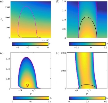
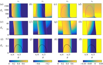
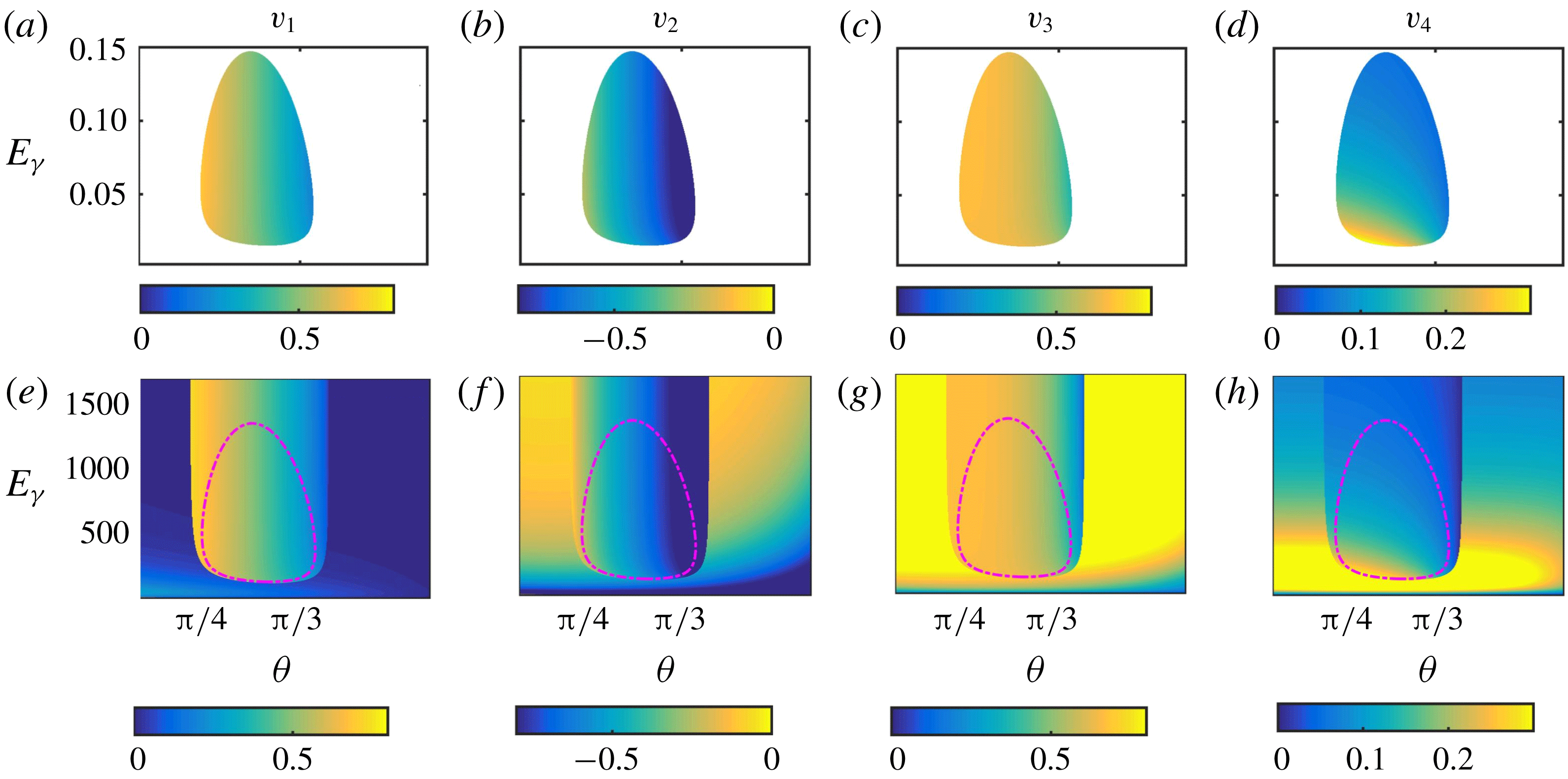
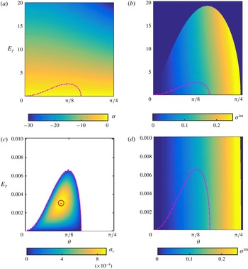
1 Introduction
Small-scale linear instabilities on vortices are often observed in a wide variety of engineering (Spalart Reference Spalart1998) and natural flows (Carton Reference Carton2001). These short-wavelength instabilities are a mechanism by which three-dimensional features arise in large-scale two-dimensional flows (Pierrehumbert & Widnall Reference Pierrehumbert and Widnall1982; Orszag & Patera Reference Orszag and Patera1983; Corcos & Lin Reference Corcos and Lin1984; Metcalfe et al. Reference Metcalfe, Orszag, Brachet, Menon and Riley1987). A local approach, which calculates the inviscid evolution of relatively short-wavelength perturbations on two-dimensional, elliptical vortex core regions, was hence developed to understand the universality of vortex breakdown characteristics across various flows (Bayly Reference Bayly1986; Pierrehumbert Reference Pierrehumbert1986). The general local stability equations that govern the inviscid evolution of three-dimensional, short-wavelength, small-amplitude perturbations on any base flow are attributed to Lifschitz & Hameiri (Reference Lifschitz and Hameiri1991). In this paper, we use the local stability approach to study axisymmetric and non-axisymmetric planar vortices with an out-of-plane stable stratification, and gravity acting along the vorticity axis. These stratified vortices represent an idealized model of geophysical settings such as eddies in the salinity/temperature-stratified ocean and hurricanes in the temperature-stratified atmosphere.
The elliptic instability is now recognized as a consequence of parametric resonance between the normal mode of the undistorted rotating flow and the underlying strain field (Kerswell Reference Kerswell2002). In purely elliptical flow, the local stability equations uncover the elliptic instability for the wave vector inclined at an angle
 $\unicode[STIX]{x03C0}/3$
with respect to the vorticity axis of the flow. The local stability approach has also shed light on centrifugal (Bayly Reference Bayly1988) and hyperbolic (Leblanc Reference Leblanc1997) instabilities. Subsequent inviscid studies based on the local approach have then investigated the role of one or more of various factors such as multipolar strain field, background rotation and axial flow on the elliptic, centrifugal and hyperbolic instabilities (Le Dizes & Eloy Reference Le Dizes and Eloy1999; Le Dizès Reference Le Dizès2000; Sipp & Jacquin Reference Sipp and Jacquin2000; Godeferd, Cambon & Leblanc Reference Godeferd, Cambon and Leblanc2001; Mathur et al.
Reference Mathur, Ortiz, Dubos and Chomaz2014; Nagarathinam, Sameen & Mathur Reference Nagarathinam, Sameen and Mathur2015). Landman & Saffman (Reference Landman and Saffman1987) considered the viscous terms in the local stability approach, and showed via a transformation introduced by Craik & Criminale (Reference Craik and Criminale1986) that weak viscous effects serve only to suppress the inviscid growth rates. Landman & Saffman (Reference Landman and Saffman1987) proceeded to calculate the threshold perturbation wavenumbers below which three-dimensional, inviscid instabilities persist in viscous, elliptical flows. Similar viscous corrections, along with finite-wavenumber corrections introduced by Bayly (Reference Bayly1988), have led to improved agreement between the local and global approaches in numerically simulated vortical wake flows behind bluff bodies (Gallaire, Marquillie & Ehrenstein Reference Gallaire, Marquillie and Ehrenstein2007; Jethani et al.
Reference Jethani, Kumar, Sameen and Mathur2018).
Miyazaki & Fukumoto (Reference Miyazaki and Fukumoto1992) included buoyancy effects in the local stability equations, and studied the effects of an out-of-plane stable stratification (stratification/buoyancy along the vorticity axis) on the inviscid local instabilities in an elliptical vortex. Apart from the suppression of the elliptic instability at some threshold stratification, new instabilities were shown to emerge at even stronger stratifications. Subsequent studies by Miyazaki (Reference Miyazaki1993) investigated the simultaneous presence of out-of-plane stable stratification and background rotation in an elliptical vortex. Recently, Aravind, Mathur & Dubos (Reference Aravind, Mathur and Dubos2017) have used the local approach to study the inviscid instabilities in stratified Kelvin–Helmholtz vortices, where the density gradients (gravitationally stable or unstable) occur in the same plane as the vortex, i.e. in-plane buoyancy. It is noteworthy that the conclusion that viscous effects serve only to suppress inviscid instabilities (Landman & Saffman Reference Landman and Saffman1987) does not necessarily extend to the case of unequal diffusivities in the momentum and buoyancy equations. Indeed, numerical simulations and global mode stability calculations on stratified Kelvin–Helmholtz vortices have highlighted the significant role of Prandtl number in their instability characteristics and flow evolution (Klaassen & Peltier Reference Klaassen and Peltier1985; Cortesi, Yadigaroglu & Banerjee Reference Cortesi, Yadigaroglu and Banerjee1998).
Kirillov & Mutabazi (Reference Kirillov and Mutabazi2017) incorporated the effects of buoyancy diffusion in the local stability equations, assuming both the kinematic viscosity
 $\unicode[STIX]{x1D708}$
and the thermal diffusivity
 $\unicode[STIX]{x1D705}$
to be small, to study the effects of Prandtl number (
 $Pr=\unicode[STIX]{x1D708}/\unicode[STIX]{x1D705}$
) on the instabilities in the axisymmetric flow in between rotating concentric cylinders that are differentially heated. In this study by Kirillov & Mutabazi (Reference Kirillov and Mutabazi2017), there was no gravity, and the (in-plane) radial buoyancy results from retaining density variations in the centrifugal terms of the momentum equations. They find significant effects of radial buoyancy and Prandtl number on both the centrifugally unstable and stable regimes. In the centrifugally unstable flow, radial heating, depending on its sign, either enhances the instability or induces oscillatory modes of instability whose frequencies depend on
 $Pr$
. In the centrifugally stable flow, large and small values of
 $Pr$
were respectively shown to induce instabilities in the form of stationary and oscillatory modes if a radial heating with the appropriate sign is added. In this paper, we investigate the effects of Prandtl number (its role played by the Schmidt number
 $Sc$
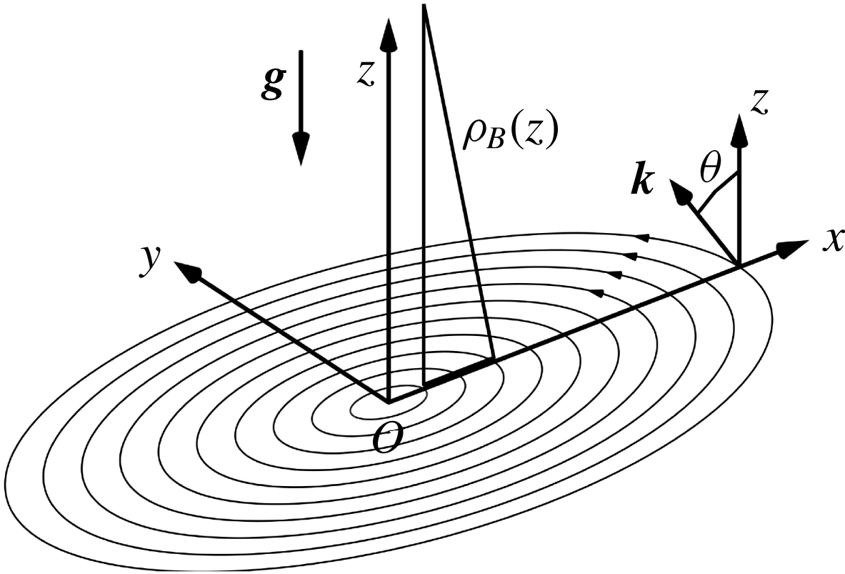
defined in § 2 in this paper) too, but on axisymmetric and non-axisymmetric vortices with an out-of-plane stable stratification and no in-plane stratification, with gravity along the vorticity axis. A schematic of the base flow we consider is shown in figure 1. To the best of our knowledge, no previous study based on the local stability approach has investigated the effects of
 $Pr$
(or
 $Sc$
) on vortex instabilities, in axisymmetric or non-axisymmetric vortices in the presence of an out-of-plane stable stratification.
Schematic of the base flow and perturbation wave vector orientation. The base flow field is described by a streamfunction
 $\unicode[STIX]{x1D713}(x,y)$
, and a stable stratification
 $\unicode[STIX]{x1D70C}_{B}(z)$
. The gravity vector is given by
 $\boldsymbol{g}=-g\hat{\boldsymbol{e}}_{z}$
, with
 $g>0$
. A sample initial perturbation wave vector
 $\boldsymbol{k}$
and the angle
 $\unicode[STIX]{x1D703}$
it makes with the
 $z$
-axis are also shown. The local stability equations are solved on the closed streamlines in the
 $x$
–
 $y$
plane to obtain growth rates for all periodic wave vectors.

Diffusive instabilities resulting from
 $Pr\neq 1$
have been reported in other flows as well. McIntyre (Reference McIntyre1970) used the normal mode approach to investigate axisymmetric zonal flow (azimuthal flow in the
 $x$
–
 $y$
plane) in the presence of background rotation (along
 $z$
), out-of-plane stable stratification (along the gravity direction
 $z$
), and in-plane (
 $x$
–
 $y$
plane) density variations that are related to the out-of-plane velocity gradients for thermal wind balance; unlike Kirillov & Mutabazi (Reference Kirillov and Mutabazi2017), centrifugal buoyancy was ignored by McIntyre (Reference McIntyre1970). McIntyre (Reference McIntyre1970) showed that the further away from unity
 $Pr$
is, the larger is the parameter range (describing the base flow and the perturbation wave vector) for which normal mode instabilities exist. This diffusive destabilization resulting from
 $Pr\neq 1$
has been observed in laboratory experiments (Baker Reference Baker1971; Meunier, Miquel & Le Dizès Reference Meunier, Miquel, Le Dizès, Chowdhury and Alam2014), normal mode analysis of pancake vortices (Yim & Billant Reference Yim and Billant2016), and is thought to be a mechanism by which density layering occurs in oceanic eddies (Calman Reference Calman1977).
The present study based on the local stability approach does not include background rotation, and is distinct from the normal mode study of McIntyre (Reference McIntyre1970), with our base flow containing no in-plane stratification and no vertical momentum gradient. Even in the axisymmetric limit, our current study focuses more on the centrifugally unstable regime, whereas McIntyre (Reference McIntyre1970) restricted their study to the centrifugally stable regime. Other normal mode and numerical studies have investigated instabilities on axisymmetric (Riedinger, Le Dizès & Meunier Reference Riedinger, Le Dizès and Meunier2010) and non-axisymmetric (Waite & Smolarkiewicz Reference Waite and Smolarkiewicz2008) planar vortices with an out-of-plane stratification and specific
 $Sc$
values greater than unity, but do not isolate the effects of
 $Sc\neq 1$
. In summary, the role of
 $Sc$
in the instabilities of axisymmetric or non-axisymmetric vortices in the presence of an out-of-plane stable stratification is not well understood.
We present the local stability equations with diffusive terms in both the momentum and buoyancy equations in § 2, followed by a brief discussion of the numerical method used to obtain instability growth rates. Axisymmetric and elliptical vortices are considered in §§ 3 and 4, respectively, followed by an analysis of hyperbolic instability in § 5. We summarize our results in § 6, followed by a discussion of potential applications of our results and the scope for further follow-up studies.
2 Theory and methods
We consider small perturbations (denoted by superscript
 $^{\prime }$
) superimposed on a base flow (denoted by subscript
 $B$
) so that the net flow is described by
 $$\begin{eqnarray}\boldsymbol{u}=\boldsymbol{u}_{B}+\boldsymbol{u}^{\prime },\quad p=p\!_{B}+p^{\prime },\quad \unicode[STIX]{x1D70C}=\unicode[STIX]{x1D70C}_{B}+\unicode[STIX]{x1D70C}^{\prime },\end{eqnarray}$$
where
 $\boldsymbol{u},p$
and
 $\unicode[STIX]{x1D70C}$
are the net velocity, pressure and density fields, respectively. The linearized equations (within the incompressible, Boussinesq approximations) governing the perturbation quantities are
 $$\begin{eqnarray}\displaystyle & \displaystyle \unicode[STIX]{x1D735}\boldsymbol{\cdot }\boldsymbol{u}^{\prime }=0, & \displaystyle\end{eqnarray}$$
 $$\begin{eqnarray}\displaystyle & \displaystyle {\displaystyle \frac{\text{d}\boldsymbol{u}^{\prime }}{\text{d}t}}+\unicode[STIX]{x1D735}\boldsymbol{u}_{B}\boldsymbol{\cdot }\boldsymbol{u}^{\prime }+\unicode[STIX]{x1D735}p^{\prime }=\unicode[STIX]{x1D708}\unicode[STIX]{x1D6FB}^{2}\boldsymbol{u}^{\prime }+b^{\prime }\boldsymbol{e}_{\boldsymbol{g}}, & \displaystyle\end{eqnarray}$$
 $$\begin{eqnarray}\displaystyle & \displaystyle {\displaystyle \frac{\text{d}b^{\prime }}{\text{d}t}}+\boldsymbol{u}^{\prime }\boldsymbol{\cdot }\unicode[STIX]{x1D735}\unicode[STIX]{x1D70C}_{B}{\displaystyle \frac{g}{\unicode[STIX]{x1D70C}_{o}}}=\unicode[STIX]{x1D705}\unicode[STIX]{x1D6FB}^{2}b^{\prime }, & \displaystyle\end{eqnarray}$$
where
 $t$
is time,
 $b^{\prime }=\unicode[STIX]{x1D70C}^{\prime }g/\unicode[STIX]{x1D70C}_{o}$
is the perturbation buoyancy,
 $\boldsymbol{g}=g\boldsymbol{e}_{\boldsymbol{g}}$
is the acceleration due to gravity acting along unit vector
 $\boldsymbol{e}_{\boldsymbol{g}}$
with
 $g>0$
,
 $\unicode[STIX]{x1D70C}_{o}$
a constant reference density, and
 $\unicode[STIX]{x1D708}$
and
 $\unicode[STIX]{x1D705}$
the diffusivity of momentum and density, respectively. Here,
 $\text{d}/\text{d}t$
is the material time derivative in the base flow, which is assumed to satisfy the incompressible Navier–Stokes equations in the Boussinesq approximation. Within the local stability framework (Lifschitz & Hameiri Reference Lifschitz and Hameiri1991), we assume perturbations of the form
 $$\begin{eqnarray}\displaystyle & \displaystyle \boldsymbol{u}^{\prime }=\exp (\text{i}\unicode[STIX]{x1D719}(\boldsymbol{x},t)/\unicode[STIX]{x1D6FF})[\boldsymbol{a}(\boldsymbol{x},t)+\unicode[STIX]{x1D6FF}\boldsymbol{a}_{\unicode[STIX]{x1D6FF}}(\boldsymbol{x},t)+\cdots \,], & \displaystyle\end{eqnarray}$$
 $$\begin{eqnarray}\displaystyle & \displaystyle p^{\prime }=\exp (\text{i}\unicode[STIX]{x1D719}(\boldsymbol{x},t)/\unicode[STIX]{x1D6FF})[\unicode[STIX]{x03C0}(\boldsymbol{x},t)+\unicode[STIX]{x1D6FF}\unicode[STIX]{x03C0}_{\unicode[STIX]{x1D6FF}}(\boldsymbol{x},t)+\cdots \,], & \displaystyle\end{eqnarray}$$
 $$\begin{eqnarray}\displaystyle & \displaystyle b^{\prime }=\exp (\text{i}\unicode[STIX]{x1D719}(\boldsymbol{x},t)/\unicode[STIX]{x1D6FF})[b(\boldsymbol{x},t)+\unicode[STIX]{x1D6FF}b_{\unicode[STIX]{x1D6FF}}(\boldsymbol{x},t)+\cdots \,], & \displaystyle\end{eqnarray}$$
where
 $\unicode[STIX]{x1D6FF}$
is a small parameter. The wave vector of the perturbations is
 $\boldsymbol{k}^{\prime }=\unicode[STIX]{x1D735}\unicode[STIX]{x1D719}/\unicode[STIX]{x1D6FF}=\boldsymbol{k}/\unicode[STIX]{x1D6FF}$
, thus rendering the analysis relevant only for short-wavelength perturbations. Here,
 $\unicode[STIX]{x1D719}$
is a real scalar field, and (
 $\boldsymbol{a},\unicode[STIX]{x03C0},b$
) are the complex leading-order amplitudes for the velocity, pressure and buoyancy perturbations, respectively. The expressions in (2.5)–(2.7) are substituted in the linearized governing equations (2.2)–(2.4) to obtain the evolution equations for
 $\boldsymbol{k}$
,
 $\boldsymbol{a}$
and
 $b$
as
 $$\begin{eqnarray}\displaystyle & \displaystyle \boldsymbol{a}\boldsymbol{\cdot }\boldsymbol{k}=0, & \displaystyle\end{eqnarray}$$
 $$\begin{eqnarray}\displaystyle & \displaystyle {\displaystyle \frac{\text{d}\boldsymbol{k}}{\text{d}t}}=(\unicode[STIX]{x1D735}\times \boldsymbol{u}_{B})\times \boldsymbol{k}-(\boldsymbol{k}\boldsymbol{\cdot }\unicode[STIX]{x1D735})\boldsymbol{u}_{B}, & \displaystyle\end{eqnarray}$$
 $$\begin{eqnarray}\displaystyle & \displaystyle {\displaystyle \frac{\text{d}\boldsymbol{a}}{\text{d}t}}=-\unicode[STIX]{x1D735}\boldsymbol{u}_{B}\boldsymbol{\cdot }\boldsymbol{a}+b\boldsymbol{e}_{\boldsymbol{g}}+{\displaystyle \frac{\boldsymbol{k}}{|\boldsymbol{k}|^{2}}}[2(\unicode[STIX]{x1D735}\boldsymbol{u}_{B}\boldsymbol{\cdot }\boldsymbol{a})\boldsymbol{\cdot }\boldsymbol{k}-b\boldsymbol{e}_{\boldsymbol{g}}\boldsymbol{\cdot }\boldsymbol{k}]-c_{\unicode[STIX]{x1D708}}|\boldsymbol{k}|^{2}\boldsymbol{a}, & \displaystyle\end{eqnarray}$$
 $$\begin{eqnarray}\displaystyle & \displaystyle {\displaystyle \frac{\text{d}b}{\text{d}t}}=-(\boldsymbol{a}\boldsymbol{\cdot }\unicode[STIX]{x1D735}\unicode[STIX]{x1D70C}_{B}){\displaystyle \frac{g}{\unicode[STIX]{x1D70C}_{o}}}-c_{\unicode[STIX]{x1D705}}|\boldsymbol{k}|^{2}b, & \displaystyle\end{eqnarray}$$
where the diffusivities
 $\unicode[STIX]{x1D708}$
and
 $\unicode[STIX]{x1D705}$
are assumed to be of
 $\mathit{O}(\unicode[STIX]{x1D6FF}^{2})$
, i.e.
 $\unicode[STIX]{x1D708}=c_{\unicode[STIX]{x1D708}}\unicode[STIX]{x1D6FF}^{2}$
and
 $\unicode[STIX]{x1D705}=c_{\unicode[STIX]{x1D705}}\unicode[STIX]{x1D6FF}^{2}$
with
 $c_{\unicode[STIX]{x1D708}}$
and
 $c_{\unicode[STIX]{x1D705}}$
being positive constants. The corresponding Schmidt number is
 $Sc=\unicode[STIX]{x1D708}/\unicode[STIX]{x1D705}=c_{\unicode[STIX]{x1D708}}/c_{\unicode[STIX]{x1D705}}$
. The assumption of
 $\unicode[STIX]{x1D708}\sim \unicode[STIX]{x1D6FF}^{2}$
prevents rapid viscous decay of short-wavelength perturbations, and has previously been used indirectly in local stability studies with a single diffusivity, i.e. no buoyancy effects (Landman & Saffman Reference Landman and Saffman1987; Gallaire et al.
Reference Gallaire, Marquillie and Ehrenstein2007). Recently, the local stability analysis of Kirillov & Mutabazi (Reference Kirillov and Mutabazi2017) successfully derived instability criteria in axisymmetric flows with in-plane radial buoyancy by assuming both momentum and buoyancy diffusivities to be proportional to
 $\unicode[STIX]{x1D6FF}^{2}$
.
Equations (2.9)–(2.10), in the limit of
 $\unicode[STIX]{x1D70C}_{B}=\unicode[STIX]{x1D70C}_{o}$
,
 $b=0$
,
 $c_{\unicode[STIX]{x1D708}}=0$
, reduce to what appears in Lifschitz & Hameiri (Reference Lifschitz and Hameiri1991). The effect of viscosity in (2.9)–(2.10) was studied by Landman & Saffman (Reference Landman and Saffman1987) in the context of a simple elliptical vortex with no buoyancy (
 $\unicode[STIX]{x1D70C}_{B}=\unicode[STIX]{x1D70C}_{o},b=0,c_{\unicode[STIX]{x1D708}}\neq 0$
). Miyazaki & Fukumoto (Reference Miyazaki and Fukumoto1992) considered equations (2.9)–(2.11) with
 $c_{\unicode[STIX]{x1D708}}=c_{\unicode[STIX]{x1D705}}=0$
to investigate the effects of out-of-plane stable stratification on the stability of an elliptical vortex in the inviscid limit. Equations (2.9)–(2.11) with
 $c_{\unicode[STIX]{x1D708}}\neq 0$
and
 $c_{\unicode[STIX]{x1D705}}\neq 0$
were considered by Kirillov & Mutabazi (Reference Kirillov and Mutabazi2017) to investigate the effects of in-plane stratification produced by a radial temperature gradient in a circular (axisymmetric) Couette flow. Our current work concerns an investigation of (2.9)–(2.11) with
 $c_{\unicode[STIX]{x1D708}}\neq 0$
and
 $c_{\unicode[STIX]{x1D705}}\neq 0$
for a base flow described by planar axisymmetric and non-axisymmetric vortices with an out-of-plane stable stratification.
For a steady base flow described by a planar vortex in the
 $x$
–
 $y$
plane, i.e.
 $\boldsymbol{u}_{B}=-(\unicode[STIX]{x2202}\unicode[STIX]{x1D713}/\unicode[STIX]{x2202}y)\hat{\boldsymbol{e}}_{x}+(\unicode[STIX]{x2202}\unicode[STIX]{x1D713}/\unicode[STIX]{x2202}x)\hat{\boldsymbol{e}}_{y}$
(
 $\unicode[STIX]{x1D713}(x,y)$
is the streamfunction) with an out-of-plane stable stratification such that
 $\unicode[STIX]{x1D735}\unicode[STIX]{x1D70C}_{B}(z)=(\text{d}\unicode[STIX]{x1D70C}_{B}/\text{d}z)\hat{\boldsymbol{e}}_{z}$
and
 $\boldsymbol{e}_{\boldsymbol{g}}=-\hat{\boldsymbol{e}}_{z}$
, the governing equations (2.10)–(2.11) for the perturbation amplitudes reduce to
 $$\begin{eqnarray}\displaystyle & \displaystyle {\displaystyle \frac{\text{d}\boldsymbol{a}}{\text{d}t}}=-\unicode[STIX]{x1D735}\boldsymbol{u}_{B}\boldsymbol{\cdot }\boldsymbol{a}-b\hat{\boldsymbol{e}}_{z}+{\displaystyle \frac{\boldsymbol{k}}{|\boldsymbol{k}|^{2}}}[2(\unicode[STIX]{x1D735}\boldsymbol{u}_{B}\boldsymbol{\cdot }\boldsymbol{a})\boldsymbol{\cdot }\boldsymbol{k}+bk_{z}]-c_{\unicode[STIX]{x1D708}}|\boldsymbol{k}|^{2}\boldsymbol{a}, & \displaystyle\end{eqnarray}$$
 $$\begin{eqnarray}\displaystyle & \displaystyle {\displaystyle \frac{\text{d}b}{\text{d}t}}=a_{z}N^{2}-c_{\unicode[STIX]{x1D705}}|\boldsymbol{k}|^{2}b, & \displaystyle\end{eqnarray}$$
where
 $N=\sqrt{-(\text{d}\unicode[STIX]{x1D70C}_{B}/\text{d}z)(g/\unicode[STIX]{x1D70C}_{o})}$
is the constant Brunt–Väisälä frequency associated with the background stratification, and
 $\boldsymbol{k}=k_{x}\hat{\boldsymbol{e}}_{x}+k_{y}\hat{\boldsymbol{e}}_{y}+k_{z}\hat{\boldsymbol{e}}_{z}$
. We solve (2.12)–(2.13) on closed streamlines in the base flow for those wave vectors
 $\boldsymbol{k}$
that are periodic upon integrating equation (2.9) around the closed streamline (figure 1).
For every periodic wave vector
 $\boldsymbol{k}$
on a given closed streamline, we invoke Floquet theory to calculate the corresponding growth rate. The amplitude evolution equations (2.12)–(2.13) for periodic wave vectors on a closed streamline can be written as
 $\text{d}(\boldsymbol{a}|b)/\text{d}t=A(t)(\boldsymbol{a}|b)$
, where
 $A(t)$
is time-periodic with the same period
 $T$
as that of the closed streamline and the wave vector. Four linearly independent initial conditions for the vector
 $\boldsymbol{V}=(\boldsymbol{a}|b)$
are taken to be the columns of the initial condition matrix
 $\unicode[STIX]{x1D648}_{0}=I$
, where
 $I$
is the
 $4\times 4$
identity matrix. Equations (2.12)–(2.13) when integrated from
 $t=0$
to
 $T$
for the four different initial conditions in
 $\unicode[STIX]{x1D648}_{0}$
give the evolved amplitude vectors at
 $t=T$
, which are used as column vectors to construct the propagator matrix
 $\unicode[STIX]{x1D648}_{T}$
. The complex growth rate is then given by
 $\unicode[STIX]{x1D70E}^{complex}=\unicode[STIX]{x1D70E}+\text{i}\unicode[STIX]{x1D70E}^{\text{i}\text{m}}$
, with
 $$\begin{eqnarray}\unicode[STIX]{x1D70E}=(1/T)\max (\text{Re}(\log (\unicode[STIX]{x1D706}_{1-4}))),\end{eqnarray}$$
where
 $\unicode[STIX]{x1D706}_{1-4}$
are the eigenvalues of
 $\unicode[STIX]{x1D648}_{T}$
, and
 $\text{Re}$
denotes real part. The imaginary part,
 $\unicode[STIX]{x1D70E}^{\text{i}\text{m}}$
, of the complex growth rate is
 $\unicode[STIX]{x1D70E}^{\text{i}\text{m}}=(1/T)\text{Im}(\log (\unicode[STIX]{x1D706}_{m}))$
, where
 $\unicode[STIX]{x1D706}_{m}$
is the dominant eigenvalue corresponding to the growth rate
 $\unicode[STIX]{x1D70E}$
. While
 $\unicode[STIX]{x1D70E}>0$
corresponds to an instability for a given set of parameters, stable regions with
 $\unicode[STIX]{x1D70E}<0$
may also contain signatures of instabilities that occur at other parameter values. The eigenvector (of unit magnitude) corresponding to the dominant eigenvalue
 $\unicode[STIX]{x1D706}_{m}$
is denoted as
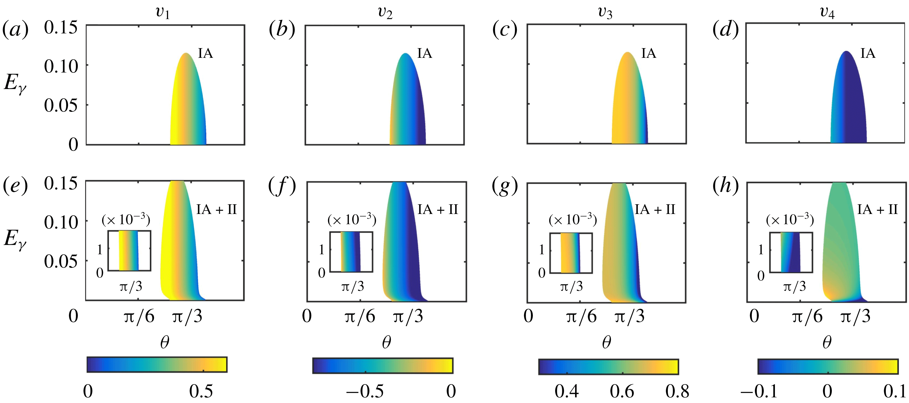
 $[v_{1},v_{2},v_{3},v_{4}]^{\text{T}}$
with
 $\text{Re}[v_{1}]\geqslant 0$
.
 $v_{1}$
,
 $v_{2}$
and
 $v_{3}$
are the components of the initial velocity perturbation amplitude and
 $v_{4}$
the initial buoyancy perturbation amplitude that correspond to the growth rate
 $\unicode[STIX]{x1D70E}$
. The structure of this eigenvector is used to distinguish between the various instabilities found numerically. The growth rate computation does not explicitly account for (2.8), which results from the mass conservation equation. In appendix A, we show that the perturbations with the growth rate
 $\unicode[STIX]{x1D70E}$
(2.14) indeed satisfy the constraint imposed by (2.8).
In the limit of
 $A(t)$
being invariant in time (like in § 3), the growth rate
 $\unicode[STIX]{x1D70E}$
coincides with the maximum real part of the eigenvalues of
 $A$
. For a time-dependent
 $A(t)$
, like in § 4 for the elliptical vortex, the growth rate
 $\unicode[STIX]{x1D70E}$
is calculated by numerically solving the local stability equations in cartesian coordinates for the aforementioned four linearly independent initial conditions using Runge–Kutta fourth-order integration in time. In certain regimes, particularly at small ellipticity (
 ${\sim}$
0.1),
 $\unicode[STIX]{x1D70E}$
tends to be of small magnitude and very sharply peaked when plotted as a function of
 $\unicode[STIX]{x1D703}$
, where
 $\unicode[STIX]{x1D703}$
is the angle made by the initial perturbation wave vector with the
 $z$
-axis (see figure 1). To ensure that sharp instability peaks are captured by the numerical solutions, we discretize the range
 $\unicode[STIX]{x1D703}\in [0,\unicode[STIX]{x03C0}/2]$
rad by approximately
 $2000$
points for moderate ellipticity (
 ${\sim}0.5$
), and by a significantly finer resolution of
 $\unicode[STIX]{x0394}\unicode[STIX]{x1D703}\approx 5\times 10^{-5}$
rad for small ellipticity. Furthermore, to ensure that the numerically obtained growth rates are not numerical artefacts, we verify that halving the time step does not change the growth rate magnitude by more than
 $1\,\%$
. In the next sections, we investigate base flows described by an axisymmetric vortex (§ 3), an elliptical vortex (§ 4) and the neighbourhood of a hyperbolic stagnation point (§ 5), with the goal of studying the effects of
 $Sc$
on centrifugal, elliptic and hyperbolic instabilities in isolation.
3 Results – axisymmetric vortex
To study the effects of out-of-plane stable stratification and Schmidt number on centrifugal instability, we consider an axisymmetric base flow described by
 $$\begin{eqnarray}\boldsymbol{u}_{B}=\dot{\unicode[STIX]{x1D713}}\hat{\boldsymbol{e}}_{q},\end{eqnarray}$$
where
 $\unicode[STIX]{x1D713}(r)$
is the streamfunction and
 $\dot{\unicode[STIX]{x1D713}}=\text{d}\unicode[STIX]{x1D713}/\text{d}r$
;
 $r$
and
 $q$
represent the radial and azimuthal coordinates in a cylindrical polar coordinate system on the
 $x$
–
 $y$
plane. As shown in Mathur et al. (Reference Mathur, Ortiz, Dubos and Chomaz2014), periodic wave vectors on a given circular streamline in this base flow are specified by
 $$\begin{eqnarray}\boldsymbol{k}=\unicode[STIX]{x1D6FD}\dot{\unicode[STIX]{x1D713}}\hat{\boldsymbol{e}}_{r}+k_{z}\hat{\boldsymbol{e}}_{z},\end{eqnarray}$$
where
 $\unicode[STIX]{x1D6FD}$
and
 $k_{z}$
are arbitrary constants, and hence
 $|\boldsymbol{k}|^{2}=\unicode[STIX]{x1D6FD}^{2}\dot{\unicode[STIX]{x1D713}}^{2}+k_{z}^{2}$
remains constant along the streamline. The angle
 $\unicode[STIX]{x1D703}$
made by
 $\boldsymbol{k}$
with the
 $z$
-axis is given by
 $\cos \unicode[STIX]{x1D703}=k_{z}/|\boldsymbol{k}|$
. Substituting the base flow (3.1) and periodic wave vector (3.2) expressions in (2.12)–(2.13), we obtain
 $$\begin{eqnarray}\left[{\displaystyle \frac{\text{d}a_{r}}{\text{d}t}},{\displaystyle \frac{\text{d}a_{q}}{\text{d}t}},{\displaystyle \frac{\text{d}a_{z}}{\text{d}t}},{\displaystyle \frac{\text{d}b}{\text{d}t}}\right]^{\text{T}}=\unicode[STIX]{x1D643}[a_{r},a_{q},a_{z},b]^{\text{T}},\end{eqnarray}$$
where
 $$\begin{eqnarray}\unicode[STIX]{x1D643}=\left(\begin{array}{@{}cccc@{}}-c_{\unicode[STIX]{x1D708}}|\boldsymbol{k}|^{2} & 2\left(1-{\displaystyle \frac{\unicode[STIX]{x1D6FD}^{2}\dot{\unicode[STIX]{x1D713}}^{2}}{|\boldsymbol{k}|^{2}}}\right){\displaystyle \frac{\dot{\unicode[STIX]{x1D713}}}{r}} & 0 & {\displaystyle \frac{k_{z}\unicode[STIX]{x1D6FD}\dot{\unicode[STIX]{x1D713}}}{|\boldsymbol{k}|^{2}}}\\ -\left(\ddot{\unicode[STIX]{x1D713}}+{\displaystyle \frac{\dot{\unicode[STIX]{x1D713}}}{r}}\right) & -c_{\unicode[STIX]{x1D708}}|\boldsymbol{k}|^{2} & 0 & 0\\ 0 & -2{\displaystyle \frac{k_{z}\unicode[STIX]{x1D6FD}\dot{\unicode[STIX]{x1D713}}}{|\boldsymbol{k}|^{2}}}{\displaystyle \frac{\dot{\unicode[STIX]{x1D713}}}{r}} & -c_{\unicode[STIX]{x1D708}}|\boldsymbol{k}|^{2} & -\left(1-{\displaystyle \frac{k_{z}^{2}}{|\boldsymbol{k}|^{2}}}\right)\\ 0 & 0 & N^{2} & -c_{\unicode[STIX]{x1D705}}|\boldsymbol{k}|^{2}\end{array}\right).\end{eqnarray}$$
With
 $\unicode[STIX]{x1D643}$
being time-invariant,
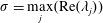 $\unicode[STIX]{x1D70E}=\underset{j}{\max }(\text{Re}(\unicode[STIX]{x1D706}_{j}))$
is the growth rate, where
 $\unicode[STIX]{x1D706}_{j}$
 $(1\leqslant j\leqslant 4)$
are the eigenvalues of
 $\unicode[STIX]{x1D643}$
. In the inviscid limit, i.e.
 $c_{\unicode[STIX]{x1D708}}=c_{\unicode[STIX]{x1D705}}=0$
, the eigenvalues of
 $\unicode[STIX]{x1D643}$
are governed by
 $$\begin{eqnarray}\unicode[STIX]{x1D706}^{2}\left[\unicode[STIX]{x1D706}^{2}+N^{2}\sin ^{2}\unicode[STIX]{x1D703}+2\cos ^{2}\unicode[STIX]{x1D703}{\displaystyle \frac{\dot{\unicode[STIX]{x1D713}}}{r}}\left(\ddot{\unicode[STIX]{x1D713}}+{\displaystyle \frac{\dot{\unicode[STIX]{x1D713}}}{r}}\right)\right]=0,\end{eqnarray}$$
the roots of which are
 $\unicode[STIX]{x1D706}_{1,2}=0$
and
 $$\begin{eqnarray}\unicode[STIX]{x1D706}_{3,4}=\pm \sqrt{-2\cos ^{2}\unicode[STIX]{x1D703}{\displaystyle \frac{\dot{\unicode[STIX]{x1D713}}}{r}}\left(\ddot{\unicode[STIX]{x1D713}}+{\displaystyle \frac{\dot{\unicode[STIX]{x1D713}}}{r}}\right)-N^{2}\sin ^{2}\unicode[STIX]{x1D703}}.\end{eqnarray}$$
The out-of-plane stable stratification
 $N$
thus reduces the inviscid growth rates associated with all the non-transverse wave vectors (
 $\unicode[STIX]{x1D703}\neq 0$
). The growth rate for purely transverse wave vectors (
 $\unicode[STIX]{x1D703}=0$
) is, however, unaffected by
 $N$
, resulting in the centrifugal instability criterion of
 $(\dot{\unicode[STIX]{x1D713}}/r)(\ddot{\unicode[STIX]{x1D713}}+\dot{\unicode[STIX]{x1D713}}/r)<0$
not being altered by stratification. Previous studies by Billant & Gallaire (Reference Billant and Gallaire2005) have also shown, using the normal mode approach in the limit of large axial wavenumbers, that out-of-plane stable stratification has no effect on the centrifugal instability criterion.
Returning to the viscous problem with
 $c_{\unicode[STIX]{x1D708}},c_{\unicode[STIX]{x1D705}}\neq 0$
, we define
 $\unicode[STIX]{x1D706}^{i}=\unicode[STIX]{x1D706}+c_{\unicode[STIX]{x1D708}}|\boldsymbol{k}|^{2}$
to write the governing equation for the eigenvalues of
 $\unicode[STIX]{x1D643}$
as
 $$\begin{eqnarray}\left|\begin{array}{@{}cccc@{}}-\unicode[STIX]{x1D706}^{i} & 2\left(1-{\displaystyle \frac{\unicode[STIX]{x1D6FD}^{2}\dot{\unicode[STIX]{x1D713}}^{2}}{|\boldsymbol{k}|^{2}}}\right){\displaystyle \frac{\dot{\unicode[STIX]{x1D713}}}{r}} & 0 & {\displaystyle \frac{k_{z}\unicode[STIX]{x1D6FD}\dot{\unicode[STIX]{x1D713}}}{|\boldsymbol{k}|^{2}}}\\ -\left(\ddot{\unicode[STIX]{x1D713}}+{\displaystyle \frac{\dot{\unicode[STIX]{x1D713}}}{r}}\right) & -\unicode[STIX]{x1D706}^{i} & 0 & 0\\ 0 & -2{\displaystyle \frac{k_{z}\unicode[STIX]{x1D6FD}\dot{\unicode[STIX]{x1D713}}}{|\boldsymbol{k}|^{2}}}{\displaystyle \frac{\dot{\unicode[STIX]{x1D713}}}{r}} & -\unicode[STIX]{x1D706}^{i} & -\left(1-{\displaystyle \frac{k_{z}^{2}}{|\boldsymbol{k}|^{2}}}\right)\\ 0 & 0 & N^{2} & (c_{\unicode[STIX]{x1D708}}-c_{\unicode[STIX]{x1D705}})|\boldsymbol{k}|^{2}-\unicode[STIX]{x1D706}^{i}\end{array}\right|=0.\end{eqnarray}$$
In the limit of
 $c_{\unicode[STIX]{x1D708}}=c_{\unicode[STIX]{x1D705}}$
, i.e.
 $Sc=1$
,
 $\unicode[STIX]{x1D706}^{i}$
coincides with the inviscid
 $(c_{\unicode[STIX]{x1D708}}=c_{\unicode[STIX]{x1D705}}=0)$
eigenvalues of
 $\unicode[STIX]{x1D643}$
. In other words, for
 $Sc=1$
, the viscous eigenvalues
 $\unicode[STIX]{x1D706}$
are given by the inviscid eigenvalues with a viscous correction given by
 $-c_{\unicode[STIX]{x1D708}}|\boldsymbol{k}|^{2}$
, a result that is similar to what is reported by Landman & Saffman (Reference Landman and Saffman1987) for elliptical vortices with no stratification.
For any
 $Sc>0$
,
 $\bar{\unicode[STIX]{x1D706}}^{i}=0$
is a trivial root of (3.7) and the other three roots are governed by
 $$\begin{eqnarray}(\bar{\unicode[STIX]{x1D706}}^{i})^{3}+(\bar{\unicode[STIX]{x1D706}}^{i})^{2}\left({\displaystyle \frac{1-Sc}{Sc}}\right)+\bar{\unicode[STIX]{x1D706}}^{i}[\unicode[STIX]{x1D6FC}_{1}+\unicode[STIX]{x1D6FC}_{2}]+\left({\displaystyle \frac{1-Sc}{Sc}}\right)\unicode[STIX]{x1D6FC}_{1}=0,\end{eqnarray}$$
where
 $$\begin{eqnarray}\unicode[STIX]{x1D6FC}_{1}={\displaystyle \frac{2k_{z}^{2}}{|\boldsymbol{k}|^{2}}}{\displaystyle \frac{1}{c_{\unicode[STIX]{x1D708}}^{2}|\boldsymbol{k}|^{4}}}{\displaystyle \frac{\dot{\unicode[STIX]{x1D713}}}{r}}\left(\ddot{\unicode[STIX]{x1D713}}+{\displaystyle \frac{\dot{\unicode[STIX]{x1D713}}}{r}}\right),\quad \unicode[STIX]{x1D6FC}_{2}={\displaystyle \frac{N^{2}}{c_{\unicode[STIX]{x1D708}}^{2}|\boldsymbol{k}|^{4}}}\left(1-{\displaystyle \frac{k_{z}^{2}}{|\boldsymbol{k}|^{2}}}\right),\end{eqnarray}$$
and
 $\bar{\unicode[STIX]{x1D706}}^{i}=\unicode[STIX]{x1D706}^{i}/(c_{\unicode[STIX]{x1D708}}|\boldsymbol{k}|^{2})=\unicode[STIX]{x1D706}/(c_{\unicode[STIX]{x1D708}}|\boldsymbol{k}|^{2})+1$
. We recall that instability occurs when at least one eigenvalue satisfies
 $\text{Re}(\unicode[STIX]{x1D706})>0$
, i.e.
 $\text{Re}(\bar{\unicode[STIX]{x1D706}})=\text{Re}(\bar{\unicode[STIX]{x1D706}}^{i}-1)>0$
, where
 $\bar{\unicode[STIX]{x1D706}}=\unicode[STIX]{x1D706}/(c_{\unicode[STIX]{x1D708}}|\boldsymbol{k}|^{2})$
. Equation (3.8) shows that the presence or absence of instability depends entirely on the values of three non-dimensional parameters, namely
 $\unicode[STIX]{x1D6FC}_{1}$
,
 $\unicode[STIX]{x1D6FC}_{2}$
(
 $\unicode[STIX]{x1D6FC}_{2}\geqslant 0$
for a stable stratification) and
 $Sc$
 $({>}0)$
. It is noteworthy that the criterion for inviscid centrifugal instability
 $\dot{\unicode[STIX]{x1D713}}(\ddot{\unicode[STIX]{x1D713}}+\dot{\unicode[STIX]{x1D713}}/r)<0$
can be written as
 $\unicode[STIX]{x1D6FC}_{1}<0$
. Physically,
 $\unicode[STIX]{x1D6FC}_{1}$
is a measure of the strength of the inviscid instability relative to the viscous effects, and
 $\unicode[STIX]{x1D6FC}_{2}$
quantifies the ratio between the stratification and viscous effects. Furthermore, as shown in appendix B, there exists no instability for
 $\unicode[STIX]{x1D6FC}_{1}>0$
with any
 $\unicode[STIX]{x1D6FC}_{2}>0$
,
 $Sc>0$
. In other words, an inviscidly stable axisymmetric vortex remains stable for any out-of-plane stable stratification (
 $N^{2}>0$
) with any
 $Sc>0$
. This is consistent with the results (based on the normal mode approach) of McIntyre (Reference McIntyre1970), who report that in the limit of zero vertical gradient for their base flow velocity and zero horizontal density gradient, a centrifugally stable vortex remains stable at all
 $Sc$
. We now proceed to explore the effects of
 $Sc$
on the instability of a centrifugally unstable (in the inviscid limit) vortex, i.e. the
 $\unicode[STIX]{x1D6FC}_{1}<0$
regime.
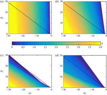
In figure 2, we plot
 $\bar{\unicode[STIX]{x1D70E}}=\max (\text{Re}(\bar{\unicode[STIX]{x1D706}}_{j}))$
,
 $1\leqslant j\leqslant 3$
by numerically solving equation (3.8) for various values of
 $\unicode[STIX]{x1D6FC}_{1},\unicode[STIX]{x1D6FC}_{2}$
and
 $Sc$
. In general,
 $\bar{\unicode[STIX]{x1D70E}}$
increases with
 $|\unicode[STIX]{x1D6FC}_{1}|$
, whereas it decreases with
 $|\unicode[STIX]{x1D6FC}_{2}|$
. In physical terms, an increase in
 $|\unicode[STIX]{x1D6FC}_{1}|$
enhances the inviscid centrifugal instability, whereas
 $\unicode[STIX]{x1D6FC}_{2}$
provides a stabilizing influence via the stable stratification. For
 $Sc=1$
, instability occurs if
 $\unicode[STIX]{x1D706}_{3}>c_{\unicode[STIX]{x1D708}}|\boldsymbol{k}|^{2}$
(
 $\unicode[STIX]{x1D706}_{3}$
is the positive root in (3.6)), i.e. for
 $\unicode[STIX]{x1D6FC}_{2}<-(1+\unicode[STIX]{x1D6FC}_{1})$
, the boundary of which is shown in black in each of figure 2(a–d). For
 $Sc=0.01$
(figure 2
a), the neutral stability boundary (shown in magenta) on the
 $\unicode[STIX]{x1D6FC}_{1}$
–
 $\unicode[STIX]{x1D6FC}_{2}$
plane is near-vertical and passes through
 $(-1,0)$
. The region of instability on the
 $\unicode[STIX]{x1D6FC}_{1}$
–
 $\unicode[STIX]{x1D6FC}_{2}$
plane for
 $Sc=0.01$
, while remaining to the left of the
 $\unicode[STIX]{x1D6FC}_{1}=-1$
line, is significantly more than that of
 $Sc=1$
. The region of instability reduces in its extent when
 $Sc$
is increased to 0.1 (figure 2
b). The neutral stability curves for
 $Sc=0.01$
,
 $0.1$
and
 $1$
all pass through
 $(\unicode[STIX]{x1D6FC}_{1},\unicode[STIX]{x1D6FC}_{2})=(-1,0)$
, remain to the left of the
 $\unicode[STIX]{x1D6FC}_{1}=-1$
line, with the corresponding slopes decreasing in magnitude with increasing
 $Sc$
for
 $Sc\leqslant 1$
. For
 $Sc=1.3$
(figure 2
c), we observe a discontinuity in the slope of the neutral stability boundary, with a slope smaller than that of
 $Sc=1$
for
 $\unicode[STIX]{x1D6FC}_{1}>\unicode[STIX]{x1D6FC}_{1}^{\ast }=-7.66$
, and larger than that of
 $Sc=1$
for
 $\unicode[STIX]{x1D6FC}_{1}<\unicode[STIX]{x1D6FC}_{1}^{\ast }=-7.66$
. The plot for
 $Sc=10$
(figure 2
d) is qualitatively similar to that of
 $Sc=1.3$
, but with a significantly larger instability region and the discontinuity in the slope of the neutral stability boundary occurring at
 $\unicode[STIX]{x1D6FC}_{1}^{\ast }=-1.22$
. As shown in appendix C, it is possible to derive closed form expressions for the neutral stability boundaries on the
 $\unicode[STIX]{x1D6FC}_{1}$
–
 $\unicode[STIX]{x1D6FC}_{2}$
plane for various
 $Sc$
.
Growth rate
 $\bar{\unicode[STIX]{x1D70E}}$
plotted as a function of
 $\unicode[STIX]{x1D6FC}_{1}$
and
 $\unicode[STIX]{x1D6FC}_{2}$
(defined in (3.9)) for (a)
 $Sc=0.01$
, (b)
 $Sc=0.1$
, (c)
 $Sc=1.3$
and (d)
 $Sc=10$
in an axisymmetric vortex. The white regions correspond to
 $\bar{\unicode[STIX]{x1D70E}}=0$
. The magenta lines represent the neutral stability boundaries for the respective cases. For reference, the neutral stability boundary for
 $Sc=1$
is plotted in black in each of (a–d).

The neutral stability boundary for
 $Sc\leqslant 1$
is given by (appendix C)
 $$\begin{eqnarray}{\displaystyle \frac{\unicode[STIX]{x1D6FC}_{1}}{Sc}}+\unicode[STIX]{x1D6FC}_{2}+{\displaystyle \frac{1}{Sc}}=0.\end{eqnarray}$$
One real eigenvalue
 $\bar{\unicode[STIX]{x1D706}}_{1}^{i}$
goes from stable (
 ${<}1$
) to unstable (
 ${>}1$
) values as the line in (3.10) is crossed from right to left on the
 $\unicode[STIX]{x1D6FC}_{1}$
–
 $\unicode[STIX]{x1D6FC}_{2}$
plane. In the close neighbourhood of the neutral stability boundary in (3.10), the other two stable eigenvalues are complex conjugates of each other if
 $\unicode[STIX]{x1D6FC}_{1}<1/[4Sc(Sc-1)]$
, and are real if
 $\unicode[STIX]{x1D6FC}_{1}>1/[4Sc(Sc-1)]$
. As is evident in (3.10), the slope of the neutral stability boundary is (
 $-1/Sc$
), and hence goes from very large magnitudes for
 $Sc\ll 1$
towards a magnitude of 1 for
 $Sc=1$
.
For
 $Sc>1$
, the neutral stability boundaries are given by (appendix C)
 $$\begin{eqnarray}\displaystyle & \displaystyle {\displaystyle \frac{\unicode[STIX]{x1D6FC}_{1}}{Sc}}+\unicode[STIX]{x1D6FC}_{2}+{\displaystyle \frac{1}{Sc}}=0,\quad \text{for }\unicode[STIX]{x1D6FC}_{1}>{\displaystyle \frac{1+Sc}{1-Sc}}, & \displaystyle\end{eqnarray}$$
 $$\begin{eqnarray}\displaystyle & \displaystyle 2\unicode[STIX]{x1D6FC}_{1}+\unicode[STIX]{x1D6FC}_{2}\left(1+{\displaystyle \frac{1}{Sc}}\right)+2\left(1+{\displaystyle \frac{2}{Sc}}+{\displaystyle \frac{1}{Sc^{2}}}\right)=0,\quad \text{for }\unicode[STIX]{x1D6FC}_{1}<{\displaystyle \frac{1+Sc}{1-Sc}}. & \displaystyle\end{eqnarray}$$
In the neighbourhood of line (3.11), one real eigenvalue
 $\bar{\unicode[STIX]{x1D706}}_{1}^{i}$
is less than (stable) and greater than (unstable) unity to the right and left of the boundary, respectively, while the other two stable eigenvalues are real. For the line given by (3.12), a pair of complex conjugate eigenvalues go from stable to unstable (corresponding to an oscillatory instability) as we traverse across the boundary from right to left, and the third stable eigenvalue is real. This is similar to the Hopf bifurcation scenario mentioned in (5.15) of Kirillov & Mutabazi (Reference Kirillov and Mutabazi2017), where one real root is a damped one and the other two become complex conjugates at the threshold of oscillatory instability of the circular Couette flow with in-plane radial stratification. The value of
 $\unicode[STIX]{x1D6FC}_{1}^{\ast }=(1+Sc)/(1-Sc)$
, on either side of which the slope of neutral stability boundaries are different, increases from
 $-\infty$
to
 $-1$
as we increase
 $Sc$
from
 $1$
to
 $\infty$
. The slope of the neutral stability boundary for
 $\unicode[STIX]{x1D6FC}_{1}>\unicode[STIX]{x1D6FC}_{1}^{\ast }$
is
 $-1/Sc$
, which decreases in magnitude from
 $1$
to
 $0$
as
 $Sc$
is increased from
 $1$
to
 $\infty$
. The slope of the neutral stability boundary for
 $\unicode[STIX]{x1D6FC}_{1}<\unicode[STIX]{x1D6FC}_{1}^{\ast }$
is
 $-2Sc/(1+Sc)$
, which increases in magnitude from
 $1$
to
 $2$
as
 $Sc$
is increased from
 $1$
to
 $\infty$
. Summarizing the results from both
 $Sc<1$
and
 $Sc>1$
regimes, the neutral stability boundaries for
 $Sc\ll 1$
,
 $Sc=1$
and
 $Sc\gg 1$
all pass through
 $(\unicode[STIX]{x1D6FC}_{1},\unicode[STIX]{x1D6FC}_{2})=(-1,0)$
, but with slopes of
 $-\infty$
,
 $-1$
and
 $-2$
, respectively.
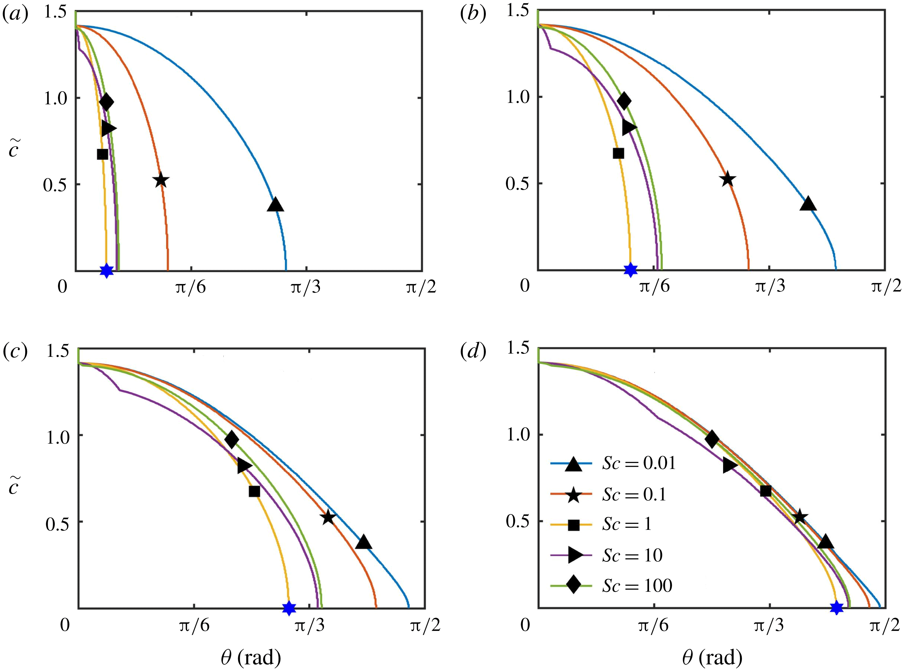
The neutral stability boundaries (3.13)–(3.15) on the
 $\unicode[STIX]{x1D703}$
–
 $\tilde{c}$
plane for (a)
 $F_{N}=-0.01$
, (b)
 $F_{N}=-0.1$
, (c)
 $F_{N}=-1$
, (d)
 $F_{N}=-10$
in an axisymmetric vortex. Within each plot, five different
 $Sc$
are considered, as indicated by the legend in (d). In each plot, the blue symbol on the
 $\unicode[STIX]{x1D703}$
-axis denotes the largest
 $\unicode[STIX]{x1D703}$
that is unstable in the fully inviscid analysis (3.6) for the corresponding value of
 $F_{N}$
. In each plot, the regions to the left and right of the neutral stability boundaries are unstable and stable, respectively.

Towards a physical interpretation of our results in figure 2, we write the neutral stability boundaries for a given
 $Sc$
in terms of (i)
 $F_{N}=F/N^{2}=(\dot{\unicode[STIX]{x1D713}}/r)(\ddot{\unicode[STIX]{x1D713}}+\dot{\unicode[STIX]{x1D713}}/r)/N^{2}$
, the ratio between the strength of the inviscid centrifugal instability and the stabilizing effect of stratification (square of the Froude number associated with the base flow), (ii)
 $\unicode[STIX]{x1D703}$
, the angle between the wave vector
 $\boldsymbol{k}$
and the out-of-plane
 $z$
-axis, and (iii)
 $\tilde{c}=c_{\unicode[STIX]{x1D708}}|\boldsymbol{k}|^{2}/\sqrt{-F}$
, a measure of the relative importance of the viscous effects in suppressing the inviscid, unstratified centrifugal instability (inverse of a Reynolds number-like parameter quantifying the ratio between viscous effects in the perturbations and the inertia in the base flow). We recall that
 $F<0$
, i.e.
 $F_{N}<0$
is the centrifugal instability criterion in the inviscid limit (3.6). In terms of these physically relevant parameters,
 $\unicode[STIX]{x1D6FC}_{1}$
and
 $\unicode[STIX]{x1D6FC}_{2}$
(3.9) can be written as
 $\unicode[STIX]{x1D6FC}_{1}=-2\cos ^{2}\unicode[STIX]{x1D703}/\tilde{c}^{2}$
and
 $\unicode[STIX]{x1D6FC}_{2}=-\!\sin ^{2}\unicode[STIX]{x1D703}/(F_{N}\tilde{c}^{2})$
, and the neutral stability boundary from (3.10) for
 $Sc\leqslant 1$
is
 $$\begin{eqnarray}1-{\displaystyle \frac{2\cos ^{2}\unicode[STIX]{x1D703}}{\tilde{c}^{2}}}-{\displaystyle \frac{Sc\sin ^{2}\unicode[STIX]{x1D703}}{F_{N}\tilde{c}^{2}}}=0,\end{eqnarray}$$
and those for
 $Sc>1$
from (3.11) to (3.12) become
 $$\begin{eqnarray}\displaystyle & \displaystyle 1-{\displaystyle \frac{2\cos ^{2}\unicode[STIX]{x1D703}}{\tilde{c}^{2}}}-{\displaystyle \frac{Sc\sin ^{2}\unicode[STIX]{x1D703}}{F_{N}\tilde{c}^{2}}}=0,\quad \text{for }\cos ^{2}\unicode[STIX]{x1D703}<{\displaystyle \frac{1+Sc}{Sc-1}}{\displaystyle \frac{\tilde{c}^{2}}{2}}, & \displaystyle\end{eqnarray}$$
 $$\begin{eqnarray}\displaystyle & \displaystyle {\displaystyle \frac{1}{Sc^{2}}}+{\displaystyle \frac{2}{Sc}}-{\displaystyle \frac{2\cos ^{2}\unicode[STIX]{x1D703}}{\tilde{c}^{2}}}-{\displaystyle \frac{\sin ^{2}\unicode[STIX]{x1D703}(1+Sc)}{2ScF_{N}\tilde{c}^{2}}}+1=0,\quad \text{for }\cos ^{2}\unicode[STIX]{x1D703}>{\displaystyle \frac{1+Sc}{Sc-1}}{\displaystyle \frac{\tilde{c}^{2}}{2}}.\qquad & \displaystyle\end{eqnarray}$$
We plot the stability boundaries in (3.13)–(3.15) on the
 $\unicode[STIX]{x1D703}$
–
 $\tilde{c}$
plane for various values of
 $Sc$
and
 $F_{N}$
in figure 3. Figure 3(a) corresponds to the strongly stratified case
 $F_{N}=-0.01$
, i.e. the stable stratification suppresses the inviscid instability for all
 $\unicode[STIX]{x1D703}>8.05^{\circ }$
(based on (3.6)). For
 $Sc=1$
the range of unstable
 $\unicode[STIX]{x1D703}$
for
 $\tilde{c}=0$
is
 $\unicode[STIX]{x1D703}\in [0,8.05^{\circ }]$
, and this range decreases as
 $\tilde{c}$
increases, before the instability is completely suppressed for
 $\tilde{c}>\sqrt{2}$
. For
 $Sc=0.1$
, the range of unstable
 $\unicode[STIX]{x1D703}$
(
 $\unicode[STIX]{x1D703}\in [0,21.4^{\circ }]$
) for
 $\tilde{c}\rightarrow 0$
is significantly larger when compared with the case of
 $Sc=1$
. The unstable
 $\unicode[STIX]{x1D703}$
range again decreases with
 $\tilde{c}$
before the entire range of
 $\unicode[STIX]{x1D703}\in [0,\unicode[STIX]{x03C0}/2]$
becomes stable for
 $\tilde{c}>\sqrt{2}$
. The neutral stability boundary for
 $Sc=0.01$
is qualitatively similar to that of
 $Sc=0.1$
, but with the unstable
 $\unicode[STIX]{x1D703}$
range for
 $\tilde{c}\rightarrow 0$
increasing to
 $\unicode[STIX]{x1D703}\in [0,54.74^{\circ }]$
. The neutral stability boundaries for
 $Sc=10$
,
 $100$
are in a close neighbourhood of that of
 $Sc=1$
, with the discontinuity in the slope of the neutral stability boundary being evident for
 $Sc=10$
. As pointed out earlier based on (3.12), the instability to the left of the discontinuity, i.e. for sufficiently small
 $\unicode[STIX]{x1D703}$
, is oscillatory in nature.
Figure 3(b–d) show the neutral stability boundaries for progressively weaker stratifications corresponding to
 $F_{N}=-0.1,-1$
and
 $-10$
, respectively. The range of unstable
 $\unicode[STIX]{x1D703}$
, in general, increases with the magnitude of
 $F_{N}$
. For
 $F_{N}=-0.1$
(figure 3
b), there are larger variations with
 $Sc$
for
 $Sc>1$
, when compared to the
 $F_{N}=-0.01$
case in figure 3(a). For
 $\tilde{c}\rightarrow 0$
, the range of unstable
 $\unicode[STIX]{x1D703}$
for
 $Sc=1$
increases with an increase in
 $|F_{N}|$
; for
 $Sc<1$
, this unstable range expands towards
 $\unicode[STIX]{x1D703}\in [0,\unicode[STIX]{x03C0}/2]$
as
 $Sc$
is decreased, and does so more rapidly with
 $Sc$
as
 $|F_{N}|$
is increased. For
 $Sc>1$
,
 $\tilde{c}\rightarrow 0$
, the range of unstable
 $\unicode[STIX]{x1D703}$
increases with
 $Sc$
, but saturates at some
 $\unicode[STIX]{x1D703}\in [0,\unicode[STIX]{x1D703}_{1}]$
for
 $Sc\gg 1$
;
 $\unicode[STIX]{x1D703}_{1}$
increases from approximately
 $11.31^{\circ }$
at
 $F_{N}=-0.01$
towards
 $\unicode[STIX]{x03C0}/2$
as
 $|F_{N}|$
is increased. Finally, for all
 $F_{N}$
, the region
 $\tilde{c}>\sqrt{2}$
is stable.
To analytically understand the trends in figure 3, we analyse the neutral stability boundaries in (3.13)–(3.15) in detail. For
 $Sc\leqslant 1$
, in the limit of
 $\tilde{c}\rightarrow 0$
, instability occurs for
 $\unicode[STIX]{x1D703}\in [0,\tan ^{-1}\sqrt{-2F_{N}/Sc}]$
, the boundary of which is indicated by the blue stars in figure 3 for
 $Sc=1$
. For
 $Sc\ll 1$
, and
 $\tilde{c}\rightarrow 0$
, the entire range of
 $\unicode[STIX]{x1D703}\in [0,\unicode[STIX]{x03C0}/2]$
is therefore unstable. Consequently, in the limit of
 $\tilde{c}\rightarrow 0$
, even if
 $|F_{N}|$
is so small that only an infinitesimally small range around
 $\unicode[STIX]{x1D703}=0$
is unstable for
 $Sc=1$
, a sufficiently small
 $Sc$
will always render the entire range of
 $\unicode[STIX]{x1D703}\in [0,\unicode[STIX]{x03C0}/2]$
unstable. For
 $Sc>1$
, and
 $\tilde{c}\rightarrow 0$
, the range of unstable
 $\unicode[STIX]{x1D703}$
is
 $\unicode[STIX]{x1D703}\in [0,\tan ^{-1}\sqrt{-4ScF_{N}/(1+Sc)}]$
; for
 $Sc\gg 1$
, the unstable
 $\unicode[STIX]{x1D703}$
range expands to
 $\unicode[STIX]{x1D703}\in [0,\unicode[STIX]{x1D703}_{1}]$
, where
 $\unicode[STIX]{x1D703}_{1}=\tan ^{-1}\sqrt{-4F_{N}}$
. In summary, for
 $\tilde{c}\rightarrow 0$
, the upper limit of the unstable range in
 $\unicode[STIX]{x1D703}$
moves from
 $\tan ^{-1}\sqrt{-2F_{N}}$
to
 $\tan ^{-1}\sqrt{-4F_{N}}$
as
 $Sc$
is increased from
 $Sc=1$
to
 $Sc\rightarrow \infty$
. Finally, for
 $\unicode[STIX]{x1D703}=0$
, the corresponding
 $\tilde{c}$
on the neutral stability boundary is always given by (3.13) or (3.14), irrespective of the value of
 $Sc$
, owing to which the region
 $\tilde{c}>\sqrt{2}$
is stable for all
 $Sc$
and
 $F_{N}$
. As a concluding point, we note that the entire analysis for axisymmetric vortices is trivially extended to the case with background rotation
 $\unicode[STIX]{x1D6FA}_{z}$
by replacing
 $\unicode[STIX]{x1D713}$
with
 $\unicode[STIX]{x1D713}+\unicode[STIX]{x1D6FA}_{z}r^{2}/2$
.
4 Results – elliptical vortex
In this section, we investigate the effects of
 $Sc$
on the instabilities in an elliptical vortex described by the streamfunction (Landman & Saffman Reference Landman and Saffman1987):
 $$\begin{eqnarray}\unicode[STIX]{x1D713}=-{\displaystyle \frac{\unicode[STIX]{x1D6FE}}{2}}(y^{2}+x^{2})-{\displaystyle \frac{\unicode[STIX]{x1D716}}{2}}(y^{2}-x^{2}),\end{eqnarray}$$
where
 $\boldsymbol{u}_{B}=(-\unicode[STIX]{x2202}\unicode[STIX]{x1D713}/\unicode[STIX]{x2202}y)\hat{\boldsymbol{e}}_{x}+(\unicode[STIX]{x2202}\unicode[STIX]{x1D713}/\unicode[STIX]{x2202}x)\hat{\boldsymbol{e}}_{y}$
. The stable density stratification
 $\unicode[STIX]{x1D70C}_{B}(z)$
is characterized by the corresponding buoyancy frequency
 $N=\sqrt{(-g/\unicode[STIX]{x1D70C}_{o})\,\text{d}\unicode[STIX]{x1D70C}_{B}/\text{d}z}$
, with gravity being given by
 $\boldsymbol{g}=-g\hat{\boldsymbol{e}}_{z}$
. The base flow described by (4.1) corresponds to a uniform vorticity of
 $2\unicode[STIX]{x1D6FE}$
everywhere, and the ellipticity parameter
 $\unicode[STIX]{x1D716}$
 $(0\leqslant \unicode[STIX]{x1D716}<\unicode[STIX]{x1D6FE})$
quantifies the eccentricity of the streamlines, which are circular for
 $\unicode[STIX]{x1D716}=0$
.
Any fluid particle goes around the elliptical streamlines exactly once in a time period
 $T=2\unicode[STIX]{x03C0}/\unicode[STIX]{x1D714}$
, with
 $\unicode[STIX]{x1D714}=\sqrt{\unicode[STIX]{x1D6FE}^{2}-\unicode[STIX]{x1D716}^{2}}$
. As shown by Landman & Saffman (Reference Landman and Saffman1987), the solution to the wave vector equation (2.9) for the base flow in (4.1) is given by
 $$\begin{eqnarray}\boldsymbol{k}=[k_{x},k_{y},k_{z}]=k_{o}[-\!\sin \unicode[STIX]{x1D703}\cos \unicode[STIX]{x1D714}(t-t_{o}),\unicode[STIX]{x1D6FC}\sin \unicode[STIX]{x1D703}\sin \unicode[STIX]{x1D714}(t-t_{o}),\cos \unicode[STIX]{x1D703}],\end{eqnarray}$$
where
 $\unicode[STIX]{x1D6FC}=\sqrt{(\unicode[STIX]{x1D6FE}+\unicode[STIX]{x1D716})/(\unicode[STIX]{x1D6FE}-\unicode[STIX]{x1D716})}$
,
 $k_{o}$
is the wave vector magnitude at
 $t=t_{o}$
, and
 $\unicode[STIX]{x1D703}$
is the angle made by
 $\boldsymbol{k}$
with the
 $z$
-axis at
 $t=t_{o}$
. All the wave vectors are therefore periodic with the same period as that of the streamlines, and hence Floquet theory is applicable to study the growth or decay of perturbations governed by the local stability equations (2.12)–(2.13). Furthermore, for a given streamline, it suffices to consider
 $t_{o}=0$
, which is the case we study in the rest of this paper. A straightforward extension of the study by Landman & Saffman (Reference Landman and Saffman1987) leads to
 $\unicode[STIX]{x1D70E}=\unicode[STIX]{x1D70E}_{o}-(\unicode[STIX]{x1D714}/2\unicode[STIX]{x03C0})c_{\unicode[STIX]{x1D708}}\int _{0}^{2\unicode[STIX]{x03C0}/\unicode[STIX]{x1D714}}|\boldsymbol{k}|^{2}\,\text{d}t$
, where
 $\unicode[STIX]{x1D70E}$
is the growth rate for
 $\unicode[STIX]{x1D708}=\unicode[STIX]{x1D705}$
, i.e.
 $Sc=1$
, and
 $\unicode[STIX]{x1D70E}_{o}$
the inviscid (
 $\unicode[STIX]{x1D708}=\unicode[STIX]{x1D705}=0$
) growth rate. For the time-dependent wave vector given in (4.2), the relation between the viscous growth rate for
 $Sc=1$
and the inviscid growth rate reduces to
 $\unicode[STIX]{x1D70E}=\unicode[STIX]{x1D70E}_{o}-c_{\unicode[STIX]{x1D708}}k_{o}^{2}(1+((\unicode[STIX]{x1D6FC}^{2}-1)/2)\sin ^{2}\unicode[STIX]{x1D703})$
.
Making use of the following transformation (Landman & Saffman Reference Landman and Saffman1987):
 $$\begin{eqnarray}\left\{\begin{array}{@{}c@{}}\hat{\boldsymbol{a}}\\ \hat{b}\end{array}\right\}=\left\{\begin{array}{@{}c@{}}\boldsymbol{a}\\ b\end{array}\right\}\exp \left(c_{\unicode[STIX]{x1D708}}\int _{0}^{t}|\boldsymbol{k}|^{2}\,\text{d}\unicode[STIX]{x1D70F}\right),\end{eqnarray}$$
and defining
 $\tilde{t}=\unicode[STIX]{x1D6FE}t$
,
 $\tilde{b}=\hat{b}/\unicode[STIX]{x1D6FE}$
, equations (2.12)–(2.13) reduce to
 $$\begin{eqnarray}\displaystyle {\displaystyle \frac{\text{d}\hat{\boldsymbol{a}}}{\text{d}\tilde{t}}} & = & \displaystyle (1+\tilde{\unicode[STIX]{x1D716}})\hat{a}_{y}\hat{\boldsymbol{e}}_{x}-(1-\tilde{\unicode[STIX]{x1D716}})\hat{a}_{x}\hat{\boldsymbol{e}}_{y}+{\displaystyle \frac{\boldsymbol{k}}{k_{o}}}{\displaystyle \frac{[(1+\tilde{\unicode[STIX]{x1D716}})\hat{a}_{y}\sin \unicode[STIX]{x1D703}\cos \tilde{\unicode[STIX]{x1D714}}\tilde{t}+\unicode[STIX]{x1D6FC}(1-\tilde{\unicode[STIX]{x1D716}})\hat{a}_{x}\sin \unicode[STIX]{x1D703}\sin \tilde{\unicode[STIX]{x1D714}}\tilde{t}]}{(1+(\unicode[STIX]{x1D6FC}^{2}-1)\sin ^{2}\unicode[STIX]{x1D703}\sin ^{2}\tilde{\unicode[STIX]{x1D714}}\tilde{t})}}\nonumber\\ \displaystyle & & \displaystyle -\,\tilde{b}\left[\hat{\boldsymbol{e}}_{z}-{\displaystyle \frac{\boldsymbol{k}}{k_{o}}}{\displaystyle \frac{\cos \unicode[STIX]{x1D703}}{(1+(\unicode[STIX]{x1D6FC}^{2}-1)\sin ^{2}\unicode[STIX]{x1D703}\sin ^{2}\tilde{\unicode[STIX]{x1D714}}\tilde{t})}}\right]\!,\end{eqnarray}$$
 $$\begin{eqnarray}{\displaystyle \frac{\text{d}\tilde{b}}{\text{d}\tilde{t}}}=\widetilde{N}^{2}\hat{a}_{z}+E_{\unicode[STIX]{x1D6FE}}\left(1-{\displaystyle \frac{1}{Sc}}\right)[1+(\unicode[STIX]{x1D6FC}^{2}-1)\sin ^{2}\unicode[STIX]{x1D703}\sin ^{2}\tilde{\unicode[STIX]{x1D714}}\tilde{t}]\tilde{b},\end{eqnarray}$$
where
 $$\begin{eqnarray}\left.\begin{array}{@{}c@{}}\tilde{\unicode[STIX]{x1D716}}=\unicode[STIX]{x1D716}/\unicode[STIX]{x1D6FE},\\ \widetilde{N}=N/\unicode[STIX]{x1D6FE},\\ E_{\unicode[STIX]{x1D6FE}}=c_{\unicode[STIX]{x1D708}}k_{o}^{2}/\unicode[STIX]{x1D6FE}.\end{array}\right\}\end{eqnarray}$$
The parameters
 $\unicode[STIX]{x1D6FC}$
and
 $\tilde{\unicode[STIX]{x1D714}}$
are now written as
 $\unicode[STIX]{x1D6FC}=\sqrt{(1+\tilde{\unicode[STIX]{x1D716}})/(1-\tilde{\unicode[STIX]{x1D716}})}$
and
 $\tilde{\unicode[STIX]{x1D714}}=\sqrt{1-\tilde{\unicode[STIX]{x1D716}}^{2}}$
. In summary, the governing non-dimensional parameters are (i)
 $\tilde{\unicode[STIX]{x1D716}}$
, the relative strength of eccentricity with respect to the vorticity, (ii)
 $\widetilde{N}$
, the relative strength of stable stratification with respect to the vorticity, (iii)
 $E_{\unicode[STIX]{x1D6FE}}$
, the relative strength of viscous effects with respect to the vorticity of the base flow, (iv)
 $\unicode[STIX]{x1D703}$
, the initial angle between the wave vector and the
 $z$
-axis, and (v)
 $Sc$
, the Schmidt number. The scaled growth rate
 $\unicode[STIX]{x1D70E}^{\unicode[STIX]{x1D6FE}}=\unicode[STIX]{x1D70E}/\unicode[STIX]{x1D6FE}$
is determined entirely in terms of these five non-dimensional parameters.
It is noteworthy that (4.4) and (4.5) coincide with the inviscid local stability equations but for the additional last term in (4.5). In other words, in the limit of either
 $E_{\unicode[STIX]{x1D6FE}}=0$
or
 $Sc=1$
, the growth rates for (4.4) and (4.5) reduce to the inviscid growth rates. The overall growth rate
 $\unicode[STIX]{x1D70E}$
(in time
 $t$
) for (2.12) and (2.13) can now be decomposed as
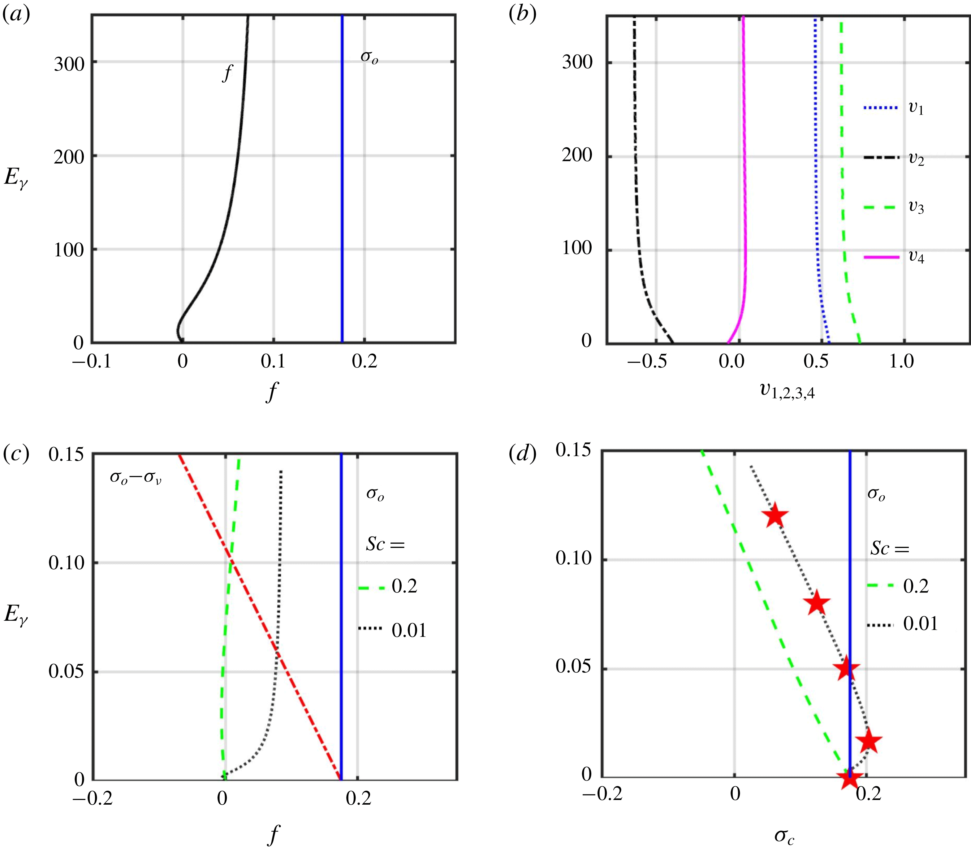
 $$\begin{eqnarray}{\displaystyle \frac{\unicode[STIX]{x1D70E}}{\unicode[STIX]{x1D6FE}}}=\unicode[STIX]{x1D70E}_{o}(\tilde{\unicode[STIX]{x1D716}},\widetilde{N},\unicode[STIX]{x1D703})+f(\tilde{\unicode[STIX]{x1D716}},\widetilde{N},\unicode[STIX]{x1D703},E_{\unicode[STIX]{x1D6FE}}^{Sc})-E_{\unicode[STIX]{x1D6FE}}\left(1+{\displaystyle \frac{(\unicode[STIX]{x1D6FC}^{2}-1)}{2}}\sin ^{2}\unicode[STIX]{x1D703}\right)\!,\end{eqnarray}$$
where
 $E_{\unicode[STIX]{x1D6FE}}^{Sc}=E_{\unicode[STIX]{x1D6FE}}(1-1/Sc)$
is the parameter appearing in the last term in (4.5). The function
 $f$
represents the
 $Sc$
-correction to be added to the inviscid growth rate
 $\unicode[STIX]{x1D70E}_{o}$
to obtain the growth rate for the (4.4) and (4.5). The viscous suppression given by the last term in the right-hand side of (4.7) is then added to
 $\unicode[STIX]{x1D70E}_{o}+f$
to construct the overall growth rate
 $\unicode[STIX]{x1D70E}$
. For a given
 $(\tilde{\unicode[STIX]{x1D716}},\widetilde{N},\unicode[STIX]{x1D703})$
, the
 $Sc$
-dependence is present only in
 $f$
through the parameter
 $E_{\unicode[STIX]{x1D6FE}}^{Sc}$
, and hence makes it possible to construct
 $\unicode[STIX]{x1D70E}$
versus
 $E_{\unicode[STIX]{x1D6FE}}$
at various
 $Sc$
based on
 $\unicode[STIX]{x1D70E}$
versus
 $E_{\unicode[STIX]{x1D6FE}}$
at one given
 $Sc\neq 1$
. In the rest of this section, we refer to
 $\unicode[STIX]{x1D70E}^{\unicode[STIX]{x1D6FE}}=\unicode[STIX]{x1D70E}/\unicode[STIX]{x1D6FE}$
as the growth rate, and we skip the superscript
 $\unicode[STIX]{x1D6FE}$
for convenience.
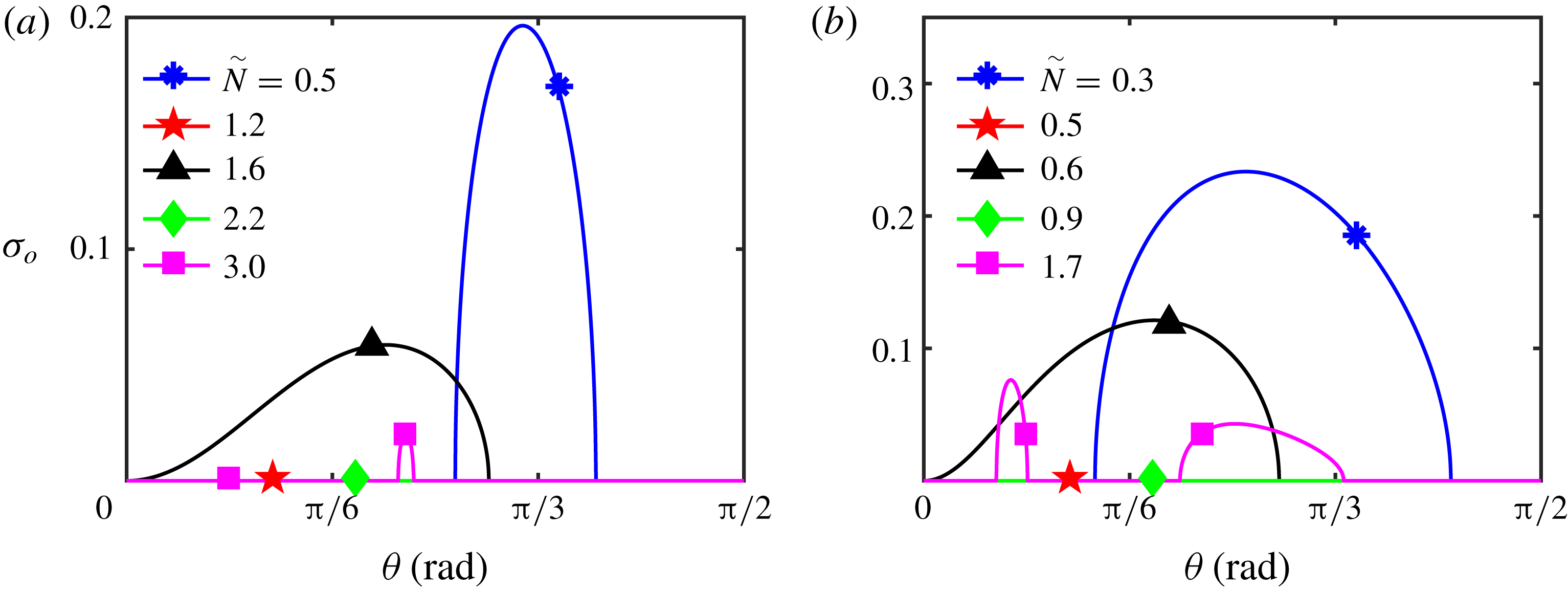
Inviscid (
 $\unicode[STIX]{x1D708}=\unicode[STIX]{x1D705}=0$
) growth rate
 $\unicode[STIX]{x1D70E}_{o}$
plotted as a function of
 $\unicode[STIX]{x1D703}$
for the elliptical vortex with (a)
 $\tilde{\unicode[STIX]{x1D716}}=0.5$
, (b)
 $\tilde{\unicode[STIX]{x1D716}}=0.9$
. Within each plot, five different values of
 $\widetilde{N}$
, as indicated in the respective legends, are considered.

We start by presenting the inviscid (
 $\unicode[STIX]{x1D708}=\unicode[STIX]{x1D705}=0$
) stability characteristics of the elliptical vortex for various values of
 $\tilde{\unicode[STIX]{x1D716}}$
,
 $\widetilde{N}$
and
 $\unicode[STIX]{x1D703}$
. We recall that inviscid analyses of the elliptical vortex without and with out-of-plane stratification have previously been reported by Bayly (Reference Bayly1986) and Miyazaki & Fukumoto (Reference Miyazaki and Fukumoto1992), respectively. Figure 4(a) shows the inviscid growth rate
 $\unicode[STIX]{x1D70E}_{o}$
as a function of
 $\unicode[STIX]{x1D703}$
for various values of
 $\widetilde{N}$
and a fixed
 $\tilde{\unicode[STIX]{x1D716}}=0.5$
. For the unstratified case of
 $\widetilde{N}=0$
, we recover the well-known elliptic instability (Kerswell Reference Kerswell2002) that occurs in a finite-width neighbourhood (
 $0.74<\unicode[STIX]{x1D703}<1.12$
rad) around
 $\unicode[STIX]{x1D703}=\unicode[STIX]{x03C0}/3$
with a corresponding maximum growth rate of
 $\unicode[STIX]{x1D70E}=0.26$
. Upon increasing
 $\widetilde{N}$
to
 $\widetilde{N}=0.5$
, the maximum growth rate decreases in magnitude, and the range of unstable
 $\unicode[STIX]{x1D703}$
moves to the right to
 $0.83<\unicode[STIX]{x1D703}<1.19$
rad (figure 4
a). The elliptic instability is completely absent at
 $\widetilde{N}=1.2$
. Upon closer investigation, we find that the elliptic instability that is present at
 $\widetilde{N}=0$
gets completely suppressed at
 $\widetilde{N}=0.9$
for
 $\tilde{\unicode[STIX]{x1D716}}=0.5$
.
A further increase in
 $\widetilde{N}$
to
 $\widetilde{N}=1.6$
shows the appearance of a new instability in the range
 $0<\unicode[STIX]{x1D703}<0.92$
rad. This new instability is absent at
 $\widetilde{N}=2.2$
, and yet another new instability is seen at
 $\widetilde{N}=3$
. In summary, for
 $\tilde{\unicode[STIX]{x1D716}}=0.5$
, as
 $\widetilde{N}$
is increased from zero, the original elliptic instability present at
 $\widetilde{N}=0$
first gets suppressed, followed by the appearance of a new instability, which is also suppressed at a larger
 $\widetilde{N}$
. Finally, at sufficiently large
 $\widetilde{N}$
, there emerges yet another new instability. All the observations in figure 4(a) are consistent with the results of Miyazaki & Fukumoto (Reference Miyazaki and Fukumoto1992). A similar sequence of suppression and emergence of instabilities occurs as
 $\widetilde{N}$
is increased from zero for
 $\tilde{\unicode[STIX]{x1D716}}=0.9$
(figure 4
b), but over a smaller range of
 $\widetilde{N}$
than for
 $\tilde{\unicode[STIX]{x1D716}}=0.5$
. Interestingly, at
 $\tilde{\unicode[STIX]{x1D716}}=0.9$
, the second new instability that occurs at large
 $\widetilde{N}$
contains two separate peaks when
 $\unicode[STIX]{x1D70E}$
is plotted as a function of
 $\unicode[STIX]{x1D703}$
, occurring specifically at
 $\unicode[STIX]{x1D703}=0.22$
rad and
 $\unicode[STIX]{x1D703}=0.78$
rad for
 $\widetilde{N}=1.7$
in figure 4(b).
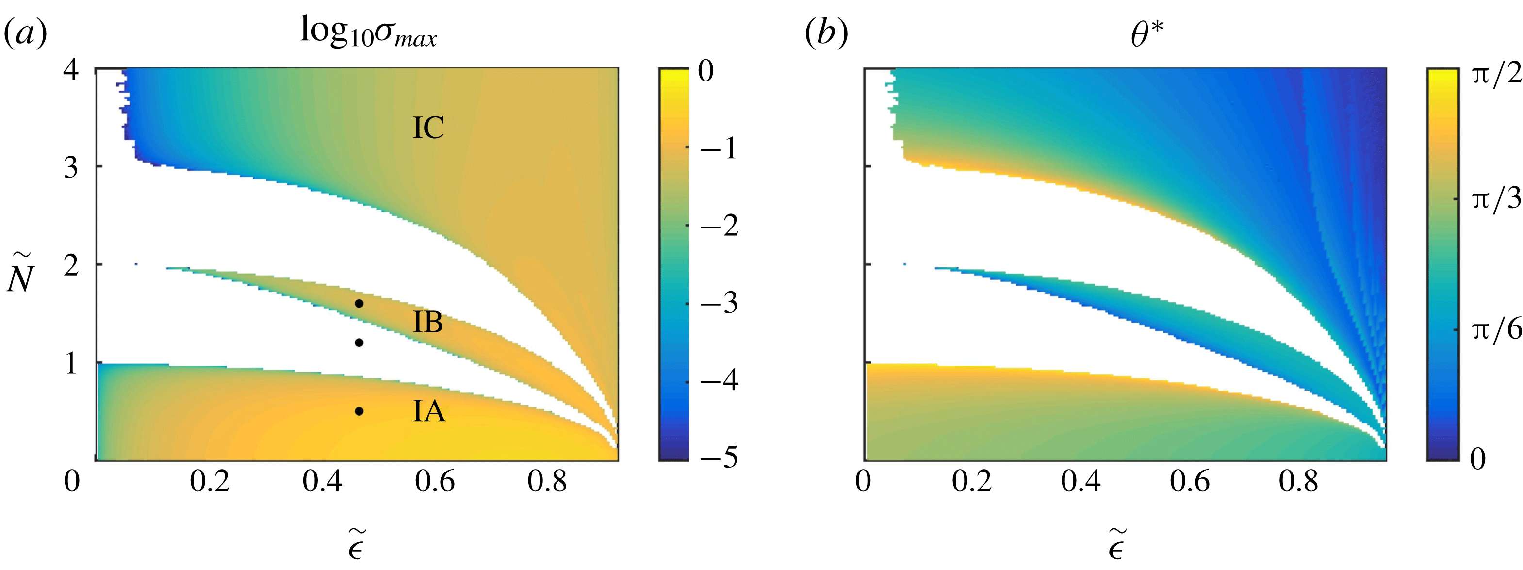
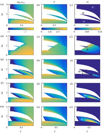
Inviscid instabilities on the
 $\tilde{\unicode[STIX]{x1D716}}$
–
 $\widetilde{N}$
plane for the elliptical vortex. (a) The maximum growth rate
 $\unicode[STIX]{x1D70E}_{max}$
(maximum
 $\unicode[STIX]{x1D70E}$
over
 $0\leqslant \unicode[STIX]{x1D703}\leqslant \unicode[STIX]{x03C0}/2$
), and (b) the corresponding location
 $\unicode[STIX]{x1D703}^{\ast }$
where
 $\unicode[STIX]{x1D70E}_{max}$
occurs, plotted as a function of
 $\tilde{\unicode[STIX]{x1D716}}$
and
 $\widetilde{N}$
in the inviscid limit of
 $c_{\unicode[STIX]{x1D708}}=c_{\unicode[STIX]{x1D705}}=0$
. The stable regions are shown in white in both (a) and (b). The black points in (a) denote parameter values considered in figure 6. Instability regions IB and IC extend all the way to
 $\tilde{\unicode[STIX]{x1D716}}=0$
, though the corresponding small
 $\tilde{\unicode[STIX]{x1D716}}({\lesssim}0.1)$
regions are not accurately depicted as unstable owing to the numerical issues discussed at the end of § 2.

In figure 5, we show the continuous variation of the dominant inviscid (
 $c_{\unicode[STIX]{x1D708}}=c_{\unicode[STIX]{x1D705}}=0$
) instability characteristics of the elliptical vortex, with
 $\tilde{\unicode[STIX]{x1D716}}$
and
 $\widetilde{N}$
. In figure 5(a), we plot the maximum
 $\unicode[STIX]{x1D70E}_{o}$
(maximized over
 $0\leqslant \unicode[STIX]{x1D703}\leqslant \unicode[STIX]{x03C0}/2$
, denoted by
 $\unicode[STIX]{x1D70E}_{max}$
) as a function of
 $\tilde{\unicode[STIX]{x1D716}}$
and
 $\widetilde{N}$
; the corresponding angle
 $\unicode[STIX]{x1D703}^{\ast }$
associated with the most unstable wave vector is plotted in figure 5(b). For small
 $\tilde{\unicode[STIX]{x1D716}}$
, as reported in figure 4(a) for
 $\tilde{\unicode[STIX]{x1D716}}=0.5$
, the elliptic instability (henceforth referred to as instability IA) gets suppressed at
 $\widetilde{N}\approx 1$
. The value of
 $\unicode[STIX]{x1D703}^{\ast }$
corresponding to instability IA is close to
 $\unicode[STIX]{x03C0}/3$
for
 $\widetilde{N}=0$
, then increases towards
 $\unicode[STIX]{x1D703}^{\ast }=\unicode[STIX]{x03C0}/2$
as
 $\widetilde{N}$
is increased. The threshold
 $\widetilde{N}=\widetilde{N}_{t}$
, above which instability IA disappears, decreases with increasing
 $\tilde{\unicode[STIX]{x1D716}}$
. At all
 $\tilde{\unicode[STIX]{x1D716}}$
, an increase in
 $\widetilde{N}$
beyond the corresponding
 $\widetilde{N}_{t}$
results in the birth of a new instability branch (henceforth referred to as instability IB), which again gets suppressed at even larger
 $\widetilde{N}$
. The values of
 $\widetilde{N}$
at which instability IB is born and subsequently suppressed also decrease with increasing
 $\tilde{\unicode[STIX]{x1D716}}$
. The range of
 $\widetilde{N}$
over which instability IB occurs is the largest for an intermediate value of
 $\tilde{\unicode[STIX]{x1D716}}\approx 0.75$
; the corresponding
 $\unicode[STIX]{x1D703}^{\ast }$
associated with instability IB is noticeably smaller than
 $\unicode[STIX]{x03C0}/3$
, taking values in and around
 $\unicode[STIX]{x03C0}/6$
. With further increase in
 $\widetilde{N}$
after instability IB is suppressed, we observe the birth of yet another instability branch (henceforth referred to as instability IC) for all
 $\tilde{\unicode[STIX]{x1D716}}$
, and it remains unsuppressed at least until
 $\widetilde{N}=4$
. The most unstable wave vector associated with instability IC corresponds to relatively small values of
 $\unicode[STIX]{x1D703}^{\ast }$
, and it approaches zero as
 $\tilde{\unicode[STIX]{x1D716}}$
and
 $\widetilde{N}$
are increased. The instabilities IA, IB and IC are described in Miyazaki & Fukumoto (Reference Miyazaki and Fukumoto1992) as the subharmonic, fundamental and superharmonic instabilities, respectively, owing to their relation with parametric resonance phenomenon associated with inertial gravity waves. To study the effects of Schmidt number, the diffusion terms in the local stability equations are switched on, and different values of
 $\widetilde{N}$
at a fixed
 $\tilde{\unicode[STIX]{x1D716}}=0.5$
, as indicated by the black dots in figure 5(a), are considered. These points are chosen so as to investigate the effects of
 $Sc$
on both the inviscidly unstable and stable regimes.
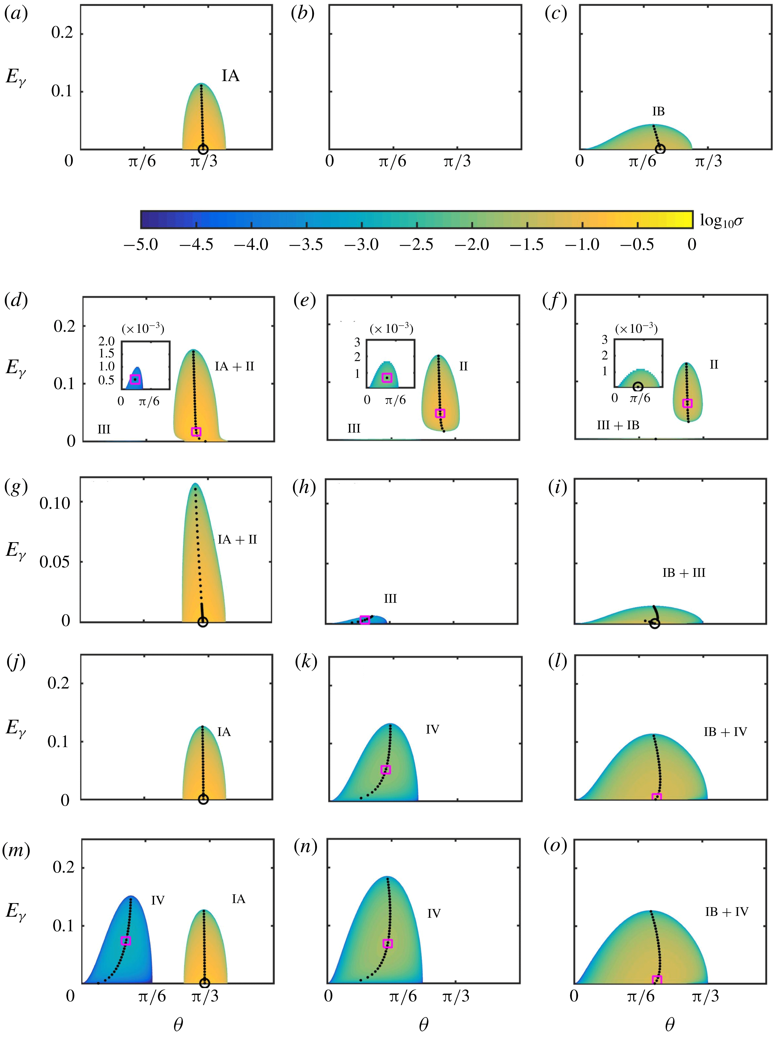
Growth rate
 $\unicode[STIX]{x1D70E}$
on the
 $\unicode[STIX]{x1D703}$
–
 $E_{\unicode[STIX]{x1D6FE}}$
plane for various (
 $\widetilde{N},Sc$
) combinations, all at
 $\tilde{\unicode[STIX]{x1D716}}=0.5$
. The stable regions are shown in white. The columns (left to right) correspond to
 $\widetilde{N}=0.5,1.2,1.6$
(also shown as black dots in figure 5
a). The rows (top to bottom) correspond to
 $Sc=1,0.01,0.2,10,100$
. The black dotted lines in each plot track the most unstable
 $\unicode[STIX]{x1D703}$
as
 $E_{\unicode[STIX]{x1D6FE}}$
is varied within each instability region. The circles/triangles in each plot denote the location of maximum
 $\unicode[STIX]{x1D70E}$
within the corresponding instability region (black circle if
 $E_{\unicode[STIX]{x1D6FE}}=0$
and magenta triangle if
 $E_{\unicode[STIX]{x1D6FE}}>0$
at the locations). Insets in (d–f) show a zoomed-in view of small instability regions that lie close to the
 $E_{\unicode[STIX]{x1D6FE}}=0$
axis. The instability types present within the unstable regions are indicated in each plot.

Figure 6 shows the effects of
 $Sc$
for
 $\tilde{\unicode[STIX]{x1D716}}=0.5$
, and
 $\widetilde{N}=0.5$
(left column),
 $1.2$
(middle column) and
 $1.6$
(right column). As shown by the black dots in figure 5(a), these values of
 $\widetilde{N}$
are in the inviscidly unstable (IA), stable and unstable (IB) regions, respectively, for
 $\tilde{\unicode[STIX]{x1D716}}=0.5$
. The rows in figure 6 correspond to
 $Sc=1,0.01,0.2,10,100$
. We recall from earlier in this section that at
 $Sc=1$
, viscous effects serve only to suppress the inviscid instabilities. In each plot in figure 6, we plot
 $\log _{10}\unicode[STIX]{x1D70E}$
as a function of
 $\unicode[STIX]{x1D703}$
on the
 $x$
-axis and
 $E_{\unicode[STIX]{x1D6FE}}$
on the
 $y$
-axis for the corresponding values of
 $(\tilde{\unicode[STIX]{x1D716}},\widetilde{N},Sc)$
.
As shown in figure 6(a), for
 $(\tilde{\unicode[STIX]{x1D716}},\widetilde{N},Sc)=(0.5,0.5,1)$
, an increase in
 $E_{\unicode[STIX]{x1D6FE}}$
results in a decrease in
 $\unicode[STIX]{x1D70E}$
for a given
 $\unicode[STIX]{x1D703}\in [0.83,1.19]$
rad. At
 $E_{\unicode[STIX]{x1D6FE}}\approx 0.115$
, the inviscid instability IA that is present at
 $E_{\unicode[STIX]{x1D6FE}}=0$
for all
 $\unicode[STIX]{x1D703}\in [0.83,1.19]$
rad is completely suppressed by viscous effects. For a given
 $E_{\unicode[STIX]{x1D6FE}}\leqslant 0.115$
, the most unstable
 $\unicode[STIX]{x1D703}$
occurs at
 $\unicode[STIX]{x1D703}\approx \unicode[STIX]{x03C0}/3$
, as indicated by the nearly vertical black dotted line. As expected for
 $Sc=1$
, the overall maximum growth rate occurs on the
 $E_{\unicode[STIX]{x1D6FE}}=0$
axis. In the limit of
 $E_{\unicode[STIX]{x1D6FE}}=0$
,
 $\unicode[STIX]{x1D70E}$
is independent of
 $Sc$
, as both viscous and density diffusion effects are absent. However, the value of
 $E_{\unicode[STIX]{x1D6FE}}$
below which
 $\unicode[STIX]{x1D70E}$
is almost identical to that in the inviscid limit of
 $E_{\unicode[STIX]{x1D6FE}}=0$
depends on the specific value of
 $Sc$
.
For
 $Sc=0.01$
(figure 6
d), as we increase
 $E_{\unicode[STIX]{x1D6FE}}$
from zero, the location of the most unstable
 $\unicode[STIX]{x1D703}$
(indicated by the black dotted line) moves slightly to the left, which is in contrast with the case of
 $Sc=1$
(figure 6
a). Strikingly, the threshold value of
 $E_{\unicode[STIX]{x1D6FE}}$
above which no instability occurs at all
 $\unicode[STIX]{x1D703}$
is larger for
 $Sc=0.01$
than that for
 $Sc=1$
. The maximum
 $\unicode[STIX]{x1D70E}$
on the entire
 $\unicode[STIX]{x1D703}$
–
 $E_{\unicode[STIX]{x1D6FE}}$
plane occurs at
 $(0.93,0.017)$
for
 $Sc=0.01$
(indicated by the magenta triangle in figure 6
d), while it occurs at
 $(1.105,0)$
for
 $Sc=1$
(indicated by the black circle in figure 6
a). The occurrence of maximum
 $\unicode[STIX]{x1D70E}$
at a non-zero value of
 $E_{\unicode[STIX]{x1D6FE}}$
can manifest only as a result of
 $Sc\neq 1$
, as viscous effects are purely suppressive for
 $Sc=1$
; this is suggestive of either a new branch of instability or a modification of the inviscid instabilities which are known to exist for
 $Sc=1$
. In either case, we attribute the
 $Sc\neq 1$
effect in the region of instability IA in figure 6(d) to an instability II; a detailed discussion on whether instability II is connected to the inviscid instabilities or represents a completely new instability that is not present for
 $Sc=1$
is presented in (§ 4.1). In summary, the instability region in
 $\unicode[STIX]{x1D703}\in [0.80,1.19]$
rad in figure 6(d) seems to comprise instability II present along with the original inviscid instability IA at
 $Sc=0.01$
. Additionally, we observe an instability region at small
 $E_{\unicode[STIX]{x1D6FE}}$
for
 $\unicode[STIX]{x1D703}\in [0,0.5]$
rad (see inset of figure 6
d), which is not present for
 $Sc=1$
(figure 6
a). Furthermore, the maximum
 $\unicode[STIX]{x1D70E}$
within this instability region occurs at a finite
 $E_{\unicode[STIX]{x1D6FE}}$
, which is clearly a
 $Sc\neq 1$
effect. Interestingly, the imaginary part of the complex growth rate is non-zero throughout this small instability region shown in the inset of figure 6(d), thus suggesting that it is distinct from the inviscid instabilities, whose complex growth rates are purely real. Henceforth, we denote the instability in this region as instability III, and is discussed in further detail in § 4.2. For
 $Sc=0.2$
(figure 6
g), we again observe the occurrence of instability II, as suggested by the small but noticeable shift of the black dotted line (that tracks the most unstable
 $\unicode[STIX]{x1D703}$
as
 $E_{\unicode[STIX]{x1D6FE}}$
is varied) towards smaller
 $\unicode[STIX]{x1D703}$
values as
 $E_{\unicode[STIX]{x1D6FE}}$
is increased. The overall maximum growth rate, however, occurs on the
 $E_{\unicode[STIX]{x1D6FE}}=0$
axis (black circle in figure 6
g) similar to the inviscid instability IA.
For
 $Sc=10$
(figure 6
j), the variation of
 $\unicode[STIX]{x1D70E}$
on the
 $\unicode[STIX]{x1D703}$
–
 $E_{\unicode[STIX]{x1D6FE}}$
plane is almost identical to that of
 $Sc=1$
(figure 6
a). At
 $Sc=100$
(figure 6
m), apart from instability IA, which seems minimally affected by
 $Sc>1$
, a new instability region (henceforth referred to as instability IV) occurring at relatively smaller values of
 $\unicode[STIX]{x1D703}$
is seen. The maximum growth rate associated with instability IV occurs at
 $(\unicode[STIX]{x1D703},E_{\unicode[STIX]{x1D6FE}})$
=
 $(0.36,0.07)$
, though being weaker than the dominant instability IA. The connection, or lack thereof, of instability IV with the inviscid instabilities is discussed in (§ 4.3). In summary, for
 $(\tilde{\unicode[STIX]{x1D716}},\widetilde{N})=(0.5,0.5)$
, inviscid instability IA is present for all
 $Sc$
in the range
 $0.01\leqslant Sc\leqslant 100$
, being quantitatively more strongly affected by
 $Sc<1$
than by
 $Sc>1$
. Furthermore, seemingly new instabilities II and III emerge for
 $Sc<1$
, and are characterized by their most unstable
 $E_{\unicode[STIX]{x1D6FE}}$
occurring at finite values. For sufficiently large
 $Sc>1$
, we find yet another seemingly new instability IV, which is characterized by its occurrence at relatively small
 $\unicode[STIX]{x1D703}$
and the maximum growth rate at finite
 $E_{\unicode[STIX]{x1D6FE}}$
.
In figure 6(b,e,h,k,n), we consider
 $\tilde{\unicode[STIX]{x1D716}}=0.5$
again, but with a stronger stratification than in panels (a,d,g,j,m). Specifically, the chosen value
 $\widetilde{N}=1.2$
is such that the inviscid instability IA has been suppressed by stratification effects, as is evident from figure 5(a). As a result, there are no instabilities for
 $Sc=1$
(figure 6
b). For
 $Sc=0.01$
(figure 6
e), we now observe instability II present in isolation, resulting in an instability region that is disconnected from the
 $E_{\unicode[STIX]{x1D6FE}}=0$
axis. The maximum
 $\unicode[STIX]{x1D70E}$
for instability II at
 $Sc=0.01$
occurs at
 $(\unicode[STIX]{x1D703}^{\ast },E_{\unicode[STIX]{x1D6FE}}^{\ast })=(0.924,0.046)$
. Also present in figure 6(e) is an instability III region very close to the
 $E_{\unicode[STIX]{x1D6FE}}=0$
axis occurring at approximately
 $\unicode[STIX]{x1D703}=0.5$
. The inset in figure 6(e) shows a magnified plot of the instability III region, where we clearly observe the most unstable
 $E_{\unicode[STIX]{x1D6FE}}$
to be finite. Additionally, the instability III region, as observed in figure 6(d), is again characterized by a non-zero imaginary part for the complex growth rate and is hence oscillatory in nature. At
 $Sc=0.2$
(figure 6
h), while instability II is absent, the presence of instability III is more evident, with the maximum growth rate occurring at
 $(\unicode[STIX]{x1D703}^{\ast },E_{\unicode[STIX]{x1D6FE}}^{\ast })=(0.315,0.0028)$
. Though not shown in figure 6, we do not observe instability III regions at
 $Sc=0.0005$
and
 $0.5$
, suggesting that instability III occurs only over a finite range of
 $Sc$
.
At
 $Sc=10$
(figure 6
k), we observe instability IV, with the corresponding maximum growth rate occurring at
 $(\unicode[STIX]{x1D703}^{\ast },E_{\unicode[STIX]{x1D6FE}}^{\ast })=(0.46,0.054)$
. The absence of instability IV at
 $Sc=10$
for
 $\widetilde{N}=0.5$
(figure 6
j) suggests that it emerges at smaller
 $Sc$
for larger
 $\widetilde{N}$
. For
 $\widetilde{N}=1.2$
, instability IV continues to be seen at
 $Sc=100$
(figure 6
n), larger in extent on the
 $\unicode[STIX]{x1D703}$
–
 $E_{\unicode[STIX]{x1D6FE}}$
plane when compared to
 $Sc=10$
(figure 6
k). In summary, for
 $\widetilde{N}=1.2$
(inviscidly stable), the seemingly new instabilities II and III (
 $Sc<1$
) and IV (
 $Sc>1$
) are all observed, albeit at different
 $Sc$
,
 $\unicode[STIX]{x1D703}$
and
 $E_{\unicode[STIX]{x1D6FE}}$
when compared to
 $\widetilde{N}=0.5$
.
For
 $(\tilde{\unicode[STIX]{x1D716}},\widetilde{N})=(0.5,1.6)$
(figure 6
c,f,i,l,o), instability IB occurs at relatively smaller
 $\unicode[STIX]{x1D703}$
than for instability IA, and also gets completely suppressed at relatively smaller
 $E_{\unicode[STIX]{x1D6FE}}$
for
 $Sc=1$
(figure 6
c). For
 $Sc=0.01$
(figure 6
f), the distribution of
 $\unicode[STIX]{x1D70E}$
on the
 $\unicode[STIX]{x1D703}$
–
 $E_{\unicode[STIX]{x1D6FE}}$
plane is similar to that for
 $\widetilde{N}=1.2$
, with both instabilities II and III being present. Strikingly, instability IB seems completely suppressed at
 $Sc=0.01$
(figure 6
f), whereas the effect of
 $Sc<1$
on instability IA is relatively weaker (figure 6
d). However, upon zooming into the instability III region (inset of figure 6
f), we find a small region near the
 $E_{\unicode[STIX]{x1D6FE}}=0$
axis where the imaginary part of the complex growth rate is zero, and hence suggestive of instability IB being present along with instability III. At
 $Sc=0.2$
(figure 6
i), instabilities IB and III are again simultaneously present, as deciphered from the presence of zero and non-zero imaginary parts for the complex growth rate in the unstable region on the
 $\unicode[STIX]{x1D703}$
–
 $E_{\unicode[STIX]{x1D6FE}}$
plane. For
 $Sc=10$
and
 $100$
(figure 6
l,o), the distributions of
 $\unicode[STIX]{x1D70E}$
are qualitatively similar, with the presence of both instabilities IB and IV expanding the region of instability from
 $Sc=1$
(figure 6
c). While instability IV is present in isolation at
 $\widetilde{N}=1.2$
(figure 6
k,n), it is significantly affected by instability IB at
 $\widetilde{N}=1.6$
, thus bringing the most unstable region very close to the
 $E_{\unicode[STIX]{x1D6FE}}=0$
axis (figure 6
l,o).
As an overall summary, at
 $\tilde{\unicode[STIX]{x1D716}}=0.5$
, we have identified three seemingly new instabilities that are a result of
 $Sc$
not being equal to unity. Instabilities II and III occur for
 $Sc<1$
, whereas instability IV occurs for
 $Sc>1$
. Strikingly, instability III is distinguished by a non-zero imaginary part in its complex growth rate. The overall instability characteristics on the
 $\unicode[STIX]{x1D703}$
–
 $E_{\unicode[STIX]{x1D6FE}}$
plane are modified both due to the inviscid instability (IA and IB) growth rates depending on
 $Sc$
(stronger dependence on
 $Sc$
for
 $Sc<1$
), and the occurrence of the seemingly new
 $Sc\neq 1$
instabilities. Upon investigating larger
 $\widetilde{N}$
cases (in the inviscidly stable and instability IC regions shown in figure 5) for
 $\tilde{\unicode[STIX]{x1D716}}=0.5$
, we observed no significant effects of
 $Sc$
on the instability regions. We now proceed to investigate whether the seemingly new instabilities II, III and IV are indeed distinct from the inviscid instabilities, or are merely modified forms of the inviscid instabilities.
Eigenvector components (
 $v_{1}$
to
 $v_{4}$
) corresponding to the growth rate in the regions of instabilities IA and II for
 $(\tilde{\unicode[STIX]{x1D716}},\widetilde{N})=(0.5,0.5)$
, with
 $Sc=1$
(a–d) and
 $Sc=0.01$
(e–h). The insets in (e–h) show zoomed-in views at small
 $E_{\unicode[STIX]{x1D6FE}}$
. The growth rate plots for
 $(\widetilde{N},Sc)=(0.5,1)$
and (
 $0.5,0.01$
) are shown in figure 6(a,d), respectively.

Growth rate decomposition equation (4.7) for
 $(\tilde{\unicode[STIX]{x1D716}},\widetilde{N})=(0.5,0.5)$
and a fixed
 $\unicode[STIX]{x1D703}=0.93$
rad. For
 $Sc=0.99$
, we plot (a)
 $\unicode[STIX]{x1D70E}_{o}$
(inviscid growth rate),
 $f$
(
 $Sc$
-correction) and (b) the eigenvector components for the growth rate as a function of
 $E_{\unicode[STIX]{x1D6FE}}$
. (c) Variation of
 $f$
with
 $E_{\unicode[STIX]{x1D6FE}}$
for
 $Sc=0.2,0.01$
, constructed based on
 $f$
calculated numerically at
 $Sc=0.99$
. (d) Variation of the net growth rate
 $\unicode[STIX]{x1D70E}_{c}$
(4.8) with
 $E_{\unicode[STIX]{x1D6FE}}$
for
 $Sc=0.2,0.01$
, constructed based on the numerically estimated
 $\unicode[STIX]{x1D70E}$
and its decomposition at
 $Sc=0.99$
. The red markers in (d) show the variation of the numerical growth rate
 $\unicode[STIX]{x1D70E}$
at
 $Sc=0.01$
.

4.1 Instability II
In figure 7(a–d), we show the eigenvector structure corresponding to the growth rate (defined soon after (2.14)) in the region of instability IA found in figure 6(a), i.e. corresponding to
 $(\widetilde{N},Sc)=(0.5,1)$
. Similarly, figure 7(e–h) corresponds to the region of instabilities IA and II found in figure 6(d), i.e.
 $(\widetilde{N},Sc)=(0.5,0.01)$
. The eigenvector components
 $v_{1}$
to
 $v_{4}$
(
 $v_{1}$
to
 $v_{3}$
are the Cartesian components of the velocity perturbation amplitude, and
 $v_{4}$
the buoyancy perturbation amplitude) are found to be purely real throughout the instability regions shown in figure 7 for both
 $Sc=1$
and
 $Sc=0.01$
. It is also worth recalling that the inviscid limits of
 $E_{\unicode[STIX]{x1D6FE}}=0$
are identical for
 $Sc=1$
and
 $Sc=0.01$
. Furthermore, for
 $Sc=1$
, the eigenvector corresponding to the growth rate is independent of
 $E_{\unicode[STIX]{x1D6FE}}$
as the transformation in (4.3) leads to the inviscid equations irrespective of the value of
 $E_{\unicode[STIX]{x1D6FE}}$
. The spatial structures of
 $v_{1}$
to
 $v_{3}$
, including their magnitudes, for
 $Sc=0.01$
(figure 7
e–g) are noticeably similar to those for
 $Sc=1$
(figure 7
a–c).
 $v_{4}$
(the eigenvector component corresponding to buoyancy), however, shows differences in both sign and magnitude between
 $Sc=1$
(figure 7
d) and
 $Sc=0.01$
(figure 7
h). Specifically,
 $v_{4}$
for
 $Sc=1$
and
 $Sc=0.01$
are of opposite signs in most of the respective unstable regions, suggesting different roles of buoyancy in the perturbation corresponding to the growth rate. At sufficiently small
 $E_{\unicode[STIX]{x1D6FE}}$
, however, the spatial structure of
 $v_{4}$
for
 $Sc=0.01$
is qualitatively similar to that for
 $Sc=1$
. The continuous transition from negative
 $v_{4}$
at small
 $E_{\unicode[STIX]{x1D6FE}}$
to positive
 $v_{4}$
at large
 $E_{\unicode[STIX]{x1D6FE}}$
suggests that the entire unstable region for
 $Sc=0.01$
could be a continuous extension of what occurs at
 $E_{\unicode[STIX]{x1D6FE}}=0$
, i.e. the inviscid limit. To investigate this hypothesis further, we look for signatures of the unstable region at
 $Sc=0.01$
in the growth rate plot for a value of
 $Sc$
close to unity, i.e.
 $Sc=0.99$
, and then establish its connection with what occurs at
 $Sc=1$
.
(a) Numerically estimated growth rate
 $\unicode[STIX]{x1D70E}$
on the
 $\unicode[STIX]{x1D703}$
–
 $E_{\unicode[STIX]{x1D6FE}}$
plane for
 $(\widetilde{N},Sc)=(0.5,0.99)$
. (b) A zoomed-in view of (a) at small
 $E_{\unicode[STIX]{x1D6FE}}$
. The black boundaries in (a,b) separate the unstable and stable regions. (c) The growth rate
 $\unicode[STIX]{x1D70E}_{c}$
(wherever it indicates instability) for
 $(\widetilde{N},Sc_{2})=(0.5,0.01)$
, constructed using (4.8) based on the numerically estimated
 $\unicode[STIX]{x1D70E}$
for
 $(\widetilde{N},Sc_{1})=(0.5,0.99)$
shown in (a). (d) A zoomed-in view of (c) at small
 $E_{\unicode[STIX]{x1D6FE}}$
. The magenta boundaries in (c,d) separate the unstable and stable regions in the numerically estimated growth rate
 $\unicode[STIX]{x1D70E}$
for
 $(\widetilde{N},Sc)=(0.5,0.01)$
. The region within the magenta boundaries in (a,b) maps onto the unstable region within the magenta boundaries in (c,d). The region within the black boundaries in (c,d) maps onto the unstable region within the black boundaries in (a,b). The red dot and circle in (c) correspond to the location of maximum
 $\unicode[STIX]{x1D70E}$
and
 $\unicode[STIX]{x1D70E}_{c}$
, respectively.

We recall from (4.7) that the growth rate
 $\unicode[STIX]{x1D70E}$
at any
 $Sc$
can be written as
 $\unicode[STIX]{x1D70E}=\unicode[STIX]{x1D70E}_{o}+f-\unicode[STIX]{x1D70E}_{\unicode[STIX]{x1D708}}$
, where
 $\unicode[STIX]{x1D70E}_{\unicode[STIX]{x1D708}}(\tilde{\unicode[STIX]{x1D716}},\unicode[STIX]{x1D703},E_{\unicode[STIX]{x1D6FE}})=E_{\unicode[STIX]{x1D6FE}}(1+((\unicode[STIX]{x1D6FC}^{2}-1)/2)\sin ^{2}\unicode[STIX]{x1D703})$
is the viscous correction such that
 $\unicode[STIX]{x1D70E}_{o}-\unicode[STIX]{x1D70E}_{\unicode[STIX]{x1D708}}$
is the growth rate for
 $Sc=1$
. The dependence of
 $\unicode[STIX]{x1D70E}$
on
 $Sc$
occurs only in
 $f$
through the parameter
 $E_{\unicode[STIX]{x1D6FE}}^{Sc}=E_{\unicode[STIX]{x1D6FE}}(1-1/Sc)$
. Therefore, the growth rate at a given
 $Sc=Sc_{1}$
can always be mapped onto a growth rate at a different
 $Sc=Sc_{2}$
, albeit not at the same
 $E_{\unicode[STIX]{x1D6FE}}$
. Specifically, one can write
 $$\begin{eqnarray}\unicode[STIX]{x1D70E}(\tilde{\unicode[STIX]{x1D716}},\widetilde{N},\unicode[STIX]{x1D703},E_{\unicode[STIX]{x1D6FE}_{2}},Sc_{2})=\unicode[STIX]{x1D70E}_{o}(\tilde{\unicode[STIX]{x1D716}},\widetilde{N},\unicode[STIX]{x1D703})+f(\tilde{\unicode[STIX]{x1D716}},\widetilde{N},\unicode[STIX]{x1D703},E_{\unicode[STIX]{x1D6FE}}^{Sc_{1}})-\unicode[STIX]{x1D70E}_{\unicode[STIX]{x1D708}}(\tilde{\unicode[STIX]{x1D716}},\unicode[STIX]{x1D703},E_{\unicode[STIX]{x1D6FE}_{2}}),\end{eqnarray}$$
where
 $E_{\unicode[STIX]{x1D6FE}}^{Sc_{1}}=E_{\unicode[STIX]{x1D6FE}_{1}}(1-1/Sc_{1})$
,
 $E_{\unicode[STIX]{x1D6FE}_{2}}=E_{\unicode[STIX]{x1D6FE}}^{Sc_{1}}/(1-1/Sc_{2})$
. The second term
 $f$
in the right-hand side of (4.8) is estimated from the numerical growth rate at
 $(E_{\unicode[STIX]{x1D6FE}},Sc)=(E_{\unicode[STIX]{x1D6FE}_{1}},Sc_{1})$
as
 $f(\tilde{\unicode[STIX]{x1D716}},\widetilde{N},\unicode[STIX]{x1D703},E_{\unicode[STIX]{x1D6FE}}^{Sc_{1}})=\unicode[STIX]{x1D70E}(\tilde{\unicode[STIX]{x1D716}},\widetilde{N},\unicode[STIX]{x1D703},E_{\unicode[STIX]{x1D6FE}_{1}},Sc_{1})-\unicode[STIX]{x1D70E}_{o}(\tilde{\unicode[STIX]{x1D716}},\widetilde{N},\unicode[STIX]{x1D703})+\unicode[STIX]{x1D70E}_{\unicode[STIX]{x1D708}}(\tilde{\unicode[STIX]{x1D716}},\unicode[STIX]{x1D703},E_{\unicode[STIX]{x1D6FE}_{1}})$
. The growth rate constructed at
 $Sc=Sc_{2}$
using (4.8) is denoted as
 $\unicode[STIX]{x1D70E}_{c}$
in the rest of this paper. Interestingly, equation (4.8) raises the possibility that a stable
 $\unicode[STIX]{x1D70E}$
at
 $(E_{\unicode[STIX]{x1D6FE}},Sc)=(E_{\unicode[STIX]{x1D6FE}_{1}},Sc_{1})$
could map onto an unstable
 $\unicode[STIX]{x1D70E}_{c}$
at
 $(E_{\unicode[STIX]{x1D6FE}},Sc)=(E_{\unicode[STIX]{x1D6FE}_{2}},Sc_{2})$
.
In figure 8, we demonstrate the use of (4.8) to construct the growth rate at
 $Sc_{2}$
(that is far from unity) based on the numerical growth rates at
 $Sc=Sc_{1}$
that is close to unity. Specifically, we consider
 $(\tilde{\unicode[STIX]{x1D716}},\widetilde{N})=(0.5,0.5)$
and a fixed
 $\unicode[STIX]{x1D703}=0.93$
rad, chosen based on the location of maximum
 $\unicode[STIX]{x1D70E}$
in figure 6(d) for
 $Sc=0.01$
. Figure 8(a) shows the variation of
 $f$
with
 $E_{\unicode[STIX]{x1D6FE}}$
at
 $Sc_{1}=0.99$
, estimated from the numerical growth rates calculated at
 $Sc=0.99$
. It is noteworthy that instability exists only for
 $E_{\unicode[STIX]{x1D6FE}}\leqslant 0.12$
for
 $Sc=0.99$
, and the growth rate is negative for larger
 $E_{\unicode[STIX]{x1D6FE}}$
. While
 $f$
is negative at small
 $E_{\unicode[STIX]{x1D6FE}}$
, it becomes positive for
 $E_{\unicode[STIX]{x1D6FE}}>26.8$
, indicating that the
 $Sc$
-correction could enhance the net growth rate. If the positive
 $f$
occurs at sufficiently small
 $E_{\unicode[STIX]{x1D6FE}}$
, then
 $\unicode[STIX]{x1D70E}_{\unicode[STIX]{x1D708}}$
would be negligible, and the net growth rate would be approximately given by
 $\unicode[STIX]{x1D70E}_{o}+f$
. Indeed, for sufficiently small
 $Sc$
, the positive
 $f$
would occur at small but finite
 $E_{\unicode[STIX]{x1D6FE}}$
since
 $f$
is only a function of
 $E_{\unicode[STIX]{x1D6FE}}^{Sc}=E_{\unicode[STIX]{x1D6FE}}(1-1/Sc)$
. Thus, the occurrence of positive
 $f$
at
 $Sc=0.99$
, though in the stable region, explains the occurrence of maximum growth rate at finite
 $E_{\unicode[STIX]{x1D6FE}}$
(
 $=E_{\unicode[STIX]{x1D6FE}}^{\ast }$
) at sufficiently small
 $Sc$
. The continuous transition from negative to positive
 $f$
seen for
 $Sc=0.99$
therefore indicates that the finite
 $E_{\unicode[STIX]{x1D6FE}}^{\ast }$
characteristic of the so-called instability II is actually a finite-
 $E_{\unicode[STIX]{x1D6FE}}$
,
 $Sc\neq 1$
extension of what occurs at
 $E_{\unicode[STIX]{x1D6FE}}=0$
, i.e. instability IA.
Figure 8(b) shows the eigenvector components corresponding to the growth rate for the case presented in figure 8(a). As
 $E_{\unicode[STIX]{x1D6FE}}$
is increased from zero, the first three components,
 $v_{1}$
to
 $v_{3}$
, retain the same sign as at
 $E_{\unicode[STIX]{x1D6FE}}=0$
(instability IA). The fourth eigenvector component reverses sign at
 $E_{\unicode[STIX]{x1D6FE}}=21.5$
, around the same value of
 $E_{\unicode[STIX]{x1D6FE}}(=26.8)$
at which
 $f$
reverses sign. Nevertheless, the continuous variations of
 $f$
and the corresponding eigenvector components with
 $E_{\unicode[STIX]{x1D6FE}}$
strongly indicate that the finite-
 $E_{\unicode[STIX]{x1D6FE}}$
,
 $Sc\neq 1$
growth rates associated with instability II are manifestations of the inviscid instability IA.
To demonstrate the emergence of a finite
 $E_{\unicode[STIX]{x1D6FE}}^{\ast }$
at sufficiently small
 $Sc$
, we show the variation of
 $f$
with
 $E_{\unicode[STIX]{x1D6FE}}$
for
 $Sc=0.2,0.01$
(figure 8
c), both estimated using the numerically obtained data for
 $Sc=0.99$
shown in figure 8(a). At
 $Sc=0.2$
, the transition to positive
 $f$
occurs at relatively large
 $E_{\unicode[STIX]{x1D6FE}}$
, where
 $\unicode[STIX]{x1D70E}_{\unicode[STIX]{x1D708}}$
has already become significant enough to almost completely suppress
 $\unicode[STIX]{x1D70E}_{o}$
. In contrast, for
 $Sc=0.01$
, positive
 $f$
occurs at relatively small
 $E_{\unicode[STIX]{x1D6FE}}$
where
 $\unicode[STIX]{x1D70E}_{\unicode[STIX]{x1D708}}$
is still small. As a result, the net growth rate gets enhanced by
 $f$
, resulting in
 $\unicode[STIX]{x1D70E}>\unicode[STIX]{x1D70E}_{o}$
at some finite
 $E_{\unicode[STIX]{x1D6FE}}$
. Indeed, the net constructed growth rate
 $\unicode[STIX]{x1D70E}_{c}$
at
 $Sc=0.01$
confirms the occurrence of
 $\unicode[STIX]{x1D70E}>\unicode[STIX]{x1D70E}_{o}$
at
 $E_{\unicode[STIX]{x1D6FE}}>0$
(figure 8
d). Finally, the decomposition of the growth rate according to (4.7) is validated by the quantitative agreement between the constructed growth rate
 $\unicode[STIX]{x1D70E}_{c}$
and the numerical growth rate
 $\unicode[STIX]{x1D70E}$
at
 $Sc=0.01$
, as shown in figure 8(d).
(a–d) The eigenvector components (
 $v_{1}$
to
 $v_{4}$
) corresponding to the numerically estimated growth rate for
 $(\widetilde{N},Sc)=(0.5,0.99)$
. Panels (e–h) and (i–l) show appropriately zoomed-in regions from panels (a–d), respectively. The region within the magenta boundary (same as what is shown in figure 9
a) maps onto the unstable region in
 $\unicode[STIX]{x1D70E}_{c}$
for
 $(\widetilde{N},Sc)=(0.5,0.01)$
. The black boundary, seen prominently in panels (i–l), separates the unstable and stable regions for
 $(\widetilde{N},Sc)=(0.5,0.99)$
.

(a–d) Eigenvector components (
 $v_{1}$
to
 $v_{4}$
) corresponding to the growth rate in the region of instability II for
 $(\widetilde{N},Sc)=(1.2,0.01)$
. The growth rate plot for
 $(\widetilde{N},Sc)=(1.2,0.01)$
is shown in figure 6(e). (e–h) Eigenvector components (
 $v_{1}$
to
 $v_{4}$
) corresponding to the growth rate for
 $(\widetilde{N},Sc)=(1.2,0.99)$
. The region within the magenta boundary (stable at
 $Sc=0.99$
) in panels (e–h) maps on to the region of instability II at
 $Sc=0.01$
in panels (a–d).

In figure 9, we show that the entire region of instabilities IA and II at
 $Sc=0.01$
in figure 6(d) can be constructed from the numerical growth rate distribution at
 $Sc=0.99$
. Figure 9(a) shows the numerical growth rate
 $\unicode[STIX]{x1D70E}$
on the
 $\unicode[STIX]{x1D703}$
–
 $E_{\unicode[STIX]{x1D6FE}}$
plane for (
 $\widetilde{N},Sc$
) = (
 $0.5,0.99$
), including regions of relatively large
 $E_{\unicode[STIX]{x1D6FE}}$
where
 $\unicode[STIX]{x1D70E}$
is negative. As shown by the black boundary in the zoomed-in view in figure 9(b), only some region at small
 $E_{\unicode[STIX]{x1D6FE}}$
is unstable at
 $Sc=0.99$
. It is, however, noteworthy that the qualitative spatial structure of
 $\unicode[STIX]{x1D70E}$
from the unstable region seems to extend to stable regions at larger
 $E_{\unicode[STIX]{x1D6FE}}$
as well. Using equation (4.8), we construct the growth rate
 $\unicode[STIX]{x1D70E}_{c}$
at
 $Sc_{2}=0.01$
based on the numerical growth rate at
 $Sc_{1}=0.99$
. As shown in figure 9(c), the distribution of
 $\unicode[STIX]{x1D70E}_{c}$
at
 $Sc_{2}=0.01$
is in qualitative and quantitative agreement with the numerical growth rate at
 $Sc=0.01$
shown in figure 6(d). This agreement is further confirmed by the unstable region in
 $\unicode[STIX]{x1D70E}_{c}$
being captured well by the magenta boundary that is based on
 $\unicode[STIX]{x1D70E}$
; the location of maximum
 $\unicode[STIX]{x1D70E}$
is also captured well by
 $\unicode[STIX]{x1D70E}_{c}$
(figure 9
c). The zoomed-in view in figure 9(d) shows that only a small fraction of the unstable region at
 $Sc=0.01$
maps directly on to the unstable region at
 $Sc=0.99$
; the rest maps onto a region that is stable at
 $Sc=0.99$
. In summary, figure 9 establishes that the entire region of instabilities IA and II at
 $Sc=0.01$
can be traced back to an appropriately defined region (within the magenta boundary in figure 9
a) in the growth rate plot at
 $Sc=0.99$
. We proceed to investigate the eigenvector structure corresponding to the growth rate in the region inside the magenta boundary at
 $Sc=0.99$
in figure 9(a). Specifically, we ask if the eigenvector structure throughout this region is a continuous extension of what occurs at
 $E_{\unicode[STIX]{x1D6FE}}=0$
, i.e. the inviscid limit.
Figure 10 shows the eigenvector components (
 $v_{1}$
to
 $v_{4}$
) corresponding to the growth rate at
 $Sc=0.99$
. As in figure 9(a,b), the magenta boundaries in figure 10 encompass the region that maps on to the region of instabilities IA and II at
 $Sc=0.01$
. The spatial structures of the first three eigenvector components throughout the region inside the magenta boundary bear strong similarities to what occurs at
 $E_{\unicode[STIX]{x1D6FE}}=0$
, thus strongly connecting the entire region to the inviscid instability IA. The fourth eigenvector component, however, has different signs at large and small
 $E_{\unicode[STIX]{x1D6FE}}$
, similar to what was already reported for
 $Sc=0.01$
in figure 7. The zoomed-in views in figure 10(e–l) suggest that
 $v_{4}$
continuously transitions from a negative value at
 $E_{\unicode[STIX]{x1D6FE}}=0$
(inviscid limit) to a positive value at large
 $E_{\unicode[STIX]{x1D6FE}}$
. In other words, while
 $v_{4}$
reverses sign and indicates different roles for the buoyancy perturbation at small and large
 $E_{\unicode[STIX]{x1D6FE}}$
, the continuous variation of
 $v_{4}$
with
 $E_{\unicode[STIX]{x1D6FE}}$
suggests that no new branch of instability emerges within the magenta boundaries. In summary, we have shown that signatures of instability II at
 $Sc=0.01$
are present at
 $Sc=0.99$
(and any arbitrarily larger
 $Sc$
less than unity). An analysis of the eigenvector structure at
 $Sc=0.99$
further suggests that instability II is likely a finite-
 $E_{\unicode[STIX]{x1D6FE}}$
,
 $Sc\neq 1$
manifestation of inviscid instability IA, and not necessarily a new branch of instability.
The case of
 $(\widetilde{N},Sc)=(1.2,0.01)$
is intriguing since instability II is present (figure 6
e) though there exists no inviscid instability at
 $(\widetilde{N},Sc)=(1.2,1)$
(figure 6
b). Figure 11(a–d) shows the eigenvector structure corresponding to the growth rate within the instability II region for
 $(\widetilde{N},Sc)=(1.2,0.01)$
. The similarity in the eigenvector structure at
 $(\widetilde{N},Sc)=(1.2,0.01)$
and that at
 $(\widetilde{N},Sc)=(0.5,0.01)$
(figure 7
e–h) suggests that the so-called instability II in figure 6(d,e) indeed represents the same instability branch. Further, since we have already argued that instability II at
 $(\widetilde{N},Sc)=(0.5,0.01)$
is a continuous extension of instability IA, we conclude that instability II at
 $(\widetilde{N},Sc)=(1.2,0.01)$
also represents a smooth continuation of instability IA. Similar to the analysis in figure 9 for
 $(\widetilde{N},Sc)=(0.5,0.01)$
, we verified that the entire instability II region at
 $(\widetilde{N},Sc)=(1.2,0.01)$
can be constructed (4.8) based on the numerical growth rate and its decomposition at
 $(\widetilde{N},Sc)=(1.2,0.99)$
. Finally, the eigenvector structure (figure 11
e–h) corresponding to the growth rate at
 $(\widetilde{N},Sc)=(1.2,0.99)$
confirms that signatures of instability II at
 $(\widetilde{N},Sc)=(1.2,0.01)$
are indeed present at
 $(\widetilde{N},Sc)=(1.2,0.99)$
itself though the entire
 $\unicode[STIX]{x1D703}$
–
 $E_{\unicode[STIX]{x1D6FE}}$
plane is stable at
 $(\widetilde{N},Sc)=(1.2,0.99)$
.
(a) Numerically estimated growth rate
 $\unicode[STIX]{x1D70E}$
on the
 $\unicode[STIX]{x1D703}$
–
 $E_{\unicode[STIX]{x1D6FE}}$
plane for
 $(\widetilde{N},Sc)=(1.2,0.99)$
. (b) Imaginary part of the complex growth rate for
 $(\widetilde{N},Sc)=(1.2,0.99)$
. (c) The growth rate
 $\unicode[STIX]{x1D70E}_{c}$
(wherever it indicates instability) for
 $(\widetilde{N},Sc)=(1.2,0.2)$
, constructed based on the numerically estimated
 $\unicode[STIX]{x1D70E}$
for
 $(\widetilde{N},Sc)=(1.2,0.99)$
shown in (a). (d) Imaginary part of the complex growth rate for
 $(\widetilde{N},Sc)=(1.2,0.2)$
. The magenta boundaries in (a,b) enclose the region which maps onto the unstable region in
 $\unicode[STIX]{x1D70E}_{c}$
for
 $(\widetilde{N},Sc)=(1.2,0.2)$
. The magenta boundaries in (c,d) separate the unstable and stable regions in the numerically calculated
 $\unicode[STIX]{x1D70E}$
for
 $(\widetilde{N},Sc)=(1.2,0.2)$
.

4.2 Instability III
To characterize instability III in more detail, we focus on the case of
 $(\widetilde{N},Sc)=(1.2,0.2)$
whose growth rate plot is shown in figure 6(h). As noted earlier, instability III is oscillatory owing to the non-zero imaginary part of the complex growth rate, and is hence distinct from the inviscid instabilities IA and IB. As for instability II, figure 12(a,c) show that the entire unstable region at
 $(\widetilde{N},Sc)=(1.2,0.2)$
can be constructed (equation (4.8)) based on the numerical growth rate and its decomposition at
 $(\widetilde{N},Sc)=(1.2,0.99)$
. Remarkably, the non-zero imaginary part for the complex growth rate is present at
 $(\widetilde{N},Sc)=(1.2,0.99)$
itself, although the entire
 $\unicode[STIX]{x1D703}$
–
 $E_{\unicode[STIX]{x1D6FE}}$
plane is stable (figure 12
b). Finally, figure 12(d) confirms that the imaginary part of the complex growth rate is non-zero throughout the region of instability III at
 $(\widetilde{N},Sc)=(1.2,0.2)$
. Having established one-to-one mapping between the region of instability III at
 $(\widetilde{N},Sc)=(1.2,0.2)$
and an appropriately defined stable region at
 $(\widetilde{N},Sc)=(1.2,0.99)$
, we plot the eigenvector (corresponding to the growth rate) structure within this stable region at
 $(\widetilde{N},Sc)=(1.2,0.99)$
to investigate whether it is continuously connected in the entire region and if its signature is present at
 $E_{\unicode[STIX]{x1D6FE}}=0$
. As shown in figure 13, the eigenvector structure within the magenta boundary is indeed continuous, suggesting that the entire region represents one branch of instability. Furthermore, a non-zero imaginary part for two of the eigenvector components distinguishes instability III from the inviscid instabilities IA and IB. Importantly, the eigenvector structure throughout the region within the magenta boundary is seen to be a smooth continuation of what occurs at
 $E_{\unicode[STIX]{x1D6FE}}=0$
, with the non-zero imaginary part for
 $v_{2}$
and
 $v_{4}$
being clearly present at
 $E_{\unicode[STIX]{x1D6FE}}=0$
also. Finally, the eigenvector structure seems to change abruptly from that of instability III at finite values of
 $E_{\unicode[STIX]{x1D6FE}}$
in figure 13, suggesting that instability III would occur at vanishingly small
 $E_{\unicode[STIX]{x1D6FE}}$
as
 $Sc$
tends to zero (smaller
 $Sc$
requires smaller
 $E_{\unicode[STIX]{x1D6FE}}$
to keep
 $E_{\unicode[STIX]{x1D6FE}}^{Sc}=E_{\unicode[STIX]{x1D6FE}}(1-1/Sc)$
constant). It is worthwhile recalling that this finite
 $E_{\unicode[STIX]{x1D6FE}}$
cutoff was not observed for instability II (see figure 10). In summary, instability III has been shown to be distinct from instabilities IA and IB based on the eigenvector structure, and is also found to be continuously connected to
 $E_{\unicode[STIX]{x1D6FE}}=0$
though its growth rate is zero at
 $E_{\unicode[STIX]{x1D6FE}}=0$
.
The eigenvector components (
 $v_{1}$
to
 $v_{4}$
) corresponding to the numerically estimated growth rate for
 $(\widetilde{N},Sc)=(1.2,0.99)$
. The region within the magenta boundary (same as what is shown in figure 12
a) maps onto the unstable region in
 $\unicode[STIX]{x1D70E}_{c}$
for
 $(\widetilde{N},Sc)=(1.2,0.2)$
.
 $\text{Re}$
and
 $\text{Im}$
denote real and imaginary parts, respectively.

(a) Numerically calculated growth rate
 $\unicode[STIX]{x1D70E}$
on the
 $\unicode[STIX]{x1D703}$
–
 $E_{\unicode[STIX]{x1D6FE}}$
plane for
 $(\widetilde{N},Sc)=(1.6,1.01)$
. (b,c) Zoomed-in views of (a) at smaller
 $E_{\unicode[STIX]{x1D6FE}}$
. The black boundaries in (a–c) separate the unstable and stable regions. (d) The growth rate
 $\unicode[STIX]{x1D70E}_{c}$
(wherever it indicates instability) for
 $(\widetilde{N},Sc)=(1.6,100)$
, constructed based on the numerically estimated
 $\unicode[STIX]{x1D70E}$
for
 $(\widetilde{N},Sc)=(1.6,1.01)$
. (e,f) Zoomed-in views of (d) at smaller
 $E_{\unicode[STIX]{x1D6FE}}$
. The magenta boundaries in (d–f) separate the unstable and stable regions in the numerically calculated growth rate
 $\unicode[STIX]{x1D70E}$
for
 $(\widetilde{N},Sc)=(1.6,100)$
. The region within the magenta boundaries in (a–c) maps onto the unstable region within the magenta boundaries in (d–f). The region within the black boundaries in (d–f) maps onto the unstable region within the black boundaries in (a–c). The red dot and circle in (d) correspond to the location of maximum
 $\unicode[STIX]{x1D70E}$
and
 $\unicode[STIX]{x1D70E}_{c}$
, respectively.

The eigenvector components (
 $v_{1}$
to
 $v_{4}$
) corresponding to the numerically calculated growth rate
 $\unicode[STIX]{x1D70E}$
for
 $(\widetilde{N},Sc)=(1.6,1.01)$
. Panels (e–h) and (i–l) show appropriately zoomed-in regions from panels (a–d), respectively. The region within the magenta boundary (same as what is shown in figure 14
a) maps onto the unstable region in
 $\unicode[STIX]{x1D70E}_{c}$
for
 $(\widetilde{N},Sc)=(1.6,100)$
. The black boundary, seen prominently in panels (i–l), separates the unstable and stable regions for
 $(\widetilde{N},Sc)=(1.6,1.01)$
.

4.3 Instability IV
To understand the nature of instabilities IB and IV reported in figure 6(o) for
 $(\widetilde{N},Sc)=(1.6,100)$
, we perform an analysis similar to that are shown in § 4.1 and § 4.2. Figure 14(a–c) shows the numerical growth rate plot for
 $(\widetilde{N},Sc)=(1.6,1.01)$
for three different ranges of
 $E_{\unicode[STIX]{x1D6FE}}$
, with the black boundary separating the unstable and stable regions. Using the growth rate decomposition shown in (4.8), we construct the growth rate at
 $(\widetilde{N},Sc_{2})=(1.6,100)$
based on the numerical growth rate at
 $(\widetilde{N},Sc_{1})=(1.6,1.01)$
. The qualitative and quantitative agreement between
 $\unicode[STIX]{x1D70E}_{c}$
and
 $\unicode[STIX]{x1D70E}$
at
 $(\widetilde{N},Sc)=(1.6,100)$
, as shown in figure 14(d–f), establishes that the entire region of instabilities IB and IV can be continuously mapped to the growth rate within the magenta boundary at
 $(\widetilde{N},Sc)=(1.6,1.01)$
. Figure 15 shows the eigenvector structure corresponding to the growth rate inside the magenta boundary at
 $(\widetilde{N},Sc)=(1.6,1.01)$
. Figure 15(a–d) indicates that the entire region within the magenta boundary is a smooth continuation of what occurs at
 $E_{\unicode[STIX]{x1D6FE}}=0$
, i.e. the inviscid instability IB. Thus, we conclude that the entire region within the magenta boundary at
 $(\widetilde{N},Sc)=(1.6,1.01)$
is a finite-
 $E_{\unicode[STIX]{x1D6FE}}$
,
 $Sc\neq 1$
manifestation of instability IB. By extension, the entire region of instabilities IB and IV at
 $(\widetilde{N},Sc)=(1.6,100)$
seems to be continuously connected to the inviscid instability IB present at
 $E_{\unicode[STIX]{x1D6FE}}=0$
.
Upon zooming into the small
 $E_{\unicode[STIX]{x1D6FE}}$
region in figure 15, we observe that the structure of
 $v_{1}$
between the black and magenta boundaries is seemingly different from what occurs inside the black boundary, i.e. instability IB. This apparent discontinuity seems to occur only for a very small range of
 $E_{\unicode[STIX]{x1D6FE}}$
, and the rest of the region within the magenta boundary still seems to be a smooth continuation of what happens within the instability IB region inside the black boundary. In summary, figures 14 and 15 strongly suggest that what was termed instability IV is actually a finite-
 $E_{\unicode[STIX]{x1D6FE}}$
,
 $Sc\neq 1$
manifestation of instability IB, which also shows the location of maximum growth rate moving away from
 $E_{\unicode[STIX]{x1D6FE}}=0$
for sufficiently large
 $Sc$
.
4.4 Continuous variation of
 $Sc$
and
$\widetilde{N}$


To investigate the effects of continuous variation of
 $Sc$
and
 $\widetilde{N}$
at a fixed
 $\tilde{\unicode[STIX]{x1D716}}$
, we plot the dominant instability characteristics for
 $\tilde{\unicode[STIX]{x1D716}}=0.5$
in figure 16(a–c). Specifically, for a given (
 $Sc,\widetilde{N}$
) and a fixed
 $\tilde{\unicode[STIX]{x1D716}}$
, we identify the maximum growth rate
 $\unicode[STIX]{x1D70E}_{max}$
on the
 $\unicode[STIX]{x1D703}$
–
 $E_{\unicode[STIX]{x1D6FE}}$
plane, and also denote the corresponding location as (
 $\unicode[STIX]{x1D703}^{\ast },E_{\unicode[STIX]{x1D6FE}}^{\ast }$
). Figure 16(a–c) shows the variation of
 $\unicode[STIX]{x1D70E}_{max}$
,
 $\unicode[STIX]{x1D703}^{\ast }$
, and
 $E_{\unicode[STIX]{x1D6FE}}^{\ast }$
, respectively, on the
 $Sc$
–
 $\widetilde{N}$
plane for
 $\tilde{\unicode[STIX]{x1D716}}=0.5$
. In each of the plots, the white horizontal dashed lines demarcate the inviscid instability (types IA, IB, IC, as identified in figure 5) regions. In the instability IA region, i.e.
 $\widetilde{N}\leqslant 0.84$
, instability IA dominates for
 $Sc\geqslant 0.063$
with
 $E_{\unicode[STIX]{x1D6FE}}^{\ast }=0$
(figure 16
c). If the finite-
 $E_{\unicode[STIX]{x1D6FE}}$
,
 $Sc\neq 1$
manifestation of instability IA is such that
 $E_{\unicode[STIX]{x1D6FE}}^{\ast }\neq 0$
, we continue to refer to the corresponding unstable region as belonging to instability II though (§ 4.1) has shown that instabilities IA and II are smooth continuations of each other. For
 $Sc\leqslant 0.063$
, the instability II is dominant if
 $\widetilde{N}$
is sufficiently large, as indicated by the
 $E_{\unicode[STIX]{x1D6FE}}^{\ast }>0$
region in figure 16(c). Specifically, smaller
 $Sc$
corresponds to smaller
 $\widetilde{N}$
above which instability II becomes dominant. Instability II is also distinctly characterized by a nearly constant
 $\unicode[STIX]{x1D703}^{\ast }$
of
 $\unicode[STIX]{x1D703}^{\ast }\approx 0.92$
rad (figure 16
b).
(a) Maximum growth rate,
 $\unicode[STIX]{x1D70E}_{max}$
(maximum
 $\unicode[STIX]{x1D70E}$
over the
 $\unicode[STIX]{x1D703}$
–
 $E_{\unicode[STIX]{x1D6FE}}$
plane) as a function of
 $Sc$
and
 $\widetilde{N}$
for
 $\tilde{\unicode[STIX]{x1D716}}=0.5$
. Corresponding locations (on the
 $\unicode[STIX]{x1D703}$
–
 $E_{\unicode[STIX]{x1D6FE}}$
plane) where the maximum growth rate occurs: (b)
 $\unicode[STIX]{x1D703}^{\ast }$
, (c)
 $E_{\unicode[STIX]{x1D6FE}}^{\ast }$
plotted as a function of
 $Sc$
and
 $\widetilde{N}$
for
 $\tilde{\unicode[STIX]{x1D716}}=0.5$
. The regions on the
 $Sc$
–
 $\widetilde{N}$
plane where the instabilities II, III and IV are dominant are marked in (c). (d–f) Same as (a–c), but for
 $\tilde{\unicode[STIX]{x1D716}}=0.9$
. The white horizontal dashed lines in each plot demarcate the regions where the inviscid instabilities IA, IB and IC occur, as shown in figure 5.

In the inviscidly stable region of
 $0.84\leqslant \widetilde{N}\leqslant 1.4$
, instability III (with
 $\unicode[STIX]{x1D70E}^{\text{i}\text{m}}\neq 0$
, in contrast to all inviscid instabilities and their finite-
 $E_{\unicode[STIX]{x1D6FE}}$
,
 $Sc\neq 1$
manifestations which have
 $\unicode[STIX]{x1D70E}^{\text{i}\text{m}}=0$
) seems to dominate at sufficiently large
 $\widetilde{N}$
as soon as
 $Sc$
becomes less than unity, as indicated by the
 $E_{\unicode[STIX]{x1D6FE}}^{\ast }>0$
region marked as III in figure 16
c. For
 $Sc<0.053$
, instability II dominates for sufficiently small
 $\widetilde{N}$
, and becomes dominant in the entire
 $0.84\leqslant \widetilde{N}\leqslant 1.4$
(inviscidly stable) region for
 $Sc\leqslant 0.018$
. Instability IV (finite-
 $E_{\unicode[STIX]{x1D6FE}}$
,
 $Sc\neq 1$
manifestation of instability IB with
 $E_{\unicode[STIX]{x1D6FE}}^{\ast }>0$
) also emerges as dominant as soon as
 $Sc$
becomes greater than unity if
 $\widetilde{N}$
is sufficiently large. For
 $Sc\geqslant 12.33$
, instability IV occurs for all
 $\widetilde{N}$
in the inviscidly stable region of
 $0.84\leqslant \widetilde{N}\leqslant 1.4$
. Both instabilities III and IV correspond to
 $\unicode[STIX]{x1D703}^{\ast }\approx 0.5$
rad.
In the instability IB (inviscid) region (
 $1.4\leqslant \widetilde{N}\leqslant 1.74$
), instability IB dominates for
 $0.018\leqslant Sc\leqslant 1$
. For
 $Sc\leqslant 0.018$
, instability II is dominant for sufficiently small
 $\widetilde{N}$
; for
 $Sc\leqslant 0.0073$
, instability II is dominant in the entire range of
 $1.4\leqslant \widetilde{N}\leqslant 1.74$
. For
 $Sc>1$
, instability IV dominates type IB for sufficiently small
 $\widetilde{N}$
values. For large
 $Sc>13$
, types IV and IB are dominant for
 $1.4\leqslant \widetilde{N}\leqslant 1.626$
and
 $1.626\leqslant \widetilde{N}\leqslant 1.74$
, respectively.
The inviscidly stable region of
 $1.74<\widetilde{N}<2.63$
is also influenced by the
 $Sc\neq 1$
effects. Instability II extends to the inviscidly stable region of
 $1.74\leqslant \widetilde{N}\leqslant 2.63$
if
 $Sc$
is sufficiently small. Furthermore, instability IB seems to extend to the inviscidly stable region of
 $1.74<\widetilde{N}<2.63$
, as shown by the small unstable region with
 $E_{\unicode[STIX]{x1D6FE}}^{\ast }>0$
for
 $0.013<Sc<0.14$
right above the instability IB region, (figure 16
c). Finally, the instability IC region of
 $\widetilde{N}>2.63$
seems unaffected by
 $Sc$
. The results for
 $\tilde{\unicode[STIX]{x1D716}}=0.5$
qualitatively extend to
 $\tilde{\unicode[STIX]{x1D716}}=0.9$
too, except for one noticeable change: the
 $Sc<1$
instabilities protrude into the instability IC region as well (figure 16
d–f).
4.5 Continuous variation of
$\tilde{\unicode[STIX]{x1D716}}$
and
$\widetilde{N}$


Variation of the maximum growth rate
 $\unicode[STIX]{x1D70E}_{max}$
(
 $\unicode[STIX]{x1D70E}$
maximized over the
 $\unicode[STIX]{x1D703}$
–
 $E_{\unicode[STIX]{x1D6FE}}$
plane) with
 $\tilde{\unicode[STIX]{x1D716}}$
and
 $\widetilde{N}$
for (a)
 $Sc=1$
, (d)
 $Sc=0.01$
, (g)
 $Sc=0.1$
, (j)
 $Sc=10$
, (m)
 $Sc=100$
. The corresponding
 $\unicode[STIX]{x1D703}^{\ast }$
and
 $E_{\unicode[STIX]{x1D6FE}}^{\ast }$
at which
 $\unicode[STIX]{x1D70E}=\unicode[STIX]{x1D70E}_{max}$
occurs are plotted in panels (b,e,h,k,n) and (c,f,i,l,o), respectively.

To investigate the effects of continuous variation of
 $\tilde{\unicode[STIX]{x1D716}}$
and
 $\widetilde{N}$
at a fixed
 $Sc$
, we plot the dominant instability characteristics (maximum
 $\unicode[STIX]{x1D70E}$
over the entire
 $\unicode[STIX]{x1D703}$
–
 $E_{\unicode[STIX]{x1D6FE}}$
plane, occurring at
 $(\unicode[STIX]{x1D703}^{\ast },E_{\unicode[STIX]{x1D6FE}}^{\ast })$
, for given values of
 $\tilde{\unicode[STIX]{x1D716}}$
,
 $\widetilde{N}$
and
 $Sc$
) for five different values of
 $Sc$
in figure 17. Specifically, we investigate how
 $Sc$
affects the dominant instability diagram, the inviscid limit of which is shown in figure 5. At
 $Sc=1$
(figure 17
a–c), the
 $\unicode[STIX]{x1D70E}_{max}$
(figure 17
a) and
 $\unicode[STIX]{x1D703}^{\ast }$
(figure 17
b) variations coincide with the inviscid case shown in figure 5. The maximum growth rate, as expected, occurs for
 $E_{\unicode[STIX]{x1D6FE}}^{\ast }=0$
in all the three inviscid instability regions (IA, IB and IC) for
 $Sc=1$
(figure 17
c). For
 $Sc=0.01$
, regions that were stable for
 $Sc=1$
have become unstable; specifically, the inviscidly stable regions (sandwiched between the IA, IB and IC instability regions) at sufficiently large
 $\tilde{\unicode[STIX]{x1D716}}$
are now unstable in figure 17(d). Instability II corresponds to an almost uniform
 $\unicode[STIX]{x1D703}^{\ast }$
of around
 $\unicode[STIX]{x1D703}^{\ast }=0.9$
rad (figure 17
e), and the corresponding
 $E_{\unicode[STIX]{x1D6FE}}^{\ast }$
is clearly non-zero (figure 17
f). The IA instability region is noticeably affected by finite-
 $E_{\unicode[STIX]{x1D6FE}}$
,
 $Sc\neq 1$
effects for all
 $\tilde{\unicode[STIX]{x1D716}}$
larger than approximately
 $0.25$
. Instability II is dominant over instability IB over a significant fraction of the region in which IB was originally present for
 $Sc=1$
. A similar conclusion holds for dominance of instability II over IC too, provided
 $\tilde{\unicode[STIX]{x1D716}}$
is sufficiently large (
 $\tilde{\unicode[STIX]{x1D716}}\gtrsim 0.66$
) and
 $\widetilde{N}$
not too large.
At a larger Schmidt number of
 $Sc=0.1$
(figure 17
g–i), the inviscid instabilities IA, IB and IC are relatively less affected by the instabilities II and III, except over the range of
 $0.65\lesssim \tilde{\unicode[STIX]{x1D716}}\lesssim 1$
where instability II with
 $E_{\unicode[STIX]{x1D6FE}}^{\ast }>0$
dominates for sufficiently large
 $\widetilde{N}$
. The new instability III, characterized by relatively smaller
 $E_{\unicode[STIX]{x1D6FE}}^{\ast }$
(but still
 ${>}0$
), is dominant in a noticeable region between the inviscidly unstable regions IA and IB. Furthermore, a small fraction of the inviscidly stable region between IB and IC shows yet another
 $Sc\neq 1$
instability region with
 $E_{\unicode[STIX]{x1D6FE}}^{\ast }>0$
and
 $\unicode[STIX]{x1D703}^{\ast }$
larger than that for instability IB. Though its
 $\unicode[STIX]{x1D703}^{\ast }$
is not far from the
 $\unicode[STIX]{x1D703}^{\ast }$
for instabilities IA/II, it is possibly a continuous extension of instability IB only.
For
 $Sc=10$
(figure 17
j–l), the instability IV (finite-
 $E_{\unicode[STIX]{x1D6FE}}$
,
 $Sc\neq 1$
manifestation of instability IB with
 $E_{\unicode[STIX]{x1D6FE}}^{\ast }>0$
) appears, and it is the only instability mechanism in the inviscidly stable region between IA and IB. Instability IV is characterized by relatively small
 $\unicode[STIX]{x1D703}^{\ast }$
, and is not sufficiently strong to dominate over instability IA, possibly owing to small
 $\widetilde{N}$
values in the instability IA region. Strikingly, instability IV seems completely absent for
 $\widetilde{N}$
values above the instability IB region. For
 $Sc=100$
(figure 17
m–o), the plots are qualitatively similar to that of
 $Sc=10$
, but with the instability IV extending further in regions of smaller
 $\tilde{\unicode[STIX]{x1D716}}$
.
In summary, we have identified three new instability regions on the
 $\tilde{\unicode[STIX]{x1D716}}$
–
 $\widetilde{N}$
plane arising from
 $Sc\neq 1$
: II and III occurring for
 $Sc<1$
and IV occurring for
 $Sc>1$
. Depending on the specific values of
 $\tilde{\unicode[STIX]{x1D716}}$
,
 $\widetilde{N}$
and
 $Sc$
, these new instability regions affect both the inviscidly stable and unstable regimes of the flow. It is, however, prudent to recall from (§ 4.1) and (§ 4.3) that instabilities II and IV are finite-
 $E_{\unicode[STIX]{x1D6FE}}$
,
 $Sc\neq 1$
manifestations of the inviscid instabilities IA and IB, respectively.
5 Results – hyperbolic stagnation point
To investigate the role of
 $Sc$
in the short-wavelength instabilities that occur near a hyperbolic stagnation point, we consider a base flow given by
 $$\begin{eqnarray}\boldsymbol{u}_{B}=(c_{1}x+c_{2}y)\hat{\boldsymbol{e}}_{x}+(c_{3}x-c_{1}y)\hat{\boldsymbol{e}}_{y},\end{eqnarray}$$
where
 $c_{1}$
,
 $c_{2}$
and
 $c_{3}$
are constants such that
 $c_{1}^{2}+c_{2}c_{3}>0$
, thus ensuring a hyperbolic stagnation point at
 $(x,y)=(0,0)$
. Since all non-transverse wave vectors are non-periodic (inferred by substituting (5.1) in (2.9)), we consider only purely transverse wave vectors
 $\boldsymbol{k}=k_{z}\hat{\boldsymbol{e}}_{z}$
, which are invariant in time according to (2.9). The local stability amplitude evolution equations (2.10)–(2.11) then reduce to
 $$\begin{eqnarray}{\displaystyle \frac{\text{d}}{\text{d}t}}\left[\begin{array}{@{}c@{}}a_{x}\\ a_{y}\\ a_{z}\\ b\end{array}\right]=\left[\begin{array}{@{}cccc@{}}-c_{1}-c_{\unicode[STIX]{x1D708}}k_{z}^{2} & -c_{2} & 0 & 0\\ -c_{3} & c_{1}-c_{\unicode[STIX]{x1D708}}k_{z}^{2} & 0 & 0\\ 0 & 0 & -c_{\unicode[STIX]{x1D708}}k_{z}^{2} & 0\\ 0 & 0 & N^{2} & -c_{\unicode[STIX]{x1D705}}k_{z}^{2}\end{array}\right]\left[\begin{array}{@{}c@{}}a_{x}\\ a_{y}\\ a_{z}\\ b\end{array}\right].\end{eqnarray}$$
Since the coefficient matrix
 $\unicode[STIX]{x1D63E}$
in (5.2) is constant in time, its eigenvalues
 $\unicode[STIX]{x1D706}$
represent the growth rates, and are governed by
 $$\begin{eqnarray}\unicode[STIX]{x1D706}^{\ast }(\unicode[STIX]{x1D706}^{\ast 2}-c_{1}^{2}-c_{2}c_{3})((c_{\unicode[STIX]{x1D705}}-c_{\unicode[STIX]{x1D708}})k_{z}^{2}+\unicode[STIX]{x1D706}^{\ast })=0,\end{eqnarray}$$
where
 $\unicode[STIX]{x1D706}^{\ast }=\unicode[STIX]{x1D706}+c_{\unicode[STIX]{x1D708}}k_{z}^{2}$
. The growth rates are therefore given by
 $\unicode[STIX]{x1D706}_{1}=-c_{\unicode[STIX]{x1D708}}k_{z}^{2}$
,
 $\unicode[STIX]{x1D706}_{2}=-c_{\unicode[STIX]{x1D705}}k_{z}^{2}$
,
 $\unicode[STIX]{x1D706}_{3,4}=\pm \sqrt{c_{1}^{2}+c_{2}c_{3}}-c_{\unicode[STIX]{x1D708}}k_{z}^{2}$
. The unstable growth rate
 $\unicode[STIX]{x1D706}_{3}$
, in the limit of
 $c_{\unicode[STIX]{x1D708}}=0$
, represents the hyperbolic instability (Leblanc Reference Leblanc1997). Thus in the presence of diffusion, viscosity only serves to reduce the growth rate associated with the inviscid hyperbolic instability, whereas the density diffusion and the out-of-plane stable stratification do not affect the hyperbolic instability growth rates.
6 Discussion and conclusions
In this paper, we have investigated the effects of
 $Sc$
, the ratio between the diffusivities of momentum and density, on the small-scale instabilities that occur in planar vortices with a stable density stratification along their vortical axis. Assuming weak diffusivities for both momentum and density, the local stability equations were either analytically or numerically solved to study the effects of
 $Sc$
on three different idealized base flows: (i) an axisymmetric vortex, (ii) an elliptical vortex, and (iii) the flow in the close neighbourhood of a hyperbolic stagnation point. For all the cases, we show that diffusion plays the role of suppressing any existing inviscid instabilities if
 $Sc=1$
, much like the role of viscosity in unstratified elliptical vortices (Landman & Saffman Reference Landman and Saffman1987).
In the inviscid limit (diffusion-free), a centrifugally stable axisymmetric vortex was shown to remain stable in the presence of any out-of-plane stable stratification. For a centrifugally unstable axisymmetric vortex (with no stratification or diffusion), while the range of unstable wave vectors gets diminished by a stable stratification, the maximum growth rate, which occurs for purely transverse perturbations, is unaffected by the stable stratification. Furthermore, it was shown that a centrifugally stable vortex (in the inviscid limit) remains stable for any value of
 $Sc$
. The role of diffusion,
 $Sc$
in particular, in the centrifugally unstable regime was then investigated. Three different non-dimensional parameters (
 $\unicode[STIX]{x1D6FC}_{1}$
,
 $\unicode[STIX]{x1D6FC}_{2}$
and
 $Sc$
), which comprise a combination of base flow and perturbation characteristics, completely determine the stability characteristics. The region of instability on the
 $\unicode[STIX]{x1D6FC}_{1}$
–
 $\unicode[STIX]{x1D6FC}_{2}$
plane increases when
 $Sc$
moves away from unity, with a much larger instability region for
 $Sc\ll 1$
than for
 $Sc\gg 1$
. The neutral stability boundaries on the
 $\unicode[STIX]{x1D6FC}_{1}$
–
 $\unicode[STIX]{x1D6FC}_{2}$
plane for various
 $Sc$
were then analytically derived. For
 $Sc>1$
, and sufficiently large magnitude for
 $\unicode[STIX]{x1D6FC}_{1}$
, the instability was shown to be oscillatory in nature. We then described the stability characteristics in terms of more physically relevant parameters, namely
 $F_{N}$
(square of the Froude number associated with the base flow),
 $\tilde{c}$
(inverse of a Reynolds number quantifying relative importance of viscous effects in the perturbations to inertia in the base flow),
 $\unicode[STIX]{x1D703}$
(the angle between the wave vector and the out-of-plane vorticity axis) and
 $Sc$
. For a given
 $F_{N}$
, we observe an increase in the range of unstable
 $\unicode[STIX]{x1D703}$
as
 $Sc$
is moved away from unity, with a larger increase for
 $Sc\ll 1$
than for
 $Sc\gg 1$
. Furthermore, the expansion of the unstable regions in the
 $\unicode[STIX]{x1D703}$
–
 $\tilde{c}$
plane for
 $Sc\neq 1$
is more pronounced for relatively small magnitudes of
 $F_{N}$
.
For the elliptical vortex, whose inviscid instabilities (IA – subharmonic, IB – fundamental, IC – superharmonic) in the presence of a stable stratification were studied by Miyazaki & Fukumoto (Reference Miyazaki and Fukumoto1992), we identified five different non-dimensional parameters: (i)
 $\tilde{\unicode[STIX]{x1D716}}$
(ratio between the rate of strain and the vorticity of the elliptical vortex), (ii)
 $\widetilde{N}$
(the stable stratification relative to the vorticity in the elliptical vortex), (iii)
 $E_{\unicode[STIX]{x1D6FE}}$
(ratio between viscous effects in the perturbations and the vorticity in the elliptical vortex), (iv)
 $\unicode[STIX]{x1D703}$
(the angle made by the initial wave vector with the vortical axis) and (v)
 $Sc$
that determine the stability characteristics in the presence of diffusion. The inviscid instabilities IA and IB were shown to be significantly modified by differential diffusion, i.e.
 $Sc\neq 1$
. The finite-
 $E_{\unicode[STIX]{x1D6FE}}$
,
 $Sc\neq 1$
manifestations of instabilities IA and IB were identified as instabilities II and IV, respectively. Interestingly, for sufficiently small (
 $Sc<1$
) and large (
 $Sc>1$
)
 $Sc$
, respectively, instabilities II and IV attain maximum growth rate at finite
 $E_{\unicode[STIX]{x1D6FE}}$
, which is in stark contrast to
 $Sc=1$
, for which viscous effects are purely suppressive. Furthermore,
 $Sc<1$
is shown to introduce a new oscillatory instability (identified by a non-zero imaginary part for the complex growth rate), termed instability III, for which the maximum growth rate again occurs at finite
 $E_{\unicode[STIX]{x1D6FE}}$
. The
 $Sc\neq 1$
instabilities were then shown to occur in both the regimes of existing inviscid instabilities, and regimes where the vortex is stable in the inviscid analysis. The signatures of all the
 $Sc\neq 1$
instabilities were then shown to be present at any
 $Sc$
arbitrarily close to unity by identifying that
 $E_{\unicode[STIX]{x1D6FE}}^{Sc}=E_{\unicode[STIX]{x1D6FE}}(1-1/Sc)$
is the only parameter through which
 $Sc\neq 1$
exerts its influence. The eigenvector structures in the regions containing the various instability signatures at values of
 $Sc$
close to unity then revealed that all
 $Sc\neq 1$
instabilities are indeed smooth continuations of what occurs at the inviscid limit
 $E_{\unicode[STIX]{x1D6FE}}=0$
at some
 $\widetilde{N}$
, though the growth rate could be zero at
 $E_{\unicode[STIX]{x1D6FE}}=0$
. For example, while instability III is continuously connected to the inviscid limit
 $E_{\unicode[STIX]{x1D6FE}}=0$
, its growth rate is zero for
 $E_{\unicode[STIX]{x1D6FE}}=0$
and is hence a strict
 $Sc\neq 1$
instability. The dominant instability characteristics (identified by maximizing the growth rate on the
 $\unicode[STIX]{x1D703}$
–
 $E_{\unicode[STIX]{x1D6FE}}$
plane for given
 $\tilde{\unicode[STIX]{x1D716}}$
,
 $\widetilde{N}$
and
 $Sc$
) were then plotted as a function of
 $\tilde{\unicode[STIX]{x1D716}}$
,
 $\widetilde{N}$
and
 $Sc$
. Finally, a simple calculation revealed that both the stable stratification and
 $Sc$
do not affect the inviscid hyperbolic instability that occurs on streamlines in a close neighbourhood of a hyperbolic stagnation point. The viscous diffusion, however, continues to suppress the inviscid instabilities via corrections similar to what was derived by Landman & Saffman (Reference Landman and Saffman1987).
To estimate the length scales of the perturbations associated with the newly identified instability regions, we note that they occur for values of
 $E_{\unicode[STIX]{x1D6FE}}\sim \mathit{O}(0.1)$
(figure 6). For example, for instabilities II, III and IV in figure 6(e,h,k), the unstable ranges of
 $E_{\unicode[STIX]{x1D6FE}}$
are
 $0.02\leqslant E_{\unicode[STIX]{x1D6FE}}\leqslant 0.15$
,
 $0\leqslant E_{\unicode[STIX]{x1D6FE}}\leqslant 0.01$
and
 $0\leqslant E_{\unicode[STIX]{x1D6FE}}\leqslant 0.13$
, respectively. If
 $l_{p}$
is the length scale in the perturbations, the corresponding
 $|\boldsymbol{k}|$
is
 $2\unicode[STIX]{x03C0}\unicode[STIX]{x1D6FF}/l_{p}$
, where
 $\unicode[STIX]{x1D6FF}$
is the small ‘short-wavelength’ parameter introduced in (2.5)–(2.7).
 $E_{\unicode[STIX]{x1D6FE}}$
(4.6) can now be written as
 $E_{\unicode[STIX]{x1D6FE}}=4\unicode[STIX]{x03C0}^{2}\unicode[STIX]{x1D708}/(\unicode[STIX]{x1D6FE}l_{p}^{2})$
, where
 $\unicode[STIX]{x1D6FE}$
is half the vorticity associated with the vortex. For a vortex of size
 $D$
and a typical velocity
 $U$
,
 $\unicode[STIX]{x1D6FE}\sim U/D$
, thus giving
 $E_{\unicode[STIX]{x1D6FE}}=4\unicode[STIX]{x03C0}^{2}\unicode[STIX]{x1D708}D/(Ul_{p}^{2})=(4\unicode[STIX]{x03C0}^{2}/Re)(D/l_{p})^{2}$
, where
 $Re=UD/\unicode[STIX]{x1D708}$
is the Reynolds number representative of the vortex. We therefore write
 $$\begin{eqnarray}{\displaystyle \frac{l_{p}}{D}}={\displaystyle \frac{2\unicode[STIX]{x03C0}}{\sqrt{ReE_{\unicode[STIX]{x1D6FE}}}}},\end{eqnarray}$$
with the corresponding horizontal and vertical wavelengths of the perturbation being
 $l_{p,xy}/D=2\unicode[STIX]{x03C0}/(\sqrt{ReE_{\unicode[STIX]{x1D6FE}}}\sin \unicode[STIX]{x1D703})$
and
 $l_{p,z}/D=2\unicode[STIX]{x03C0}/(\sqrt{ReE_{\unicode[STIX]{x1D6FE}}}\cos \unicode[STIX]{x1D703})$
, where
 $\unicode[STIX]{x1D703}$
is the angle made by
 $\boldsymbol{k}$
with the out-of-plane
 $z$
-axis. In other words, if an instability exists in the range
 $E_{\unicode[STIX]{x1D6FE},1}\leqslant E_{\unicode[STIX]{x1D6FE}}\leqslant E_{\unicode[STIX]{x1D6FE},2}$
, the corresponding unstable perturbations will have a length scale in the range
 $l_{p,2}\leqslant l_{p}\leqslant l_{p,1}$
, where
 $l_{p,1}$
and
 $l_{p,2}$
are given by (6.1) evaluated at
 $E_{\unicode[STIX]{x1D6FE}}=E_{\unicode[STIX]{x1D6FE},1}$
and
 $E_{\unicode[STIX]{x1D6FE},2}$
, respectively. For at least some part of this unstable range of
 $l_{p}$
to satisfy the short-wavelength approximation, one could state
 $l_{p,2}/D<1$
as a requirement for the corresponding instability to be likely to occur. For
 $E_{\unicode[STIX]{x1D6FE},2}\approx 0.1$
, this requirement translates to
 $Re>395$
, which is a frequent occurrence in a wide variety of natural and engineering flows. Finally, we also note that the most unstable perturbation has a length scale
 $l_{p}^{\ast }$
given by evaluating equation (6.1) at
 $E_{\unicode[STIX]{x1D6FE}}=E_{\unicode[STIX]{x1D6FE}}^{\ast }$
, the location of maximum growth rate for the instability in consideration.
In the future, it could be worthwhile to investigate the occurrence of the
 $Sc\neq 1$
instabilities and subsequent nonlinear flow evolution in direct numerical simulations. Numerical simulations would also help identify the physical mechanisms that drive the
 $Sc\neq 1$
instabilities newly identified in this paper. Furthermore, future studies could explore the effects of
 $Sc$
on the short-wavelength instabilities in more realistic vortex models (Stuart vortices for example) than what are considered in this paper. The presence of additional factors such as background rotation, axial flow and multipolarity of the vortices would also be of interest. A systematic investigation of the regimes in which ocean vortices exist may throw light on the possibility of the
 $Sc\neq 1$
instabilities in the oceanic eddies of various spatial and temporal scales, including those that form at regions of salinity or temperature fronts. Another application of the current study could be on instabilities in a hurricane (Emanuel Reference Emanuel1991), where the density stratification due to temperature variations and associated diffusion could play an important role. The role of
 $Sc\neq 1$
effects in non-axisymmetric vortices with in-plane stratification and buoyancy represent another avenue for future research – such examples include stratified mixing layer vortices (Klaassen & Peltier Reference Klaassen and Peltier1985; Cortesi et al.
Reference Cortesi, Yadigaroglu and Banerjee1998; Aravind et al.
Reference Aravind, Mathur and Dubos2017), the wake of a heated cylinder (Ajith Kumar et al.
Reference Ajith Kumar, Mathur, Sameen and Anil Lal2016) etc. An extension of the ideas presented in this paper could also be relevant in swirling flows in combustors (Huang & Yang Reference Huang and Yang2009), where temperature diffusion differs from momentum diffusion, and magnetohydrodynamics (Davidson Reference Davidson2016), where the magnetic Prandtl number plays a role similar to that of the Schmidt number.
Acknowledgements
The authors gratefully acknowledge the Virgo super cluster facility of IIT Madras, and would like to thank D. Varma for a careful reading of the manuscript. We also thank the anonymous referees for their comments, which helped improve the manuscript.
Appendix A.
In this appendix, we show that the perturbations corresponding to the growth rate in (2.14) satisfy the constraint in (2.8) imposed by the mass conservation equation. Combining equations (2.9) and (2.10), we get
 $$\begin{eqnarray}{\displaystyle \frac{\text{d}(\boldsymbol{a}\boldsymbol{\cdot }\boldsymbol{k})}{\text{d}t}}=-c_{\unicode[STIX]{x1D708}}|\boldsymbol{k}|^{2}\boldsymbol{a}\boldsymbol{\cdot }\boldsymbol{k},\end{eqnarray}$$
which is integrated from
 $t=0$
to
 $t=T$
to give
 $$\begin{eqnarray}{\boldsymbol{a}_{T}\boldsymbol{\cdot }\boldsymbol{k}}_{T}={\boldsymbol{a}_{i}\boldsymbol{\cdot }\boldsymbol{k}}_{i}\exp \left(-\int _{0}^{T}c_{\unicode[STIX]{x1D708}}|\boldsymbol{k}|^{2}\,\text{d}t\right),\end{eqnarray}$$
where the subscripts
 $i$
and
 $T$
denote the respective quantities evaluated at
 $t=0$
and
 $t=T$
, respectively. Equation (A 2) shows that if
 $\boldsymbol{a}\boldsymbol{\cdot }\boldsymbol{k}$
is zero at
 $t=0$
, it remains so at all times. The eigenvectors of the propagator matrix
 $\unicode[STIX]{x1D648}_{T}$
(§ 2) represent the initial amplitude vectors (
 $\boldsymbol{V}_{i}=(\boldsymbol{a}_{i}|b_{i})$
) that correspond to the Floquet multipliers
 $\unicode[STIX]{x1D706}_{1-4}$
. To verify if these amplitude vectors
 $\boldsymbol{a}_{i}$
satisfy equation (2.8) we rewrite equation (A 2) as
 $$\begin{eqnarray}\boldsymbol{a}_{i}\boldsymbol{\cdot }\boldsymbol{k}_{i}=\boldsymbol{a}_{T}\boldsymbol{\cdot }\boldsymbol{k}_{T}\exp \left(\int _{0}^{T}c_{\unicode[STIX]{x1D708}}|\boldsymbol{k}|^{2}\,\text{d}t\right).\end{eqnarray}$$
The amplitude vector at
 $t=T$
is related to that at
 $t=0$
via
 $\boldsymbol{a}_{T}=\unicode[STIX]{x1D648}_{1}\boldsymbol{a}_{i}$
, where
 $\unicode[STIX]{x1D648}_{1}$
is the upper left
 $3\times 3$
block of
 $\unicode[STIX]{x1D648}_{T}$
. Furthermore, since
 $\boldsymbol{V}_{i}$
is an eigenvector of
 $\unicode[STIX]{x1D648}_{T}$
,
 $\unicode[STIX]{x1D648}_{1}\boldsymbol{a}_{i}=\unicode[STIX]{x1D706}_{j}\boldsymbol{a}_{i}$
, where
 $\unicode[STIX]{x1D706}_{j}$
is the corresponding eigenvalue of
 $\unicode[STIX]{x1D648}_{T}$
. Equation (A 3) now reduces to
 $$\begin{eqnarray}\boldsymbol{a}_{i}\boldsymbol{\cdot }\boldsymbol{k}_{i}=\unicode[STIX]{x1D706}_{j}\boldsymbol{a}_{i}\boldsymbol{\cdot }\boldsymbol{k}_{i}\exp \left(\int _{0}^{T}c_{\unicode[STIX]{x1D708}}|\boldsymbol{k}|^{2}\,\text{d}t\right),\end{eqnarray}$$
where
 $\boldsymbol{k}_{T}=\boldsymbol{k}_{i}$
owing to the wave vector being time-periodic. For non-zero
 $\unicode[STIX]{x1D706}_{j}$
, equation (A 4) results in
 $\boldsymbol{a}_{i}\boldsymbol{\cdot }\boldsymbol{k}_{i}=0$
, thus proving that the eigenvectors of
 $\unicode[STIX]{x1D648}_{T}$
, which represent the initial perturbation amplitudes corresponding to the Floquet exponents
 $\unicode[STIX]{x1D706}_{j}$
, satisfy the constraint imposed by equation (2.8).
Appendix B.
In this appendix, we show that an inviscidly stable axisymmetric vortex (
 $\unicode[STIX]{x1D6FC}_{1}>0$
) remains stable for any stable stratification and Schmidt number. Equation (3.8), written in terms of
 $\bar{\unicode[STIX]{x1D706}}=\unicode[STIX]{x1D706}/(c_{\unicode[STIX]{x1D708}}|\boldsymbol{k}^{2}|)=\bar{\unicode[STIX]{x1D706}}^{i}-1$
, is
 $$\begin{eqnarray}\bar{\unicode[STIX]{x1D706}}^{3}+\bar{\unicode[STIX]{x1D706}}^{2}\left(2+{\displaystyle \frac{1}{Sc}}\right)+\bar{\unicode[STIX]{x1D706}}\left(1+{\displaystyle \frac{2}{Sc}}+\unicode[STIX]{x1D6FC}_{1}+\unicode[STIX]{x1D6FC}_{2}\right)+{\displaystyle \frac{1}{Sc}}+\unicode[STIX]{x1D6FC}_{2}+{\displaystyle \frac{\unicode[STIX]{x1D6FC}_{1}}{Sc}}=0,\end{eqnarray}$$
with
 $\text{Re}(\bar{\unicode[STIX]{x1D706}})<0$
being the criterion for stability. Writing
 $\bar{\unicode[STIX]{x1D706}}=\bar{\unicode[STIX]{x1D706}}_{r}+\text{i}\bar{\unicode[STIX]{x1D706}}_{\text{im}}$
, and substituting in (B 1), we obtain the governing equations for
 $\bar{\unicode[STIX]{x1D706}}_{r}$
. The real part of (B 1) becomes:
 $$\begin{eqnarray}\unicode[STIX]{x1D706}_{r}^{3}-3\unicode[STIX]{x1D706}_{r}^{2}\unicode[STIX]{x1D706}_{\text{im}}+(\unicode[STIX]{x1D706}_{r}^{2}-\unicode[STIX]{x1D706}_{\text{im}}^{2})\left(1+{\displaystyle \frac{2}{Sc}}\right)+\unicode[STIX]{x1D706}_{r}\left(2+{\displaystyle \frac{1}{Sc}}+\unicode[STIX]{x1D6FC}_{1}+\unicode[STIX]{x1D6FC}_{2}\right)+{\displaystyle \frac{\unicode[STIX]{x1D6FC}_{1}}{Sc}}+\unicode[STIX]{x1D6FC}_{2}+{\displaystyle \frac{1}{Sc}}=0,\end{eqnarray}$$
and the imaginary part:
 $$\begin{eqnarray}-\unicode[STIX]{x1D706}_{\text{im}}^{3}+3\unicode[STIX]{x1D706}_{r}^{2}\unicode[STIX]{x1D706}_{\text{im}}+2\unicode[STIX]{x1D706}_{r}\unicode[STIX]{x1D706}_{\text{im}}\left(2+{\displaystyle \frac{1}{Sc}}\right)+\unicode[STIX]{x1D706}_{\text{im}}\left(1+{\displaystyle \frac{2}{Sc}}+\unicode[STIX]{x1D6FC}_{2}+\unicode[STIX]{x1D6FC}_{2}\right)=0.\end{eqnarray}$$
Equation (B 3) can be solved to get
 $\unicode[STIX]{x1D706}_{\text{im}}=0$
or
 $\unicode[STIX]{x1D706}_{\text{im}}^{2}=3\unicode[STIX]{x1D706}_{r}^{2}+2\unicode[STIX]{x1D706}_{r}(2+1/Sc)+1+2/Sc+\unicode[STIX]{x1D6FC}_{1}+\unicode[STIX]{x1D6FC}_{2}$
. This gives us two governing equations for
 $\unicode[STIX]{x1D706}_{r}$
for each of the two cases of
 $\unicode[STIX]{x1D706}_{\text{im}}$
:
 $$\begin{eqnarray}\displaystyle & \displaystyle \unicode[STIX]{x1D706}_{r}^{3}+\unicode[STIX]{x1D706}_{r}^{2}\left(2+{\displaystyle \frac{1}{Sc}}\right)+\unicode[STIX]{x1D706}_{r}\left(1+{\displaystyle \frac{2}{Sc}}+\unicode[STIX]{x1D6FC}_{1}+\unicode[STIX]{x1D6FC}_{2}\right)+{\displaystyle \frac{\unicode[STIX]{x1D6FC}_{2}}{Sc}}+\unicode[STIX]{x1D6FC}_{2}+{\displaystyle \frac{1}{Sc}}=0;\quad \unicode[STIX]{x1D706}_{\text{im}}=0,\qquad & \displaystyle\end{eqnarray}$$
 $$\begin{eqnarray}\displaystyle & \displaystyle 8\unicode[STIX]{x1D706}_{r}^{3}+8\unicode[STIX]{x1D706}_{r}^{2}C_{1}+\unicode[STIX]{x1D706}_{r}(2C_{2}+C_{1}^{2})+C_{1}C_{2}-C_{3}=0;\quad \unicode[STIX]{x1D706}_{\text{im}}\neq 0, & \displaystyle\end{eqnarray}$$
where,
 $C_{1}=2+1/Sc$
,
 $C_{2}=1+2/Sc+\unicode[STIX]{x1D6FC}_{1}+\unicode[STIX]{x1D6FC}_{2}$
, and
 $C_{3}=1/Sc+\unicode[STIX]{x1D6FC}_{2}+\unicode[STIX]{x1D6FC}_{1}/Sc$
. Now as we can observe that since (B 4) and (B 5) both have all the coefficients positive for the case for any positive value of
 $\unicode[STIX]{x1D6FC}_{1},\unicode[STIX]{x1D6FC}_{2}$
and
 $Sc$
,
 $\bar{\unicode[STIX]{x1D706}}_{r}$
that satisfies equation (B 4) and (B 5) can never be positive. Hence, the inviscidly stable regime of
 $\unicode[STIX]{x1D6FC}_{1}>0$
remains stable even in the presence of viscous effects and differential diffusion (of momentum and density), as
 $\unicode[STIX]{x1D6FC}_{2}>0$
(stable stratification) and
 $Sc>0$
are always satisfied.
Appendix C.
In this appendix, we derive closed form expressions for the neutral stability boundaries on the
 $\unicode[STIX]{x1D6FC}_{1}$
–
 $\unicode[STIX]{x1D6FC}_{2}$
plane at various
 $Sc$
for an axisymmetric vortex (§ 3). For a fixed
 $Sc$
, the neutral stability boundary on the
 $\unicode[STIX]{x1D6FC}_{1}$
–
 $\unicode[STIX]{x1D6FC}_{2}$
plane occurs when one of the eigenvalues (governed by (3.8)) satisfies
 $\text{Re}(\bar{\unicode[STIX]{x1D706}}_{1}^{i})=1$
while the other two eigenvalues satisfy
 $\text{Re}(\bar{\unicode[STIX]{x1D706}}_{2,3}^{i})<1$
. In a close neighbourhood of the neutral stability boundary we seek, the eigenvalue
 $\bar{\unicode[STIX]{x1D706}}_{1}^{i}$
which is stable and unstable on either side of the boundary can be sought in the form
 $\bar{\unicode[STIX]{x1D706}}_{1}^{i}=(1+\unicode[STIX]{x1D6E5})+\text{i}c$
, where
 $\unicode[STIX]{x1D6E5}$
is a small deviation from what occurs on the neutral stability boundary (
 $\unicode[STIX]{x1D6E5}=0$
). Upon substituting
 $\bar{\unicode[STIX]{x1D706}}_{1}^{i}=(1+\unicode[STIX]{x1D6E5})+\text{i}c$
, the imaginary part of (3.8) (at leading order in
 $\unicode[STIX]{x1D6E5}$
) gives
 $$\begin{eqnarray}c=0\quad \text{or}\quad c^{2}=1+{\displaystyle \frac{2}{Sc}}+\unicode[STIX]{x1D6FC}_{1}+\unicode[STIX]{x1D6FC}_{2}+2\unicode[STIX]{x1D6E5}\left({\displaystyle \frac{1}{Sc}}+2\right).\end{eqnarray}$$
For
 $c=0$
, the real part of (3.8), at leading order in
 $\unicode[STIX]{x1D6E5}$
, reduces to
 $$\begin{eqnarray}{\displaystyle \frac{\unicode[STIX]{x1D6FC}_{1}}{Sc}}+\unicode[STIX]{x1D6FC}_{2}+{\displaystyle \frac{1}{Sc}}+\unicode[STIX]{x1D6E5}\left(\unicode[STIX]{x1D6FC}_{1}+\unicode[STIX]{x1D6FC}_{2}+1+{\displaystyle \frac{2}{Sc}}\right)=0,\end{eqnarray}$$
which shows that
 $\bar{\unicode[STIX]{x1D706}}^{i}=1$
is a root on the line
 $$\begin{eqnarray}{\displaystyle \frac{\unicode[STIX]{x1D6FC}_{1}}{Sc}}+\unicode[STIX]{x1D6FC}_{2}+{\displaystyle \frac{1}{Sc}}=0,\end{eqnarray}$$
unless
 $\unicode[STIX]{x1D6FC}_{1}=(1+Sc)/(1-Sc)$
,
 $\unicode[STIX]{x1D6FC}_{2}=-2/(Sc(Sc-1))$
. For
 $\unicode[STIX]{x1D6FC}_{1}+\unicode[STIX]{x1D6FC}_{2}+1+2/Sc\neq 0$
, equation (C 2) further shows that
 $\unicode[STIX]{x1D6E5}$
changes sign on either side of the line in (C 3). Furthermore, for (C 3) to be a neutral stability boundary, the other two eigenvalues
 $\bar{\unicode[STIX]{x1D706}}_{2,3}^{i}$
are required to be stable, i.e.
 $\text{Re}(\bar{\unicode[STIX]{x1D706}}_{2,3}^{i})<1$
in a close neighbourhood of (C 3). If
 $\bar{\unicode[STIX]{x1D706}}_{1}^{i}=1+\unicode[STIX]{x1D6E5}$
is a root of (3.8), then the other two roots are given by
 $$\begin{eqnarray}\bar{\unicode[STIX]{x1D706}}_{2,3}^{i}=-{\displaystyle \frac{1}{2}}\left({\displaystyle \frac{1}{Sc}}+\unicode[STIX]{x1D6E5}\right)\pm {\displaystyle \frac{1}{2}}\sqrt{\left({\displaystyle \frac{1}{Sc}}+\unicode[STIX]{x1D6E5}\right)^{2}-4\left(\unicode[STIX]{x1D6FC}_{1}+\unicode[STIX]{x1D6FC}_{2}+{\displaystyle \frac{1}{Sc}}+\unicode[STIX]{x1D6E5}\left(1+{\displaystyle \frac{1}{Sc}}\right)\right)}.\end{eqnarray}$$
The roots
 $\bar{\unicode[STIX]{x1D706}}_{2,3}^{i}$
are real and less than unity if and only if the conditions
 $$\begin{eqnarray}\displaystyle & \displaystyle \unicode[STIX]{x1D6FC}_{1}+\unicode[STIX]{x1D6FC}_{2}+{\displaystyle \frac{1}{Sc}}-{\displaystyle \frac{1}{4Sc^{2}}}<-{\displaystyle \frac{\unicode[STIX]{x1D6E5}}{2}}\left({\displaystyle \frac{1}{Sc}}+2\right), & \displaystyle\end{eqnarray}$$
 $$\begin{eqnarray}\displaystyle & \displaystyle \unicode[STIX]{x1D6FC}_{1}+\unicode[STIX]{x1D6FC}_{2}+{\displaystyle \frac{2}{Sc}}+1>-\unicode[STIX]{x1D6E5}\left(2+{\displaystyle \frac{1}{Sc}}\right) & \displaystyle\end{eqnarray}$$
are met. Conditions (C 5) and (C 6), required to be satisfied on the boundary in (C 3) where
 $\unicode[STIX]{x1D6E5}=0$
, reduce to
 $$\begin{eqnarray}\unicode[STIX]{x1D6FC}_{1}<{\displaystyle \frac{1}{4Sc(Sc-1)}},\quad \text{if }Sc>1,\quad \text{and}\quad \unicode[STIX]{x1D6FC}_{1}>{\displaystyle \frac{1}{4Sc(Sc-1)}},\quad \text{if }Sc<1,\end{eqnarray}$$
 $$\begin{eqnarray}\unicode[STIX]{x1D6FC}_{1}>{\displaystyle \frac{-(1+Sc)}{Sc-1}},\quad \text{if }Sc>1,\quad \text{and}\quad \unicode[STIX]{x1D6FC}_{1}<{\displaystyle \frac{1+Sc}{1-Sc}},\quad \text{if }Sc<1.\end{eqnarray}$$
For
 $Sc<1$
, equation (C 8) is always satisfied in the inviscidly unstable regime of
 $\unicode[STIX]{x1D6FC}_{1}<0$
, and hence the stable eigenvalues
 $\bar{\unicode[STIX]{x1D706}}_{2,3}^{i}$
are both real in a close neighbourhood of (C 3) if
 $\unicode[STIX]{x1D6FC}_{1}>1/(4Sc(Sc-1))$
. For
 $Sc>1$
, condition (C 7) is always satisfied in the inviscidly unstable regime of
 $\unicode[STIX]{x1D6FC}_{1}<0$
and condition (C 8) is satisfied if
 $\unicode[STIX]{x1D6FC}_{1}>(1+Sc)/(1-Sc)$
. In summary, the straight line in (C 3) is a neutral stability boundary if
 $Sc<1$
and
 $\unicode[STIX]{x1D6FC}_{1}>1/(4Sc(Sc-1))$
, or if
 $Sc>1$
and
 $\unicode[STIX]{x1D6FC}_{1}>(1+Sc)/(1-Sc)$
. In both these scenarios, the eigenvalue that goes from stable to unstable across the neutral stability boundary is real, and the remaining two stable eigenvalues are also real in the neighbourhood of the neutral stability boundary.
For
 $\bar{\unicode[STIX]{x1D706}}_{1}^{i}=1+\unicode[STIX]{x1D6E5}$
, the other two eigenvalues in (C 4) are complex on the boundary in (C 3) if and only if
 $$\begin{eqnarray}\unicode[STIX]{x1D6FC}_{1}<{\displaystyle \frac{1}{4Sc(Sc-1)}}\quad \text{for }Sc<1,\end{eqnarray}$$
and are always stable since
 $\unicode[STIX]{x1D6E5}=0$
. In other words, the straight line in (C 3) is a neutral stability boundary also if
 $Sc<1$
and
 $\unicode[STIX]{x1D6FC}_{1}<1/(4Sc(Sc-1))$
, where the eigenvalue that goes from stable to unstable across the neutral stability boundary is real, and the remaining two stable eigenvalues are complex.
For the
 $c^{2}=1+2/Sc+\unicode[STIX]{x1D6FC}_{1}+\unicode[STIX]{x1D6FC}_{2}+2\unicode[STIX]{x1D6E5}(1/Sc+2)$
possibility in (C 1), the real part of (3.8), at leading order in
 $\unicode[STIX]{x1D6E5}$
, becomes
 $$\begin{eqnarray}2\unicode[STIX]{x1D6FC}_{1}+\unicode[STIX]{x1D6FC}_{2}\left(1+{\displaystyle \frac{1}{Sc}}\right)+2\left(1+{\displaystyle \frac{2}{Sc}}+{\displaystyle \frac{1}{Sc^{2}}}\right)=-2\unicode[STIX]{x1D6E5}\left(5+\unicode[STIX]{x1D6FC}_{1}+\unicode[STIX]{x1D6FC}_{2}+{\displaystyle \frac{6}{Sc}}+{\displaystyle \frac{1}{Sc^{2}}}\right),\end{eqnarray}$$
provided
 $1+2/Sc+\unicode[STIX]{x1D6FC}_{1}+\unicode[STIX]{x1D6FC}_{2}>0$
, so that
 $c^{2}>0$
at
 $\unicode[STIX]{x1D6E5}=0$
. Equation (C 10) shows that
 $\bar{\unicode[STIX]{x1D706}}_{1,2}^{i}=1\pm \text{i}c$
are two complex conjugate roots on the line
 $$\begin{eqnarray}2\unicode[STIX]{x1D6FC}_{1}+\unicode[STIX]{x1D6FC}_{2}\left(1+{\displaystyle \frac{1}{Sc}}\right)+2\left(1+{\displaystyle \frac{2}{Sc}}+{\displaystyle \frac{1}{Sc^{2}}}\right)=0.\end{eqnarray}$$
Incorporating
 $1+2/Sc+\unicode[STIX]{x1D6FC}_{1}+\unicode[STIX]{x1D6FC}_{2}>0$
on the straight line in (C 11) gives the requirement of
 $$\begin{eqnarray}\unicode[STIX]{x1D6FC}_{1}>{\displaystyle \frac{1+Sc}{1-Sc}}\quad \text{if }Sc<1,\quad \text{and}\quad \unicode[STIX]{x1D6FC}_{1}<{\displaystyle \frac{1+Sc}{1-Sc}}\quad \text{if }Sc>1.\end{eqnarray}$$
For
 $Sc<1$
, the condition (C 12) is never satisfied for the inviscidly unstable regime of
 $\unicode[STIX]{x1D6FC}_{1}<0$
. The third eigenvalue comes out as real and stable for sufficiently small magnitude of
 $\unicode[STIX]{x1D6E5}$
. In summary, the line (C 11) is a neutral stability boundary in the regime
 $Sc>1$
and
 $\unicode[STIX]{x1D6FC}_{1}<(1+Sc)/(1-Sc)$
.