2 Mach 1.3 jet flow field

The LES database has been described in several prior publications (Gaitonde & Samimy Reference Gaitonde and Samimy2011; Gaitonde Reference Gaitonde2012; Speth & Gaitonde Reference Speth and Gaitonde2013), with the only difference being that here the outer boundaries are extended even further away from the nozzle exit to facilitate easier solution of the Poisson equations necessary for the Helmholtz decomposition. A few details are provided for completeness. The full 3-D compressible unsteady Navier–Stokes equations are solved in curvilinear coordinates to mimic the experimental results of Samimy et al. (Reference Samimy, Kim, Kastner, Adamovich and Utkin2007). At the nozzle exit, the diameter, velocity, temperature and density are $D_{j}^{\ast }=0.0254$  m, $U_{j}^{\ast }=391~\text{ms}^{-1}$ , $T_{j}^{\ast }=224$  K and ${\it\rho}_{j}^{\ast }=1.567~\text{kg m}^{-3}$ respectively, while the ambient temperature is $T_{\infty }^{\ast }=300$  K. Flow variables are non-dimensionalized by their values at the nozzle exit, except for pressure, for which ${\it\rho}_{j}^{\ast }{U_{j}^{\ast }}^{2}$ is used. The resultant Reynolds number of the jet is $Re=1.1\times 10^{6}$ and the characteristic time scale is $T_{C}^{\ast }=D_{j}^{\ast }/U_{j}^{\ast }=6.496\times 10^{-5}$  s. The LES adopts a non-dimensional time step size ${\rm\Delta}t^{\ast }/T_{C}^{\ast }=0.001$ and non-dimensional time is defined as $t=t^{\ast }/T_{C}^{\ast }$ . Non-dimensional frequency is expressed in terms of the Strouhal number ( $St$ ), defined as $St=f^{\ast }D_{j}^{\ast }/U_{j}^{\ast }$ , where $f^{\ast }$ is the frequency in Hz. In the following, an overbar ( $\overline{(\cdot )}$ ) indicates a time-averaged quantity and a prime ( $(\cdot )^{\prime }$ ) represents a fluctuating component. An asterisk designates a dimensional variable, while variables without asterisks denote normalized variables.

Figure 1.

Instantaneous flow field of the jet shown by (a) the $Q$ -criterion isosurface coloured by the streamwise vorticity, (b) the streamwise velocity and (c) the vorticity and divergence contours.

The LES calculations are performed on a cylindrical structured grid of $523,526$ and $125$ points in the axial, radial and azimuthal directions respectively. The grid is clustered in the radial and axial directions near the nozzle sleeve and towards the centreline. Gradual stretching towards the outer boundaries provides a computational domain extending to $113$ and $102$ jet diameters axially and radially respectively. Characteristic boundary conditions are enforced at these boundaries. Since the properties of the experimental boundary layer at the nozzle exit are not known, except that its thickness is very small (Samimy et al. Reference Samimy, Kim, Kastner, Adamovich and Utkin2007), a uniform velocity condition at the nozzle inlet has been sufficient to capture observed mean and fluctuating quantities (Gaitonde & Samimy Reference Gaitonde and Samimy2011). The LES solver employs a third-order upwind biased Roe scheme (Roe Reference Roe1981). The limiter is a very important component of the method, serving both to complement the filter inherent to the scheme as well as to maintain numerical stability. The van Leer harmonic limiter (van Leer Reference van Leer1979) has proven very effective in this context. Time integration is achieved through an implicit second-order diagonalized (Pulliam & Chaussee Reference Pulliam and Chaussee1981) Beam–Warming approximate factorization method (Beam & Warming Reference Beam and Warming1978).

A perception of the turbulent nature of the flow may be obtained through the instantaneous flow, shown in figure 1. The instantaneous coherent features are visualized in figure 1(a) using isosurfaces of the $Q$ -criterion coloured with the streamwise component of vorticity. These features highlight the highly turbulent core and the presence of convecting hairpin-like structures. The streamwise velocity contours are shown in figure 1(b). The region of relatively high streamwise velocity around and after the collapse of the potential core is indicative of the convective part of the turbulent core containing the coherent eddies. These components are the prominent contributors to the hydrodynamic or solenoidal field, as will be elucidated in the following sections. Figure 1(c) shows the magnitude of the vorticity in the inner region of the jet and the dilatation in the near-acoustic field. The vorticity tracks the shear layer roll-up and turbulent eddies in the core of jet while the dilatation is a surrogate for pressure fluctuations (Freund, Lele & Moin Reference Freund, Lele and Moin2000). Near the jet, both hydrodynamic and acoustic components are blended together, but moving away from the jet, the features assume those of sound propagation. Although the above discussed quantities aid in a qualitative understanding of jet turbulence and the near-acoustic field, they represent combinations of modes. As discussed below, decomposition of the flow into its component modes provides significantly better insight, especially into the acoustic component which is far weaker than the hydrodynamic mode inside the core.

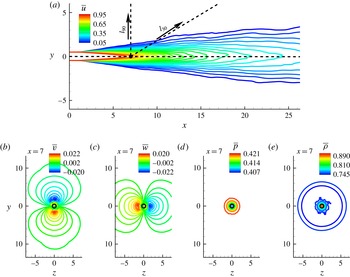
The mean flow features of the jet are shown in figure 2. The mean streamwise velocity, $\overline{u}$ , contours on the $z=0$ plane in figure 2(a) indicate a perfectly expanded axisymmetric jet. The approximate end of the potential core at $x\sim 7$ is marked with a dot. The mean velocity at this centreline location is approximately $92\,\%$ of the jet exit velocity. Two lines originating at this point show $30^{\circ }$ and $90^{\circ }$ rays along which spectral data will be analysed. The mean Cartesian components of velocity, $\overline{v}$ and $\overline{w}$ , on the $x=7$ plane are shown in figures 2(b) and 2(c) respectively. These are an order of magnitude smaller than the streamwise component and are also symmetric about the axis. The mean pressure ( $\overline{p}$ ) and density ( $\overline{{\it\rho}}$ ) contours in figures 2(d) and 2(e) also remain axisymmetric; we take advantage of this property in generating the mean terms of the TFE equation in § 9.

Figure 2.

The mean flow field of the jet: (a), (b), (c), (d) and (e) indicate the $u$ , $v$ and $w$ components of the velocity, and the pressure and density respectively. In (a), two dotted lines inclined at $30^{\circ }$ ( $l_{30}$ ) and $90^{\circ }$ ( $l_{90}$ ) to the jet axis are shown; data along these rays will be analysed in subsequent sections.

The approach has been successfully employed to simulate the Mach 1.3 jet, and detailed comparisons with experimental data may be found in Gaitonde & Samimy (Reference Gaitonde and Samimy2011). For completeness, some results are presented in figure 3. The mean centreline velocity is plotted in (a), taken from Gaitonde & Samimy (Reference Gaitonde and Samimy2011), along with the corresponding experimental value (Samimy et al. Reference Samimy, Kim, Kastner, Adamovich and Utkin2007). The decay rate matches well with the experimental values and provides confidence in the current simulation. It should be noted that since the nozzle exit boundary layer state is unknown, following common practice (Bodony & Lele Reference Bodony and Lele2005), the focus is on the decay after core collapse. Comparison of centreline fluctuation values may also be found in Gaitonde & Samimy (Reference Gaitonde and Samimy2011). Figure 3(b) shows new results comparing computation with experimental far-field sound pressure levels (SPLs) (Samimy et al. Reference Samimy, Kim, Kearney-Fischer and Sinha2010), using the Ffowcs-Williams and Hawkings (FWH) method (Ffowcs-Williams & Hawkings Reference Ffowcs-Williams and Hawkings1969), at $30^{\circ }$ and $94$ jet diameters. The simulations show reasonable agreement with experimental data. Further details, including grid resolution studies, may be found in Gaitonde & Samimy (Reference Gaitonde and Samimy2011).

Figure 3.

(a) Mean streamwise velocity along the centreline of the jet compared with corresponding experimental data (reproduced from Gaitonde & Samimy (Reference Gaitonde and Samimy2011)). (b) Far-field SPLs obtained through the FWH method compared with corresponding experimental data (Samimy et al. Reference Samimy, Kim, Kearney-Fischer and Sinha2010).

Figure 4.

Instantaneous perturbation quantities in the jet shown using contours of the fluctuating component of (a) $u$ and (b) pressure.

For completeness, representative instantaneous fluctuating quantities are shown in figure 4 along a $z=0$ plane. The fluctuating $u$ velocity component is shown in figure 4(a). Both the streamwise and the radial (not shown) velocity fluctuation components are of the same order of magnitude, and the peak instantaneous value of the streamwise fluctuating velocity was found to be approximately $30\,\%$ of the jet exit velocity. The pressure perturbations ( $p^{\prime }$ ) plotted in figure 4(b) show coherent features evolving near the nozzle exit, and represent the signature of axially convecting large-scale structures. Towards the near-acoustic field, patterns consistent with the dilatation (figure 1 c) appear. While the pressure perturbations in the core have significant contributions from the hydrodynamic component, those in the near field are predominantly acoustic due to the implicit filtering by the jet. The perturbation fields indicate that the turbulent core of the jet has a wide range of associated scales and dynamics, including shear layer instability growth, convecting coherent eddies, radiating fields and intense mixing.

The root mean square (RMS) values of fluctuations in the primitive variables along the jet centreline are plotted in figure 5. The peak RMS value of the fluctuating streamwise velocity component reaches approximately $16\,\%$ of the jet exit velocity by approximately $10$ jet diameters downstream. Although lower than the streamwise component, other velocity components also exhibit similar orders of magnitude of RMS values in their corresponding fluctuations. An estimate of the pressure and density fluctuations is also provided in figure 5.

Figure 5.

Root mean square quantities along the centreline of the jet.

3 Doak’s momentum potential theory

A brief discussion of Doak’s method (Doak Reference Doak1989) is first presented. The primary dependent vector field considered for decomposition is the momentum density ( ${\it\rho}\boldsymbol{u}$ ). As described in Doak (Reference Doak1989) and references therein, momentum potential theory possesses several simplifying properties, which make it attractive for application to turbulent flows with acoustic significance.

1. (i) The momentum density, ${\it\rho}\boldsymbol{u}$ , is the primary dependent field, which is expressed as a unique superposition of mean, turbulent, acoustic and thermal components.

2. (ii) The continuity equation, which contains $\boldsymbol{{\rm\nabla}}\boldsymbol{\cdot }{\it\rho}\boldsymbol{u}$ , then yields a Poisson equation comprising only fluctuating mass density and fluctuating scalar potential for the linear momentum density.

3. (iii) For statistically stationary flows, the mean scalar momentum potential is zero.

4. (iv) A decomposition is possible for the mean energy flux into unique turbulent, acoustic and thermal components.

5. (v) The source terms leading to the above mean energy flux can also be categorized into turbulent, acoustic and thermal components, using the TFE equation.

Thus, within the construct of Doak’s theory, a unique definition for the modes, energy flux and its sources is guaranteed.

The details of the method are now summarized. The decomposition of the momentum density is written as

where, again, ${\it\rho}$ and $\boldsymbol{u}$ are the density and particle velocity vector respectively; $\overline{\boldsymbol{B}}$ is the mean solenoidal component, $\boldsymbol{B}^{\prime }$ is the fluctuating solenoidal component and ${\it\psi}^{\prime }$ is the fluctuating scalar potential, whose negative gradient forms the irrotational component of the momentum-density vector. The mean scalar potential $\overline{{\it\psi}}$ for a time-stationary flow is both irrotational and solenoidal, and is assumed to be zero. The above decomposition, coupled with mass conservation for a continuum time-stationary flow, yields a Poisson equation for the fluctuating scalar potential given by

The total irrotational field is further split into a linear combination of acoustic and thermal components, with each obtained from a corresponding Poisson equation. Thus,

Here, ${\it\psi}_{A}^{\prime }$ and ${\it\psi}_{T}^{\prime }$ represent the fluctuating acoustic and thermal components of the irrotational momentum density respectively; $p$ is the thermodynamic pressure, $c^{2}=(\partial p/\partial {\it\rho})_{S}$ is the squared value of the instantaneous local speed of sound and $S$ is the entropy calculated from $S=S_{j}+c_{p}[\ln (T/T_{j})]-R[\ln (p_{j}/p)]$ , where subscript $j$ represents jet exit parameters, while $c_{p}$ is the specific heat at constant pressure and $R$ is the ideal gas constant.

In summary, within the framework of Doak’s theory, the divergence-free component of momentum constitutes the hydrodynamic mode of the flow. The acoustic and thermal modes are components of the irrotational field, driven by density variations resulting from pressure, and entropic fluctuations respectively.

4 Numerical considerations for Helmholtz decomposition

For numerical convenience, many of the main findings are established by considering the $z=0$ half-plane of the LES domain in cylindrical coordinates under the assumption of axisymmetry. The validity of this assumption is verified by performing a full 3-D analysis on a select subset of the full time series, as discussed later in §§ 6 and 8.

With $x$ and $r$ representing the axial and radial directions respectively, an orthogonal coordinate system $({\it\eta},{\it\zeta})$ is introduced, where $r=r({\it\eta})$ and $x=x({\it\zeta})$ . Equation (3.2) can then be expressed as

This equation is discretized to second-order accuracy, yielding a penta-diagonal system which is inverted iteratively using the BiCGSTAB (Van der Vorst Reference Van der Vorst1992) algorithm. A pseudo-time-stepping technique is adopted to ensure convergence of the Poisson solver.

The solenoidal and irrotational components of the momentum density are extracted as follows.

1. (i) The source term for the total irrotational component ${\it\psi}^{\prime }$ in (3.2) is obtained from the LES flow field, and the corresponding Poisson equation is solved. The outer boundaries are far enough away to assume the flow there to be purely irrotational, and hence the fluctuating solenoidal component is negligible. From (3.1), this yields the condition, $({\it\rho}\boldsymbol{u})^{\prime }=-\boldsymbol{{\rm\nabla}}{\it\psi}^{\prime }$ ; ${\it\psi}^{\prime }$ is then integrated along the boundaries to provide a Dirichlet boundary condition for the Poisson solver. At $r=0$ , axisymmetry enforces a zero-gradient Neumann condition for ${\it\psi}^{\prime }$ .

2. (ii) The acoustic part of the irrotational field is obtained by solving the corresponding Poisson equation (3.3) for ${\it\psi}_{A}^{\prime }$ , with its source term again coming from the LES. Assuming temperature fluctuations in the far field to be negligible, the thermal component there is fixed to zero, thus allowing the outer boundary conditions to be specified as ${\it\psi}_{A}^{\prime }={\it\psi}^{\prime }$ . A zero-gradient Neumann condition is used for ${\it\psi}_{A}^{\prime }$ at $r=0$ .

3. (iii) The thermal component of the fluctuating momentum density is obtained from the relationship between acoustic and thermal modes, ${\it\psi}_{T}^{\prime }={\it\psi}^{\prime }-{\it\psi}_{A}^{\prime }$ (see (3.3)).

4. (iv) The mean and the fluctuating solenoidal components are then obtained from (3.1), since $\bar{\boldsymbol{B}}$ is known from the LES.

5 Properties of the decomposed fields

In this section, we describe the qualitative characteristics of each decomposed field, and examine their compliance with known features such as radial decay and directional spectral content. Instantaneous snapshots of the decomposed fields are provided in figure 6. Figure 6(a) shows the contours of the solenoidal fluctuations ( $\Vert \boldsymbol{B}^{\prime }\Vert$ ) (in colour) and the irrotational fluctuations ( $\Vert \boldsymbol{{\rm\nabla}}{\it\psi}^{\prime }\Vert$ ) (in black and white). Different ranges are used because the solenoidal fluctuations are an order of magnitude larger than the maximum irrotational fluctuations. The solenoidal fluctuations closely follow the development of the shear layer and peak in regions of high vorticity. The initial region downstream of the lipline is characterized by shear layer instabilities and eventual collapse of the core ( $6<x<7$ ). The solenoidal fluctuations diminish considerably after $10$ jet diameters downstream as turbulence dies out. Although higher in magnitude than the irrotational field in the turbulent region, the solenoidal fluctuations are damped out rapidly in the radial direction, as discussed further below. The term $\Vert \boldsymbol{B}^{\prime }\Vert$ thus indicates the region of prominent turbulent motion in the free shear layer.

Figure 6.

Instantaneous decomposed momentum-density fluctuations of the jet: (a) $\Vert \boldsymbol{B}^{\prime }\Vert$ contours overlaid with $\Vert \boldsymbol{{\rm\nabla}}{\it\psi}^{\prime }\Vert$ , (b) $\Vert \boldsymbol{{\rm\nabla}}{\it\psi}_{A}^{\prime }\Vert$ , (c) $\Vert \boldsymbol{{\rm\nabla}}{\it\psi}_{T}^{\prime }\Vert$ .

The near field of the jet outside the main turbulent flow is dominated by the irrotational mode, as seen in figure 6(a). This component clearly captures the radiated field, including the highly directional components in the downstream shallow-angle directions. The drop off is also fairly rapid, but not as much as the solenoidal component: the irrotational mode persists to large distances from the core.

Further decomposition of the irrotational component into acoustic and thermal constituents results in figures 6(b) and 6(c) respectively. It should be noted that a larger radial domain has been plotted in the former because the acoustic field remains significant at larger distances from the jet. Although much smaller than the solenoidal component, the highest acoustic mode values also occur in the turbulent region near the axis. Indeed, as shown later, the acoustic response contains a coherent wavepacket in this region, whose dynamics is closely linked to noise radiation. The acoustic mode drops off away from the turbulent region (discussed quantitatively later), but the radiative characteristics of the near-acoustic field are well preserved.

The thermal component shown in figure 6(c) is similar to the solenoidal component in some ways and the acoustic component in others. Like the former, the thermal mode is restricted to the turbulent region, with a rapid drop off in magnitude away from the jet. There is relatively little presence of the thermal mode outside the jet. Overall, however, its magnitude is closer to that of the acoustic mode and approximately an order of magnitude smaller than the solenoidal mode. These fluctuations arise from the entropy and thermal gradients caused due to vorticity and mixing of the cold jet with the ambient fluid, as discussed in detail in § 8. Their relative magnitudes are a consequence of the fact that the present jet is cold, and will change if the jet is heated.

The variation of the hydrodynamic and acoustic modes with radial distance has been documented in the literature. We now use this theoretical knowledge to examine compliance of the decomposed fields. Based on the conservation of energy of concentric waves propagating through a spherical surface, the acoustic component attenuates at a rate proportional to $r^{-2}$ (Mittal Reference Mittal2010). On the other hand, theoretical analyses predict that the hydrodynamic field decays at a higher rate, proportional to $r^{-6}$ (Ribner Reference Ribner1962; Arndt, Long & Glauser Reference Arndt, Long and Glauser1997).

Data were acquired along a ray at $90^{\circ }$ to the jet axis at the end of the mean potential core. The integrated power spectral density (IPSD) of the acoustic field is plotted along with the corresponding reference drop-off curve in figure 7. The acoustic decay rate approaches the $r^{-2}$ curve with increasing radial distance, since the jet tends to behave like a localized point acoustic source emitting purely spherical waves, which is the underlying assumption of the corresponding theoretical prediction.

Figure 7.

Radial variation of the IPSD of $\Vert \boldsymbol{{\rm\nabla}}{\it\psi}_{A}^{\prime }\Vert$ . The theoretical fall-rate curve is included to compare the slopes.

Figure 8.

Radial variation of the IPSD of $B_{r}^{\prime }$ and $\Vert \boldsymbol{B}^{\prime }\Vert$ . The theoretical fall-rate curve $r^{-6}$ is also included along with the curves $r^{-5}$ and $r^{-7}$ to compare the slopes.

The decay rate of the hydrodynamic component is shown in figure 8, using two variables, $B_{r}^{\prime }$ and $\Vert \boldsymbol{B}^{\prime }\Vert$ . In contrast to the acoustic mode, this hydrodynamic rate is only plotted until $r=25$ since beyond this point the hydrodynamic fluctuations are negligible. The $r^{-6}$ behaviour is the best match among $r^{-5}$ , $r^{-6}$ and $r^{-7}$ for both variables plotted in figure 8. The decay rate of $B_{r}^{\prime }$ follows the $r^{-6}$ curve throughout. However, $\Vert \boldsymbol{B}^{\prime }\Vert$ agrees best with $r^{-6}$ in the outer region ( $r>8$ ), but has a slightly lower rate of decay towards the core. We note that the exact decay rates, especially in the turbulent region, can vary slightly from the theoretical curves as they are based on simplified assumptions. The decomposition thus separates out two components from the total fluctuation $({\it\rho}\boldsymbol{u})^{\prime }$ , which attenuate at two different radial decay rates, as anticipated.

The spectrum of the acoustic component is now compared with experimentally observed trends at various polar angles, specifically the F- and G-spectra. By analysing a comprehensive set of experimental data, Tam et al. (Reference Tam, Viswanathan, Ahuja and Panda2008) observed that jet noise spectra followed two universal curves: the F-spectrum along downstream angles, which has a distinct peak at relatively lower frequencies, while the G-spectrum along the sideline directions, with more broadband character. The power spectral density (PSD) of $-\partial {\it\psi}_{A}^{\prime }/\partial x$ at a point nine jet diameters away from the axis on $l_{30}$ (see figure 2) is plotted in figure 9(a) (PSD30) with the F-spectrum by superimposing the peak of the model spectrum on the peak observed in the PSD at $St=0.18$ . The decomposed field is found to follow the model spectrum in the pertinent range of acoustic frequencies and indicates a peak at approximately $St\sim 0.2$ . This is qualitatively consistent with far-field experimental supersonic jet data at similar Mach numbers (Seiner et al. Reference Seiner, Ponton, Jansen and Lagen1992; Viswanathan Reference Viswanathan2004; Tam et al. Reference Tam, Viswanathan, Ahuja and Panda2008). A similar narrow-band character has also been observed in the near field of near-sonic jet LES (Bogey & Bailly Reference Bogey and Bailly2007). The spectrum obtained at $l_{90}=9$ along a $90^{\circ }$ ray from the end of the potential core (PSD90) is plotted with the G-spectrum in figure 9(b). Here, the peak is superimposed at $St=0.24$ . Consistent with the model spectrum, the decomposed acoustic field is broadband in nature.

Figure 9.

The PSD of $-\partial {\it\psi}_{A}^{\prime }/\partial x$ compared with the corresponding model spectrum at $30^{\circ }$ (a) and $90^{\circ }$ (b) from the jet axis.

As a final check on the properties of the predicted solenoidal and irrotational fields, figure 10 compares the time–frequency characteristics of the streamwise component of the decomposed momentum density with those of the pressure perturbation signal obtained at $l_{30}=9$ along a $30^{\circ }$ ray from the end of the potential core. At this location, the signals are not expected to be purely acoustic, but rather to also contain hydrodynamic fluctuations. However, the peak frequency associated with the signal is acoustic in nature. Figure 10(a) shows the scalogram of the pressure perturbation signal ( $p^{\prime }$ ) with non-dimensional time on the horizontal axis and $\text{log}_{10}$ values of the pseudo-frequency on the vertical axis. The quantity plotted is the wavelet coefficient (WC(p)) obtained using a Morlet wavelet. The pseudo-frequency is obtained using the scale to frequency conversion relation for the Morlet wavelet. The $\text{log}_{10}$ scale better resolves the intermittency in the pertinent range of frequencies. For ready reference, $St=0.03$ (lowest), $0.1,0.2,0.3$ and $0.5$ (highest) are marked with dotted lines. The scalogram captures several intermittent events, most of which are centred around frequencies corresponding to $St=0.2$ , which was also found to be the peak acoustic radiation frequency along the $30^{\circ }$ ray in figure 9(a). Experimental evidence (Tam et al. Reference Tam, Viswanathan, Ahuja and Panda2008) also suggests that the acoustic radiation peaks near this frequency at shallow (approximately $30^{\circ }$ ) angles. Apart from the low-intensity events in the acoustic-frequency range, intermittent events with longer duration and higher energy are observed at lower frequencies around and below $St=0.03$ .

Figure 10.

Scalograms of $p^{\prime }$ (a), $B_{x}^{\prime }$ (b), $-\partial {\it\psi}_{A}^{\prime }/\partial x$ (c) and $-\partial {\it\psi}_{T}^{\prime }/\partial x$ (d) at $l_{30}=9$ along a $30^{\circ }$ ray. The dotted horizontal lines indicate $St=0.03,0.1,0.2,0.3$ and $0.5$ from bottom to top. These frequencies are also marked within boxes on the right. Three prominent intermittent events are marked in (c).

The scalogram of $B_{x}^{\prime }$ , WC(H), at this location, shown in figure 10(b), isolates this low-frequency content very clearly, indicating that these energy-rich features are contributed by the turbulent fluctuations. Such low-frequency content in the near field of jets is not considered to be a component of the acoustic mode. Rather it is considered to be ‘non-acoustic’ in nature and is filtered to improve correlation studies between core turbulence and the near-field acoustic signals. Bogey & Bailly (Reference Bogey and Bailly2007) discuss low-frequency peaks in the LES near-field pressure of low-Reynolds-number jets at Mach $0.9$ . They denote this low-frequency component as ‘aerodynamic’ based on the work and terminology of Arndt et al. (Reference Arndt, Long and Glauser1997), who observed this component to be strong near the lipline. The low-frequency content in pressure was also verified in the experimental work of Bogey et al. (Reference Bogey, Barré, Fleury, Bailly and Juvé2007). Consistent with these works, the current decomposition faithfully reproduces the ‘non-acoustic’ low-frequency content in the hydrodynamic component, while the acoustic component is devoid of this content. Although not shown, a comparison of (a) and (b) with the same contour levels confirms that the solenoidal component is free of any significant events above $St=0.08$ .

Figure 10(c) shows the scalogram of $-\partial {\it\psi}_{A}^{\prime }/\partial x$ , WC(A), at the same location. It is evident that this signal incorporates all of the intermittent phenomena found in the pressure perturbation signal in the expected range of acoustic frequencies. Three prominent intermittent events in the acoustic range of frequencies are further discussed in § 6; these are highlighted with dotted curves in figure 10(c) and are marked $\unicode[STIX]{x2460}$ , $\unicode[STIX]{x2461}$ and $\unicode[STIX]{x2462}$ . The contour values of (a) and (c) suggest that the energy content in these events is identical. The radial component of the acoustic momentum-density fluctuations ( $-\partial {\it\psi}_{A}^{\prime }/\partial r$ ) was also analysed and found to exhibit similar intermittent events. The thermal fluctuation scalogram (WC(T)), figure 10(d), confirms the observation that this mode is also attenuated at a higher rate compared with the acoustic component. Indeed, the thermal fluctuations closely follow the features of the solenoidal component, and most of their energy is contained in a lower band of frequencies around $St=0.03$ . Although further discussion of the use of azimuthal planes for the analysis is presented in §§ 6 and 8 by select comparisons with full 3-D analyses, the above results affirm the acceptability of this simplification for Helmholtz decomposition.

Figure 11.

The PSD contours of $({\it\rho}u_{x})^{\prime }$ (a), $B_{x}^{\prime }$ (b), $-\partial {\it\psi}_{A}^{\prime }/\partial x$ (c) and $-\partial {\it\psi}_{T}^{\prime }/\partial x$ (d) obtained at various locations along a $30^{\circ }$ ray. The vertical axis denotes the distance along the ray. The vertical dotted lines mark the frequencies $St=0.1,0.2,0.3$ and $0.5$ from left to right. These frequencies are also marked within boxes at the top of the figure.

The evolution of component modes was analysed at various locations along the $30^{\circ }$ ray using scalograms. The key observations may be summarized as follows. Although a wide range of spatio-temporal scales exists in the turbulent region, the content is primarily solenoidal, while the smaller acoustic component exhibits significant intermittent events in the $St=0.1$ – $St=0.3$ spectral range. At locations further away from the core (as in the results of figure 10), the solenoidal component attenuates rapidly, and the scalograms of $p^{\prime }$ and the acoustic mode $-\boldsymbol{{\rm\nabla}}{\it\psi}_{A}^{\prime }$ become similar to each other, indicating the increasingly acoustic nature of pressure fluctuations outside the turbulent region.

A spectral analysis was performed to understand the evolution of each mode along different polar angles. The main conclusions are highlighted by results along the $l_{30}$ and $l_{90}$ rays. The PSDs of the decomposed modes for the $30^{\circ }$ ray are presented in figure 11, with $\text{log}_{10}$ values of $St$ along the $x$ -axis and the distance along the ray on the $y$ -axis. Thus, horizontal lines indicate spectral content along the ray at the ordinate value, while vertical lines indicate growth or decay with distance of the frequency represented by the abscissa. Again, dotted vertical lines mark the frequencies corresponding to $St=0.1,0.2,0.3$ and $0.5$ from left to right. As a reference, the spectrum of the $x$ -component of the momentum-density fluctuations $({\it\rho}u_{x})^{\prime }$ is presented in figure 11(a). Figure 11(b) shows the contribution of the solenoidal component. This mode clearly contributes to most of the high-energy content in the total signal, especially near the core of the jet. The predominant hydrodynamic energy of the flow is found to have a broadband nature in the frequency range below $St=0.2$ . The inclination of the contours indicates that the highest frequencies are attenuated first. By approximately five jet diameters along this ray, there is relatively little energy between $St=0.2$ and $St=0.5$ . The energy in the acoustic mode, figure 11(c), is enhanced in this region however. The contours indicate a peak around $St=0.2$ at nearly all points of this ray, gaining prominence further away from the core where the hydrodynamic component is attenuated. By approximately $10$ jet diameters, the lower frequencies in the hydrodynamic component are also attenuated and the only remaining contribution to the total fluctuations comes from the acoustic mode with predominant peaks around and below $St=0.2$ . The thermal spectrum shown in figure 11(d) also has features similar to those of the acoustic spectrum near the core of the jet, except that it is attenuated in a manner similar to that of the hydrodynamic mode. The plots thus confirm that the spectra of the three decomposed modes together explain the features in the total signal in a consistent manner.

Figure 12.

The PSD contours of $({\it\rho}u_{r})^{\prime }$ (a), $B_{r}^{\prime }$ (b), $-\partial {\it\psi}_{A}^{\prime }/\partial r$ (c) and $-\partial {\it\psi}_{T}^{\prime }/\partial r$ (d) obtained at various locations along a $90^{\circ }$ ray. The vertical axis denotes the distance along the ray. The vertical dotted lines mark the frequencies $St=0.1,0.2,0.3$ and $0.5$ from left to right. These frequencies are also marked within boxes at the top of the figure.

Results of a similar analysis along the $90^{\circ }$ ray from the end of the mean potential core are provided in figure 12. The radial component of the momentum-density fluctuations $({\it\rho}u_{r})^{\prime }$ is analysed here, as it is most representative of the fluxes along the sideline direction (the axial component yields similar observations however). Figure 12(a–d) shows the PSD contours for the total signal, hydrodynamic, acoustic and thermal fluctuating components respectively. Similarly to the $30^{\circ }$ ray case, most of the high-energy content arises from the turbulent fluctuations near the core, which exhibit a broadband nature. Turbulent fluctuations between $St=0.1$ and $St=0.5$ are found to have a greater longevity along the sideline directions. This is due to the prevalence of relatively random hydrodynamic fluctuations. These propagate in the sideline direction but are effectively filtered out in the downstream direction where more coherent motion dominates. The acoustic fluctuations contribute to most of the total signal spectrum above five jet diameters radially, especially at higher frequencies. In contrast to the $30^{\circ }$ ray case, however, the acoustic spectrum exhibits a broadband nature, which is consistent with the conclusions of Tam et al. (Reference Tam, Viswanathan, Ahuja and Panda2008).

Figure 13.

The irrotational response in the core: (a) the contours of $-\partial {\it\psi}_{A}^{\prime }/\partial x$ and (b) the contours of $-\partial {\it\psi}_{T}^{\prime }/\partial x$ . The insets use a contour range different from the corresponding panels to highlight the near-field characteristics. The dotted inclined line in the inset of (a) marks a $30^{\circ }$ ray to the jet axis from the end of the mean potential core at $x=7$ . The dotted curve in each panel marks the outline of the axial wavepacket.

6 Core dynamics of the acoustic mode

As discussed in § 5, due to the attenuation of the turbulent and thermal components, the features of the decomposed acoustic mode reduce to those of the pressure perturbation signal in the near-acoustic field. However, the structure of the acoustic mode in the core region provides important insights in the context of the wavepacket dynamics discussed in Jordan & Colonius (Reference Jordan and Colonius2013). In this section, we analyse the acoustic mode in the core to visualize the creation of intermittent features which contribute to the peak acoustic spectrum in the downstream direction.

The streamwise components of the irrotational fields, $-\partial {\it\psi}_{A}^{\prime }/\partial x$ and $-\partial {\it\psi}_{T}^{\prime }/\partial x$ , are shown in figure 13. The contours of $-\partial {\it\psi}_{A}^{\prime }/\partial x$ in figure 13(a) indicate that the acoustic mode in the core is a well-defined axially coherent wavepacket, whose spatial extent is outlined by the dotted curve. The wavepacket actually extends well after the collapse of the core ( $x\sim 7$ ) to approximately $10$ jet diameters. However, the envelope qualitatively demarcates only that region of the axially coherent wavepacket (until $x\sim 10$ ) that shows consistent high amplitudes and high periodicity. The prominent features beyond $x\sim 10$ are intermittent in nature, and their formation due to the dynamics of the upstream regions of the wavepacket will be discussed in detail in the following figures. We note that such coherent wavepackets have been educed from the pressure fields of subsonic jets (Freund Reference Freund2001). The decomposed acoustic field, however, provides a better visualization since it is not contaminated by the much larger turbulent component.

An analysis of the evolving simulations indicates that these wavepackets are generated with a dominant periodic nature from the developing shear layer. Although the vortical structures are dissipated downstream, the irrotational fluctuations they create persist and propagate into the near-acoustic and far field of the jet. The inset in figure 13(a) shows the same quantity but is zoomed out to include the near-acoustic field contour levels as well. The same acoustic component that indicated the presence of the axial wavepacket clearly also yields the radiating component. As demonstrated below, this holistic feature of the decomposed field is useful in directly associating the mechanisms in the core with the intermittent features observed in the near-acoustic field. The dotted line in the inset marks a $30^{\circ }$ ray from the end of the mean potential core. The downstream propagating waves are clearly observed to have peak values centred around this ray. The less coherent sideline radiation patterns are visible but not prominently because they have lower amplitudes. An analysis of the transient dataset indicates that the leading region of the acoustic wavepacket primarily emits sideline radiation. This was confirmed by a correlation analysis (not included), which shows that the sideline radiation has peak correlation with the lipline value of the acoustic wavepacket between $x\sim 2$ and $x\sim 5$ . The thermal component of the fluctuating irrotational momentum field shown in figure 13(b) also exhibits a wavepacket nature in the core, but, as shown in the corresponding inset, it does not contribute to the radiated near field.

The scalogram shown earlier at $l_{30}=9$ along the $30^{\circ }$ ray, figure 10(c), indicated three coherent intermittent phenomena occurring around $St=0.2$ . An animation (not included) of the evolving wavepacket in $-\partial {\it\psi}_{A}^{\prime }/\partial x$ contours was used to trace these events back to specific episodes in the core. The results for the most prominent intermittent phenomenon centred around $t\sim 110$ , designated event $\unicode[STIX]{x2461}$ in figure 10(c), are discussed in figure 14. Figure 14(a–d) shows the contours of $-\partial {\it\psi}_{A}^{\prime }/\partial x$ at the indicated time instances, while figure 14(e–h) shows azimuthal vorticity contours ( ${\it\omega}_{{\it\theta}}$ ) at the corresponding instants. The dotted curves in (a–d) track the pertinent feature in the wavepacket as it develops in the downstream direction. Figure 14(a) shows the initial phase of the generation of two adjacent irrotational perturbation zones from the disturbances in the shear layer. These perturbations propagate in the downstream direction, growing in spatial extent and amplitude as seen in (b), around $x=5$ . This axial region in the core is found to consistently experience high amplification of the acoustic wavepacket. The amplified irrotational perturbation zones then coalesce, further intensifying their amplitude and resulting in relatively larger spatial scales, as shown in (c). Such merging and amplification results in a well-defined high-intensity acoustic field, shown in (d), which defines the peak radial extent of the axially coherent wavepacket. This amplification produces a spatially persistent acoustic intermittent event, which propagates into the near field. The internal mechanics of the acoustic wavepacket can thus yield crucial information on the genesis of near-field noise intermittency from the turbulent core.

Figure 14.

Time trace of the core dynamics leading to a prominent intermittent event in the near field; (a–d) indicate the contours of acoustic fluctuations $-\partial {\it\psi}_{A}^{\prime }/\partial x$ and (e–h) indicate the contours of azimuthal vorticity ${\it\omega}_{{\it\theta}}$ . The dotted outline follows the features of interest in (a–d) and (e–h).

The shear layer mechanism accompanying this process is tracked in figure 14(e–h) with the azimuthal vorticity. Figure 14(e) marks a vortical region experiencing an intrusion into the core, as marked by the arrow. This vortex element is accelerated and pushed towards the core as indicated in the succeeding panels (f–h). The correlation between the wavepackets of (a–d) and the azimuthal vorticity in (e–h) highlights the significance of vortex intrusion in creating amplification in the acoustic response field, which in turn yields near-field intermittency. As discussed in § 8, this can create a source for the transport of fluctuating enthalpy by the fluctuating momentum density. In the context of Doak’s analysis (Doak Reference Doak1989), this is equivalent to a deceleration in the solenoidal component of momentum, since the fluid particle is being pushed from a high- to a low-shear region. The consequent reduction of solenoidal fluctuation energy of the fluid volume is manifested as a contribution to the propagated energy flux.

The implication of this intermittent event is felt at a later time in the near-acoustic field. Figure 15 shows contours of $-\partial {\it\psi}_{A}^{\prime }/\partial x$ at a later time of $t=110$ . The dot represents a point at $l_{30}=9$ along a $30^{\circ }$ ray from the end of the mean potential core, where the intermittency of the acoustic mode (event $\unicode[STIX]{x2461}$ ) was analysed in figure 10(c). The amplified acoustic response in the core of the jet discussed above propagates predominantly in the downstream shallow-angle direction and reaches this point at approximately $t=110$ , causing the corresponding intermittency in its scalogram. The spatial features of this near-field event are clearly visible in the contours of $-\partial {\it\psi}_{A}^{\prime }/\partial x$ as a coherent wavefront.

Figure 15.

Contours of $-\partial {\it\psi}_{A}^{\prime }/\partial x$ indicating a coherent event affecting a point (marked by the dot) at nine jet diameters along a $30^{\circ }$ ray from the end of the mean potential core.

Figure 16.

(a) Joint probability distribution contours of ${\it\omega}_{{\it\theta}}^{\prime }$ and $-\partial {\it\psi}_{A}^{\prime }/\partial x$ . (b) Normalized correlation function of ${\it\omega}_{{\it\theta}}^{\prime }$ and $-\partial {\it\psi}_{A}^{\prime }/\partial x$ plotted with non-dimensional lag. (c) Modified signals $A1$ and $V1$ obtained from $-\partial {\it\psi}_{A}^{\prime }/\partial x$ and ${\it\omega}_{{\it\theta}}^{\prime }$ respectively highlighting the peaks in acoustic and vortical signals.

The significance of vorticity in amplifying the acoustic mode, and consequent strong intermittent events, is further analysed statistically. Vortex intrusion into the core results in a sudden peak in the local vorticity, which is manifested as a positive fluctuation in ${\it\omega}_{{\it\theta}}^{\prime }$ . From the discussion of figure 14, it is evident that such an event leads to negative amplification of the local acoustic mode, which should appear as a negative fluctuation in $-\partial {\it\psi}_{A}^{\prime }/\partial x$ . The quadrant analysis described in Wallace (Reference Wallace2016) is used to establish this connection, using ${\it\omega}_{{\it\theta}}^{\prime }$ and $-\partial {\it\psi}_{A}^{\prime }/\partial x$ , and the results are provided in figure 16. The joint probability distribution function (JPDF) of these two signals, using the time history at a typical location in the core ( $(x,r)=(5.5,0.25)$ ), is shown in (a). The horizontal axis represents ${\it\omega}_{{\it\theta}}^{\prime }$ and the vertical axis is $-\partial {\it\psi}_{A}^{\prime }/\partial x$ . It is evident from the symmetric orientation of the JPDF contours in the second and third quadrants that negative variations in vorticity do not influence the acoustic mode in any statistically significant manner. Conversely, the fourth quadrant has a highly skewed distribution, indicating that although intermittent in nature, extreme events in vorticity are positive fluctuations. This clearly leads to negative fluctuations in the acoustic mode, which were found to be intermittently amplified, leading to strong downstream events. This inference can also be summarized by a correlation analysis between ${\it\omega}_{{\it\theta}}^{\prime }$ and $-\partial {\it\psi}_{A}^{\prime }/\partial x$ , as shown in (b). The normalized correlation between these signals is plotted as a function of non-dimensional lag. The peak negative correlation between the vorticity and acoustic signals confirms that the peak fluctuations in these signals are out of phase, as also seen in the JPDF contours. A similar correlation analysis will be utilized in § 8 to statistically establish the source/sink nature of various terms of the TFE transport equation. Finally, we also highlight the relation between these signals in (c). Two quantities, $A1$ and $V1$ , are plotted with non-dimensional time, where

Thus, $\tilde{V1}$ represents the peak fluctuations in ${\it\omega}_{{\it\theta}}^{\prime }$ whenever they are above the RMS value and $\tilde{A1}$ represents the corresponding fluctuation in $-\partial {\it\psi}_{A}^{\prime }/\partial x$ . These signals are normalized by their respective RMS values to highlight the features of interest. The plots of $V1$ and $A1$ clearly show that intermittent positive peaks in vorticity result in negative amplification of the acoustic mode in a consistent manner. Similar observations were also obtained at various other locations within the core.

The decomposed core acoustic field is now explored in further detail to characterize the growth and evolution of the axial wavepacket. The spatio-temporal modulations of this wavepacket are known to be central to the genesis of downstream propagated noise. Cavalieri et al. (Reference Cavalieri, Jordan, Agarwal and Gervais2011) induced temporal modulations in the amplitude and spatial extent (‘jittering’) of a model wavepacket to obtain a good match with sound levels predicted by LES in subsonic jets. Semeraro, Lesshafft & Sandberg (Reference Semeraro, Lesshafft and Sandberg2015) optimally forced a linear wavepacket model in a subsonic jet at $St=0.6$ to recreate downstream-direction response and compared it with the Fourier modes obtained from direct numerical simulation. Likewise, Serré et al. (Reference Serré, Robinet and Margnat2015) modelled the jittering process to recreate radiated sound patterns. Since the current decomposition highlights the internal dynamics of the wavepacket, it offers an opportunity to further investigate factors responsible for this amplification and spatial modulation.

To facilitate a clearer examination of the jittering of the acoustic component from the LES, we first use a chronogram (space–time variation) along the lipline to identify the axial modulation and intermittent amplification of the wavepacket. The space–time signal is then analysed in the spectral domain. The fast Fourier transform along the spatial (axial) coordinate (at each instant) provides the wavenumber ( $k_{x}$ ), while along the time coordinate (fixed space), it provides the frequency ( ${\it\omega}$ ) spectrum. The ratio ${\it\omega}/k_{x}$ yields the convection velocity of the mode. This analysis is again performed on another signal obtained by filtering the original space–time signal within the acoustic band of radiated frequencies. This provides insight into the prominent intermittent events in the core and highlights the most significant ‘jittering’ phenomena responsible for the directional radiation.

The results of performing these steps are shown in figure 17. Various radial locations from $r=0.4$ to $r=1.4$ were examined: the inferences are essentially the same, though the amplitudes vary. The lipline, used also by Freund (Reference Freund2001) and Tinney & Jordan (Reference Tinney and Jordan2008), is an appropriate location, since it encompasses the prominent parts of the wavepacket. Figure 17(a) shows the chronogram of $-\partial {\it\psi}_{A}^{\prime }/\partial x$ along the lipline of the jet. Recurring events are evident at any given location by tracing a vertical line in the plot, as highlighted in the inset. The axial extent of the wavepacket (obtained by examining a horizontal line through the figure) is also seen to be slowly modulated in time. Similar features have been observed in the non-decomposed variables in experiment (Tinney & Jordan Reference Tinney and Jordan2008) and azimuthally averaged computations (Freund Reference Freund2001).

Figure 17.

(a) The $x$ – $t$ plot of $-\partial {\it\psi}_{A}^{\prime }/\partial x$ along the lipline of the jet. (b) Wavenumber–frequency representation of the $x$ – $t$ signal in (a). The horizontal dotted lines mark frequencies with peak energy corresponding to the internal frequency of the wavepacket ( $St=0.38$ ) and the downstream radiation ( $St=0.2$ ). The inclined dotted line represents the prominent convection speed of the wavepacket ( $0.77U_{j}$ ). (c) The filtered $x$ – $t$ signal marked with events in the core leading to prominent near-field intermittency. (d) The spectrum of the filtered signal in (c).

The Fourier transform (FT) of these data is shown in figure 17(b) in the wavenumber–frequency plane. We present only the positive wavenumber domain since the energy contribution of upstream propagating acoustic waves was significantly lower than that of downstream propagating components. The velocity of the wavepacket in the acoustic mode, as indicated by the slope of the FT contours, is approximately $0.77U_{j}$ , which is close to sonic speed. The periodic nature evident in figure 17(a) is manifested as a peak frequency of $St\sim 0.38$ in figure 17(b). This corresponds to the so-called ‘internal’ or ‘average’ frequency (Cavalieri et al. Reference Cavalieri, Jordan, Agarwal and Gervais2011) of the wavepacket. An investigation of the frequency spectrum at each axial location (not included) indicates that the features within the axial locations ranging from $2.5<x<5.5$ contribute the most to this peak frequency; it is in this region that the wavepacket has the greatest radial extent (see figure 13 a). The contours in figure 17(b) also show a weaker peak around $St=0.2$ , which coincides with the downstream peak radiation. This contribution is derived from the region $5.5<x<8.5$ , and corresponds to the influence of the dynamic fluctuations in the core collapse location, which effectively modulate the axial extent of the wavepacket. The higher frequencies in figure 17(b) are contributed by the transition process in the initial shear layer development region close to the nozzle exit. This is due to the fact that the boundary layer exiting the nozzle is very thin and rapidly destabilizes downstream (as can be seen in figure 14 e–h).

Figure 18.

(a) Instantaneous form of the 3-D acoustic wavepacket ( $-\partial {\it\psi}_{A}^{\prime }/\partial x$ ) shown on the $z=0$ half-plane. (b) Instantaneous form of the acoustic wavepacket ( $-\partial {\it\psi}_{A}^{\prime }/\partial x$ ) at the corresponding time instant obtained with one azimuthal slice.

The principal frequency of the wavepacket is found to be higher than the radiated frequency, consistent with the observation of Cavalieri et al. (Reference Cavalieri, Jordan, Agarwal and Gervais2011). It is instructive to further examine the mechanism by which the wavepacket centred around $St=0.4$ radiates at $St=0.2$ . We follow the approach of band-pass filtering the $x$ – $t$ data shown in figure 17(a) around this frequency. For this purpose, we use empirical mode decomposition (EMD), previously utilized for turbulence signals in Agostini & Leschziner (Reference Agostini and Leschziner2014). The band chosen extends from $St=0.1$ to $St=0.3$ . The resulting filtered $x$ – $t$ data and the frequency–wavenumber contents are shown in figures 17(c) and 17(d) respectively. Several core events, designated E1, E2, E3 and E4, can be identified as marked. The first three of these events evolve into the prominent intermittent phenomena observed around $t=47,110$ , and $130$ respectively in the scalogram of figure 10(c), marked as events $\unicode[STIX]{x2460}$ , $\unicode[STIX]{x2461}$ and $\unicode[STIX]{x2462}$ respectively. Core event E2, centred around $t=100$ , is the most prominent, and is responsible for the strong intermittent event in the near-field scalogram at $t=110$ , as discussed earlier. A comparison of the full and filtered signals reveals that all peaks due to wavepacket amplification need not result in a near-field intermittent event. Those peaks occurring between five and nine jet diameters downstream are most efficient in inducing sustained perturbations in the irrotational field. The filtered signal also highlights the modulation of the downstream end of the wavepacket in the range $7<x<10$ . These phenomena together induce the wavepacket to propagate an acoustic field having a relatively narrow-band peak in the downstream direction.

In order to verify that the physical form of the acoustic mode is not significantly affected by the use of an azimuthal slice, we now compare the results from the full 3-D analysis with the axisymmetric calculation. An instantaneous snapshot of the acoustic mode from both calculations is shown in figure 18. The contours of the 3-D axial wavepacket on a $z=0$ slice are shown in (a), while the result with the slice is shown in (b). Both of the calculations clearly yield similar results: all major features of the wavepacket are well represented in both cases and quantitative differences are minor. The comparison is particularly good within the first seven to eight jet diameters, which is the prominent region of the wavepacket, influencing its amplification further downstream. The effects of using a slice on TFE production mechanisms are addressed by comparing the results with corresponding 3-D calculations in § 8.

7 The total fluctuating enthalpy equation

The previous sections (§§ 5 and 6) characterized the physical form and spectral properties of the individual modes in the jet. We now address the second question posed in § 1 on the nature of inter-modal interactions leading to generation and transmission of sound energy from the jet. For this purpose, we adopt Doak’s equation for mean transport of TFE of the flow due to momentum fluctuations (Doak Reference Doak1989). The analysis connects component modes to flow quantities such as vorticity and entropy gradients, which will be shown to be crucial in determining acoustic sources in the jet and relating the intermittent phenomena to the observed sound energy.

A brief description of the TFE equation is now provided. The decomposition of momentum density allows the mean conservation of TFE to be written as a linear superposition of energy fluxes due to fluctuating turbulent, acoustic and thermal components in the flow. The mean transport of the TFE is written as

The total enthalpy per unit mass ( $H$ ) is defined as $H=c_{p}T+\boldsymbol{u}\boldsymbol{\cdot }\boldsymbol{u}/2$ , and $H^{\prime }$ is its total fluctuating component (TFE). The vector ${\bf\alpha}^{\prime }$ is defined as

Here, ${\bf\omega}=\boldsymbol{{\rm\nabla}}\times \boldsymbol{u}$ is the vorticity, $\boldsymbol{{\rm\nabla}}S$ is the entropy gradient and $\overline{\overline{\unicode[STIX]{x1D64E}}}$ is the viscous stress tensor.

The left-hand side of (7.1) represents the mean flux of fluctuating enthalpy carried away by each modal component of the flow. The momentum potential theory thus naturally yields the governing equation for the mean energy flux or the intensity $\overline{H^{\prime }({\it\rho}\boldsymbol{u})^{\prime }}$ , in the form of a linear superposition of uniquely defined components. This helps in understanding the role of acoustic, turbulent and thermal modes in complex flows in carrying the fluctuating enthalpy from turbulent regions into relatively quiescent zones. Each flux automatically vanishes in the absence of the corresponding type of motion.

The right-hand side of (7.1) indicates the various source mechanisms involved in this transport. The vector ${\bf\alpha}^{\prime }$ is termed the net fluctuating ‘acceleration’, which includes contributions from the fluctuations in the vorticity, entropy gradients and viscous stresses in the flow. These terms provide insight into the production and dissipation of the TFE due to interaction of momentum fluctuations with the ‘acceleration’ vector ${\bf\alpha}^{\prime }$ . This interaction represents the rate of production of TFE per unit volume due to the Coriolis component of ‘acceleration’, which is a result of vorticity, as well as interaction of momentum fluctuations with the fluctuating dissipative forces per unit mass due to entropy gradients and viscosity. By applying the decomposition of the momentum fluctuations, the role of each mode in the production or dissipation of TFE due to its interaction with the ‘acceleration’ vector can be studied. The contribution of the viscous stresses to the source term is found to be orders of magnitude smaller than those from vorticity and entropy gradients, which is anticipated for this relatively high-Reynolds-number jet. The last term on the right-hand side, $({\it\rho}T)^{\prime }\partial S^{\prime }/\partial t$ , is dissipative in nature and is analogous to thermal diffusion due to entropy fluctuations.

The TFE ( $H^{\prime }$ ) can be further split into acoustic ( $H_{A}^{\prime }$ ), thermal ( $H_{T}^{\prime }$ ) and turbulent ( $H_{B}^{\prime }$ ) component fluctuations based on Jenvey (Reference Jenvey1989). The rationale behind this is to define all components of the TFE associated with pressure fluctuations as acoustic and those components associated with entropy fluctuations as entropic. The remaining component, which is solenoidal, is either vortical or turbulent. In the interest of completeness, the following discussion, based on Doak (Reference Doak1989), summarizes this decomposition.

For a time-stationary flow, the total enthalpy ( $H$ ) per unit mass can be split into mean and fluctuating quantities as

where $h=c_{v}T+p/{\it\rho}$ is the static enthalpy, with $c_{v}$ being the specific heat at constant volume, and $\boldsymbol{m}={\it\rho}\boldsymbol{u}$ is the momentum-density vector. Using the thermodynamic state relationships, ${\it\rho}={\it\rho}(p,S)$ and $h=h(p,S)$ , the time derivative of total enthalpy can be defined as

where ${\it\rho}_{p}=(\partial {\it\rho}/\partial p)_{S}$ and ${\it\rho}_{S}=(\partial {\it\rho}/\partial S)_{p}$ . In the above, the time derivative of the momentum density ( $\boldsymbol{m}$ ) has been replaced by the linear combination of the acoustic, hydrodynamic and thermal components. The rate of change of density fluctuation is also split into its components, which depend on pressure and entropy fluctuations. This facilitates the association of components of $H^{\prime }$ with specific modes. By representing $H=\overline{H}+H_{B}^{\prime }+H_{A}^{\prime }+H_{T}^{\prime }$ (where $H_{B}^{\prime },H_{A}^{\prime }$ and $H_{T}^{\prime }$ correspond to the hydrodynamic, acoustic and thermal components of the TFE respectively) and equating each term to corresponding components in (7.4), the individual components of the TFE are obtained as

where $h_{p}=(\partial h/\partial p)_{S}$ and $h_{S}=(\partial h/\partial S)_{p}$ . For an ideal gas following $p=(c_{p}-c_{v})T$ , with a constant ratio of specific heats ${\it\gamma}=c_{p}/c_{v}$ and speed of sound defined as $c=({\it\gamma}p/{\it\rho})^{1/2}$ , the above expressions can be integrated, neglecting products of fluctuations, to yield first-order approximations for the corresponding components of the TFE as follows: where the Mach number vector is defined as $\boldsymbol{M}\equiv \boldsymbol{u}/c$ .

8 Behaviour of source mechanisms in the TFE

We now use (7.1) to analyse the various flux and source terms with the goal of understanding the sound generation process in the jet, specifically the events that accompany the entrainment episode identified in § 6 above. Previous works (Daviller et al. Reference Daviller, Jordan and Comte2009; Jordan et al. Reference Jordan, Daviller and Comte2013) have explained the behaviour of the mean flux and source terms of (7.1) for model wavepacket problems. Here, we first consider the instantaneous behaviour of the source terms, to gather insight into the dynamics between momentum and shear-induced vorticity and associated entropy gradients. We also consider the contribution of dissipation mechanisms due to entropy fluctuations to the TFE budget.

The various source terms in (7.1) are represented as dot products (interaction) between the decomposed components of the fluctuating momentum density and the fluctuating ‘acceleration’ vector ${\bf\alpha}^{\prime }$ . Whenever these vectors are non-orthogonal, a source term is activated leading to the production/destruction of TFE and its subsequent transport. The mutual orthogonality of these vector fields results in zero sources. Doak described such a scenario as ‘local fluctuating dynamic equilibrium’ (Doak Reference Doak1989). Under this condition, a silent flow is obtained where turbulent, acoustic and thermal intensities nullify the net effect in any given volume element of the fluid so that the momentum fluctuations do not result in any inflow or outflow of energy. When these vector fields are non-orthogonal, a mean energy transport defined by (7.1) is generated, resulting in acoustic radiation from the jet. The current analysis of the relevant instantaneous quantities elucidates the precise mechanisms in a developing shear layer which prevents the existence of a ‘local fluctuating dynamic equilibrium’ condition.

Before going into the details of the source mechanisms, we briefly describe the nature of the ‘acceleration’ vector and the associated physical phenomena. The fluctuating ‘acceleration’ vector has components from the fluctuating Coriolis acceleration, fluctuating entropy gradients and viscous stresses. To separate the associated mechanisms, we consider each component individually by denoting ${\bf\alpha}^{\prime }={\bf\alpha}_{1}^{\prime }+{\bf\alpha}_{2}^{\prime }$ , where ${\bf\alpha}_{1}^{\prime }=({\bf\omega}\times \boldsymbol{u})^{\prime }$ and ${\bf\alpha}_{2}^{\prime }=-(T\boldsymbol{{\rm\nabla}}S+[1/({\it\rho}Re)]\boldsymbol{{\rm\nabla}}\boldsymbol{\cdot }\overline{\overline{\unicode[STIX]{x1D64E}}})^{\prime }$ . As noted earlier, the viscous stress contribution to ${\bf\alpha}_{2}^{\prime }$ is negligible compared with the fluctuating entropy gradients, and hence these two components are combined together. The features of the components of ${\bf\alpha}^{\prime }$ are shown in figure 19. An instantaneous snapshot of vorticity ( ${\it\omega}_{{\it\theta}}$ ) is shown in figure 19(a) for reference to indicate the development of the shear layer and mixing. Figures 19(b) and 19(c) show the instantaneous contours for ${\bf\alpha}_{1}^{\prime }$ and ${\bf\alpha}_{2}^{\prime }$ respectively. Major fluctuations in the Coriolis acceleration occur in regions of high vorticity, typically tracing the shear layer roll-up in regions of higher velocity. They thus identify intrusion of vortices into the core of the jet. As a result, the peak values are generally observed closer to the inner side of the developing shear layer, as seen in figure 19(b). Once the core collapses, the intense mixing spreads out this component. The term ${\bf\alpha}_{2}^{\prime }$ closely represents the entrainment process in the shear layer and traces the ingestion of the ambient fluid into the core. The shear and temperature gradients involved in this process induce fluctuations in entropy gradients, which can be seen in figure 19(c). The traces of this process highlight the Kelvin–Helmholtz instability patterns in the free shear layer. While Coriolis acceleration is considered to be a production term, the fluctuations in entropy gradients and viscous stresses are decelerations due to dissipative mechanisms (Doak Reference Doak1989).

Figure 19.

Contours of (a) vorticity ${\it\omega}_{{\it\theta}}$ , and magnitudes of (b) ${\bf\alpha}_{1}^{\prime }$ and (c) ${\bf\alpha}_{2}^{\prime }$ .

The relative magnitudes of ${\bf\alpha}_{1}^{\prime }$ and ${\bf\alpha}_{2}^{\prime }$ can be considered as an implication of Crocco’s equation, which can also be interpreted as a coupling of entropic and vorticity modes. While ${\bf\alpha}_{1}^{\prime }$ represents the ‘rotational’ or vortex structures in the vorticity, ${\bf\alpha}_{2}^{\prime }$ highlights the shear. We note that this balance will be different in the case of hot jets. If the heating is assumed not to have a significant impact on the vortex structures, the term ${\bf\alpha}_{1}^{\prime }$ will remain similar. However, higher temperature gradients in the shear layer can be expected to intensify the entropy gradients in the entrainment streaks, thus modifying ${\bf\alpha}_{2}^{\prime }$ .

The interaction of the ‘acceleration’ and momentum density leads to various source mechanisms for the TFE, of which the most prominent ones are discussed below in detail. The non-orthogonality of fluctuations in the solenoidal component of the momentum density and the ‘acceleration’ term is the most significant interaction. In the following, we discuss the interaction of the vector fields $\boldsymbol{B}^{\prime }$ and ${\bf\alpha}^{\prime }$ (which comprises ${\bf\alpha}_{1}^{\prime }$ and ${\bf\alpha}_{2}^{\prime }$ ). An instantaneous snapshot of these vector fields is provided in figure 20, to highlight their relative orientation. The snapshot is typical of the vortex intrusion and entrainment process in the shear layer, as observed in animations of the corresponding quantities, and is confirmed through a subsequent statistical analysis of the respective source terms.

Figure 20.

Interaction of the solenoidal fluctuations with ‘acceleration’ terms. In (a), the solid (black) vectors indicate the vector field $\boldsymbol{B}^{\prime }$ and the dotted (red) vectors indicate the vector field ${\bf\alpha}_{1}^{\prime }$ . The contours represent the dot product of these two fields. In (b), the solid vectors (black) indicate the vector field $\boldsymbol{B}^{\prime }$ and the dotted vectors (red) indicate the vector field ${\bf\alpha}_{2}^{\prime }$ . The contours represent the dot product of these two fields. In each panel, the inset zooms into the region marked by the dotted square to highlight the orientation of the vector fields.

We first detail the nature of the TFE source due to solenoidal–Coriolis acceleration interaction, $\boldsymbol{B}^{\prime }\boldsymbol{\cdot }{\bf\alpha}_{1}^{\prime }$ . This is shown in figure 20(a), where the solid (black) arrows denote the solenoidal fluctuating momentum $\boldsymbol{B}^{\prime }$ , while the dotted (red) arrows indicate the fluctuating Coriolis acceleration ( ${\bf\alpha}_{1}^{\prime }$ ) vector fields respectively. It should be noted that the size of the arrows has been chosen for clarity and is not proportional to the magnitude of the vector. The background contours indicate the dot product of these two vector fields and highlight regions of strong interactions leading to sources or sinks. It should also be noted that the discussion involves the fluctuating components of the corresponding vector fields. The following inferences are readily apparent.

1. (i) The solenoidal fluctuations are indicative of the curl of the velocity vector in the shear layer and identify the rotational nature of the vortical features.

2. (ii) The two vector fields, $\boldsymbol{B}^{\prime }$ and ${\bf\alpha}_{1}^{\prime }$ , are seen to be near-orthogonal away from the vicinity of the lipline at $r=0.5$ . Hence, major sources of the TFE are localized around the lipline.

3. (iii) A positive source is created when the vector fields are aligned in opposite directions, as can be seen near the coordinates $(x,r)=(4.4,0.3)$ , marked by the dotted square. This region is also shown in the inset; it highlights negative fluctuations in $\boldsymbol{B}$ and positive fluctuations in ${\bf\alpha}_{1}$ .

4. (iv) The orientation of $\boldsymbol{B}^{\prime }$ in this positive source region is the result of transfer of a fluid element from a region of high shear into the potential core. This induces negative fluctuations in the solenoidal component, interpreted as the deficiency of momentum, due to intrusion of the low-velocity fluid into the high-speed core of the jet.

5. (v) The radial and axial components of the Coriolis acceleration term ( ${\bf\omega}\times \boldsymbol{u}$ ) in this region have positive fluctuations ( ${\bf\alpha}_{1}^{\prime }$ ) because a vortical element pushed into the core experiences a higher velocity in the core while being accelerated.

6. (vi) Hence, within this source region, ${\bf\alpha}_{1}^{\prime }$ is seen to be aligned mainly in the ‘north-east’ (radial and axial components of ${\bf\alpha}_{1}$ experience positive fluctuations) direction since it is also expected to be orthogonal to the velocity vector (points south-east generally, not shown). On the other hand, $\boldsymbol{B}^{\prime }$ is aligned along the ‘south-west’ direction (radial and axial components of $\boldsymbol{B}$ experience negative fluctuations, which is the effect of intrusion of vortices into the core).

Thus, the intrusion of high vortical regions towards the core activates the turbulent source term causing mean energy flow through momentum fluctuations.

Figure 21.

(a)–(d) Correlation of components of $\boldsymbol{B}^{\prime }$ and ${\bf\alpha}_{1}^{\prime }$ as indicated, plotted with lag. (e) Histogram of the source term $-\boldsymbol{B}^{\prime }\boldsymbol{\cdot }{\bf\alpha}_{1}^{\prime }$ .

The term ${\bf\alpha}_{2}^{\prime }$ is dominated by fluctuations in entropy gradients. Its interaction with the solenoidal momentum fluctuations is shown in figure 20(b). The solid arrows denote the solenoidal fluctuating momentum $\boldsymbol{B}^{\prime }$ and the dotted arrows indicate the fluctuating entropy gradient and viscous stress acceleration ( ${\bf\alpha}_{2}^{\prime }$ ) vector fields. The contours again represent the dot product of the two vector fields. The following observations are apparent.

1. (i) Contrary to the Coriolis acceleration component, the entropy gradients primarily produce sinks. Regions indicating prominent entrainment streaks in figure 19(c) are found to be strong sinks in figure 20(b).

2. (ii) The negative solenoidal momentum fluctuations (the axial and radial components of $\boldsymbol{B}^{\prime }$ ) now act on the similarly aligned entropy gradient fluctuation vector (due to the negative nature of components of ${\bf\alpha}_{2}^{\prime }$ ), producing a sink.

3. (iii) Within the entrainment streaks, entropy gradients are heightened due to sustained shearing and temperature gradients due to mixing. A fluid element moving towards the core along these streaks experiences positive fluctuations of entropy gradients (due to the positive nature of axial and radial components of $\left(T\boldsymbol{{\rm\nabla}}S\right)^{\prime }$ ). The definition of ${\bf\alpha}_{2}^{\prime }$ involving the negative of this fluctuation gradient causes the two vector fields ( $\boldsymbol{B}^{\prime }$ and ${\bf\alpha}_{2}^{\prime }$ ) to be more likely to be similarly aligned when entrainment occurs.

The mixing induced entropy generation thus dissipates the energy that would have otherwise been carried away by the momentum fluctuations.

The relative alignment of the vector fields $\boldsymbol{B}^{\prime }$ , ${\bf\alpha}_{1}^{\prime }$ and ${\bf\alpha}_{2}^{\prime }$ shown in figure 20 is very typical, i.e. the intrusion of vortical regions into the core consistently produces a positive source term due to the opposite alignment of $\boldsymbol{B}^{\prime }$ and ${\bf\alpha}_{1}^{\prime }$ . Conversely, the entrainment streaks result in negative source terms inside the lipline, dissipating TFE due to similar alignment of $\boldsymbol{B}^{\prime }$ and ${\bf\alpha}_{2}^{\prime }$ . In order to ensure that these observations are statistically valid, correlation analysis was performed, and some typical results are summarized below. In the following analysis, the correlation function of two variables, e.g. $f_{1}$ and $f_{2}$ , is represented in the corresponding figures as $\langle f_{1},f_{2}\rangle$ . If $f_{1}$ and $f_{2}$ exhibit a similar nature of fluctuations, a high positive correlation peak is observed. Out of phase or opposite nature of fluctuations results in a negative peak.

Figure 22.

(a)–(d) Correlation of components of $\boldsymbol{B}^{\prime }$ and ${\bf\alpha}_{2}^{\prime }$ as indicated, plotted with lag. (e) Histogram of the source term $-\boldsymbol{B}^{\prime }\boldsymbol{\cdot }{\bf\alpha}_{2}^{\prime }$ .

The turbulent production term, $-\boldsymbol{B}^{\prime }\boldsymbol{\cdot }{\bf\alpha}_{1}^{\prime }$ , is explored in figure 21, which is obtained at $(x,r)=(2.7,0.4)$ . Figure 21(a) shows the correlation between the two components of $\boldsymbol{B}^{\prime }$ . The high positive correlation at zero lag indicates that this vector field has similar variations (both negative) whenever vortical intrusion occurs into the core. This is because the intruding vortical region brings in fluid with low momentum and high vorticity into the core of the jet. This ensures that its south-west alignment, discussed in figure 20(a), is statistically consistent. Similarly, the high positive correlation of the components of ${\bf\alpha}_{1}^{\prime }$ in (b) also indicates that this vector field has similar variations in both its components (both positive), hence resulting in a north-east direction, as shown in figure 20(a). This is because the vortical element, due to its high vorticity, has a higher Coriolis acceleration compared with the core. The result of these signs of fluctuations on the dot product of these vector fields can be seen in (c) and (d). The strong negative peaks in correlations between the dot-product terms $(B_{x}^{\prime },{\it\alpha}_{1x}^{\prime })$ and $(B_{r}^{\prime },{\it\alpha}_{1r}^{\prime })$ show that they are out of phase. Therefore, the net value of the dot product is mostly negative, which makes the turbulent production term of TFE, $-\boldsymbol{B}^{\prime }\boldsymbol{\cdot }{\bf\alpha}_{1}^{\prime }$ , predominantly positive. The histogram of this term is shown in (e), with the horizontal axis representing the bin-centre value of the production term and the vertical axis representing the fraction of occurrences obtained as the ratio of the number of occurrences within a given bin ( $N_{bin}$ ) to the total number of samples ( $N$ ). The histogram clearly shows the positive nature of the term $-\boldsymbol{B}^{\prime }\boldsymbol{\cdot }{\bf\alpha}_{1}^{\prime }$ , indicating that it is a statistically significant source of TFE.

The entrainment streaks are primary dissipation regions of TFE inside the lipline of the jet. Figure 22 shows a typical result for the correlation analysis of the vector fields $\boldsymbol{B}^{\prime }$ and ${\bf\alpha}_{2}^{\prime }$ obtained at $(x,r)=(2.2,0.4)$ . High positive correlation peaks are observed for the components of the corresponding vector fields $\boldsymbol{B}^{\prime }$ (a) and ${\bf\alpha}_{2}^{\prime }$ (b). The associated vector fields thus have similar variations in their components. Components of $\boldsymbol{B}^{\prime }$ primarily experience negative values inside the core, as described above. The same is true for the components of ${\bf\alpha}_{2}^{\prime }$ , since they are defined as the fluctuations in the negative spatial gradient of entropy. The peak correlations of $(B_{x}^{\prime },{\it\alpha}_{2x}^{\prime })$ and $(B_{r}^{\prime },{\it\alpha}_{2r}^{\prime })$ are positive, indicating that these components are in phase. Hence, the dot product of these vector fields (given by $B_{x}^{\prime }{\it\alpha}_{2x}^{\prime }+B_{r}^{\prime }{\it\alpha}_{2r}^{\prime }$ ) is mostly positive, resulting in a negative source term for TFE, due to $-\boldsymbol{B}^{\prime }\boldsymbol{\cdot }{\bf\alpha}_{2}^{\prime }$ . It was also noted that due to the high spatial gradients of entropy in the radial direction, compared with the axial direction, the term $B_{r}^{\prime }{\it\alpha}_{2r}^{\prime }$ is more influential in creating this dissipation for the TFE. The histogram of $-\boldsymbol{B}^{\prime }\boldsymbol{\cdot }{\bf\alpha}_{2}^{\prime }$ shown in (e) confirms that this is a negative source.

Figure 23.

Correlation of $B_{x}^{\prime }$ and ${\it\alpha}_{2r}^{\prime }$ with the fluctuating vorticity, at locations above and below the lipline of the jet.

A similar analysis showed that the interaction of the fluctuating solenoidal component and entropy gradients can act as a source of TFE outside the shear layer (although not as intense as the source mechanism created due to vortex intrusion into the core). This mechanism is explained as follows. While the vortices are ejected out from the shear layer into the low-velocity ambient fluid, the resulting heightened entropy gradients cause negative fluctuations ${\bf\alpha}_{2}^{\prime }$ , outside the lipline of the jet. However, the fluctuating solenoidal component $\boldsymbol{B}^{\prime }$ in these ejected vortices is positive outside the lipline. Such events introduce localized packets of relatively high vorticity and high momentum into the ambient stagnant fluid surrounding the jet. This results in predominantly out of phase variations in $\boldsymbol{B}^{\prime }$ (positive) and ${\bf\alpha}_{2}^{\prime }$ (negative), creating a positive source of TFE, $-\boldsymbol{B}^{\prime }\boldsymbol{\cdot }{\bf\alpha}_{2}^{\prime }$ , outside the lipline of the jet.

This dual behaviour of the turbulent–entropy-gradient interaction ( $-\boldsymbol{B}^{\prime }\boldsymbol{\cdot }{\bf\alpha}_{2}^{\prime }$ ) is confirmed in the plots shown in figure 23. The aim is to establish correlation of the source/sink characteristics of $-\boldsymbol{B}^{\prime }\boldsymbol{\cdot }{\bf\alpha}_{2}^{\prime }$ above and below the lipline of the jet. For this, the components of the fluctuating solenoidal and acceleration fields are correlated with the fluctuating azimuthal vorticity above and below the lipline of the jet at a given axial location. The results presented here are obtained at $(x,r)=(2.2,0.4)$ , which is below the lipline, and $(x,r)=(2.2,0.6)$ , which is above the lipline. The ejection of vortices to regions above the lipline and entrainment of vorticity into the core induces a positive fluctuation in azimuthal vorticity, and hence ${\it\omega}_{{\it\theta}}^{\prime }$ is positive during such instances. By correlating the components of $\boldsymbol{B}^{\prime }$ and ${\bf\alpha}_{2}^{\prime }$ with ${\it\omega}_{{\it\theta}}^{\prime }$ , the dependence of these vector fields on entrainment and ejection events of vortices can be statistically defined. Figure 23(a) shows the peak negative correlation of ${B_{x}}^{\prime }$ with ${\it\omega}_{{\it\theta}}^{\prime }$ at a point below the lipline. This indicates that entrainment of vorticity into the core leads to negative fluctuations in the solenoidal component, ${B_{x}}^{\prime }$ , consistent with the description of figure 20(b); ${B_{r}}^{\prime }$ was also seen to have similar results. The correlation of ${\it\alpha}_{2r}^{\prime }$ with ${\it\omega}_{{\it\theta}}^{\prime }$ also has a peak negative correlation at the location below the lipline, as seen in (b). Here, ${\it\alpha}_{2r}^{\prime }$ was chosen for representation because it is the prominent component of ${\bf\alpha}_{2}^{\prime }$ . Therefore, entrainment of vorticity into the core also leads to negative fluctuations in the acceleration vector ${\bf\alpha}_{2}^{\prime }$ . Thus, the term $-\boldsymbol{B}^{\prime }\boldsymbol{\cdot }{\bf\alpha}_{2}^{\prime }$ is a negative source for TFE inside the lipline of the jet, as explained in figure 20(b).

Figure 24.

(a) Instantaneous net turbulent source term, $-\boldsymbol{B}^{\prime }\boldsymbol{\cdot }{\bf\alpha}^{\prime }$ , due to interaction of the solenoidal fluctuations with ‘acceleration’ terms. (b–d) Mean turbulent source terms of the TFE transport equation as indicated. The horizontal dotted lines mark the lipline of the jet.

The corresponding analysis at the location above the lipline is shown in (c) and (d). From (c), one deduces that the positive peak correlation between solenoidal and vortical fluctuations indicates the positive nature of $\boldsymbol{B}^{\prime }$ in the vortices ejected out of the shear layer. At the same time, (d) indicates that these regions experience negative fluctuations, ${\bf\alpha}_{2}^{\prime }$ , due to the spatial entropy gradients. This out of phase relationship between $\boldsymbol{B}^{\prime }$ and ${\bf\alpha}_{2}^{\prime }$ leads to a positive source for TFE at locations above the lipline.

To summarize the net effect of the turbulent production term, the sum of $-\boldsymbol{B}^{\prime }\boldsymbol{\cdot }{\bf\alpha}_{1}^{\prime }$ and $-\boldsymbol{B}^{\prime }\boldsymbol{\cdot }{\bf\alpha}_{2}^{\prime }$ is plotted in figure 24(a) in the form of contours of $-\boldsymbol{B}^{\prime }\boldsymbol{\cdot }{\bf\alpha}^{\prime }$ . The axis ranges are maintained the same as in figure 20. The regions of vortex intrusion and entrainment streaks remain sources and sinks respectively of TFE. The mean behaviour of these terms also shows their consistent nature. The mean value of $-\boldsymbol{B}^{\prime }\boldsymbol{\cdot }{\bf\alpha}_{1}^{\prime }$ shown in (b) indicates that this term is a prominent source of TFE within the shear layer. The second term, $-\boldsymbol{B}^{\prime }\boldsymbol{\cdot }{\bf\alpha}_{2}^{\prime }$ , results in a sink which becomes stronger towards the centreline of the jet, as shown in (c). This strengthening of the sink is due to increasing spatial entropy gradients as the fluid is continually sheared along the entrainment streaks. The positive-source nature of this term is also visible outside the lipline of the jet, which is consistent with the previous discussion based on correlation analysis. The net result of interaction between various turbulent source terms is shown in (d), which clearly identifies a prominent source region of TFE flanking the lipline of the jet, and a sink region towards the centreline of the jet. The mean source/sink nature of all of the terms in the TFE transport equation will also be discussed comprehensively in § 9.

Figure 25.

(a) Transfer of a fluid element with high vortical fluctuations from the shear layer into the core shown schematically. This is associated with release of energy from this fluid element which is carried away in the form of TFE flux by momentum-density fluctuations. (b) The entrainment streaks developing in the shear layer shown schematically. These regions exhibit high entropy gradients and are prominent regions where TFE is dissipated.

The schematic in figure 25 summarizes the above discussion. The solenoidal fluctuations resulting from the shear layer roll-up intrude into the potential core as shown in (a), setting up a scenario for production of TFE which is propagated by the fluctuating momentum density into the near field. This contributes to the observed acoustic signature of the jet. Conversely, the ingestion of the ambient fluid into the core highlighted by the entrainment streaks in (b) causes regions of high gradients of entropy. These streaks are the prominent regions in the core where TFE is dissipated out, thus acting as sinks.

Figure 26.

Instantaneous TFE source terms indicated along with vorticity. The contours represent ${\it\omega}_{{\it\theta}}$ (a), $-\boldsymbol{B}^{\prime }\boldsymbol{\cdot }{\bf\alpha}^{\prime }$ (b), $\boldsymbol{{\rm\nabla}}{\it\psi}_{A}^{\prime }\boldsymbol{\cdot }{\bf\alpha}^{\prime }$ (c) and $\boldsymbol{{\rm\nabla}}{\it\psi}_{T}^{\prime }\boldsymbol{\cdot }{\bf\alpha}^{\prime }+({\it\rho}T)^{\prime }\partial S^{\prime }/\partial t$ (d).

We now summarize all of the source terms of (7.1) in figure 26. At this point, the effects of ${\bf\alpha}_{1}^{\prime }$ and ${\bf\alpha}_{2}^{\prime }$ are not separately considered. The quantities plotted include the interaction of the corresponding component of momentum density (solenoidal, acoustic and thermal) with the ‘acceleration’ vector ${\bf\alpha}^{\prime }$ . Instantaneous vorticity ( ${\it\omega}_{{\it\theta}}$ ) contours are again shown in figure 26(a) for reference. Figure 26(b) shows the instantaneous source caused by the turbulent production term ( $\boldsymbol{B}^{\prime }\boldsymbol{\cdot }{\bf\alpha}^{\prime }$ ). This quantity is positive in the majority of the spreading shear layer region, which is dominated by rotational structures and has sinks in localized entrainment regions. The production term due to acoustic fluctuations shown in figure 26(c) ( $\boldsymbol{{\rm\nabla}}{\it\psi}_{A}^{\prime }\boldsymbol{\cdot }{\bf\alpha}^{\prime }$ ) is relatively weak and comprises sources only in the entrainment region due to interaction with entropic fluctuations. This shows that the irrotational field has negligible interaction with the Coriolis acceleration induced by the rotational nature of the flow. However, it interacts more with the entropy gradients in the entrainment streaks, in particular the positive regions of the acoustic wavepacket. This results in opposite alignment of $-\boldsymbol{{\rm\nabla}}{\it\psi}_{A}^{\prime }$ and ${\bf\alpha}_{2}^{\prime }$ , which in turn creates a positive source due to the negative sign on this term in (7.1).

Apart from the interactions of the ‘acceleration’ term and the momentum-density fluctuations, an additional dissipation term, $({\it\rho}T)^{\prime }\partial S^{\prime }/\partial t$ , is involved in (7.1) which is analogous to thermal diffusion (Doak Reference Doak1989) due to the rate of change of entropic fluctuations. This term is considerably larger than the sinks created due to the interaction of the thermal momentum fluctuations with the ‘acceleration’ terms ( $\boldsymbol{{\rm\nabla}}{\it\psi}_{T}^{\prime }\boldsymbol{\cdot }{\bf\alpha}^{\prime }$ ), and hence their combined value is shown in figure 26(d). As the contour values suggest, this is the most prominent sink in the cold jet. These sink regions also follow the entrainment regions discussed earlier in figure 20(b). The source/sink characteristics of each of the terms discussed above are consistent with Doak’s theoretical predictions (Doak Reference Doak1989). Although the jet studied is cold, some comments may be made for heated jets. If the result of heating is assumed to primarily intensify the mixing and entropy gradients ( ${\bf\alpha}_{2}^{\prime }$ ), and have a lesser impact on the vortex strength, it could result in stronger sinks inside and stronger sources outside the lipline for the TFE. If the outer sources are more efficient in transmitting TFE, a potentially louder jet may result. However, heating can also intensify the dissipation term $({\it\rho}T)^{\prime }\partial S^{\prime }/\partial t$ in (7.1). Hence, the net production of TFE depends on the new balance between these counter-acting mechanisms.

Figure 27.

(a) Instantaneous turbulent source mechanism of TFE, $-\boldsymbol{B}^{\prime }\boldsymbol{\cdot }{\bf\alpha}^{\prime }$ , from 3-D analysis. (b) Instantaneous turbulent source mechanism of TFE, $-\boldsymbol{B}^{\prime }\boldsymbol{\cdot }{\bf\alpha}^{\prime }$ , from axisymmetric analysis. (c) Time trace of $-\boldsymbol{B}^{\prime }\boldsymbol{\cdot }{\bf\alpha}^{\prime }$ from the 3-D and axisymmetric analyses at $(x,r)=(5.3,0.4)$ on the symmetry plane (as indicated by the dots in (a) and (b)).

The validity of the above analysis of events in an azimuthal plane is established by considering select results performed with the full 3-D dataset. An instantaneous snapshot of the turbulent production mechanism of TFE, $-\boldsymbol{B}^{\prime }\boldsymbol{\cdot }{\bf\alpha}^{\prime }$ , for the 3-D case is shown in figure 27(a). The corresponding result for the axisymmetric calculation on the azimuthal plane is shown in (b). Both of the analyses yield consistent results in terms of the nature of the source, highlighting several TFE production regions due to vortex intrusion. A few sinks due to entrainment are also visible. Slight variations in the magnitude are found closer to the axis, but their relative signs remain the same. Figure 27(c) shows the time trace of this quantity for the 3-D and axisymmetric calculations at $(x,r)=(5.3,0.4)$ on the symmetry plane (as indicated by the dots in (a) and (b)). Both of the calculations predict similar trends in the behaviour of the source mechanism, although the axisymmetric version occasionally misses the peak values obtained in the full 3-D version. The mean spatial trends of the sources were also found to be in general agreement in both of the calculations.

The success of the analysis on an azimuthal slice is anticipated because the largest gradients occur in the radial direction while the azimuthal derivatives are an order of magnitude smaller. This is also true for the instantaneous momentum-density fields. Figure 28 demonstrates this for the raw (non-decomposed) and decomposed data field. Since the Poisson equation (3.2) governs the irrotational field, figure 28(a) compares the corresponding gradients of the radial and azimuthal components of the fluctuating momentum density, $\partial ({\it\rho}v_{r})^{\prime }/\partial r$ and $\partial ({\it\rho}v_{{\it\theta}})^{\prime }/\partial {\it\theta}$ respectively. The aim is to understand the relative importance of $\partial ({\it\rho}v_{r})^{\prime }/\partial r$ and $\partial ({\it\rho}v_{{\it\theta}})^{\prime }/\partial {\it\theta}$ . As can be clearly seen, the instantaneous azimuthal derivative is an order of magnitude lower than the radial derivative. This justifies the use of the axisymmetric form of the Poisson equation.

Figure 28.

(a) Radial and azimuthal derivatives of the momentum-density field, obtained from LES, averaged over the symmetry plane. (b) Radial and azimuthal derivatives of the irrotational component of the momentum-density field, obtained after performing 3-D decomposition, averaged over the symmetry plane.

To confirm that the contribution of the azimuthal derivative in the governing Poisson equation is negligible at least to the leading order, instantaneous radial and azimuthal derivatives of the irrotational field ( $\partial ^{2}{\it\psi}^{\prime }/\partial r^{2}$ and $\partial ^{2}{\it\psi}^{\prime }/\partial {\it\theta}^{2}$ ) were calculated from the sample 3-D solution of (3.2). Their average values over the symmetry plane are shown in figure 28(b). The azimuthal derivatives are an order of magnitude smaller than the radial derivatives in the Poisson equation.

9 Mean fluxes and sources in the TFE

The instantaneous analysis above has focused on specific phenomena resulting in sources and sinks for TFE transport, which eventually result in sound radiation. This section examines their mean manifestation, as they appear in Doak’s TFE transport (7.1). We first describe the properties of the mean flux of TFE carried away by various modes of momentum-density fluctuations. This is followed by an analysis of the mean source terms which set up this transport.

Of the various mean flux terms on the left-hand side of (7.1), we discuss the most informative ones in figure 29. The transport of acoustic enthalpy by turbulent fluctuations can be considered as the sound energy transmitted to the near field by small-scale turbulence. To explore this aspect, the mean divergence of the flux of fluctuating acoustic enthalpy by solenoidal fluctuations ( $\overline{\boldsymbol{{\rm\nabla}}\boldsymbol{\cdot }H_{A}^{\prime }\boldsymbol{B}^{\prime }}$ ) is shown in figure 29(a). This component is synonymous with the scattering of acoustic energy or sound (Daviller et al. Reference Daviller, Jordan and Comte2009) due to turbulent fluctuations and is observed to be significant in the sideline direction. This explains why jet noise spectra in the sideline direction have a broadband nature, and is consistent with the model problem analysis of Jordan et al. (Reference Jordan, Daviller and Comte2013), who show that a solenoidal wavepacket can emit low-intensity acoustic radiation in the sideline direction in the presence of vortical fluctuations. Thus, the fine-scale turbulence induced during the initial shear layer transition and core mixing plays a significant role in transmitting acoustic energy to sideline angles. This component does not have any significant contribution to the sound energy radiated along the low-aft angle, for, e.g., between $20^{\circ }$ – $60^{\circ }$ from the jet axis. Its mean flux lines do not indicate a prominent directional bias, which is expected from the mean of turbulent small-scale phenomena.

Figure 29.

Mean divergence of energy flux terms in the TFE equation as indicated. The lines in (b,d,f) indicate the corresponding mean flux lines.

Next, we examine the hydrodynamic (solenoidal) energy of the flow carried away by the hydrodynamic (solenoidal) fluctuations. The pertinent term is the mean divergence of the flux of the solenoidal component of enthalpy fluctuations associated with the solenoidal momentum-density fluctuations ( $\overline{\boldsymbol{{\rm\nabla}}\boldsymbol{\cdot }H_{B}^{\prime }\boldsymbol{B}^{\prime }}$ ), which is shown in figure 29(b). Within the core, this reduces to the turbulence energy of the flow carried away by the turbulent fluctuations because the hydrodynamic mode there is primarily turbulent. As the contour values indicate, this term forms the strongest flux component within the shear layer, but its value is negligible beyond five jet diameters radially (where fluxes of acoustic enthalpy dominate). The turbulence dies out in the near field, and the solenoidal component now represents the non-acoustic component of the momentum-density fluctuations. This component represents the inflow of ambient fluid due to entrainment. It is divergence free and is a result of the continuity equation, and will also be present in an incompressible jet. The lines in figure 29(b) represent the direction of the mean flux field $\overline{H_{B}^{\prime }\boldsymbol{B}^{\prime }}$ . The entrainment of ambient fluid by the expanding jet is evident in the inward pointing arrows. This entrainment process brings in a small amount of energy from the surroundings. Since the turbulent enthalpy flux propagating from the core is considerably stronger, these flux lines do not penetrate the shear layer. The net flux thus propagates in a generally axial direction downstream, i.e. the solenoidal enthalpy fluctuations are transported in the mean direction of the bulk flow and are bounded by the developing shear layer. Their magnitudes peak along the lipline of the jet and fall rapidly in the radially outward direction.

The turbulent fluctuations in the core also transport heat energy, although the near-field influence is negligible. Figure 29(c) shows this phenomenon through the mean divergence of flux of thermal fluctuating enthalpy by solenoidal fluctuations ( $\overline{\boldsymbol{{\rm\nabla}}\boldsymbol{\cdot }H_{T}^{\prime }\boldsymbol{B}^{\prime }}$ ). This component is also limited to the region within the developing shear layer and identifies a radially inward flow of thermal energy due to the cold fluid issuing into the relatively warmer ambient medium.

A quantitative analysis of the data indicates that the irrotational acoustic field primarily contributes to the transport of acoustic enthalpy. We highlight this fact by plotting the mean divergence of the flux of fluctuating acoustic enthalpy by fluctuating acoustic momentum density $\overline{\boldsymbol{{\rm\nabla}}\boldsymbol{\cdot }H_{A}^{\prime }(-\boldsymbol{{\rm\nabla}}{\it\psi}_{A}^{\prime })}$ in figure 29(d). The lines show the orientation of the mean flux field $\overline{H_{A}^{\prime }(-\boldsymbol{{\rm\nabla}}{\it\psi}_{A}^{\prime })}$ . The prominent flux transport is along low-aft angles as indicated by the magnitude of the divergence. This mean flux reduces to acoustic intensity $\overline{p^{\prime }\boldsymbol{u}^{\prime }}$ in the near-acoustic field of the jet. The flux lines trace a net outward transport of fluctuating acoustic enthalpy by acoustic momentum fluctuations. The flux lines in (b) and (d) confirm that the splitting of the momentum-density fluctuations is consistent and complies with the expected propagation directions of entrainment and acoustic radiation respectively.

Thermal fluctuations are closely bound to turbulent fluctuations, as shown in figure 6. Hence, thermal fluctuations are also expected to contribute to the transport of acoustic energy in a similar fashion. The mean divergence of the flux of fluctuating acoustic enthalpy by thermal fluctuations $\overline{\boldsymbol{{\rm\nabla}}\boldsymbol{\cdot }H_{A}^{\prime }(-\boldsymbol{{\rm\nabla}}{\it\psi}_{T}^{\prime })}$ is shown in figure 29(e). Similarly to solenoidal fluctuations, thermal fluctuations also set up sideline acoustic energy flux, but not significantly in the low-aft-angle direction.

Mixing results in heating of the relatively cold fluid issuing into the ambient medium. The direction of the flux lines in figure 29(f) indicates that the mean thermal fluctuating enthalpy flux carried by the thermal momentum-density fluctuations $\overline{H_{T}^{\prime }(-\boldsymbol{{\rm\nabla}}{\it\psi}_{T}^{\prime })}$ is prominently in the radially inward direction – this is expected for the cold jet under study. The extent of the thermal flux is mostly limited to the near-core region where there is a perceptible difference in the temperatures of the mixing fluids.

The above discussed flux transports are set up by sources in the TFE transport equation (7.1). These mean sources are shown in figure 30. As discussed in the previous section, in order to differentiate the nature of source terms based on specific flow phenomena, the mean interactions of the decomposed momentum-density fluctuations with fluctuating Coriolis acceleration ( ${{\bf\alpha}_{1}}^{\prime }$ ) and acceleration due to entropy gradient fluctuations ( ${{\bf\alpha}_{2}}^{\prime }$ ) are considered separately. Figure 30(a–c) shows the sources and sinks created due to the interaction of turbulent fluctuations in the core of the jet with the ‘acceleration’ terms ${{\bf\alpha}_{1}}^{\prime }$ , ${{\bf\alpha}_{2}}^{\prime }$ and their sum, ${\bf\alpha}^{\prime }$ . Similarly, figure 30(d–f) shows sources and sinks created by the acoustic component of the momentum-density fluctuations. Figure 30(g–i) includes those created due to thermal interactions.

Figure 30.

Mean sources in the TFE equation as indicated. All panels have an identical contour range to that indicated in (a).

We now consider the influence of turbulent fluctuations in setting up mean transport of TFE in the jet (figure 30 a–c). The turbulent production term ( $-\overline{\boldsymbol{B}^{\prime }\boldsymbol{\cdot }{{\bf\alpha}_{1}}^{\prime }}$ ) is plotted in figure 30(a). This is the most prominent source for production of mean flow of fluctuating enthalpy due to fluctuating momentum. It represents the energy of turbulent fluctuations converted into radiated energy by fluctuating momentum. Consistent with Doak’s prediction (Doak Reference Doak1989), this production term has a peak inside the shear layer and towards the core of the jet. This effect was discussed earlier in the context of instantaneous quantities (§ 8).

The mean interaction of the turbulent fluctuations with the fluctuating entropy gradients ( $-\overline{\boldsymbol{B}^{\prime }\boldsymbol{\cdot }{{\bf\alpha}_{2}}^{\prime }}$ ) induces a sink towards the core of the jet, as seen in figure 30(b), consistent with the corresponding explanation in § 8 of the instantaneous dynamics. There is also mean production of fluctuating enthalpy in the outer region of the developing shear layer, due to the ejection of vortices into the low-momentum ambient fluid. This is a manifestation of the radially outward flow of fluid in the developing shear layer. The net result of the mean interaction of the turbulent fluctuations with the ‘acceleration’ vector is shown in figure 30(c). A predominant source exists throughout the width of the shear layer and the entropic dissipation of energy attenuates the source region near the inner shear layer, resulting in a weak sink. This highlights the effect of dissipation mechanisms in a cold jet, which attenuate the production of fluctuation energy that would otherwise have been propagated as sound.

The correlation analysis of the source/sink mechanisms in § 8 was presented for locations closer to the nozzle, since the strength of these terms is highest where the gradients are generally high. This is also visible in (a) and (b). The trends of the statistical analysis were identical at the downstream locations also. This is also ensured by the mean nature of $-\overline{\boldsymbol{B}^{\prime }\boldsymbol{\cdot }{{\bf\alpha}_{1}}^{\prime }}$ and $-\overline{\boldsymbol{B}^{\prime }\boldsymbol{\cdot }{{\bf\alpha}_{2}}^{\prime }}$ .

The source terms created as a result of the mean interaction of the acoustic fluctuations with the ‘acceleration’ terms are shown in figure 30(d–f). Consistent with the description of instantaneous source mechanisms in § 8, the mean source term indicates a weak acoustic–turbulent interaction sink ( $\overline{\boldsymbol{{\rm\nabla}}{\it\psi}_{A}^{\prime }\boldsymbol{\cdot }{{\bf\alpha}_{1}}^{\prime }}$ ) and a relatively strong source due to acoustic–entropy-gradient interaction ( $\overline{\boldsymbol{{\rm\nabla}}{\it\psi}_{A}^{\prime }\boldsymbol{\cdot }{{\bf\alpha}_{2}}^{\prime }}$ ). This source is however not as prominent as the one induced due to turbulent fluctuations.

The mean source terms produced due to the interaction of thermal fluctuations with the ‘acceleration’ ( $\overline{\boldsymbol{{\rm\nabla}}{\it\psi}_{T}^{\prime }\boldsymbol{\cdot }{{\bf\alpha}_{1}}^{\prime }}$ and $\overline{\boldsymbol{{\rm\nabla}}{\it\psi}_{T}^{\prime }\boldsymbol{\cdot }{{\bf\alpha}_{2}}^{\prime }}$ ) terms are shown in figures 30(g) and 30(h) respectively. These are seen to be considerably weaker. They are more prominent towards the inner side of the developing shear layer and follow the same trends as of the mean sources due to the turbulent fluctuations shown in (a) and (b). For completeness, in figure 30(i), these two components are plotted together with the third term associated with fluctuating entropy, $\overline{({\it\rho}T)^{\prime }\partial S^{\prime }/\partial t}$ , which includes the process of entropy creation. Since the jet is cold, the term simply represents a strong sink for TFE, spreading across the developing shear layer.

10 Summary

Doak’s momentum potential theory has been applied to LES data for a cold Mach 1.3 jet to obtain insight into the sound generation process. The momentum-density field was first split into acoustic, thermal and turbulent components. These modes are shown to be compliant with their known features, including their decay rates (hydrodynamic and acoustic) as well as their spectra (acoustic) in the downstream and sideline directions respectively. Intermittent phenomena are detected in the near-acoustic field, centred around the peak of the acoustic spectrum ( $St\sim 0.2$ ). The hydrodynamic and thermal fluctuations, centred around lower frequencies ( $St\sim 0.03$ ), are rapidly filtered out in the radial direction.

A prominent intermittent event in the near field is traced back to vortex intrusion associated with entrainment. This phenomenon in the core is correlated with amplification in the acoustic response field. The acoustic mode also exhibits a coherent axial wavepacket nature in the core, whose dynamics exhibits merging, axial modulation and amplification, consistent with the observations of Cavalieri et al. (Reference Cavalieri, Jordan, Agarwal and Gervais2011). The primary frequency of this wavepacket is approximately $St\sim 0.4$ , while it yields highly directional downstream radiation at $St\sim 0.2$ . The filtered chronogram of the wavepacket highlights the dynamics near the end of the potential core modulating its axial extent and amplification.

Analysis of the instantaneous source terms in the TFE equation indicates that the non-orthogonality of the fluctuating acceleration and hydrodynamic mode prevents ‘local fluctuating dynamic equilibrium’ in the core of the jet. This results in net source or sink terms for TFE transport. The intrusion of solenoidal structures into the core of the jet results in negative fluctuations in the solenoidal component of the momentum density. These interact with positive fluctuations in the Coriolis acceleration term, creating sources. On the other hand, interaction of solenoidal momentum fluctuations with positive entropy gradients along the entrainment streaks results in sinks inside the core.

In the analysis of the mean terms of the TFE equation, the hydrodynamic and thermal modes are found to contribute to the transport of acoustic energy in the sideline direction with broadband characteristics. The acoustic mode accounts for most of the narrow-band energy flux in the downstream direction. Both instantaneous and mean source mechanism analyses of the TFE equation indicate that the interaction of the fluctuating Coriolis acceleration with the turbulent fluctuations produces the most prominent source for TFE transport towards the inner half of the shear layer. Entropic gradients and fluctuations result in dissipation of TFE inside the core.