


Introduction
Our comprehension of genetic diversity in natural populations requires knowledge of genetic variation within and among populations (Avise and Hamrick Reference Avise and Hamrick1996). Gene flow among populations and the dispersal capacity of individuals are essential for the maintenance of genetic diversity over time, which is crucial for species survival (Maebe et al. Reference Maebe, Karise, Meeus, Mänd and Smagghe2019a). Indeed, low levels of intraspecific genetic diversity can restrict the potential of species to adapt to environmental change (Frankham Reference Frankham2005; Zayed Reference Zayed2009; Habel et al. Reference Habel, Husemann, Finger, Danley and Zachos2014; Koch et al. Reference Koch, Looney, Sheppard and Strange2017; Maebe et al. Reference Maebe, Karise, Meeus, Mänd and Smagghe2019a, Reference Maebe, Karise, Meeus, Mänd and Smagghe2019b). Among the effects of limited dispersal capability, populations that were previously but are no longer well-connected can attain significant population structure (Frankham Reference Frankham2005; Kokko and López-Sepulcre Reference Kokko and López-Sepulcre2006; Zayed Reference Zayed2009; Maebe et al. Reference Maebe, Karise, Meeus, Mänd and Smagghe2019b). In contrast, high-dispersal rates can reduce drift effects and can lead to weak or absent population structure throughout large ranges (Frankham Reference Frankham2005; Kokko and López-Sepulcre Reference Kokko and López-Sepulcre2006; Zayed Reference Zayed2009; Jha Reference Jha2015; Maebe et al. Reference Maebe, Meeus, Vray, Claeys, Dekoninck and Boevé2016; Maebe et al. Reference Maebe, Karise, Meeus, Mänd and Smagghe2019b).
Population studies provide information about how landscape features affect microevolutionary processes, such as gene flow and species selection (Rissler Reference Rissler2016). These studies may be particularly relevant for bee groups because, for most species, how habitat features influence their dispersal patterns remains unclear (López-Uribe et al. Reference López-Uribe, Soro and Jha2017). Among bees, the Euglossini (Hymenoptera: Apidae), commonly known as orchid bees, are mainly limited to forest environments (Dressler Reference Dressler1982). Few studies have examined how different types of landscapes affect genetic variation in this group of bees (e.g. Zimmermann et al. Reference Zimmermann, Schorkopf, Moritz, Pemberton, Quezada-Euan and Eltz2011; Suni et al. Reference Suni, Bronstein and Brosi2014; Soro et al. Reference Soro, Quezada-Euan, Theodorou, Moritz and Paxton2017). In the Neotropical region, orchid bees stand out as important pollinators (Dressler Reference Dressler1982; Tonhasca et al. Reference Tonhasca, Albuquerque and Blackmer2003; Pokorny et al. Reference Pokorny, Loose, Dyker, Quezada-Euán and Eltz2015). They are known for their exceptional ability to fly and disperse (Janzen Reference Janzen1971), which is probably a consequence of their particular flower fidelity and the long distances between suitable plants (Rocha-Filho et al. Reference Rocha-Filho, Krug, Silva and Garófalo2012). These species are particularly interesting because tropical forests are one of the most diverse ecosystems in the world (Lewis et al. Reference Lewis, Edwards and Galbraith2015). However, with the global increase of human-modified landscapes (Russildi et al. Reference Russildi, Arroyo-Rodríguez, Hernández-Ordóñez, Pineda and Reynoso2016), some species have shown negative responses to disturbance, especially in tropical forests. In contrast, others have neutral or even positive responses (reviewed by Fahrig Reference Fahrig2003). Therefore, evaluation of species-level and community-level responses becomes critical to a comprehensive understanding of how these disturbances impact biodiversity, particularly how these disturbances impact bee communities. Among the hundreds of orchid bee species, Eulaema nigrita Lepeletier (Hymenoptera: Apidae) is known as a long-distance flyer (Ackerman Reference Ackerman1983; Raw Reference Raw1989), which would explain why long distances between forest fragments may not constitute a barrier for the dispersal of this species. The geographical distribution of El. nigrita ranges from Central America to at least the state of Paraná in southern Brazil (Moure et al. Reference Moure, Melo and Faria2008). Eulaema nigrita individuals sampled in different landscapes from different biomes did not present site-specific population differentiation based on wing traits (Costa et al. Reference Costa, Machado, Santiago, Dallacqua, Garófalo and Francoy2020). However, further studies are needed to clarify the effects of different environmental features on gene flow among populations of this species. In this context, we compared the nuclear DNA diversity and structuration based on mitochondrial DNA polymorphism of males of El. nigrita to investigate the genetic structure of four geographically isolated populations in fragments of the Brazilian Atlantic forest. These approaches allowed us to test our hypotheses that high genetic diversity and little or no population structure are maintained in bee species with high-dispersal capacity, despite anthropomorphic fragmentation of a previously continuous habitat. Specifically, we tested two hypotheses: (1) orchid bee local abundance and type of habitat determine population genetic diversity levels; and (2) high genetic diversity and no population structure are expected for this species due to its high-dispersal ability.
Materials and Methods
Sampling
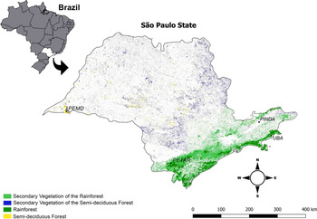
Sampling for euglossines was conducted at four Atlantic forest remnants in the state of São Paulo, Brazil (Fig. 1; Supplementary material, Table S1). Selected sampling areas were located 61–750 km apart. Specimens of El. nigrita were collected from each location. We chose this species because it was present in high densities in all sampling areas; other species could not be used to improve our analysis because they were present at only one or two of the sampling locations (see Machado et al. Reference Machado, Costa and Francoy2018 for more details concerning the Euglossini species composition in these locations).
Map showing the study areas with different phytophysiognomies in four remnants of Atlantic forest located in the state of São Paulo, southeast Brazil. PEMD, Parque Estadual Morro do Diabo; PETAR, Parque Estadual Turístico do Alto Ribeira; PINDA, Pindamonhangaba; UBA, Ubatuba.

We chose to consider two different physiognomies. For Atlantic rainforest, we collected bees from the state park, Parque Estadual Turístico do Alto Ribeira (24° 27′ 36″ S, 48° 36′ 0″ W), and from Ubatuba (22° 27′ 0″ S, 52° 10′ 0″ W). For Atlantic semi-deciduous forest, samples were collected from Pindamonhangaba (22º 55′ 50″ S, 45º 27′ 22″ W) and from the state park, Parque Estadual Morro do Diabo (22° 27′ 0″ S, 52° 10′ 0″ W). These regions differ in climate, in which a warm and wet climate without a dry season predominates throughout the Atlantic rainforest, and the Atlantic semi-deciduous forest is characterised by a seasonal climate with a relatively severe dry season (Morellato and Haddad Reference Morellato and Haddad2000; but see Machado et al. Reference Machado, Costa and Francoy2018 for more details concerning sampling areas).
Bees were collected from April 2014 to March 2015 in Ubatuba and Pindamonhangaba and from May 2014 to April 2015 in Parque Estadual Morro do Diabo and Parque Estadual Turístico do Alto Ribeira. The sampling method was based on Rebêlo and Garófalo (Reference Rebêlo and Garófalo1991), with minor modifications. In brief, we conducted the sampling on subsequent sunny days from 8:00 to 15:00 hours. We used baits that had scents used in similar studies and that showed good attractiveness to euglossine males (e.g., Uehara-Prado and Garófalo Reference Uehara-Prado and Garófalo2006; Rocha-Filho and Garófalo Reference Rocha-Filho and Garófalo2013, Reference Rocha-Filho and Garófalo2014; only males are attracted to scent baits, which is the reason why we chose to work with them). The baits were prepared from cotton wool wrapped in gauze and tied with a string; they were fixed to tree branches at the height of one metre above the ground and a distance of five metres apart. Bees were actively collected with entomological nets. All individuals were killed in 96% ethanol and preserved in this solution for subsequent molecular analysis. All specimens were stored in the laboratory, Laboratório de Genética e Conservação de Abelhas, Escola de Artes, Ciências e Humanidades, Universidade de São Paulo (São Paulo, São Paulo, Brazil), at –20 °C. For details concerning the sampling sites and methods, see Machado et al. (Reference Machado, Costa and Francoy2018).
The abundance data were derived from Machado et al. (Reference Machado, Costa and Francoy2018), but local abundances were also calculated in the present study (Supplementary material, Table S2). Relative abundances were calculated as the proportion of a species abundance versus the total euglossine abundance collected at that particular location.
DNA extraction
Total DNA was extracted from a hind leg of each of 126 males of El. nigrita using the Chelex DNA extraction method described by Walsh et al. (Reference Walsh, Metzger and Higuchi1991), with slight modifications. For DNA extraction, the leg was added to a solution of 100-µL Chelex (5% solution in water) with 5 µL of proteinase K (10 mg/mL; Merck KGaA, Darmstadt, Germany). This solution was incubated under the following conditions: 1 hour at 55 °C, followed by 15 minutes at 94 °C, and 1 minute at 37 °C. The DNA extractions were stored in microcentrifuge tubes and frozen at –20 °C for later analysis.
Microsatellite (simple sequence repeat) analysis
For genotyping, we used five microsatellite loci of El. nigrita (Eln 1, Eln 12a, Eln 12b, Eln 13, and Eln 2J) from Souza et al. (Reference Souza, Cervini, Del Lama and Paxton2007). Simple sequence repeat analyses were carried out according to the M13-tailing polymerase chain reaction technique (Schuelke Reference Schuelke2000) with a modified tail and M13-universal primer (M13-tail 5′-TTT CCC AGT CAC GAC GTT-3′, M13-universal primer 5′-AG GGT TTT CCC AGT CAC GAC GTT-3′). The M13-universal primer was used and labelled with one of three different fluorescent dyes: 6-FAN, NED, and HEX (Applied Biosystems, Thermo Fisher Scientific, Foster City, California, United States of America).
The polymerase chain reaction was performed according to Schuelke (Reference Schuelke2000), with slight modifications. Polymerase chain reaction was prepared by adding 1 µL of total extracted DNA, 0.5 µL of the forward primer with M13-tail (10 µM), 1 µL of the reverse primer (10 µM), 1 µL of M13-universal primer (10 µM) labelled with a fluorescent dye, and 5 µL Promega Master Mix 2.5
 $$ \times $$
in a total volume of 10 µL in nuclease-free water. The amplification of DNA was performed under the following conditions: an initial denaturing step of 2 minutes at 94 °C was followed by 35 cycles of 30 seconds at 94 °C, an annealing step of 20 seconds at 58 °C, and an extension step of 1 minute at 72 °C. This initial polymerase chain reaction protocol was followed by another for annealing the M13 primers under the following conditions: 15 cycles of 30 seconds at 94 °C, 30 seconds at 53 °C, and 1 minute at 72 °C, with a final elongation period at 72 °C for 10 minutes. Multiple, non-overlapping polymerase chain reaction fragments were pooled and diluted 1:30 with nuclease-free water. One microlitre of the diluted polymerase chain reaction product was added to 9 μL mix with highly deionised (Hi–Di) formamide (Applied Biosystems) and GenScan-500 ROX Size Standard (Applied Biosystems). Analyses of microsatellite fragment size were done on an ABI 3730 XL DNA Analyzer (Applied Biosystems) at the Centro de Recursos Biológicos e Biologia Genômica, Jaboticabal (CREBIO, Universidade Estadual Paulista; Jaboticabal, São Paulo, Brazil). Alleles were scored automatically, and the results were corrected manually in case of errors in the automatic scoring. Peaks were called and binned with the microsatellite plugin of Geneious, version 7.1.3 (Kearse et al. Reference Kearse, Moir, Wilson, Stones-Havas, Cheung and Sturrock2012). We used POWSIM, version 4.1 (Ryman and Palm Reference Ryman and Palm2006) to assess the power of our microsatellite data set. We set the effective population size (Ne) to 500 and repeated the entire process of drift, sampling, and statistical testing 10 000 times. In addition, we tested for linkage disequilibrium among loci over all sampled populations using GENEPOP, version 4.7 (Raymond and Rousset Reference Raymond and Rousset1995; Rousset Reference Rousset2008).
Genetic diversity by simple sequence repeats
Genetic diversity was measured by the sample size–corrected allelic richness and by Nei’s unbiased expected heterozygosity per population (Nei Reference Nei1977). Expected heterozygosity was calculated from haploid data as an estimate of this parameter for a diploid population (e.g., females). These parameters were calculated using GenAlEx, version 6.5 (Peakall and Smouse Reference Peakall and Smouse2006, Reference Peakall and Smouse2012) and the diveRsity package in R (Keenan et al. Reference Keenan, McGinnity, Cross, Crozier and Prodöhl2013), respectively. To test if habitat and relative abundance influenced genetic diversity (here, it refers only to allelic richness values) in each locality, linear mixed models were performed for allelic richness with the lmer function in the R package, lme4, version 1.1–10 (Bates et al. Reference Bates, Maechler, Bolker and Walker2015), as described in Soro et al. (Reference Soro, Quezada-Euan, Theodorou, Moritz and Paxton2017) and Maebe et al. (Reference Maebe, Karise, Meeus, Mänd and Smagghe2019a, Reference Maebe, Karise, Meeus, Mänd and Smagghe2019b). The model included habitat (considering the two physiognomies, rainforest and semi-deciduous forest), relative abundance as the fixed factors, and microsatellite loci as a random factor (Soro et al. Reference Soro, Quezada-Euan, Theodorou, Moritz and Paxton2017; Barton Reference Barton2020). The best model that fits our data was selected based on the Akaike’s information criterion by using the “dredge” command within the MUMIn package (Barton Reference Barton2020; Maebe et al. Reference Maebe, Karise, Meeus, Mänd and Smagghe2019a and references therein). The main effect of the factor of interest was analysed for each selected linear mixed model by performing likelihood ratio tests comparing the models with factors to a “null” model without these factors (Soro et al. Reference Soro, Quezada-Euan, Theodorou, Moritz and Paxton2017; Maebe et al. Reference Maebe, Karise, Meeus, Mänd and Smagghe2019a and references therein). We estimated the variance of each of habitat and abundance alone versus the variance for microsatellite loci variability, as the marginal and conditional coefficient of determination, respectively (Nakagawa and Schielzeth Reference Nakagawa and Schielzeth2013; Soro et al. Reference Soro, Quezada-Euan, Theodorou, Moritz and Paxton2017). Tukey honestly significant difference post hoc comparisons were also made using the R package multcomp (Hothorn et al. Reference Hothorn, Bretz and Westfall2008) to find differences in genetic diversity due to habitat or relative abundance alone (described in Soro et al. Reference Soro, Quezada-Euan, Theodorou, Moritz and Paxton2017; Maebe et al. Reference Maebe, Karise, Meeus, Mänd and Smagghe2019a and references therein). All of the tests in our study were performed using the statistical package R, version 3.6.1 (R Core Team 2019), following the guidelines of a free available tutorial (https://popgen.nescent.org/LMM-Genetic-Diversity.html). The R code can be found in Supplementary materials. Any P-values less than 0.05 were considered significant.
Genetic differentiation by simple sequence repeats
Genetic differentiation was estimated by Phi PT for haploid data, using GenAlEx. We also calculated F ST (calculated in GenAlEx by Nei’s formula for G ST (Nei Reference Nei1977), a multiallelic expansion of Wright’s F ST (Meirmans and Hedrick Reference Meirmans and Hedrick2011)) from a diploidised data set, as described in Soro et al. (Reference Soro, Quezada-Euan, Theodorou, Moritz and Paxton2017). Significance for estimators of genetic differentiation was derived by permuting 999 times across samples. In addition, principal coordinates analysis was performed using a standardised genetic distance matrix to check for population substructuring. The population structuring was also investigated by performing a Bayesian clustering algorithm imbedded in Structure, version 2.3.4 (Pritchard et al. Reference Pritchard, Stephens and Donnelly2000). The number of best-fitting populations (K) was explored using the admixture model, which was set with a configuration of 100 000 cycles and 500 000 repetitions (as described by Toledo et al. Reference Toledo, Junqueira, Augusto and Brito2017) of the Markov chain Monte Carlo. K-values ranged from 1 to 6 and were repeated 10 times. The best K-value was determined by the Evanno method imbedded in the programme, Structure Harvester, version 0.6.94 (Earl and vonHoldt Reference Earl and von Holdt2012).
We also computed analysis of molecular variance for three hierarchical levels: (1) within sampling sites, (2) among sampling sites, and (3) among regions (considering each physiognomy as a region). To test for isolation by distance, we performed Mantel tests, as implemented in GenAlEx. The genetic differentiation was also examined with the assignment test in GenAlEx in order to determine the percentage of individuals correctly assigned to their original population. The geographic-distance matrices were calculated from the minimum distance of different groups among the sampling sites (Supplementary material, Table S1). Genetic distances were generated using pairwise F ST values, as described in Zayed and Packer (Reference Zayed and Packer2007) and Toledo et al. (Reference Toledo, Junqueira, Augusto and Brito2017). In all analyses, only P-values < 0.05 were considered significant.
Mitochondrial DNA analysis
The primers mtD26 (TAT GTA CTA CCA TGA GGA CAA ATA TC) and mtD28 (ATT ACA CCT CCT AAT TTA TTA GGA AT) of the mitochondrial cytochrome b (Cyt B) gene described by Crozier et al. (Reference Crozier, Koulianos and Crozier1991) were used in polymerase chain reactions, according to López-Uribe and Del Lama (Reference López-Uribe and Del Lama2007), with slight modifications. The polymerase chain reaction was prepared by adding 2.5 µL of total extracted DNA, 2.5 µL (10 µM) of each specific primer, and 25 µL Promega Master Mix 2.5
 $$ \times $$
in a total volume of 50 µL in nuclease-free water. The amplification of DNA was performed under the following conditions: an initial denaturation step at 94 °C for 5 minutes, followed by 37 cycles of 1 minute at 94 °C, an annealing step of 1 minute at 42 °C, and an extension step of 3 minutes at 64 °C, as well as a final extension step of 10 minutes at 64 °C. The amplification products were visualised on 1% agarose gels. The polymerase chain reaction product was purified with Wizard SV Gel and PCR Clean-Up System (Promega Corporate, Madison, Wisconsin, United States of America) and subsequently subjected to sequencing (CREBIO – Centro de Recursos Biológicos e Biologia Genômica, UNESP Jaboticabal). The sequences were aligned and edited using Geneious, version 7.1.3 (Kearse et al. Reference Kearse, Moir, Wilson, Stones-Havas, Cheung and Sturrock2012). In order to compare the differences among the obtained sequences, we also used a Cyt B mitochondrial sequence from a specimen from Panama (accession number AY916095.1).
Results
Microsatellite (simple sequence repeat) analysis
All microsatellite loci were amplified and scored reliably for 116 specimens out of 126 analysed individuals (Supplementary material, Table S2). The results of our POWSIM analyses showed that the markers are powerful enough to detect population differentiation correctly but a relatively small number of loci. A power of 0.80 or greater has been suggested as the threshold for providing adequate statistical power (Cohen Reference Cohen1988); our analysis indicated that our data set has a power of 0.95 to detect genetic differentiation (values provided from chi-squared test). Also, linkage disequilibrium was not detected for pairs of loci among the El. nigrita populations from our sampling areas; similar results were found in other studies (Souza et al. Reference Souza, Cervini, Del Lama and Paxton2007, Reference Souza, Del Lama, Cervini, Mortari, Eltz and Zimmermann2010; Zimmermann et al. Reference Zimmermann, Schorkopf, Moritz, Pemberton, Quezada-Euan and Eltz2011; Rocha-Filho et al. Reference Rocha-Filho, Cerântola, Garófalo, Imperatriz Fonseca and Del Lama2013).
Genetic diversity by simple sequence repeats
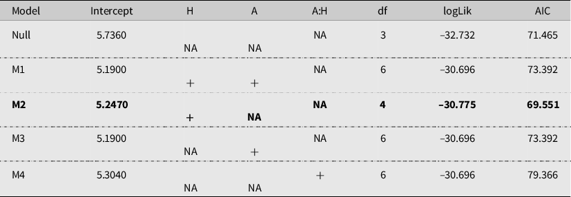
Overall, for populations, mean expected heterozygosity was 0.731, with individual population values ranging from 0.651 to 0.766 (Table 1). Allelic richness ranged from 5 to 8.2, with a mean richness of 6.3 (Table 1), reflecting a considerable variability in genetic diversity, which we account for in subsequent analyses by fitting linear mixed models. When comparing the Akaike’s information criterion scores of the different linear mixed models, the best model explaining the observed patterns of genetic diversity (here, it refers to allelic richness values) was the model with “habitat” (here, it refers to phytophysiognomies) as the only fixed factor (Table 2). The importance of the factor “habitat” for genetic diversity was shown by comparing the models with and without “habitat” as a fixed factor (likelihood ratio test: χ 2 = 3.914, df = 1, P = 0.04). Furthermore, the addition of relative abundance as an extra fixed factor had no significant impact on the model, as became apparent after comparing the models with both “habitat” and “abundance” as fixed factors to the models without these factors as additional fixed factors (likelihood ratio test: χ 2 = 4.073, df = 3, P = 0.254). The variance accounted for by habitat alone (marginal R 2) was 15.8%, whereas the variance accounted for by marker variability (conditional R 2) was 36.6% (Nakagawa and Schielzeth Reference Nakagawa and Schielzeth2013). Post hoc tests indicated significant differences in genetic diversity levels only between the habitat types (z = 2.115, P = 0.035) – that is, rainforest and semi-deciduous forest, the latter being the most diverse.
Genetic diversity of Eulaema nigrita from four sampling sites in the Atlantic forest. Allelic richness (AR) and expected heterozygosity (He) for overall populations.

SE, corresponding standard error; PEMD, Parque Estadual Morro do Diabo; PETAR, Parque Estadual Turístico do Alto Ribeira; PINDA, Pindamonhangaba; UBA, Ubatuba.
Selection of the best-fitting model explaining the genetic diversity pattern. The models included habitat (H) and/or relative abundance (A) as the fixed factors and microsatellite loci as a random factor. The best model fitting our data was selected based on the Akaike’s information criterion (AIC). (+) parameters included in the model, and NA, not included parameters. The selected best model is indicated in bold.

Genetic differentiation by simple sequence repeat
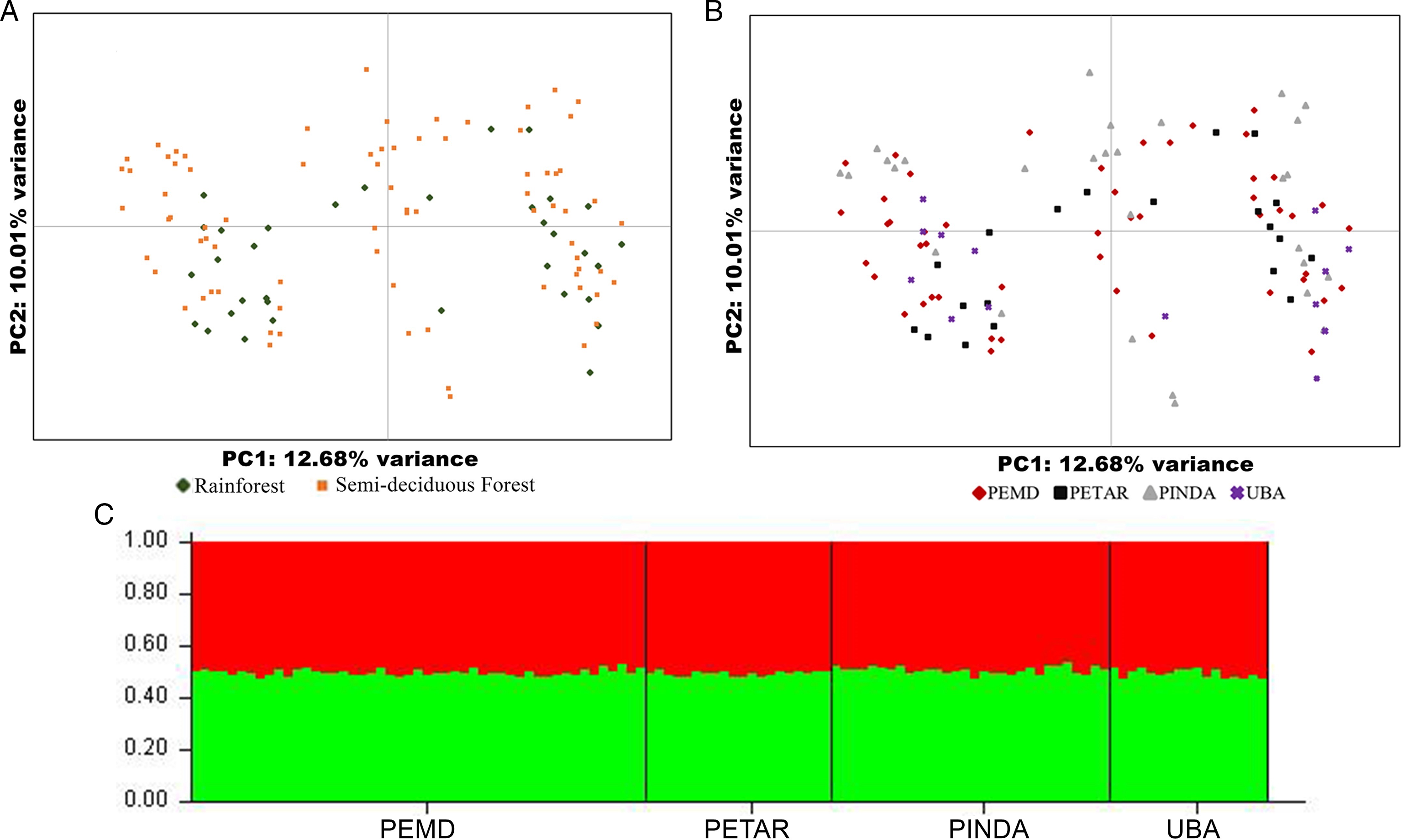
Global genetic differentiation was consistently low across estimators, although significantly different from zero (Phi PT = 0.071, P = 0.001; F ST = 0.087, P = 0.001). Estimates of pairwise F ST for sampling sites were low but significantly different from zero (Table 3), except between Parque Estadual Morro do Diabo and Parque Estadual Turístico do Alto Ribeira (F ST = 0.017, P values = 0.532). Similar results were observed for pairwise Phi PT comparisons (Supplementary material, Table S3). Hence, based on two first principal coordinates, the principal coordinates analysis plot did not form a cluster according to physiognomies (Fig. 2A). We observed a similar result for localities, which did not show a clear spatial pattern among populations (Fig. 2B). By applying the Evanno method embedded in Structure Harvester, we identified K = 2 as the most likely number of subgroups for the genotypes among all four study areas. However, we did not observe two distinct groups of genotypes (Fig. 2C). This indicates that the sampling sites are not structured and all individuals are from one unique population (Fig. 2C). Consistent with these results, analysis of molecular variance that considered habitat (physiognomies) showed that most of the molecular variance was within sampling sites (94%). Variance among sampling sites could be partitioned into 5% among sites within physiognomies and into 1% among physiognomies (rainforest and semi-deciduous forest; for more detail, see Supplementary material, Table S4). Supporting these conclusions, assignment tests showed that the chance of correct assignment of an individual to its respective population did not differ from an assignment by chance (50:50; Supplementary material, Table S5). We also detected no patterns of isolation by distance among the El. nigrita populations (Mantel R 2 = 0.025, P = 0.380).
Pairwise F ST values (below diagonal) and statistical significance (above diagonal) among populations of Eulaema nigrita.

PEMD, Parque Estadual Morro do Diabo; PETAR, Parque Estadual Turístico do Alto Ribeira; PINDA, Pindamonhangaba; UBA, Ubatuba.
α = 0.05. Significant F ST values are indicated in bold (below diagonal).
Patterns of geographical structure for Eulaema nigrita in remnants of Atlantic forest in the state of São Paulo, southeast Brazil. A, Principal coordinates analysis (PCoA) among individuals of Eulaema nigrita as compared to habitat based on a standardised genetic distance matrix obtained from microsatellite loci genotypic data; B, principal coordinates analysis (PCoA) among individuals of Eulaema nigrita compared to locations based on standardised genetic distance matrix obtained from microsatellite loci genotypic data; C, graphical representation of the genetic structure of the sampling areas. Each vertical line represents a specimen, and allele frequencies are coloured: red and green represent the two genotypic groups (K = 2). PEMD, Parque Estadual Morro do Diabo; PETAR, Parque Estadual Turístico do Alto Ribeira; PINDA, Pindamonhangaba; UBA, Ubatuba.

Mitochondrial DNA
Among the 126 samples, only 105 amplified the expected fragment from Cyt B, a mitochondrial gene. We amplified a 308-bp Cyt B gene fragment. The same Cyt B haplotype was observed in all forest remnants, even with a distance of up to 700 km separating samples that were farthest apart. Additionally, we found a difference of three base pairs (or 1.1%, because the sequence used for comparison is only 261 base pairs long) between our samples and a Panamanian specimen based on a mitochondrial sequence (accession number AY916095.1), indicating high similarity.
Discussion
Because El. nigrita is considered a good long-distance flyer (Janzen Reference Janzen1971), in the present study, we tested two hypotheses regarding genetic diversity and population structure: (1) that orchid bee local abundance and type of habitat determine population genetic diversity levels; and (2) that high genetic diversity and no population structure are expected for this species due to its high dispersal ability. By genotyping specimens from four locations – two from each of two different vegetation types – we found that habitat is associated with the genetic diversity of El. nigrita across our sampling areas. Although this analysis was based on a relatively limited number of loci, the results of our POWSIM analyses showed that this data set provides significant statistical power to detect genetic diversity and population differentiation among our sampled specimens. A limited number of loci has also been used to document population differentiation in Euglossini in other studies (Zimmermann et al. Reference Zimmermann, Schorkopf, Moritz, Pemberton, Quezada-Euan and Eltz2011; Freiria et al. Reference Freiria, Ruim, de Souza and Sofia2012; Soro et al. Reference Soro, Quezada-Euan, Theodorou, Moritz and Paxton2017), leading us to conclude that our analyses are robust and that our results reflect overall trends in genetic variation in our study species.
Nonetheless, when comparing the nuclear genetic diversity with relative abundance and type of habitat, we conclude that observed genetic diversity was not significantly correlated with local species abundance but that the type of habitat significantly influenced it. Indeed, the best linear mixed model explaining the genetic diversity patterns did not include relative abundance; habitat was the only significant factor. We found greater genetic diversity in semi-deciduous forest than in rainforest areas. These results did not support the idea that a large population for a certain species should have higher genetic diversity than a smaller population. Similarly, Maebe et al. (Reference Maebe, Karise, Meeus, Mänd and Smagghe2019a) found that the local abundance of bumblebee species was not directly determined by genetic variation. Our findings also agree with Silva and De Marco (Reference Silva and De Marco2014), who found no relation between the abundance of El. nigrita and landscape features. Rocha-Filho et al. (Reference Rocha-Filho, Cerântola, Garófalo, Imperatriz Fonseca and Del Lama2013) also found no evidence of correlation between numbers of males analysed and genetic diversity.
Although no correlation between genetic variation and abundance was found in the present study, we observed a significant correlation between genetic diversity and habitat. Both results can be attributed to spatiotemporal differences in resources or even in nesting resource availability (Zimmermann et al. Reference Zimmermann, Schorkopf, Moritz, Pemberton, Quezada-Euan and Eltz2011) because both can significantly affect the size of offspring broods. First, quantitative fluctuations in the composition of orchid bee populations across the landscape suggest that observed relative abundances also represent “snapshots” of the population’s dynamics, as stated by Zimmermann et al. (Reference Zimmermann, Schorkopf, Moritz, Pemberton, Quezada-Euan and Eltz2011). Second, the differences in forest cover across landscapes in a comparison of open and forest areas seem to have affected genetic diversity (for more details about the vegetation cover, see Costa et al. Reference Costa, Machado, Santiago, Dallacqua, Garófalo and Francoy2020). This agrees with studies on other euglossine species that found differences in genetic variation in different areas, in particular between mainland and islands (Rocha-Filho et al. Reference Rocha-Filho, Cerântola, Garófalo, Imperatriz Fonseca and Del Lama2013; Boff et al. Reference Boff, Soro, Paxton and Alves-dos-Santos2014; Soro et al. Reference Soro, Quezada-Euan, Theodorou, Moritz and Paxton2017) and for other bee groups (Ellis et al. Reference Ellis, Knight, Darvill and Goulson2006; Davis et al. Reference Davis, Murray, Fitzpatrick, Brown and Paxton2010; Soro et al. Reference Soro, Field, Bridge, Cardinal and Paxton2010; Lozier et al. Reference Lozier, Strange and Koch2013). Moreover, it has been reported that El. nigrita is most commonly encountered in open areas (Rebêlo and Garófalo Reference Rebêlo and Garófalo1997; Alvarenga et al. Reference Alvarenga, Freitas and Augusto2007) and is associated with disturbed and anthropic matrices (Morato Reference Morato1998; Peruquetti et al. Reference Peruquetti, Campos, Coelho, Abrantes and Lisboa1999; Tonhasca et al. Reference Tonhasca, Blackmer and Albuquerque2002). As expected, we found a significant effect of habitat on genetic diversity. Differences occurred based on forest cover and the number of anthropic areas, resulting in spatial differences in resources and, consequently, affecting genetic variation.
Concerning allelic richness and expected heterozygosity, we found high genetic diversity at all sites, which other studies had also found (Rocha Filho et al. Reference Rocha-Filho, Cerântola, Garófalo, Imperatriz Fonseca and Del Lama2013; Penha et al. Reference Penha, Gaglianone, Almeida, Boff and Sofia2015). Two plausible reasons for high genetic diversity in these populations are high gene flow and high effective population size. High gene flow is also evident, based on the weak structure among these populations. Even for males collected from locations that are as far as 750 km apart, we found a significant but extremely low population genetic structure. Our results and those of previous studies (Janzen Reference Janzen1971, Reference Janzen1981; Raw Reference Raw1989; Tonhasca et al. Reference Tonhasca, Albuquerque and Blackmer2003; Dick et al. Reference Dick, Roubik, Gruber and Bermingham2004; Sofia et al. Reference Sofia, Paula, Santos, Almeida and Sodré2005; Zimmermann et al. Reference Zimmermann, Schorkopf, Moritz, Pemberton, Quezada-Euan and Eltz2011; Rocha-Filho et al. Reference Rocha-Filho, Cerântola, Garófalo, Imperatriz Fonseca and Del Lama2013) support the hypothesis that males of some Euglossini species can cover distances that are greater than the shortest distances between our locations. Studies indicate, based on morphological characters, a lack of differences among populations of El. nigrita (Pinto et al. Reference Pinto, Silva, Rodrigues and De Marco2015; Costa et al. Reference Costa, Machado, Santiago, Dallacqua, Garófalo and Francoy2020) and across seasons (Silva et al. Reference Silva, Lomônaco, Augusto and Kerr2009). Eulaema nigrita is a high-dispersal species (Raw Reference Raw1989), which is an important factor that can explain the low F ST value found in our results. When we consider a theoretical scale (Wright Reference Wright1978) for parameters used to measure the degree of genetic differentiation, such as F ST or Phi PT, we found a very low to modest level of genetic differentiation between population pairs, similar to the global estimates of F ST and Phi PT, which were both very low. These observations were also supported by mitochondrial DNA data, with no differentiation because we found only one haplotype among our sampling sites. Our assignment test also indicated that the chance of an individual being correctly assigned to its original population was similar to the values of purely random assignment (50%). Rocha-Filho et al. (Reference Rocha-Filho, Cerântola, Garófalo, Imperatriz Fonseca and Del Lama2013) found a similar result for Eulaema species.
In addition, our findings agree with those of previous studies that orchid bees have a weak population structure (Dick et al. Reference Dick, Roubik, Gruber and Bermingham2004; Zimmermann et al. Reference Zimmermann, Schorkopf, Moritz, Pemberton, Quezada-Euan and Eltz2011; Rocha-Filho et al. Reference Rocha-Filho, Cerântola, Garófalo, Imperatriz Fonseca and Del Lama2013). Dick et al. (Reference Dick, Roubik, Gruber and Bermingham2004) also observed identical mitochondrial DNA haplotypes in cross-Andean populations of El. nigrita. Based on molecular data, these authors showed that the dispersal abilities of some orchid bee species present a positive correlation with body size (Dick et al. Reference Dick, Roubik, Gruber and Bermingham2004); larger body size may provide a means for long-distance dispersal and founder events. The low divergence and the finding of only one haplotype through the different Atlantic forest fragments provide additional support for the morphological identification of El. nigrita, as found by Costa et al. (Reference Costa, Machado, Santiago, Dallacqua, Garófalo and Francoy2020). Although long-distance dispersal appears to be characteristic of orchid bees (Janzen Reference Janzen1971), an alternative explanation for the weak population structure may be that there has not been sufficient time for isolation to cause genetic effects. During the last four decades, alterations in the sampling areas increased and include marked changes in forest cover between 1960 and 2006 due to agriculture intensification in many areas (Calaboni et al. Reference Calaboni, Tambosi, Igari, Farinaci, Metzger and Uriarte2018). However, as shown by Pinto et al. (Reference Pinto, Silva, Rodrigues and De Marco2015), there is no evidence of habitat loss affecting El. nigrita. The two factors – a strong capacity for dispersion and insufficient time for isolation – can directly contribute to homogeneity among populations, even over large distances. Based on our data and also on previous data collected by our group (Grassi-Sella et al. Reference Grassi-Sella, Garófalo and Francoy2018; Machado et al. Reference Machado, Costa and Francoy2018; Costa et al. Reference Costa, Machado, Santiago, Dallacqua, Garófalo and Francoy2020), it appears that forest fragmentation does not pose a threat to Euglossini bees, because no population structure has been found. Because the Atlantic rainforest is incredibly reduced, if restoration is not possible (the ideal option), the preservation of different fragments of similar physiognomies may be enough, at least for long-distance flyers. However, more studies are needed for bees that are not as good at dispersing as Euglossini bees are.
Acknowledgements
The authors are grateful to Agência Paulista de Tecnologia dos Agronegócios (APTA-SAA, São Paulo, Brazil), in particular, Dr. Érica Weinstein Teixeira, for support and infrastructure for our sampling in Ubatuba and Pindamonhangaba. The authors thank the Centro de Recursos Biológicos e Biologia Genômica – UNESP Jaboticabal (CREBIO) for DNA sequencing and genotyping. They also thank IBAMA (Brazilian Institute of Environment and Renewable Natural Resources)/ICMBio-Sisbio (Institute Chico Mendes – MMA) for permission to collect the bees. Dr. David de Jong kindly helped the authors to improve the English of our manuscript.
This study was supported by FAPESP (Fundação de Amparo à Pesquisa do Estado de São Paulo – Processes 2011/07857–9 to TMF and 2013/02158–0 to CPC) and CAPES (Coordenação de Aperfeiçoamento de Pessoal de Nível Superior – Brasil – Finance Code 001 to CASM). Contributions: CPC was involved in data acquisition, data analysis and helped write the paper; TMF helped plan the work and helped write the paper; and CASM participated in data acquisition and helped review the manuscript. Conflicts of interest: The authors declare no conflict of interest.
Data availability
Raw microsatellite data are available from the Dryad Digital Repository (https://doi.org/10.6086/D11M3Q). Mitochondrial DNA data generated during this study are available in the GenBank repository (accession numbers MN829949-MN830053). Restrictions apply to the availability of these data; they are not publicly available until article publication.
Supplementary material
To view supplementary material for this article, please visit https://doi.org/10.4039/tce.2021.19.