1 Introduction
Turbulence in the atmosphere and oceans is intermittent in time and inhomogeneous in space (Baker & Gibson Reference Baker and Gibson1987). Parameterisation of small-scale turbulent quantities in global circulation models is thus both very challenging and very important (Ivey, Winters & Koseff Reference Ivey, Winters and Koseff2008). One conventional avenue of research has been the consideration of flow instabilities, as they naturally are mechanisms by which disordered motions can arise from a laminar flow. A very commonly considered instability-mediated route to turbulence is via the so-called Kelvin–Helmholtz instability (KHI) (or, perhaps more appropriately, ‘stratified Rayleigh instability’). This normal-mode instability develops in stably stratified shear flows with inflectional background profiles of velocity and density (or, equivalently, buoyancy) when the destabilising effect of the shear is sufficiently strong to overcome the stabilising effect of the stratification for infinitesimal perturbations. The finite amplitude manifestation of the KHI takes the form of elliptical vortices or ‘billows’, which have been observed in multiple oceanic circumstances (Smyth & Moum Reference Smyth and Moum2012), including in the thermocline (Woods Reference Woods1968), the abyssal ocean (van Haren & Gostiaux Reference van Haren and Gostiaux2010) and above continental shelves (Moum et al. Reference Moum, Farmer, Smyth, Armi and Vagle2003). Many laboratory experiments and numerical simulations have been performed to investigate the initiation, development and breakdown of KHIs (Thorpe Reference Thorpe1973; Klaassen & Peltier Reference Klaassen and Peltier1985; Fernando Reference Fernando1991; Peltier & Caulfield Reference Peltier and Caulfield2003), which are known to be prone, particularly for sufficiently large Reynolds numbers, to a large ‘zoo’ of secondary instabilities (Mashayek & Peltier Reference Mashayek and Peltier2012a ).
From consideration of the Taylor–Goldstein equation (Goldstein Reference Goldstein1931; Taylor Reference Taylor1931), it is possible to derive the influential ‘Miles–Howard’ criterion (Howard Reference Howard1961; Miles Reference Miles1961), which states that a sufficient condition for linear stability of an inviscid incompressible stably stratified shear flow defined by a (laminar) steady parallel velocity profile
 $\bar{U}(z)$
and buoyancy frequency
 $N(z)=\sqrt{-g/\bar{\unicode[STIX]{x1D70C}}\,\text{d}\bar{\unicode[STIX]{x1D70C}}/\text{d}z}$
(where
 $\bar{\unicode[STIX]{x1D70C}}(z)$
is the background density distribution and
 $g$
is the acceleration due to gravity) is that the gradient Richardson number
 $Ri_{g}(z)\geqslant 1/4$
everywhere in the flow, where
 $$\begin{eqnarray}Ri_{g}(z)=\frac{N^{2}}{(\text{d}\bar{U}/\text{d}z)^{2}}.\end{eqnarray}$$
Significantly, Thorpe & Liu (Reference Thorpe and Liu2009) applied this criterion to develop the concept of ‘marginal instability’ to interpret and predict the existence of a range of naturally occurring stably stratified turbulent flows. In this particular context, the marginal instability of a flow is quantified by a parameter
 $\unicode[STIX]{x1D6F7}$
, which is the fractional change in flow speed required to ensure linear stability of the flow. By applying the critical value of
 $Ri_{c}=1/4$
to this idea,
 $\unicode[STIX]{x1D6F7}$
satisfies
 $$\begin{eqnarray}(1+\unicode[STIX]{x1D6F7})^{2}=4Ri,\end{eqnarray}$$
where
 $Ri$
is some characteristic (typically the minimum,
 $Ri_{m}$
) value of the gradient Richardson number
 $Ri_{g}$
. A flow is then said to be marginally unstable if it is in a linearly unstable state (so
 $Ri<1/4$
and hence
 $\unicode[STIX]{x1D6F7}<0$
) and the fractional change is small compared with unity (
 $|\unicode[STIX]{x1D6F7}|\ll 1$
).
It is important to distinguish between this particular meaning of ‘marginal stability’, based around the concept of linear normal-mode instabilities growing and ultimately triggering turbulence, and an alternative meaning based around the concept of inherently nonlinear processes maintaining turbulence for sufficiently low values of a Richardson number defined in terms of the mean profiles of velocity and density. Smyth & Moum (Reference Smyth and Moum2013) discussed application of the ‘linear’ marginal instability concept as proposed by Thorpe & Liu (Reference Thorpe and Liu2009) to turbulent flows, but also provided an alternative to the latter’s linear stability arguments, to explain observations of deep cycle turbulence with a Richardson number close to 1/4. They used the results of Rohr et al. (Reference Rohr, Itsweire, Helland and Atta1988), which showed growth and decay of stratified turbulence below and above
 $Ri=1/4$
respectively, effectively thus applying the ‘nonlinear’ marginal stability concept to the maintenance of turbulence. In a distinct (although somewhat related) approach, Thorpe, Smyth & Li (Reference Thorpe, Smyth and Li2013) added an eddy viscosity and eddy diffusivity to the Taylor–Goldstein equation to modify the critical Richardson number in the Miles–Howard criterion. These added diffusive effects modelled a key property of a weakly turbulent background flow, but this approach was still based around appealing to linear instability processes with (an appropriate)
 $Ri$
close to the Miles–Howard criterion as the mechanism by which perturbations can grow to sufficiently large amplitude to maintain the turbulence. Indeed, since any small perturbation will be modified by small-scale turbulence in such a flow, the validity of performing linear stability analysis in this regime is at least formally questionable, especially if the predicted growth rate is small. Despite this, they claimed that application of the concept of marginal instability to such flows may explain the behaviour of shear layers after KHI breakdown.
For inviscid flows susceptible to KHI, as
 $Ri_{m}$
approaches
 $1/4$
from below, the exponential growth rate of the linear instabilities is predicted to drop to zero (Hazel Reference Hazel1972). However, this prediction does not in itself preclude the possibility that the finite amplitude ‘billow’ can still have significant amplitude for flows with such ‘marginal’ Richardson numbers, particularly in light of the results of Kaminski, Caulfield & Taylor (Reference Kaminski, Caulfield and Taylor2017). Using a direct-adjoint-looping method, they demonstrated that billow-like structures with non-trivial amplitude can still be triggered by ‘linear optimal’ perturbations of small initial perturbation energy (i.e. non-normal perturbations with a structure that exhibits maximum transient perturbation energy growth over a finite time interval) in flows where
 $Ri_{g}>1/4$
everywhere initially. However, the classical Miles–Howard criterion cited in the linear marginal stability arguments does not apply to these non-normal perturbations, and so we focus our study on normal-mode perturbations. Despite all of these caveats, it is still at least conceivable that a billow could reach large amplitude at very late times for a marginally unstable flow.
Our principal aim here is to investigate whether marginal instability, in the above-discussed sense of being based around linear stability arguments for the triggering of, rather than the maintenance of, pre-existing turbulence, is useful in describing transitional flows, with finite yet large Reynolds number
 $U_{0}d_{0}/\unicode[STIX]{x1D708}$
, where
 $\unicode[STIX]{x1D708}$
is the kinematic viscosity,
 $d_{0}$
is the shear-layer half-depth and
 $U_{0}$
is half of the velocity difference across the shear layer. For simplicity, we restrict attention to flows with
 $Pr=\unicode[STIX]{x1D708}/\unicode[STIX]{x1D705}=1$
, where
 $\unicode[STIX]{x1D705}$
is the density diffusivity. We are particularly focused on determining whether saturated billows of non-trivial amplitude can develop in such flows perturbed by normal-mode perturbations associated with the classical KHI in flows where
 $Ri_{m}\simeq 1/4$
. Since the growth rate of such instabilities gets very small as
 $Ri_{m}$
approaches
 $1/4$
from below, we consider three classes of flows: class ‘D’, where the background distributions of velocity and density diffuse naturally (thus modifying and increasing
 $Ri_{g}(z)$
with time); class ‘S’, with imposed body forces designed to maintain ‘steady’ background distributions (and hence
 $Ri_{g}$
remains close to constant in time); and class ‘A’, where
 $U_{0}$
increases exponentially with time so that
 $Ri_{m}$
can decrease through
 $1/4$
. In particular, this last class allows us to test the viability of ‘marginally unstable’ flows to develop perturbation billows of significant amplitude. We are principally interested in the viability of the marginal instability/stability concepts as mechanisms to drive or trigger self-limiting turbulent flows, and so we are only interested in identifying the maximum amplitude (and the time at which this occurs) of the billows. Therefore, we restrict our numerical calculations to two dimensions, precluding any consideration of subsequent secondary instabilities, or indeed the ensuing turbulent breakdown and associated irreversible mixing. (As we discuss below, our observed initial maximum amplitudes of inherently two-dimensional KHI billows are consistent with the three-dimensional simulation results of Mashayek, Caulfield & Peltier (Reference Mashayek, Caulfield and Peltier2013), giving us confidence that our two-dimensional calculations yield useful estimates for the amount of energy that can be transiently stored in a billow, and thus be ultimately available to drive turbulent motions.) The rest of the paper is organised as follows. In § 2, we describe our numerical model, the choice of domain and initial conditions. In § 3, we describe the particular characteristics of the three qualitatively different classes of flows we consider, and analyse the results of the simulations of each of these three different classes, identifying the key parameters controlling perturbation growth. Finally, we discuss the implications of our findings in § 4, particularly regarding the viability of the linear marginal (in)stability concepts as predictors of energetic turbulence and mixing in stratified shear flows.
2 Simulation set-up
We are interested in flows susceptible to primary instabilities of Kelvin–Helmholtz type, and so we consider dimensional (marked with an asterisk) background velocity
 $\bar{U}^{\ast }(z^{\ast })$
and buoyancy
 $\bar{B}^{\ast }(z^{\ast })=g^{\ast }(\unicode[STIX]{x1D70C}_{a}^{\ast }-\bar{\unicode[STIX]{x1D70C}}^{\ast })/\unicode[STIX]{x1D70C}_{a}^{\ast }$
distributions,
 $$\begin{eqnarray}\bar{U}^{\ast }(z^{\ast })=U_{0}^{\ast }\tanh (z^{\ast }/d_{0}),\quad \bar{B}^{\ast }(z^{\ast })=(g^{\ast }\unicode[STIX]{x1D70C}_{0}^{\ast }/\unicode[STIX]{x1D70C}_{a}^{\ast })\tanh (z^{\ast }/d_{0}^{\ast })=B_{0}^{\ast }\tanh (z^{\ast }/d_{0}^{\ast }),\end{eqnarray}$$
where
 $g^{\ast }$
is the acceleration due to gravity,
 $\unicode[STIX]{x1D70C}_{a}^{\ast }$
is a reference density, and the Boussinesq approximation applies, so that
 $\unicode[STIX]{x1D70C}_{0}^{\ast }\ll \unicode[STIX]{x1D70C}_{a}^{\ast }$
. We perform two-dimensional direct numerical simulations using the Diablo software (Taylor Reference Taylor2008), which implements a combination of explicit third-order Runge–Kutta and implicit Crank–Nicholson schemes. The code solves the two-dimensional Boussinesq equations for the non-dimensional velocity, buoyancy and pressure fields
 $\boldsymbol{u}=(u,w)$
,
 $b$
and
 $p$
,
 $$\begin{eqnarray}\displaystyle \unicode[STIX]{x1D735}\boldsymbol{\cdot }\boldsymbol{u} & = & \displaystyle 0,\end{eqnarray}$$
 $$\begin{eqnarray}\displaystyle \frac{\unicode[STIX]{x2202}\boldsymbol{u}}{\unicode[STIX]{x2202}t}+\boldsymbol{u}\boldsymbol{\cdot }\unicode[STIX]{x1D735}\boldsymbol{u} & = & \displaystyle -\unicode[STIX]{x1D735}p+\frac{1}{Re}\unicode[STIX]{x1D6FB}^{2}\boldsymbol{u}+Ri_{0}\,b\,\hat{\boldsymbol{z}},\end{eqnarray}$$
 $$\begin{eqnarray}\displaystyle \frac{\unicode[STIX]{x2202}b}{\unicode[STIX]{x2202}t}+\boldsymbol{u}\boldsymbol{\cdot }\unicode[STIX]{x1D735}b & = & \displaystyle \frac{1}{RePr}\unicode[STIX]{x1D6FB}^{2}b.\end{eqnarray}$$
 $\boldsymbol{u}=\boldsymbol{u}^{\ast }/U_{0}^{\ast }$
,
 $b=b^{\ast }/B_{0}^{\ast }$
,
 $\boldsymbol{x}=\boldsymbol{x}^{\ast }/d_{0}^{\ast }$
and
 $t=t^{\ast }/(d_{0}^{\ast }/U_{0}^{\ast })$
. The key parameters are the Reynolds number
 $Re=U_{0}^{\ast }d_{0}^{\ast }/\unicode[STIX]{x1D708}^{\ast }$
, the Prandtl number
 $Pr=\unicode[STIX]{x1D708}^{\ast }/\unicode[STIX]{x1D705}^{\ast }$
(here,
 $Pr=1$
) and the bulk Richardson number
 $Ri_{0}=B_{0}^{\ast }d_{0}^{\ast }/{U_{0}^{\ast }}^{2}$
.
The computational domain is 20 non-dimensional units in the vertical (
 $z$
) direction, and free-slip no-flux boundary conditions are imposed at
 $z=\pm 10$
. This prevents boundary effects from interfering with the shear layer in the centre of the domain. Periodicity is imposed in the streamwise (
 $x$
) direction, and we choose the length of the domain to be the wavelength of the most unstable normal mode for each simulation. The initial non-dimensional background profiles are hence
 $U(z)=B(z)=\tanh (z)$
, which ensures that the gradient Richardson number is
 $$\begin{eqnarray}Ri_{g}(z)=Ri_{0}\frac{\text{d}B/\text{d}z}{(\text{d}U/\text{d}z)^{2}}=Ri_{0}\cosh ^{2}z\rightarrow Ri_{m}=Ri_{g}(0)=Ri_{0},\end{eqnarray}$$
where
 $Ri_{m}$
is the minimum, occurring at the midpoint of the shear layer
 $z=0$
. These background profiles are perturbed by the fastest growing normal-mode perturbations
 $\boldsymbol{u}^{\prime }$
and
 $b^{\prime }$
, giving the following initial conditions:
 $$\begin{eqnarray}\boldsymbol{u}|_{t=0}=U(z)\hat{\boldsymbol{x}}+\unicode[STIX]{x1D716}\boldsymbol{u}^{\prime },\quad b|_{t=0}=B(z)+\unicode[STIX]{x1D716}b^{\prime }.\end{eqnarray}$$
We calculate the normal modes using a matrix method code originally developed by Smyth & Peltier (Reference Smyth and Peltier1990), which implements a finite
 $Re/Pr$
generalisation of the Taylor–Goldstein equation (or, equivalently, a stratified generalisation of the Orr–Sommerfeld equation). The amplitude of the normal-mode perturbation is chosen such that an appropriate measure of the initial perturbation ‘energy’, defined in Kaminski, Caulfield & Taylor (Reference Kaminski, Caulfield and Taylor2014) as
 $$\begin{eqnarray}E=\frac{1}{2}\langle \boldsymbol{u}^{\prime },\boldsymbol{u}^{\prime }\rangle +\frac{Ri_{0}}{2}\langle b^{\prime },b^{\prime }\rangle =K+P,\end{eqnarray}$$
is equal to a prescribed value
 $E_{0}$
. (As our background buoyancy distribution has non-uniform gradient, this does not correspond precisely to the sum of the perturbation kinetic energy and the perturbation potential energy, but we use this measure for computational convenience and consistency with the previous study of Kaminski et al. (Reference Kaminski, Caulfield and Taylor2014).) We use the inner product
 $\langle \boldsymbol{u},\boldsymbol{v}\rangle =1/A\int _{A}\boldsymbol{u}\boldsymbol{\cdot }\boldsymbol{v}\,\text{d}x\,\text{d}z$
, where
 $A$
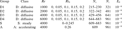
is the area of the domain. Table 1 lists the range of parameters used.
The parameters for the numerical simulations. The numbers of grid points in each direction are
 $N_{x}$
and
 $N_{z}$
, which are varied with
 $Re$
and
 $Ri_{0}$
to ensure accurate simulation of the flow.

By taking
 $\boldsymbol{u}^{\prime }$
and
 $b^{\prime }$
to be the perturbations to the initial background hyperbolic tangent profiles, we can measure the perturbation energy defined in (2.5) throughout the development of the shear layer. At early times, the perturbation energy grows exponentially, as predicted by linear stability analysis. Growth of the normal mode causes redistribution of vorticity in the shear layer, which leads to a roll-up of the shear layer (Corcos & Sherman Reference Corcos and Sherman1976). This produces vortex-like ‘core’ or ‘billow’ regions joined by thin ‘braid’ structures. Fluid is entrained into the core from both sides of the shear layer, with baroclinic torques intensifying the vorticity in the braid (and elsewhere) when the flow is stratified. Soon after the roll-up, perturbation energy peaks as the primary KHI reaches its ‘saturation point’, which we characterise both by the maximum value of the perturbation energy,
 $E_{\mathit{max}}$
, and by the time at which this occurs,
 $t_{\mathit{max}}$
.
This is the first step in the transition to turbulence of a stratified shear layer (Caulfield & Peltier Reference Caulfield and Peltier2000). Mashayek & Peltier (Reference Mashayek and Peltier2012a
) showed that a large range of secondary instabilities can develop once the saturation point has been reached, and, indeed, depending on the initial perturbation structure, various merging instabilities, where one billow engulfs or drains its neighbour, can occur before saturation. Such merging events, however, are suppressed at high
 $Re$
by the other secondary instabilities, justifying our choice of one wavelength for the length of the domain (Mashayek & Peltier Reference Mashayek and Peltier2013). These secondary instabilities are typically three-dimensional in nature, and the subsequent energy cascade cannot be realistically modelled by two-dimensional simulations. We therefore restrict our investigation to the growth of the primary instability and the variation in the saturation point. As noted in the introduction, we are interested in the amount of energy ‘stored’ in the primary billow, which would then be available to secondary instabilities and turbulent transition in a three-dimensional flow.
3 Results
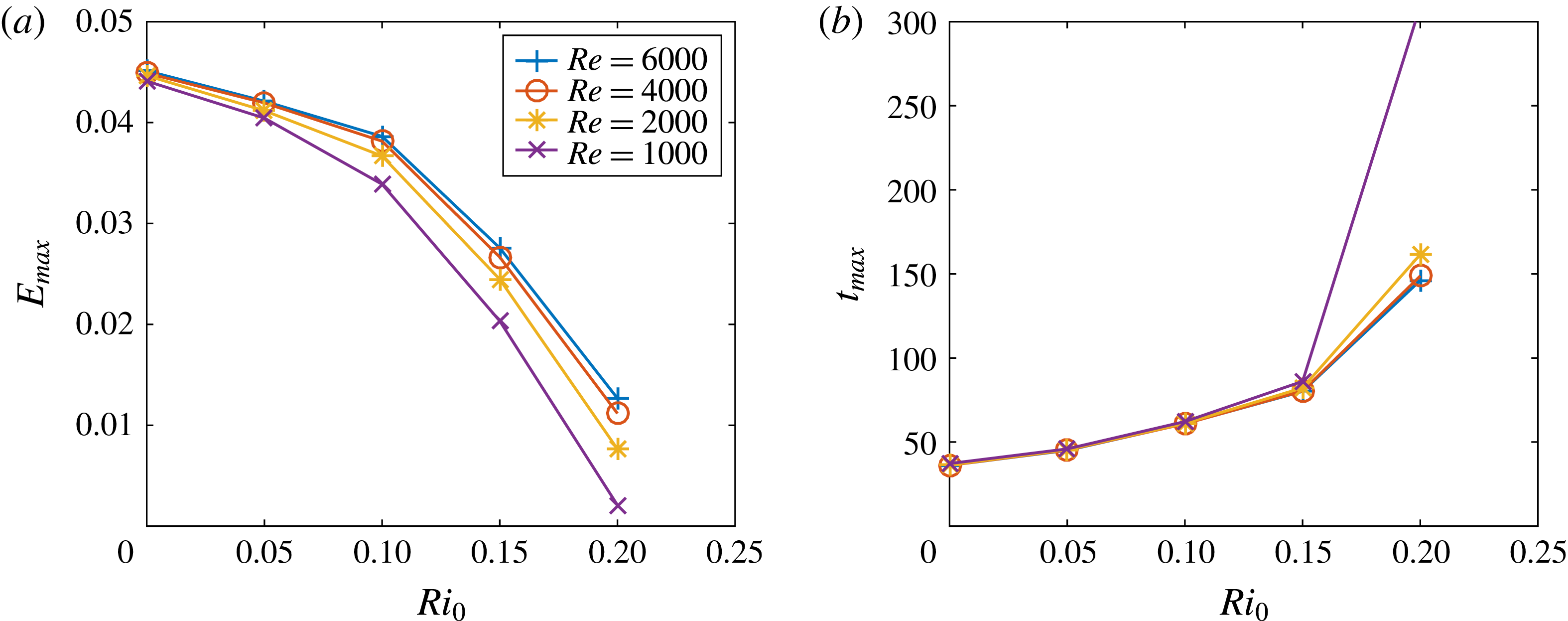
For class D simulations, variation with
 $Re$
and
 $Ri_{0}$
of (a) peak energy,
 $E_{\mathit{max}}$
, and (b) time to saturation,
 $t_{\mathit{max}}$
.

3.1 Class D: diffusing shear layers
As mentioned in the introduction, we consider three distinct classes of flow. In the first class D (simulations D1–D4 in table 1), we consider
 $Re\in [1000,6000]$
and
 $Ri_{m}\in [0,0.2]$
. We refer to this class as class D since no body forcing is added to the equations of motion and the shear layer is allowed to diffuse freely. Figure 1 shows the variation in
 $E_{\mathit{max}}$
and
 $t_{\mathit{max}}$
at the saturation point for these simulations. For all of these simulations, we choose the initial amplitude of the perturbation to be
 $E_{0}=10^{-6}$
, so that the perturbations exhibit an initial period of exponential growth, consistent with our linear stability calculations. At all
 $Re$
, increase of
 $Ri_{0}$
(and
 $Ri_{m}$
) produces a monotonic decrease in
 $E_{\mathit{max}}$
as well as a monotonic increase in
 $t_{\mathit{max}}$
. The saturation point is weakly dependent on
 $Re$
at low values of
 $Ri_{0}$
, with a 4 % decrease in
 $E_{\mathit{max}}$
between
 $Re=1000$
and
 $6000$
at
 $Ri_{0}=0.05$
. The peak energy,
 $E_{\mathit{max}}$
, decreases towards zero at higher
 $Ri_{0}$
, although there is clearly non-trivial
 $Re$
dependence. When the perturbation amplitude is still relatively close to
 $E_{0}$
, diffusion of the background profiles leads to an increase in
 $Ri_{m}$
over time. The primary effect of decreasing
 $Re$
is to speed up this process. As a consequence, at
 $Ri_{0}=0.2$
, decreasing
 $Re$
monotonically decreases
 $E_{\mathit{max}}$
and monotonically increases
 $t_{\mathit{max}}$
. Furthermore, since we define the perturbation energy as the difference from the initial velocity and buoyancy profiles defined by
 $U(z)=B(z)=\tanh (z)$
, diffusion contributes to perturbation growth. This contribution is small compared with
 $E_{\mathit{max}}$
except in the simulation
 $Re=1000$
,
 $Ri=0.2$
, for which no clear billow structure develops. In fact, the ‘saturation point’ plotted in figure 1 corresponds to the end of this simulation when the mean profiles have diffused most.
Snapshots of spanwise vorticity
 $\unicode[STIX]{x1D714}=\unicode[STIX]{x2202}_{x}w-\unicode[STIX]{x2202}_{z}u$
at times
 $t=t_{\mathit{max}}$
for class S simulations with (a)
 $Ri_{0}=0$
, (b)
 $Ri_{0}=0.1$
and (c)
 $Ri_{0}=0.245$
.

3.2 Class S: steady shear layers
It is apparent that diffusion influences the ‘saturation point’ by altering the mean velocity and density profiles, particularly for
 $Ri_{0}\simeq 1/4$
. To investigate the behaviour at higher Richardson numbers, we introduce body forces
 $F_{U}$
and
 $F_{\unicode[STIX]{x1D70C}}$
to the equations of motion to prevent diffusion of the background profiles. The governing equations become
 $$\begin{eqnarray}\displaystyle \frac{\unicode[STIX]{x2202}\boldsymbol{u}}{\unicode[STIX]{x2202}t}+\boldsymbol{u}\boldsymbol{\cdot }\unicode[STIX]{x1D735}\boldsymbol{u} & = & \displaystyle -\unicode[STIX]{x1D735}p+\frac{1}{Re}\unicode[STIX]{x1D6FB}^{2}\boldsymbol{u}+Ri_{0}\,b\,\hat{\boldsymbol{z}}+F_{U}\hat{\boldsymbol{x}},\end{eqnarray}$$
 $$\begin{eqnarray}\displaystyle \frac{\unicode[STIX]{x2202}b}{\unicode[STIX]{x2202}t}+\boldsymbol{u}\boldsymbol{\cdot }\unicode[STIX]{x1D735}b & = & \displaystyle \frac{1}{RePr}\unicode[STIX]{x1D6FB}^{2}b+F_{\unicode[STIX]{x1D70C}},\end{eqnarray}$$
 $F_{U}=F_{\unicode[STIX]{x1D70C}}=2\tanh (z)\,\text{sech}^{2}(z)/Re$
ensures that the initial background profiles
 $\bar{U}=\bar{B}=\tanh (z)$
are steady solutions. Crucially,
 $Ri_{m}$
of the background flow is then equal to
 $Ri_{0}$
throughout the initial development of the primary instability. We refer to these simulations, whose properties are listed in table 1, with
 $0\leqslant Ri_{0}\leqslant 0.245$
, as being in class S. Since variations in
 $Re$
have little effect on the subsequent evolution of the flow, we fix
 $Re=4000$
. For this class, it is natural to consider the proportion of the background kinetic energy converted to perturbation (both kinetic and potential) energy in the primary billow. At the saturation point, we therefore consider the perturbation energy density in the centre of the domain,
 $E_{c}$
, and the kinetic energy of the background flow,
 $K_{B}$
, and calculate the ratios
 $$\begin{eqnarray}R_{T}=\frac{E_{c}}{K_{B}}=R_{K}+R_{P}=\frac{E_{K}+E_{P}}{K_{B}}=\frac{{\displaystyle \frac{1}{2}}\displaystyle \int _{-3.5}^{3.5}\displaystyle \int _{0}^{L_{x}}\boldsymbol{u}^{\prime }\boldsymbol{\cdot }\boldsymbol{u}^{\prime }+Ri_{0}{b^{\prime }}^{2}\,\text{d}x\,\text{d}z}{{\displaystyle \frac{L_{x}}{2}}\displaystyle \int _{-3.5}^{3.5}\tanh ^{2}(z)\,\text{d}z},\end{eqnarray}$$
where the vertical range is chosen so that it contains all saturated billows, as is demonstrated in figure 2 for three characteristic choices of
 $Ri_{0}=0,0.1$
and
 $0.245$
. As is well known, at higher
 $Ri_{0}$
, baroclinic effects cause vorticity to become concentrated in the braid and the height of the billow to decrease (Caulfield & Peltier Reference Caulfield and Peltier2000).
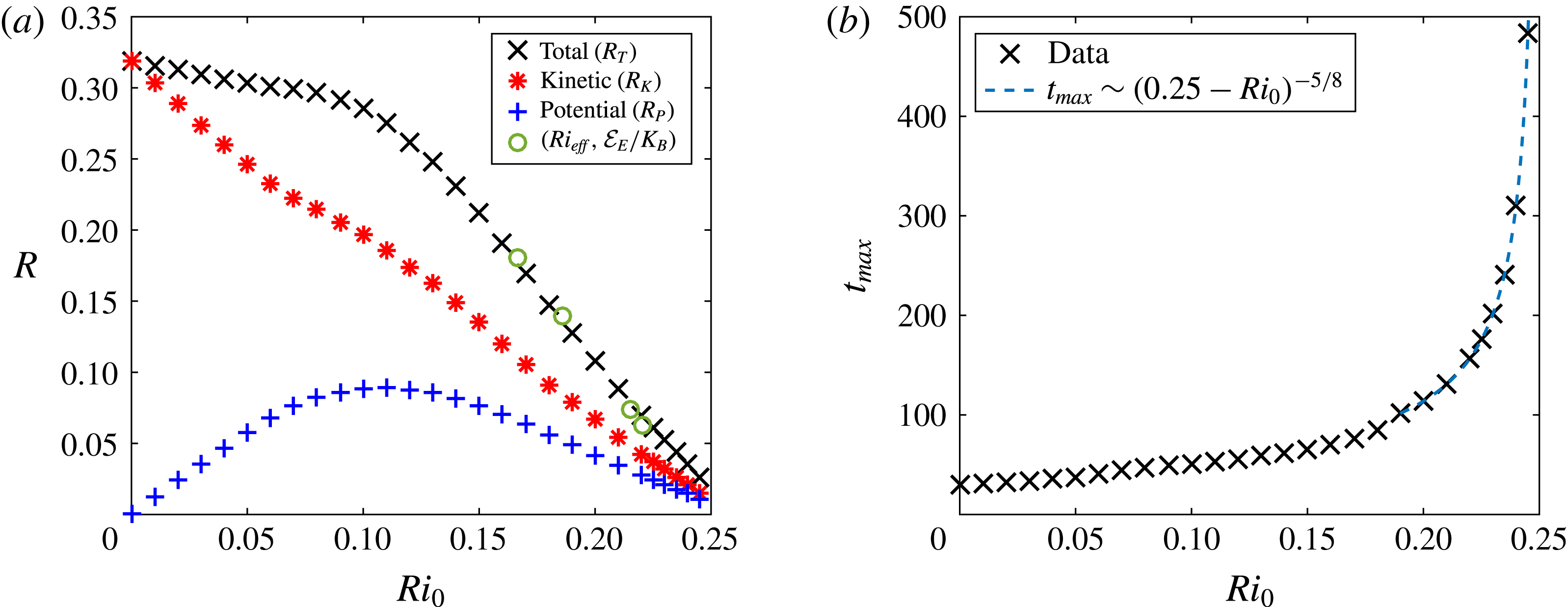
Figure 3(a) demonstrates a decreasing monotonic relationship between the total perturbation energy ratio,
 $R_{T}$
, at the saturation point and
 $Ri_{0}$
. The kinetic energy component,
 $R_{K}$
, decreases approximately linearly with increasing
 $Ri_{0}$
, whereas the potential energy component,
 $R_{P}$
, varies non-monotonically, explaining the ‘kink’ in the variation of
 $R_{T}$
with
 $Ri_{0}$
at
 $Ri_{0}\approx 0.1$
. Although we suppress diffusion of the background flows, some mixing still occurs within the billow as it rolls up, altering the mean velocity and buoyancy profiles, contributing approximately 30 % of the maximum perturbation energy. Interestingly, despite the lack of linear perturbation growth at
 $Ri_{0}=1/4$
, the various scaled perturbation energy ratios
 $R_{T}$
,
 $R_{K}$
and
 $R_{P}$
do not approach zero as
 $Ri_{0}\rightarrow 1/4$
. Figure 3(b) displays the time,
 $t_{\mathit{max}}$
, to the saturation point for this class, which appears to diverge as
 $Ri_{0}\rightarrow 1/4$
. By performing linear regression on the logarithmic values of this plot, the divergent scaling
 $t_{\mathit{max}}\sim (0.25-Ri_{0})^{-5/8}$
is provided. Crucially, it appears to be impossible to ‘store’ significant energy in a primary saturated billow from KHI when
 $Ri_{m}\lesssim 1/4$
, thus calling into question the applicability of the linear marginal stability concept to the triggering of turbulence in flows with
 $Ri_{m}\simeq 1/4$
.
For class S simulations, variation with
 $Ri_{0}$
of (a) scaled maxima of total perturbation energy
 $R_{T}$
(crosses), perturbation kinetic energy
 $R_{K}$
(asterisks) and perturbation potential energy
 $R_{P}$
(pluses) as defined in (3.2); (b)
 $t_{\mathit{max}}$
. In (a), circles mark
 $Ri_{\mathit{eff}}$
and the maximum value of
 ${\mathcal{E}}_{E}/K_{B}$
for class A simulations, as discussed in § 3.3.

3.3 Class A: accelerating shear layers
Although steady flows with
 $Ri_{m}\simeq 1/4$
appear not to be able to generate substantial saturated perturbation energy, to test the marginal stability/instability concepts it is also necessary to investigate whether time-dependent flows with decreasing Richardson numbers can lead to energetic billows as
 $Ri_{m}$
drops (slightly) below
 $1/4$
. To investigate this issue, we consider the final class A of simulations, which start in a linearly stable state with
 $Ri_{0}=0.26$
and are then accelerated by body forcing, which lowers
 $Ri_{m}$
to below
 $1/4$
. Precisely, we solve (3.1) by specifying
 $F_{\unicode[STIX]{x1D70C}}=0$
(so that buoyancy freely diffuses) and
 $$\begin{eqnarray}F_{U}=\left(\frac{2}{Re}\tanh (z)\text{sech}^{2}(z)+\unicode[STIX]{x1D6FE}\tanh (z)\right)\text{e}^{\unicode[STIX]{x1D6FE}t},\end{eqnarray}$$
which thus has an accelerating background velocity solution
 $\bar{U}=\tanh (z)\text{e}^{\unicode[STIX]{x1D6FE}t}$
. Here,
 $\unicode[STIX]{x1D6FE}$
is a forcing rate, which we prescribe as a constant between
 $10^{-5}$
and
 $2\times 10^{-3}$
. Such an accelerating background flow increases the effective Reynolds number of the flow, limiting our choice of
 $\unicode[STIX]{x1D6FE}$
to ensure that all simulations are well resolved up to the saturation point.
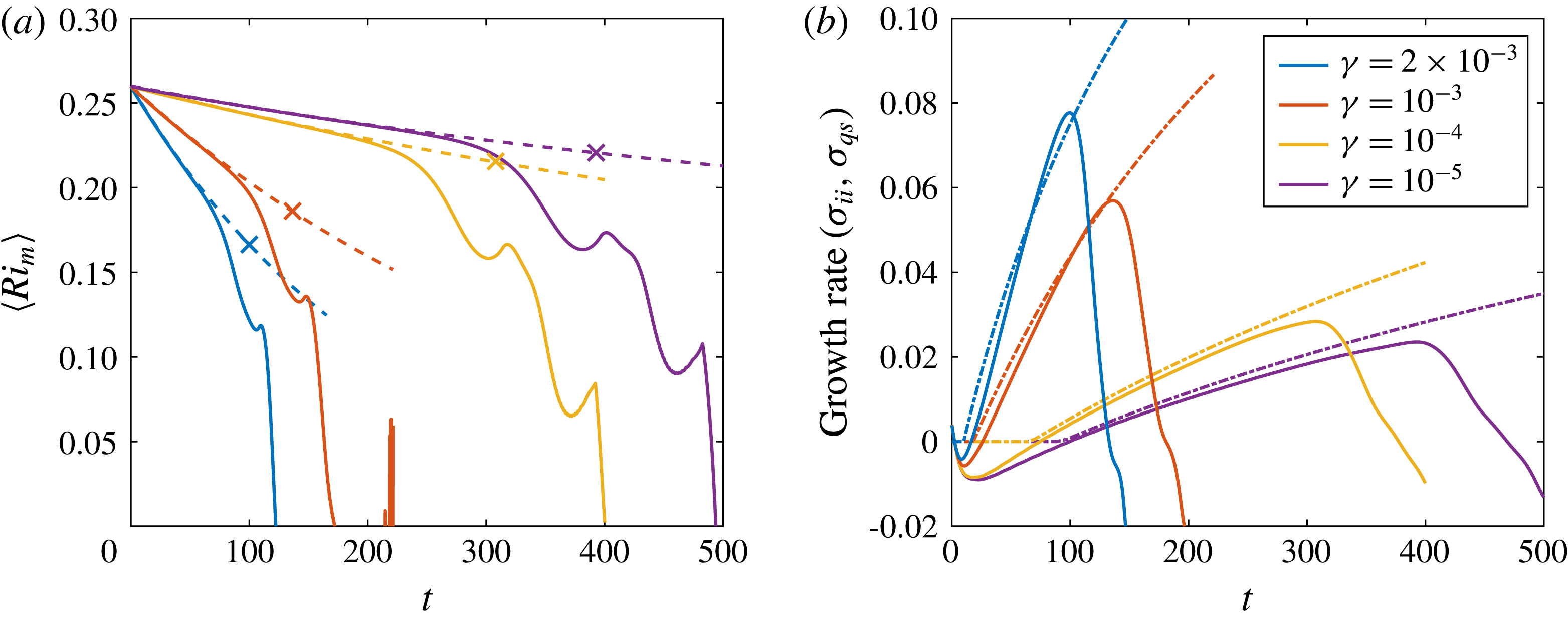
Figure 4(a) shows the effect of the forcing on the minimum mean gradient Richardson number
 $\langle Ri_{m}\rangle$
, defined by
 $$\begin{eqnarray}\langle Ri_{m}\rangle (t)=\min _{z}\langle Ri_{g}\rangle _{x}(z,t)=Ri_{0}\min _{z}\left\{\frac{\langle \unicode[STIX]{x2202}b/\unicode[STIX]{x2202}z\rangle _{x}}{\langle (\unicode[STIX]{x2202}u/\unicode[STIX]{x2202}z)^{2}\rangle _{x}}\right\},\end{eqnarray}$$
where
 $\langle \cdot \rangle _{x}$
denotes a streamwise average. Since no growing normal-mode perturbation exists for
 $Ri_{0}=0.26$
, the initial profiles are perturbed with the most unstable mode for
 $Ri_{0}=0.245$
and the length of the domain is set to the corresponding wavelength for that Richardson number. We also conduct unperturbed simulations for each forcing rate to track
 $\langle Ri_{m}\rangle$
of the purely accelerating background flow in the absence of billow formation, which is plotted with dashed lines in figure 4(a).
For comparison, we perform a linear stability analysis for a quasi-steady background flow with
 $\bar{U}=\bar{B}=\tanh (z)$
and midplane Richardson number
 $Ri_{0}=\langle Ri_{m}\rangle (t)$
. The analysis provides a predicted quasi-steady growth rate
 $\unicode[STIX]{x1D70E}_{qs}$
at each time
 $t$
and forcing rate
 $\unicode[STIX]{x1D6FE}$
, as shown in figure 4(b). Energy is added to the system by the body forcing, so the appropriate effective perturbation energy is
 $$\begin{eqnarray}{\mathcal{E}}_{E}=E_{c}[\boldsymbol{u},b]-E_{c}[\hat{\boldsymbol{u}},\hat{b}],\end{eqnarray}$$
i.e. the difference between
 $E_{c}$
for the perturbed (
 $\boldsymbol{u},b$
) and unperturbed (
 $\hat{\boldsymbol{u}},\hat{b}$
) simulations, where
 $E_{c}$
is defined in (3.2).
(a) Time series of the minimum measured Richardson number
 $\langle Ri_{m}\rangle$
from unperturbed (dashed lines) and growing (solid lines) simulations in the accelerating regime. The crosses indicate the value of
 $Ri_{\mathit{eff}}$
for each simulation, at the time
 $t_{p}$
. (b) Time series of the predicted growth rate
 $\unicode[STIX]{x1D70E}_{qs}$
from quasi-steady linear analysis (dash-dot lines) and the inferred instantaneous growth rate
 $\unicode[STIX]{x1D70E}_{ii}$
as defined in (3.6) (solid lines) for various forcing rates
 $\unicode[STIX]{x1D6FE}$
. The time
 $t_{p}$
is defined as the instant when
 $\unicode[STIX]{x1D70E}_{ii}$
is maximum.

If the flow is linearly unstable,
 $\boldsymbol{u}^{\prime },b^{\prime }\sim \text{e}^{\unicode[STIX]{x1D70E}t}$
, or, equivalently,
 ${\mathcal{E}}_{E}\sim \text{e}^{2\unicode[STIX]{x1D70E}t}$
. We can therefore test the accuracy of the linear stability analysis by calculating an inferred instantaneous growth rate from the perturbed nonlinear simulations,
 $$\begin{eqnarray}\frac{1}{2{\mathcal{E}}_{E}}\frac{\text{d}{\mathcal{E}}_{E}}{\text{d}t}=\unicode[STIX]{x1D70E}_{ii}.\end{eqnarray}$$
The solid lines in figure 4(b) show this inferred instantaneous growth rate
 $\unicode[STIX]{x1D70E}_{ii}$
. Once the predicted quasi-steady growth rate
 $\unicode[STIX]{x1D70E}_{qs}$
becomes non-zero, the inferred instantaneous growth rate
 $\unicode[STIX]{x1D70E}_{ii}$
matches the quasi-steady linear prediction
 $\unicode[STIX]{x1D70E}_{qs}$
well for a certain period of time. For each choice of forcing rate
 $\unicode[STIX]{x1D6FE}$
,
 $\unicode[STIX]{x1D70E}_{ii}$
reaches a peak at some time
 $t_{p}$
where nonlinear effects start to become significant, before falling through zero at the saturation point, when the effective perturbation energy
 ${\mathcal{E}}_{E}$
is maximum. Interestingly, for this class of flows, the effective perturbation energy
 ${\mathcal{E}}_{E}$
at the instant when the growth rate peaks is approximately 0.75 % of the initial background energy
 $K_{B}$
, independent of the forcing rate. Simulations in class S also appear to deviate from purely ‘linear’ exponential-in-time perturbation growth for a similar ratio of perturbation energy to background energy
 $K_{B}$
. The remaining perturbation growth depends on the effective Richardson number
 $Ri_{\mathit{eff}}$
, i.e. the value of
 $\langle Ri_{m}\rangle$
in the unperturbed flow at the time instant
 $t_{p}$
when
 $\unicode[STIX]{x1D70E}_{ii}$
reaches its peak value in the (perturbed) simulations, marked with crosses in figure 4(a). The maximum value of the appropriately scaled perturbation energy
 ${\mathcal{E}}_{E}/K_{B}$
at the saturation points is plotted (with circles) against
 $Ri_{\mathit{eff}}$
in figure 3(a), showing striking agreement with the simulations in the steady class S. It appears that the maximum amplitude of the nonlinear billow state is controlled by the minimum value of
 $Ri_{g}$
of the background flow relatively early in the development of the instability (specifically when nonlinear effects start to reduce the inferred instantaneous growth rate), and that this maximum amplitude is very small when the relevant
 $Ri_{0}\simeq 1/4$
, even in accelerating flows.
4 Discussion and conclusions
We have performed three classes of two-dimensional direct numerical simulations of stratified shear layers susceptible to KHI: class D, where the background flow profiles are free to diffuse; class S, where body forcings allow the initial background flow profiles to be steady solutions of the governing equations; and class A, where the background velocity profile accelerates. In each class, the saturated amplitude of the nonlinear billow state decreases as the initial minimum gradient Richardson number,
 $Ri_{m}$
, increases. In class D,
 $Re$
becomes important as
 $Ri_{m}\rightarrow 1/4$
since diffusion of the background flow increases the Richardson number to a linearly stable value. For class S, where body forcing keeps
 $Ri_{m}$
constant, a clear monotonic relationship arises between
 $Ri_{m}$
and the saturated amplitude of the nonlinear state. The time at which this saturated amplitude occurs diverges as
 $Ri_{m}\rightarrow 1/4$
, while the saturated amplitude of the billow decreases to a small but non-zero value. This limit yields flattened billows, as shown in figure 2(c). It is important to appreciate that these results are not direct consequences of the Miles–Howard criterion, which only considers the exponential growth of infinitesimal perturbations on steady inviscid flows and not the properties of potentially ensuing nonlinear states.
We find that the instabilities that develop in the accelerating shear layers of class A are still, at early times, well described by quasi-steady linear stability analyses using an instantaneous Richardson number. The saturated energy of these billows is still consistent with the relationship shown in figure 3(a), reaffirming that the saturated amplitude is restricted by
 $Ri_{m}$
. We find that nonlinear effects become important when a perturbation reaches an amplitude corresponding to 0.75 % of the initial background kinetic energy.
We conclude that these results are not consistent with the connection between marginally unstable flow states and the generation or ‘triggering’ of turbulence through unstable linear normal-mode disturbances. In particular, the application of the Miles–Howard criterion to provide a stability boundary for naturally occurring turbulent shear flows appears to be inconsistent with the demonstrated nonlinear development of KHI in laminar states at high
 $Re$
. Indeed, our results are broadly consistent with studies of internal solitary waves, which have similarly suggested that wave breaking requires the minimum Richardson number in the pycnocline to be below approximately 0.1 (Lamb Reference Lamb2014). We hypothesise that vigorous energy injection to finite amplitude structures that have the potential to trigger turbulent transition requires minimum Richardson numbers within the flow to be substantially below
 $1/4$
.
This hypothesis is not inconsistent with the observations discussed by Thorpe & Liu (Reference Thorpe and Liu2009) and Smyth & Moum (Reference Smyth and Moum2013), since we are concerned with the laminar states required for turbulent transition rather than the ensuing turbulent flow itself. However, the use of linear stability analysis by Thorpe & Liu (Reference Thorpe and Liu2009) and Thorpe et al. (Reference Thorpe, Smyth and Li2013) to determine the stability of turbulent shear flows by the Miles–Howard criterion does not appear to be valid given our results. Since the nonlinear structures that develop in our marginally unstable laminar flows are very small and take a long time to saturate, any linear perturbation in a similarly marginal turbulent flow is likely to be strongly influenced by the surrounding turbulence. This introduces uncertainty to both the development of a linear perturbation and the nature of its finite amplitude manifestation as a nonlinear billow structure. We conclude that the application of marginal stability to naturally occurring turbulent flows should be based on results concerning the growth and decay of stratified turbulence around certain Richardson numbers (e.g. Rohr et al. Reference Rohr, Itsweire, Helland and Atta1988; Zhou, Taylor & Caulfield Reference Zhou, Taylor and Caulfield2017), rather than linear stability arguments.
Although we have only performed simulations in a two-dimensional domain, we remain confident that our results have relevance to fully three-dimensional realisations of these flows. By computing the turbulent kinetic energy of the class S simulations, we obtain comparable values at saturation to those found in figure 3(b) of the three-dimensional study of Mashayek et al. (Reference Mashayek, Caulfield and Peltier2013). The peak energy we obtain takes slightly higher values than those of Mashayek et al. (Reference Mashayek, Caulfield and Peltier2013) because of the reduced diffusion keeping the minimum Richardson number at a lower value in our case. For our highest
 $Ri_{0}$
values, no three-dimensional studies have been performed, but Mashayek & Peltier (Reference Mashayek and Peltier2012b
) found that the growth rates of all secondary instabilities decrease as
 $Ri_{0}$
is increased past 0.12. We therefore believe that the behaviour of the two-dimensional roll-up is still important at higher
 $Ri_{0}$
.
It is important to remember that we have only considered the nonlinear development of a linear normal-mode perturbation. As noted in the introduction, Kaminski et al. (Reference Kaminski, Caulfield and Taylor2017) have shown that sufficiently large-amplitude perturbations with the structure of a linear optimal perturbation can still develop into a ‘Kelvin–Helmholtz-like’ billow state for flows with
 $Ri_{m}$
as high as 0.4, which may perhaps explain why the maximum energy in figure 3(a) does not tend to zero as
 $Ri_{m}\rightarrow 1/4$
. Indeed, with a specific type of large forcing, a saturated nonlinear overturning billow structure may possibly develop at
 $Ri_{m}=1/4$
through a different (and inherently transient non-normal) mechanism, distinct from perturbation by a classical normal-mode linear instability.
Although flows in the atmosphere or oceans are far more complex than those considered here, our results from time-dependent shear layers (class A) suggest that minimum values of
 $Ri_{g}$
directly control the saturated amplitude of Kelvin–Helmholtz billows. In particular, we have shown that the time for the perturbation energy to saturate becomes very long as
 $Ri_{m}\rightarrow 1/4$
, and the billow amplitude is small in this limit, implying that a laminar flow in this state is unlikely to become turbulent. For example, use of a typical value of 1 m for a shear layer half-depth, and a velocity difference of
 $2U_{0}^{\ast }=7.5\times 10^{-2}\text{ms}^{-1}$
from measurements by van Haren & Gostiaux (Reference van Haren and Gostiaux2010) to calculate an advective time scale gives
 $t_{\mathit{max}}$
greater than 22 min for
 $Ri_{0}\geqslant 0.2$
. At
 $Ri_{0}=0.24$
, the appropriately scaled saturation time becomes longer than an hour. Further work to examine the effect of ambient turbulence or internal waves on the saturated billow amplitudes would be invaluable for quantification of the potential for enhanced mixing and turbulence of shear-driven overturning structures in the ocean.
Acknowledgements
We thank three anonymous referees whose thoughtful and constructive comments have substantially improved this paper. C.J.H. is supported by the Cambridge Earth System Science NERC DTP (NE/L002507/1). The research activity of J.R.T. and C.P.C. is supported by EPSRC Programme Grant EP/K034529/1 entitled ‘Mathematical Underpinnings of Stratified Turbulence’ (MUST). Valuable discussions with the rest of the MUST team are gratefully acknowledged. The data used to create figures 1, 3 and 4, and the initial condition header data for Diablo for the simulations outlined in table 1 are available at https://doi.org/10.17863/CAM.17349.