2.1. Fluidic oscillator operating principle

The typical structure of the targeted fluidic oscillator comprises an inlet, a mixing chamber, two feedback channels and an outlet, as shown in figure 1(a); the configuration was adapted from Ostermann et al. (Reference Ostermann, Woszidlo, Nayeri and Paschereit2018). When fluid enters the mixing chamber, the Coanda effect causes the jet to attach to one sidewall, as shown by the two fully attached states in figure 1(b). A portion of this attached flow is diverted into the feedback channel on the same side and returned to the inlet region. This feedback flow entrains the main jet near the chamber inlet, prompting it to adhere rapidly to the opposite wall. This deflection results in a change in the jet direction at the outlet. Owing to the symmetrical design of the oscillator, this process repeats continuously, establishing a self-sustaining oscillation and generating a periodic sweeping jet at the outlet. Accordingly, the subsequent modelling is based on this working principle and focuses on the Coanda effect and feedback mechanism.

Figure 1.

(a) Basic structure of the fluidic oscillator, featuring a mixing chamber and dual-feedback channels. (b) The two jet attachment states, with red and blue lines indicating attachment to the left and right walls of the mixing chamber, respectively.

2.2. Integral form of the momentum equation in non-inertial reference frames

Based on previous research, it is understood that the feedback recirculation constitutes the primary cause of jet oscillation (Woszidlo et al. Reference Woszidlo, Ostermann, Nayeri and Paschereit2015; Wen & Liu Reference Wen and Liu2018). Furthermore, the mixing chamber is the primary site of jet attachment, making its analysis crucial for understanding the oscillation mechanism. This study assumes that the flow within the fluidic oscillator is two-dimensional, incompressible and inviscid, and that the main jet maintains a constant width. Based on these assumptions, the main jet in the mixing chamber was analysed using the concept of a fluid parcel (i.e. a control volume). A simplified configuration of the oscillator, developed from the baseline design in figure 1, is presented in figure 2. This idealised model preserves the core geometry while offering greater analytical tractability. The control volume of the fluid parcel is defined at the jet, with its lateral boundaries aligned with the edges of the jet. Its dimensions are the width $w$ (equal to the jet width) and height $\text{d}y$ .

Figure 2.

Fluidic oscillator and its jet fluid parcel.

The momentum equation in the x-direction for the control volume (in the absolute coordinate system) is as follows:

(2.1) \begin{equation} \frac{\partial \left(V_{x}\mathrm{d}m\right)}{\partial t}=V_{xL}\mathrm{d}\dot{m}_{L}-V_{xR}\mathrm{d}\dot{m}_{R}+\sum \mathrm{d}F_{x} ,\end{equation}

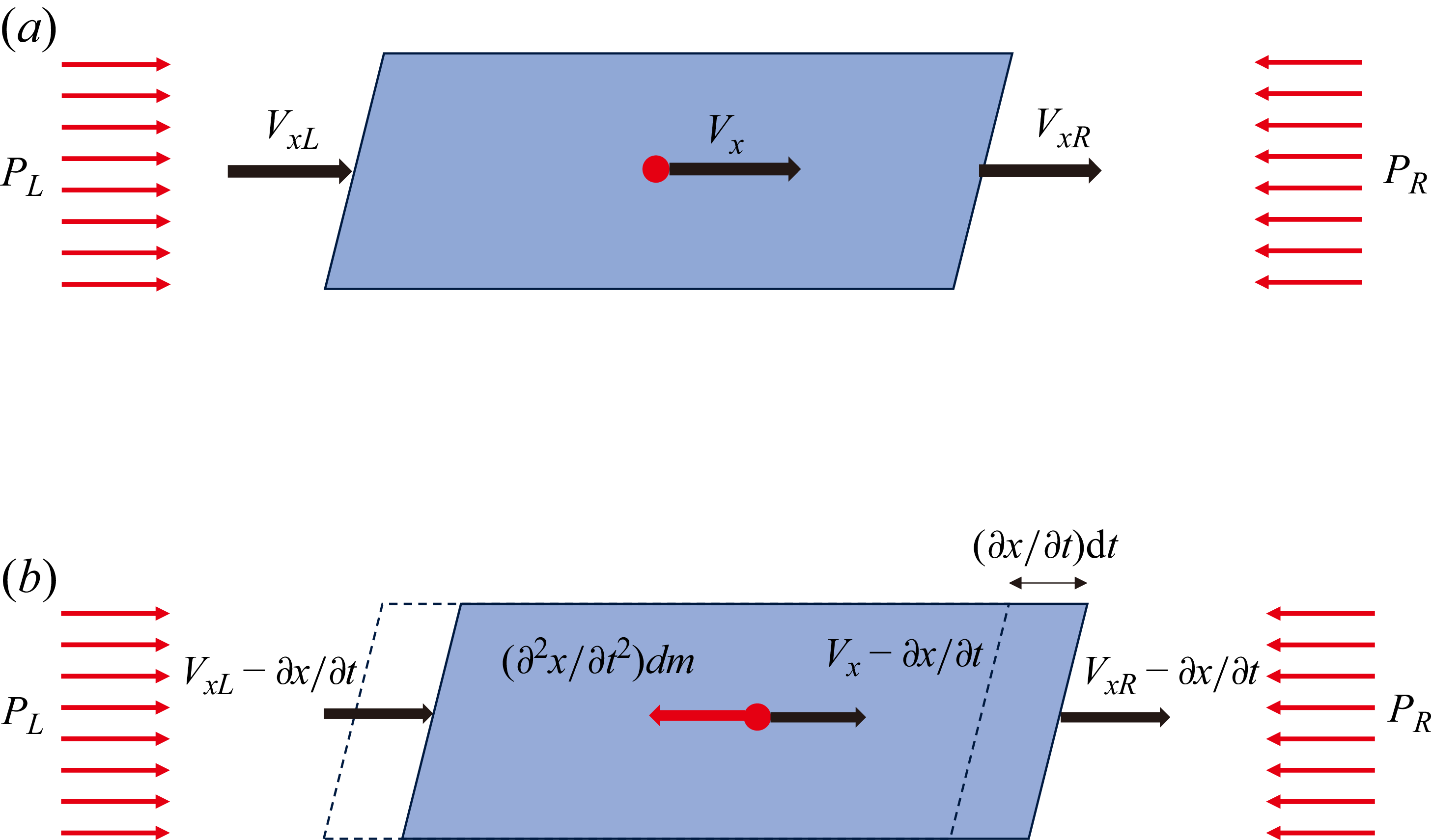
where $V_{x}$ is the horizontal velocity, $\mathrm{d}m$ is the mass of a fluid parcel, $\mathrm{d}\dot{m}$ is the mass flow rate at the parcel boundary and $\mathrm{d}F_{x}$ is the contribution of the body or surface forces to the momentum. The subscripts L and R denote the left and right boundaries of the control volume, respectively. The reference frame of the control volume is set to oscillate synchronously with the jet in the x-direction (i.e. remaining relatively stationary to the jet), ensuring that the left and right boundaries of the control volume always coincide with the corresponding jet boundaries. Therefore, when formulating the momentum equation in the x-direction, the relative velocity must be calculated by subtracting the horizontal velocity of the reference frame. Figure 3 illustrates the velocities and forces acting on a fluid parcel in the x-direction, represented in both the absolute and relative frame of reference. Based on this diagram, (2.1) can be rewritten as

(2.2) \begin{equation} \frac{\partial \left[\left(V_{x}-\dfrac{\partial x}{\partial t}\right)\mathrm{d}m\right]}{\partial t}=\left(V_{xL}-\frac{\partial x}{\partial t}\right)\mathrm{d}\dot{m}_{L}-\left(V_{xR}-\frac{\partial x}{\partial t}\right)\mathrm{d}\dot{m}_{R}+\sum \mathrm{d}F_{x} ,\end{equation}

where ${\partial x}/{\partial t}$ represents the horizontal velocity of the reference frame and $V_{x}-{\partial x}/{\partial t}$ denotes the resultant relative velocity. In addition, $x(y,t)$ is a function of $y$ and $t$ representing the time-varying x-coordinate of the jet centreline. Under the incompressible flow assumption, the mass in the control volume (assuming the thickness in the z-direction is 1) is $\mathrm{d}m=\rho w\mathrm{d}y$ . The mass flow rates are $\mathrm{d}\dot{m}_{L}=\rho (V_{xL}-({\partial x}/{\partial t}))\mathrm{d}y$ and $\mathrm{d}\dot{m}_{R}=\rho (V_{xR}-({\partial x}/{\partial t}))\mathrm{d}y$ , where $\rho$ represents the fluid density. Given the expressions of $\mathrm{d}m , \mathrm{d}\dot{m}_{L}$ and $\mathrm{d}\dot{m}_{R}$ , substitution into (2.2) yields

(2.3) \begin{equation} \rho w\frac{\partial \left(V_{x}-\dfrac{\partial x}{\partial t}\right)}{\partial t}\text{d}y=\rho \left[\left(V_{xL}-\frac{\partial x}{\partial t}\right)^{2}-\left(V_{xR}-\frac{\partial x}{\partial t}\right)^{2}\right]\text{d}y+\sum \mathrm{d}F_{x} .\end{equation}

Here, $\sum \mathrm{d}F_{x}$ primarily comprises inertial and pressure forces

(2.4) \begin{equation} \sum \mathrm{d}F_{x}=-\frac{\partial ^{2}x}{\partial t^{2}}\mathrm{d}m+\left(P_{L}-P_{R}\right)\mathrm{d}y ,\end{equation}

where $P_{L}$ and $P_{R}$ denote the pressures on the left and right boundaries of the control volume, respectively, and $-{\partial ^{2}x}/{\partial t^{2}}\mathrm{d}m$ corresponds to the inertial force of the fluid within the control volume. Therefore, combining Equations (2.3) and (2.4) yields

(2.5) \begin{align} \rho w\frac{\partial ^{2}x}{\partial t^{2}}\mathrm{d}y+\rho w\frac{\partial \left(V_{x}-{\partial x}/{\partial t}\right)}{\partial t}\text{d}y&=\left(P_{L}-P_{R}\right)\mathrm{d}y+\rho \left[\left(V_{xL}-\frac{\partial x}{\partial t}\right)^{2}\right .\nonumber\\&\quad \left .-\left(V_{xR}-\frac{\partial x}{\partial t}\right)^{2}\right]\mathrm{d}y ,\end{align}

where the functions $x(y,t) , P_{L}(y,t) , P_{R}(y,t) , V_{x}(y,t) , V_{xL}(y,t)$ and $V_{xR}(y,t)$ are all dependent on $y$ and $t$ . These functions are assumed to be continuous and differentiable; thus, the order of integration and differentiation can be interchanged. Under these assumptions, integrating (2.5) along the y-direction over the interval $[0,L_{m}]$ (i.e. across the mixing chamber length) yields

(2.6) \begin{align} & w\frac{\text{d}^{2}}{\text{d}t^{2}}\!\int _{0}^{L_{m}}\!x(y,t)\, \text{d}y+w\frac{\text{d}}{\text{d}t}\int _{0}^{L_{m}}\left[\!V_{x}-\frac{\partial x(y,t)}{\partial t}\!\right] \text{d}y =\frac{1}{\rho }\!\int _{0}^{L_{m}}\!\left[P_{L}(y,t)-P_{R}(y,t)\right] \text{d}y \nonumber\\ &\quad +\int _{0}^{L_{m}}\left[\left(V_{xL}-\frac{\partial x}{\partial t}\right)^{2}-\left(V_{xR}-\frac{\partial x}{\partial t}\right)^{2}\right] \text{d}y . \end{align}

Figure 3.

Schematic diagram of the velocity and forces acting on a fluid parcel in the x-direction under two coordinate systems. (a) Absolute frame of reference and (b) relative frame of reference.

To simplify (2.6), we define

(2.7) \begin{equation} \left\{\!\!\begin{array}{l} \displaystyle \int _{0}^{L_{m}}x(y,t)\text{d}y=b_{0}L_{m}\overline{x}\left(t\right),\\[9pt] \displaystyle \int _{0}^{L_{m}}\left[P_{L}(y,t)-P_{R}(y,t)\right] \text{d}y={\unicode[Arial]{x0394}} \overline{P}\left(t\right)L_{m}, \end{array}\right. \end{equation}

where $\overline{x}(t)$ ranges over the interval $[-{w_{m}}/{2},{w_{m}}/{2}]$ . Physically, $\int _{0}^{L_{m}}x(y,t)\text{d}y$ represents the area enclosed between the jet centreline and centreline of the fluidic oscillator. A correction factor $b_{0} (0\lt b_{0}\lt 1)$ is introduced to ensure that the value of $\overline{x}(t)$ lies within the interval $[-{w_{m}}/{2},{w_{m}}/{2}]$ . The variable ${\unicode[Arial]{x0394}} \overline{P}(t)$ represents the average pressure difference between both sides of the jet within the mixing chamber. Substituting (2.7) into (2.6) yields the momentum equation for the fluidic oscillator in a non-inertial frame

(2.8) \begin{align} & wb_{0}L_{m}\frac{\text{d}^{2}\overline{x}\left(t\right)}{\text{d}t^{2}}+w\frac{\text{d}}{\text{d}t}\int _{0}^{L_{m}}\left[V_{x}-\frac{\partial x(y,t)}{\partial t}\right] \text{d}y =\frac{1}{\rho }{\unicode[Arial]{x0394}} \overline{P}\left(t\right)L_{m}\nonumber\\&\quad +\int _{0}^{L_{m}}\left[\left(V_{xL}-\frac{\partial x}{\partial t}\right)^{2}-\left(V_{xR}-\frac{\partial x}{\partial t}\right)^{2}\right] \text{d}y. \end{align}

As outlined above, the integral form of the horizontal momentum conservation equation for the control volume comprises several key components: inertial force, unsteady term, pressure force and momentum flux. The primary components of this equation will be simplified or modelled in subsequent sections.

2.3. Approximation of the unsteady term

Before simplifying the unsteady term in the momentum equation, it is necessary to clarify that the horizontal flow velocity $V_{x}(y,t)$ in a fluid parcel differs from that of the control volume in the x-direction (i.e. ${\partial x}/{\partial t}$ ) at a certain position of $y$ within the main jet. This discrepancy arises because of the y-direction movement (at the velocity of $V_{j}$ ) of the fluid parcel. Figure 4 illustrates the displacement variation of the fluid parcel at different time instants. Based on the relationships shown in the figure, the following equation can be derived:

(2.9) \begin{align} \frac{\partial x(y,t)}{\partial t}&=\frac{x\left(y,t+\text{d}t\right)-x(y,t)}{\text{d}t}=\frac{V_{x}\text{d}t-\left[x(y,t)-x\left(y-V_{j}\text{d}t,t\right)\right]}{\text{d}t}\nonumber\\& =V_{x}-V_{j}\frac{\partial x(y,t)}{\partial y} . \end{align}

Figure 4.

The evolution of jet fluid parcel positions.

Substituting this relation into the unsteady term of (2.8) yields

(2.10) \begin{align} w\frac{\text{d}}{\text{d}t}\int _{0}^{L_{m}}\left[V_{x}-\frac{\partial x(y,t)}{\partial t}\right] \text{d}y =w\frac{\text{d}}{\text{d}t}\left[V_{j}\int _{0}^{L_{m}}\frac{\partial x(y,t)}{\partial y} \text{d}y\right]\! . \end{align}

As shown in figure 2, given the symmetry of the mixing chamber about $y=0.5L_{m}$ , we assumed that the jet shape within it was also symmetric about this line. Thus, $(\partial x(y,t)/\partial y)\approx -(\partial x(L_{m}-y,t)/\partial y)$ can be derived, and $\int _{0}^{L_{m}}{\partial x(y,t)}/{\partial y}\,\text{d}y\approx 0$ . This implies that the unsteady term in the momentum equation was approximately zero

(2.11) \begin{equation} w\frac{\text{d}}{\text{d}t}\int _{0}^{L_{m}}\left(V_{x}-\frac{\partial x}{\partial t}\right)\text{d}y\approx 0 .\end{equation}

2.4. Modelling of the momentum flux or feedback force contributions

This section models the momentum flux term. Outside the jet and the vicinity of the inlets and outlets of feedback channels, the flow in the mixing chamber is characterised by a separation bubble with low velocity that is negligible compared with the jet. Therefore, the flow in these regions can be approximately considered as being in a stationary state (i.e. $v_{xL}\approx 0 , v_{xR}\approx 0$ within the range $y\in [w_{\!f},L_{m}-w_{\!f}]$ ), where $(V_{xL}-{\partial x}/{\partial t})^{2}-(V_{xR}-{\partial x}/{\partial t})^{2}\approx 0$ .

In the region near the inlets and outlets of the feedback channels (i.e. $y\in [0,w_{\!f}]\cup [L_{m}-w_{\!f},L_{m}]$ ), the primary jet is in close proximity to the inlets and outlets of the mixing chamber (see figure 2). Analogous to the fixed ends of a vibrating string, where the displacement remains zero, the horizontal displacement of fluid parcels at these locations is also negligible (i.e. $x(0,t)\approx 0$ and $x(L_{m},t)\approx 0$ ). Thus, when $y\in [0,w_{\!f}]\cup [L_{m}-w_{\!f},L_{m}]$ , it is assumed that ${\partial x}/{\partial t}\approx 0$ , thereby yielding

(2.12) \begin{align} \left(V_{xL}-\frac{\partial x}{\partial t}\right)^{2}-\left(V_{xR}-\frac{\partial x}{\partial t}\right)^{2} \approx \left({V_{xL}}^{2}-{V_{xR}}^{2}\right)\! . \end{align}

During the oscillation of the jet within the mixing chamber, the feedback flow in the left and right feedback channels typically exhibits pulsating fluctuations (Joulaei et al. Reference Joulaei, Nili-Ahmadabadi and Kim2022; Iskandar et al. Reference Iskandar, Julian and Chern2025). The flow velocities in the right and left feedback channels, denoted as $V_{\textit{f{\kern1pt}R}}$ and $V_{\textit{f{\kern1pt}L}}$ , respectively, were defined as positive from the channel inlet to the outlet. Based on the incompressibility assumption, the flow velocities in one feedback channel must be equal. These can be decomposed into time-averaged and fluctuating components

(2.13) \begin{equation} \left\{\!\!\begin{array}{l} V_{\textit{f{\kern1pt}L}}\left(t\right)=\overline{V}_{\textit{f{\kern1pt}L}}+v_{\textit{f{\kern1pt}L}}\left(t\right),\\ V_{\textit{f{\kern1pt}R}}\left(t\right)=\overline{V}_{\textit{f{\kern1pt}R}}+v_{\textit{f{\kern1pt}R}}\left(t\right) ,\end{array}\right. \end{equation}

where the values $\overline{V_{\!f}}$ and $v_{\!f}$ represent the time-averaged and fluctuating components of the feedback flow, respectively, and the subscripts L and R denote the left and right feedback channels, respectively. Seo et al. (Reference Seo, Zhu and Mittal2018) observed a distinct phase difference of half the oscillation period (T/2) between pulsating flows in the left and right feedback channels. They further established that the phase of the differential flow rate between these channels aligns with the oscillation phase in the mixing chamber, leading them to conclude that the fluctuating component of the feedback flow is the crucial driver of the fluidic oscillation. Owing to the symmetry of the fluidic oscillator, the time-averaged components of $\overline{V}_{\!fL}$ and $\overline{V}_{\!fR}$ , which primarily constitute a time-averaged flow field symmetric about the y-axis, oppose and cancel each other at the ends of the mixing chamber, and thus do not contribute to the jet oscillation. Therefore, the fluctuating components of $v_{\!fL}(t)$ and $v_{\!fR}(t)$ were identified as the dominant factors driving the oscillator operation. If both the inlet and outlet of the feedback channel have a width of $w_{\!f}$ , the momentum flux of (2.12) yields

(2.14) \begin{align} \int _{0}^{L_{m}}\left[\left(V_{xL}-\frac{\partial x}{\partial t}\right)^{2}-\left(V_{xR}-\frac{\partial x}{\partial t}\right)^{2}\right] \text{d}y &\approx \int _{0}^{w_{\!f}}\left({V_{xL}}^{2}-{V_{xR}}^{2}\right) \text{d}y \nonumber\\ +\int _{L_{m}-w_{\!f}}^{L_{m}}\left({V_{xL}}^{2}-{V_{xR}}^{2}\right) \text{d}y & \approx 2w_{\!f}\left({v_{xL}}^{2}-{v_{xR}}^{2}\right)\!. \end{align}

We further hypothesised that the oscillation of the main jet within the mixing chamber was influenced by the feedback channel on the same side. This implies that

(2.15) \begin{equation} 2w_{\!f}\left({v_{xL}}^{2}-{v_{xR}}^{2}\right)\approx \left\{\!\!\begin{array}{l} -2w_{\!f}{v_{\!fR}}^{2},\,\overline{x}\gt 0,\\[3pt] 2w_{\!f}{v_{\!fL}}^{2},\,\overline{x}\lt 0. \end{array}\right. \end{equation}

It is hypothesised that when the jet deflects towards one feedback channel, the pressure at the inlet of that channel increases to generate a positive feedback flow. Under this hypothesis, let

(2.16) \begin{equation} v_{\!f}=\left\{\!\!\begin{array}{l} v_{\!fR}\gt 0,\,\overline{x}\gt 0,\\ -v_{\!fL}\lt 0,\,\overline{x}\lt 0, \end{array}\right. \end{equation}

it follows that (2.15) transforms into

(2.17) \begin{equation} 2w_{\!f}\left({v_{xL}}^{2}-{v_{xR}}^{2}\right)\approx -2w_{\!f}\left| v_{\!f}\right| v_{\!f} .\end{equation}

The feedback channel flow fluctuating velocity $v_{\!f}$ is directly proportional to the jet velocity $V_{j}$ , while $\overline{x}$ captures the phase information of the $v_{\!f}$ . Research on the inlet jet angle and feedback channel flow rate confirmed this relationship (Seo et al. Reference Seo, Zhu and Mittal2018). Therefore, $v_{\!f}(t)$ should be a function of $V_{\!j}$ and $\overline{x}$ (i.e. $v_{\!f}(V_{j},\overline{x}(t))$ ), demonstrating a positive correlation with both $V_{\!j}$ and $| \overline{x}|$ . For simplicity, this study defines

(2.18) \begin{equation} \left\{\!\!\begin{array}{l} v_{\!f}\left(V_{j},\overline{x}\right)=c_{1}\left(\overline{x}\right)V_{j},\\ f\left(V_{j},\overline{x}\right)=\left| v_{\!f}\right| v_{\!f}=\left| c_{1}\left(\overline{x}\right)\right| c_{1}\left(\overline{x}\right)V_{j}^{2}=f_{c}\left(\overline{x}\right)V_{j}^{2}, \end{array}\right. \end{equation}

where the function $f_{c}(\overline{x})$ possesses two key properties. In the first property, since there is virtually no feedback backflow within the fluidic oscillator when the jet is at the centreline ( $\overline{x}=0$ ) of the mixing chamber, it follows that $f(V_{j},0)\approx 0$ . The second property follows from the combination of (2.16) and (2.18)

(2.19) \begin{equation} \left\{\!\!\begin{array}{l} \overline{x}\gt 0,v_{\!f}\gt 0,\,f\left(V_{j},\overline{x}\right)=v_{\!f}^{2}\gt 0,\\ \overline{x}\lt 0,v_{\!f}\lt 0,\,f\left(V_{j},\overline{x}\right)=-v_{\!f}^{2}\lt 0 .\end{array}\right. \end{equation}

Therefore, by symmetry, $f(V_{j},-\overline{x})=-f(V_{j},\overline{x})$ . Substituting these properties into (2.18) yields expressions of $f_{c}(0)=0$ and $f_{c}(-\overline{x})=-f_{c}(\overline{x})$ . This study further applies a Taylor series expansion about $\overline{x}=0$ to the relevant terms in (2.18). Subsequently, non-dimensionalisation was performed using the mixing chamber half-width ( $w_{m}$ /2), yielding

(2.20) \begin{equation} f_{c}\left(\overline{x}\right)=f_{c}\left(0\right)+2a_{1}\frac{\overline{x}}{w_{m}}+4a_{2}\frac{\overline{x}^{2}}{w_{m}^{2}}+8a_{3}\frac{\overline{x}^{3}}{w_{m}^{3}}+16a_{4}\frac{\overline{x}^{4}}{w_{m}^{4}}+\cdots ,\end{equation}

where $a_{k}$ is the kth coefficient in the Taylor series expansion. Substituting $f_{c}(0)=0$ and $f_{c}(-\overline{x})=-f_{c}(\overline{x})$ into the above expression and retaining the first-order terms yields

(2.21) \begin{equation} f_{c}\left(\overline{x}\right)\approx 2a_{1}\frac{\overline{x}}{w_{m}} .\end{equation}

Finally, substituting (2.18) and (2.21) into the feedback force term of (2.17) yields

(2.22) \begin{equation} \int _{0}^{L_{m}}\left[\left(V_{xL}-\frac{\partial x}{\partial t}\right)^{2}-\left(V_{xR}-\frac{\partial x}{\partial t}\right)^{2}\right] \text{d}y \approx -2w_{\!f}\left| v_{\!f}\right| v_{\!f}\approx -4a_{1}\frac{w_{\!f}}{w_{m}}V_{j}^{2}\overline{x} . \end{equation}

2.5. Modelling of the pressure force or the wall-attachment effect term

This section models the pressure force term in (2.8). As this term represents the pressure difference between the two sides of the main jet, the attachment behaviour of the jet within the mixing chamber becomes particularly important. It is well established that under non-oscillating or stable conditions, the pressures on both sides of the primary jet remain nearly identical owing to symmetry. This implies that the pressure difference term in (2.8) becomes zero, leading to ${\unicode[Arial]{x0394}} \overline{P}L_{m}=0$ . In such a scenario, the attachment to either the left or right wall can be regarded as a flow instability or bifurcation phenomenon.

The Orr–Sommerfeld (O–S) equation (Orszag Reference Orszag1971), derived from the Navier–Stokes equations and linear small-perturbation theory, is widely employed for the stability analysis of flows, including flat-plate boundary layers and shear flows. Numerous variants of the O–S equation have been developed for different flow configurations (Miles Reference Miles1962; Gaster & Jordinson Reference Gaster and Jordinson1975; Grosch & Salwen Reference Grosch and Salwen1978). However, the derivation of the O–S equation assumes small perturbation amplitudes to facilitate linearisation. This assumption inherently limits the ability of the equation to capture nonlinear phenomena such as perturbation amplitude saturation. The Stuart–Landau (S–L) equation addresses this limitation (Stuart Reference Stuart1958). As a weakly nonlinear model, it partially resolves the constraints of linear stability theory, establishing the foundation for nonlinear flow stability theory and application (Sohankar et al. Reference Sohankar, Norberg and Davidson1998; Noack et al. Reference Noack, Afanasiev, Morzynski, Tadmor and Thiele2003). The perturbation amplitude equation in the S–L theory is as follows:

(2.23) \begin{equation} \frac{\text{d}A}{\text{d}t}=\sigma A-lA^{3} ,\end{equation}

where $\sigma$ represents the linear growth rate of the perturbation and $l$ is the Landau coefficient. The solution is expressed as follows:

(2.24) \begin{equation} A\left(t\right)=\frac{A_{0}}{\sqrt{{l}/{\sigma }A_{0}^{2}+\left(1-{l}/{\sigma }A_{0}^{2}\right)e^{-2\sigma t}}} ,\end{equation}

where $A_{0}$ is the initial perturbation amplitude. As $t$ tends to infinity, the amplitude $A$ approaches a constant value $\sqrt{(\sigma/l)}$ . Substituting $\overline{x}$ into (2.23) and differentiating it with respect to time yields

(2.25) \begin{equation} \frac{\text{d}^{2}\overline{x}}{\text{d}t^{2}}=\left(\sigma -3l\overline{x}^{2}\right)\frac{\text{d}\overline{x}}{\text{d}t} .\end{equation}

The stable solution of (2.25) is $\overline{x}(t)=0$ , while the saturation value for the unstable solution is $\pm \sqrt{{\sigma }/{l}}$ . Owing to the boundaries of $\overline{x}$ constrained by the mixing chamber sidewalls (specifically $\overline{x}\in [-{w_{m}}/{2},{w_{m}}/{2}]$ ), setting $\sqrt{{\sigma }/{l}}={w_{m}}/{2}$ further yields $l={4\sigma }/{{w^{2}}_{m}}$ . In the absence of feedback channels (in (2.8), the momentum flux term is zero, i.e. $-2w_{\!f}| v_{\!f}| v_{\!f}=0$ ), the fluidic oscillator equation is given by

(2.26) \begin{equation} \frac{\text{d}^{2}\overline{x}}{\text{d}t^{2}}=\frac{{\unicode[Arial]{x0394}} \overline{P}}{b_{0}\rho w} .\end{equation}

According to the linear stability theory, the relation ${\sigma L_{\textit{ref}}}/{V_{\textit{ref}}}=\textit{const}$ holds for similar velocity profiles. Therefore, for a fluidic oscillator of any fixed geometry, we may set $\sigma ^{+}={\sigma w}/{V_{j}}$ , with $\sigma ^{+}$ being approximately constant. Finally, by substituting (2.26) into (2.25) and combining it with $l=({4\sigma }/{{w^{2}}_{m}})$ and $\sigma ^{+}=({\sigma w}/{V_{j}})$ , we arrive at the reduced-order expression for the pressure force term

(2.27) \begin{equation} {\unicode[Arial]{x0394}} \overline{P}=b_{0}\rho \sigma ^{+}V_{j}\left(1-\frac{12}{{w^{2}}_{m}}\overline{x}^{2}\right)\frac{\text{d}\overline{x}}{\text{d}t} .\end{equation}

2.6. Complete form of the model

In §§ 2.3–2.5, the unsteady, pressure force and flux terms in the horizontal momentum conservation equation of the fluid parcel have been modelled, respectively. Substituting (2.11), (2.22) and (2.27) into (2.8) yields the complete reduced-order form

(2.28) \begin{equation} \frac{\text{d}^{2}\overline{x}}{\text{d}t^{2}}=-\frac{4a_{1}w_{\!f}}{wb_{0}L_{m}w_{m}}V_{j}^{2}\overline{x}+\frac{\sigma ^{+}V_{j}}{w}\left(1-\frac{12}{w_{m}^{2}}\overline{x}^{2}\right)\frac{\text{d}\overline{x}}{\text{d}t} .\end{equation}

This equation takes the form of the van der Pol equation, which is written as

(2.29) \begin{equation} \frac{\text{d}^{2}\overline{x}}{\text{d}t^{2}}=-\omega _{0}^{2}\overline{x}+\left(\sigma -l\overline{x}^{2}\right)\frac{\text{d}\overline{x}}{\text{d}t} ,\end{equation}

where $\omega _{0}$ is the characteristic angular frequency. From a physical perspective, the van der Pol equation exhibits instability and oscillatory properties similar to those of a fluidic oscillator. Therefore, key parameters, including the oscillation frequency, can be directly derived from this formulation.

2.7. Theoretical formula of the Strouhal number

In the standard van der Pol equation (2.29), the presence of the nonlinear damping term means that the actual oscillation frequency is shifted from its linear counterpart. The approximate offset (when $\sigma$ is small) is given by the following expression (Nayfeh et al. Reference Nayfeh, Marzouk, Arafat and Akhtar2005):

(2.30) \begin{equation} \omega _{\mathrm{s}}\approx \omega _{0}-\frac{\sigma ^{2}}{16\omega _{0}} ,\end{equation}

where $\omega _{s}$ represents the actual oscillation angular frequency. Given that $\sigma$ is generally a much smaller magnitude than $\omega _{0}$ , it follows that $\omega _{s}\approx \omega _{0}$ . Therefore, in conjunction with (2.28), the approximate angular frequency of the fluidic oscillator can be expressed as

(2.31) \begin{equation} \omega _{0}\approx \sqrt{\frac{4a_{1}w_{\!f}}{wb_{0}L_{m}w_{m}}}V_{j} .\end{equation}

The St characterises the ratio of the flow time scale to the flow oscillation time scale, serving as a crucial parameter for describing the frequency characteristics of unsteady flows (Ostermann et al. Reference Ostermann, Woszidlo, Nayeri and Paschereit2018; Ostermann et al. Reference Ostermann, Woszidlo, Nayeri and Paschereit2019; Cai et al. Reference Cai, Liu, F. and Pan2020). Its definition for fluidic oscillators is given by (Ostermann et al. Reference Ostermann, Woszidlo, Nayeri and Paschereit2018)

(2.32) \begin{equation} St=\frac{f_{0}L_{0}}{V_{j}} ,\end{equation}

where $f_{0}$ is the jet oscillation frequency, $L_{0}$ is the characteristic length of the fluidic oscillator (the outlet throat width is widely adopted), and $V_{j}$ is the velocity at the outlet throat. A constant main-jet width, identical to the outlet-throat width, is assumed. This allowed the characteristic length to be directly represented by $w$ . Incorporating the above into the St definition, we obtain

(2.33) \begin{equation} St=\frac{\omega _{0}w}{2\pi V_{j}}\approx \frac{1}{\pi }\sqrt{\frac{a_{1}w_{\!f}w}{b_{0}L_{m}w_{m}}} .\end{equation}

Therefore, an approximate theoretical expression for the St has been established for the fluidic oscillator with a mixing chamber and dual-feedback channels. This demonstrates that the St value is determined by both the geometric parameters of the oscillator ( $w_{\!f} , w , L_{m}$ and $w_{m}$ ) and the flow parameters, specifically the feedback flow intensity $a_{1}$ and jet shape factor $b_{0}$ in the mixing chamber.

3.1. Determination of geometric parameters

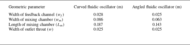
Some of the parameters in (2.28), such as $w_{\!f} , w_{m} , L_{m}$ and $w$ , can be directly obtained from the fluidic oscillator. To evaluate the general applicability of the mathematical model developed in this study, two typical fluidic oscillators were selected as benchmark cases: a curved fluidic oscillator (Ostermann et al. Reference Ostermann, Woszidlo, Nayeri and Paschereit2018) (see figure 5 a) and an angled fluidic oscillator (Seo et al. Reference Seo, Zhu and Mittal2018) (see figure 5 b). Both oscillators incorporate a mixing chamber and pair of feedback channels, and differ primarily in the use of rounded corners. Their specific geometric parameters are listed in table 1.

Figure 5.

Two typical designs of fluidic oscillators with a mixing chamber and dual-feedback channels. (a) Curved fluidic oscillator and (b) angled fluidic oscillator.

Table 1.

Geometric parameters of the curved and angled fluidic oscillators.

3.2. Determination of flow parameters

This section describes the determination of the remaining parameters in (2.28), including $b_{0} , a_{1}$ and $\sigma ^{+}$ . These parameters are related to the flow characteristics, and some must be obtained through numerical simulation or experimental measurement. To this end, the curved fluidic oscillator (figure 5 a) was simulated using the ANSYS software. Details regarding the numerical set-up, grid independence study and experimental validation are provided in Appendix A. Key flow-field data relevant to (2.28) were collected, including the jet frequency, flow velocities in the left and right feedback channels, and outlet jet sweeping angle.

Figure 6.

Area enclosed between the main jet and the mixing chamber centreline.

3.2.1. Parameter $b_{0}$

In § 2.2, we introduced a correction factor $b_{0}$ . This factor is relevant to the area enclosed between the jet and mixing chamber centreline. Taking a curved fluidic oscillator as an example, findings from both experimental literature and the numerical simulations in this study indicate that the enclosed area between the jet and the mixing chamber centreline resembles an ellipse, as shown in figure 6. Based on the elliptical area formula and (2.7), the following is obtained:

(3.1) \begin{equation} \int _{0}^{L_{m}}x(y,t)\text{d}y\approx \frac{\pi L_{m}w_{m}}{8}=\frac{b_{0}L_{m}w_{m}}{2} .\end{equation}

Here, the integral expression represents the shaded area in the figure, and $b_{0}$ is defined as the ratio of the semi-ellipse area to the area of the rectangle constructed from the length and semi-width of the mixing chamber. The above equation yields $b_{0}\approx {\pi }/{4}\approx 0.785$ . It should be noted that, analogous to the concept of mode shape in vibration mechanics, the jet ‘mode shape’ in the mixing chamber is assumed to be elliptical. In practice, this shape varies with the oscillator geometry, leading to corresponding differences in the coefficient $b_{0}$ .

3.2.2. Parameter $a_{1}$

Regarding parameter $a_{1}$ , (2.22) indicates that it is directly influenced by the relationship between $v_{\!f}/V_{j}$ and $\overline{x}$ , expressed as

(3.2) \begin{equation} \left(\frac{v_{\!f}}{V_{j}}\right)^{2}\approx a_{1}\frac{\left| \overline{x}\right| }{0.5w_{m}} .\end{equation}

Determining parameter $a_{1}$ requires knowledge of both the feedback channel velocity and relative position of the jet within the mixing chamber. However, the flow in the mixing chamber is highly complex, particularly due to the presence of separation bubbles on both sides, which poses significant challenges for directly measuring horizontal jet displacement. Therefore, for the curved fluidic oscillator, we adopted an equivalent yet simpler monitoring approach based on numerical simulation.

The sweeping angle of the outlet flow provides a representation of the jet displacement information (see figure 7), as confirmed by previous studies. By combining this with (3.2), the relationship between the deflection angle and feedback channel velocity can be summarised as follows:

(3.3) \begin{equation} \left(\frac{v_{\!f}}{V_{j}}\right)^{{\kern-1pt}2}\approx a_{1}\frac{\left| \overline{x}\right| }{0.5w_{m}}\approx a_{1}\frac{\left| \theta _{j}\right| }{\theta _{jm}} ,\end{equation}

where $\theta _{j}$ represents the sweeping angle, which is obtained by calculating the arctangent of the horizontal and vertical velocities at the outlet throat, and $\theta _{jm}$ denotes the amplitude of the sweeping angle. The outlet throat was designated as the monitoring plane for measuring the outlet sweeping angle, while a plane located 70 mm upstream of the feedback channel outlet was selected for monitoring the feedback flow velocity. The specific monitoring locations are shown in figure 7. In practice, the temporal variations in $v_{\!f}/V_{j}$ and $\theta _{j}/\theta _{jm}$ closely approximate sinusoidal curves (see figure 8). If we ignore the phase difference between the two, they can be expressed as

(3.4) \begin{equation} \left\{\!\!\begin{array}{l} \dfrac{\theta _{j}}{\theta _{jm}}\approx \sin \left(\omega _{0}t\right),\\[12pt] \dfrac{v_{\!f}}{V_{j}}\approx c_{0}\sin \left(\omega _{0}t\right),\\[12pt] \dfrac{\left| \theta _{j}\right| }{\theta _{jm}}\approx 0.5-0.5\cos \left(2\omega _{0}t\right),\\[12pt] \left(\dfrac{v_{\!f}}{V_{j}}\right)^{2}\approx {c_{0}}^{2}\left[0.5-0.5\cos \left(2\omega _{0}t\right)\right]. \end{array}\right. \end{equation}

Figure 7.

Measurement locations of $v_{\!f}$ and $\theta _{j}$ .

Figure 8.

Pulsating feedback channel velocity and outlet jet sweeping angle versus phase in a curved fluidic oscillator (numerical simulation and $V_{j}=24.4\,\text{ms}^{-1}$ ).

By combining (3.3) and (3.4), we obtain $a_{1}\approx c_{0}^{2}$ .

Based on the above analysis, the jet characteristic parameter $a_{1}$ can be determined as follows. First, the time-varying velocity in the feedback channel is monitored via numerical simulation or experiment, and the fluctuating velocity amplitude $v_{\!fm}$ is obtained through curve fitting. Subsequently, $v_{\!fm}$ is non-dimensionalised by the jet velocity $V_{j}$ and then squared to yield $a_{1}$ (i.e. ${v^{2}}_{\!fm}/{V^{2}}_{j}$ ). This study extracts the parameters based on numerical simulations; details regarding the numerical simulation set-up can be found in Appendix A. Taking the left feedback channel as representative, figure 8 presents a phase-domain plot of the pulsating flow velocity in the left feedback channel versus sweeping angle at the outlet throat for the curved fluidic oscillator at a jet velocity $V_{j}=24.4\,\text{ms}^{-1}$ , covering approximately six oscillation cycles. Following sinusoidal fitting, the fluctuating feedback velocity amplitude (green dashed line) was recognised as 0.189 (denoted as $c_{0}$ ). 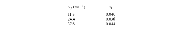Applying (3.3), the feedback force coefficient $a_{1}$ for the curved fluidic oscillator is determined as approximately 0.036. Table 2 lists the variation of $a_{1}$ at typical values of $V_{j}$ . It can be observed that $a_{1}$ remains approximately constant ( $a_{1}\approx 0.04$ ) with changes in $V_{j}$ , indicating that $a_{1}$ is not largely affected by the jet velocity but may be determined by geometry. Therefore, for the curved fluidic oscillator, we set $a_{1}\approx 0.04$ . This study also examines the value of $a_{1}$ in the angled fluidic oscillator (figure 5 b). Data are sourced from Seo et al. (Reference Seo, Zhu and Mittal2018), where the Reynolds number is approximately 5000 and the flow is incompressible. Based on the pulsating velocity data from the feedback channels, the oscillation amplitude of $v_{\!f}/V_{j}$ is measured as approximately 0.2 (i.e. $c_{0}\approx 0.2$ ). Thus, $a_{1}\approx c_{0}^{2}\approx 0.04$ , which is very close to the value of $a_{1}$ in the adopted curved fluidic oscillator.

Table 2.

Variation of parameter $a_{1}$ with jet velocity for the curved fluidic oscillator.

3.2.3. Parameter $\sigma ^{+}$

Equation (2.28) indicates that the parameter $\sigma ^{+}$ is related to the wall attachment of the jet in the mixing chamber when no feedback channel is present, and therefore requires time-domain data of $\overline{x}$ obtained from a fluidic oscillator without feedback channels. Building upon the adopted curved fluidic oscillator, the present numerical simulation deliberately decouples the feedback channels from the fluidic oscillator. Figure 9 shows the precise location of this decoupling, where the inlets and outlets of the feedback channels are defined as wall boundaries. Without feedback, the jet attaches itself to one mixing chamber wall through the Coanda effect, exhibiting no oscillation. Growth rate data were acquired during the jet development phase. At the outlet throat, variations in the jet sweeping angle $\theta _{j}/\theta _{jm}$ serve as a proxy for changes in $\overline{x}/(0.5w_{m})$ , as expressed in (3.3).

Figure 9.

Curved fluidic oscillator without feedback channels.

Figure 10.

Instantaneous velocity field in a curved fluidic oscillator without feedback channels ( $V_{j}=24.4\,\text{ms}^{-1}$ ).

Figure 11.

Coanda attachment behaviour in a curved fluidic oscillator without feedback channels across different jet velocities.

The sweeping angle growth rate is determined by fitting the data using (2.24) in dimensionless coordinates. Figure 10 displays instantaneous velocity contours at three specific time instances ( $V_{j}=24.4\,\text{ms}^{-1}$ ). As observed in figure 10, the main jet gradually attaches to the right wall of the mixing chamber due to the Coanda effect, rapidly reaching its maximum sweeping angle. In the absence of a feedback mechanism, this attached state remains relatively stable and will not transition unless perturbed; for instance, by the inherent Kelvin–Helmholtz (K–H) instability of the jet. Figure 11 illustrates the development of wall-attached jets in a curved fluidic oscillator without feedback channels at three different jet velocities. Since no artificial perturbations were introduced in our simulations, the attachment process evolved freely. As a result, the inherent randomness in the initial amplitude of small-scale oscillations – caused by the K–H instability in the developing jet – led to variations in the timing of attachment onset. To consistently characterise the growth rate of the attachment effect, this study defines time zero (t = 0) as the moment when the sweeping angle $\theta _{j}/\theta _{jm}\approx 0.2$ . 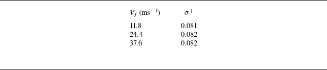The amplitude data points are fitted using (2.24), with the fitting results shown in figure 11. It can be observed that after non-dimensionalising time, the jet growth patterns under the three velocities are similar. Table 3 lists the values of $\sigma ^{+}$ at the three jet velocities; the results indicate that $\sigma ^{+}$ remains nearly constant. Therefore, within the incompressible range considered in this study, a unified value of $\sigma ^{+}\approx 0.08$ was adopted for subsequent calculations.

Table 3.

Variation of $\sigma ^{+}$ with jet velocity in the curved fluidic oscillator without feedback channels.

Based on the determination of jet characteristic parameters in §§ 3.2.1–3.2.3, it is found that under conditions of fixed geometry and incompressible flow, the three characteristic parameters of the model remain nearly constant. However, in practice, these parameters may vary with changes in geometric configuration or under compressible conditions. For example, under compressible flow conditions, the parameters $a_{1}$ may become a function of $V_{j}$ . For different geometric parameters, their variation may lead to changes in model parameters or even oscillation modes. Specifically, the parameter $a_{1}$ is related to the flow distribution ratio between the mixing chamber and the feedback channels. It may be influenced by the width and length of the mixing chamber, as well as the angle and shape of its upper wall. The parameter $b_{0}$ is related to the shape of the jet within the mixing chamber and could be affected by the width, length and wall profile of the mixing chamber. Meanwhile, the parameter $\sigma ^{+}$ , which is closely related to the Coanda effect term, may be influenced by the width of the inlet throat, the width, length and shape of the mixing chamber. The effects of these parameters need to be elucidated via systematic and extensive numerical and experimental work.

4.1. The invariance of St in relation to proportional scaling

The approximate expression for the St is given by (2.33)

(4.1) \begin{equation} St\approx \frac{1}{\pi }\sqrt{\frac{a_{1}w_{\!f}w}{b_{0}L_{m}w_{m}}} ,\end{equation}

where, $a_{1}$ characterises the strength of feedback effect or the $v_{\!f}/V_{j}$ ratio, $b_{0}$ represents the shape of the jet within the mixing chamber and other parameters characterise the fluidic oscillator geometry. As demonstrated in §§ 3.2.1 and 3.2.2, parameters $a_{1}$ and $b_{0}$ are approximately constant over a range of jet velocities for a fixed fluidic oscillator geometry within the incompressible flow regime. Since $a_{1}$ and $b_{0}$ are dimensionless ratios determined by the geometry of the oscillator, it follows that they will also remain approximately constant – effectively scale invariant – when the oscillator is geometrically scaled, provided the flow remains incompressible and the Reynolds number does not change significantly. Furthermore, $({w_{\!f}w}/{L_{m}w_{m}})$ remains unchanged under geometric scaling of the fluidic oscillator. Hence, St remains essentially constant during geometric scaling of the fluidic oscillator. This behaviour is consistent with observations reported in the literature (Schmidt et al. Reference Schmidt, Woszidlo, Nayeri and Paschereit2017). It should be noted that (2.28) is an approximate expression. The compressibility effects, influence of the Reynolds number, higher-order terms such as $a_{2}$ and $a_{3}$ in (2.20), and the contribution of $\sigma$ in (2.30) may cause the actual St to vary slightly during geometric scaling.

4.2. Theoretical prediction of St

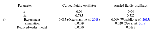
Based on the parameter extraction detailed in §§ 3.1 and 3.2, this section provides a theoretical prediction of the St for both curved and angled fluidic oscillator designs. Table 4 presents the predicted St values of the ROM (using (4.1)) for the two typical fluidic oscillators (as illustrated in figures 5(a) and 5(b)). Despite being derived from a set of simplifying assumptions and approximations, the ROM showed good agreement with experimental measurements. This validates that the ROM captures the primary operating mechanism of the fluidic oscillator.

Table 4.

Comparison of model-predicted, simulated and experimental St for two fluidic oscillator designs.

4.3. Relationship between sweeping frequency and jet velocity

According to (2.31) and (2.32)

(4.2) \begin{equation} f_{0}\approx \frac{1}{\pi w}\sqrt{\frac{a_{1}w_{\!f}w}{b_{0}L_{m}w_{m}}}V_{j}=\frac{St}{w}V_{j} .\end{equation}

Therefore, in the proposed ROM, the sweeping frequency of the fluidic oscillator was proportional to the jet velocity. For the curved fluidic oscillator, this relation was compared with experimental data from the literature (Ostermann et al. Reference Ostermann, Woszidlo, Nayeri and Paschereit2018) and numerical simulations, as shown in figure 12. Specifically, we conducted numerical simulations of the curved fluidic oscillator at three distinct outlet throat velocities, from which the corresponding oscillation frequencies were obtained via fast Fourier transform analysis. As shown in figure 12, the frequency trends from all three methods showed close agreement. This result demonstrates that the proposed ROM accurately captures the dependence of the oscillation frequency on the jet velocity for the curved fluidic oscillator in the incompressible regime.

Figure 12.

A comparison among model predictions, numerical simulations and experimental results for the relationship between oscillation frequency and jet velocity (for the curved fluidic oscillator).

Figure 13.

Time-domain curves of model predicted versus the numerically simulated sweeping angle (for the curved fluidic oscillator, and $V_{j}=24.4\,\text{ms}^{-1}$ ).

4.4. Time-domain curves of the sweeping angle

This section discusses the effectiveness in simulating the evolution of the sweeping angle of the curved fluidic oscillator. Using MATLAB, the time-domain curve for the model predicted sweeping angle $\theta _{j}$ was simulated and compared with the numerically simulated curve using computation fluid dynamics, as shown in figure 13.

The ROM simulation was conducted with a time step and duration of 0.001 and 0.5 s, respectively. The initial conditions were set to $\overline{x}(0)$ = 0 and $\dot{\overline{x}}(0)$ = 0.5. The figure demonstrates that the model accurately captures the evolution of the sweeping angle, including its development phase. Nevertheless, during the first oscillation cycle between t = 0 and t = 0.05 s, the model predicts an earlier initial growth of the sweeping angle compared with the numerical simulations. This occurs because the monitoring plane in the numerical simulation is located at the outlet throat, and the jet downstream can be approximated as a free jet. During the initial development stage, the jet is more significantly influenced by K–H instability, which results in relatively higher-frequency fluctuations near the outlet. In the fully developed stage, however, the sweeping motion at the outlet is primarily governed by the wall-attachment and feedback mechanism in the mixing chamber, which operates at a lower characteristic frequency, while the influence of K–H instability becomes less pronounced. Since the theoretical model in this study only considers the wall-attachment and feedback mechanism, a discrepancy appears between the model predictions and the numerical results during the initial development stage, where K–H instability dominates. Once the sweeping jet becomes fully developed, however, its sweeping behaviour is governed primarily by the wall-attachment and feedback mechanism, with minimal influence from K–H instability. This leads to good agreement between the numerical and modelled results in the fully developed state (as shown in figure 13).

It should be noted that K–H instability is an inherent characteristic of free jets. In practice, the K–H waves during the initial stage provide both the initial perturbation amplitude and velocity for the model. These factors influence the time required for the sweeping angle–time curve to reach saturation, as well as the phase in the fully developed state. Indeed, in repeated runs of experiments or simulations with identical configurations, the initial development stage may also vary due to differences in initial disturbances.

Based on these observations, it was concluded that the model demonstrates significant accuracy in predicting the temporal evolution of the sweeping angle, except for the initial development stage dominated by the K–H instability.

4.5. The influence of geometric parameter variations and limitations of the model

In the previous section, we examined the predictive performance of the reduced-order model for fluidic oscillators with fixed geometries. In this section, we investigate whether the model maintains its predictive capability when typical geometric parameters are altered, with a discussion of its limitations.

Figure 14 illustrates the predictive performance of the reduced-order model for the characteristics of angled fluidic oscillators with varying feedback channel lengths ( $L_{\!f}$ ), width ( $w_{\!f}$ ) and mixing chamber lengths ( $L_{m}$ ). The comparative numerical data were obtained from Seo et al. (Reference Seo, Zhu and Mittal2018) and the present study. The geometric parameters under investigation – specifically their impact on St – were all normalised by the outlet throat width ( $w$ ).

Figure 14.

Effect of typical geometric parameters on St. (a) Feedback channel length $L_{\!f}$ , (b) feedback channel width $w_{\!f}$ and (c) mixing chamber length $L_{m}$ .

In figures 14(a) and 14(b), when the feedback channel dimensions (length $L_{\!f}$ and width $w_{\!f}$ ) do not vary substantially and the mixing chamber geometry is held constant, the pressure difference across the feedback channel remains largely unchanged. Consequently, the velocity ratio $v_{\!f}/V_{j}$ remains approximately constant, leading to only a minor variation in the parameter $a_{1}$ . Since the mixing chamber is unchanged, the parameters describing the jet shape and the wall-attachment effect, $b_{0}$ and $\sigma ^{+}$ , should also remain largely invariant. With $a_{1}$ and $b_{0}$ held constant under these conditions, the predictions of the reduced-order model show good agreement with the numerical simulation results, as demonstrated in figures 14(a) and 14(b).

Regarding the feedback channel length ( $L_{\!f}$ ), since the expression for St proposed in this paper (4.1) does not incorporate this parameter, the model-predicted St remains constant. This aligns well with the findings from Seo et al. (Reference Seo, Zhu and Mittal2018), as shown in figure 14(a). It should be noted, however, that when $L_{\!f}$ becomes excessively long, the internal flow state of the fluidic oscillator tends to become steady. In such cases, St is no longer governed by the attachment and feedback mechanisms but by the K–H instability, resulting in a significantly higher value (Bergadà et al. Reference Bergadà, Baghaei, Prakash and Mellibovsky2021; Gui, Lu & Lu Reference Gui, Lu, Yan and Lu2026). The current model fails to predict this phenomenon, highlighting its inherent limitation. This limitation arises primarily from two unmodeled effects associated with the feedback channels. First, an excessively long or narrow feedback channel introduces significant flow losses within the channel. Second, a long feedback channel necessitates considering the propagation time of pressure waves, thereby introducing compressibility effects dependent on the speed of sound. Both the internal flow loss and fluid compressibility within the feedback channels are neglected in the present reduced-order model. Moreover, under high-speed conditions where compressibility must be considered, the development of pressure waves in the feedback channels (Bergadà et al. Reference Bergadà, Baghaei, Prakash and Mellibovsky2021) means that the inlet and outlet velocities are no longer approximately equal, deviating from the assumption made in the present model. If compressibility is considered, the propagation time of pressure waves within the feedback channel increases the oscillation period, leading to a corresponding decrease in the oscillation frequency (Yan et al. Reference Yan, Lu, Yang, Deng and Lu2023). Regarding the feedback channel width ( $w_{\!f}$ ), as shown in figure 14(b), the predicted St from the model agrees well with the numerical simulation results, both of which decrease as the channel width is reduced.

Regarding the mixing chamber length ( $L_{m}$ ), its increase could theoretically alter the parameters $a_{1}$ , $b_{0}$ and $\sigma ^{+}$ . We referred to the numerical simulation data from Seo et al. (Reference Seo, Zhu and Mittal2018), which indicated that moderate variations in $L_{m}$ lead to negligible changes in both the pulsating velocity within the feedback channel and the jet shape within the mixing chamber. Consequently, the parameters $a_{1}$ and $b_{0}$ are treated as constants in the model. As shown in figure 14(c), the reduced-order model predicts the decreasing trend of St with increasing mixing chamber length and this trend is consistent with the numerical results from Seo et al. (Reference Seo, Zhu and Mittal2018). However, for larger mixing chamber lengths, an apparent discrepancy emerges between the model predictions and the numerical results. We attribute this error to two possible factors. First, as indicated by Seo et al. (Reference Seo, Zhu and Mittal2018), a phase difference exists between the jet at the inlet and outlet of the mixing chamber. This phase difference introduces an additional feedback delay, which reduces the oscillation frequency and becomes more pronounced with increasing chamber length. Our model neglects this effect by approximating the jet oscillation within the chamber as a standing wave (analogous to a mode shape in vibration). Second, Seo et al. (Reference Seo, Zhu and Mittal2018) also indicate that the influence of the growth and decay of separation bubbles within the chamber becomes more dominant as its length increases. The evolution of these bubbles may effectively increase the inertia of jet oscillation, thereby lowering its oscillation frequency. Since our reduced-order model primarily considers the feedback and jet-attachment mechanisms, it does not account for this extra inertia contributed by the separation bubbles, leading to the observed error.

Based on figure 14, it can be observed that for the angled fluidic oscillator, with the parameters in the ranges $8\leq L_{\!f}/w\leq 12 , 0.5\leq w_{\!f}/w\leq 1$ , and $5.75\leq L_{m}/w\leq 6.25$ , the predictions from the St expression agree with the numerical simulation results to within 10 %, demonstrating a satisfactory level of accuracy. Owing to the limited numerical data currently available, the actual parameter range over which the St expression yields reliable predictions is likely broader than that reported above. Extending this range warrants further investigation with more extensive data. In § 4.2, when predicting the St of two typical fluidic oscillators, the values $a_{1}$ = 0.04 and $b_{0}$ = 0.785 were adopted and found to yield satisfactory predictive performance. Furthermore, throughout § 4.5, these same parameter values ( $a_{1}$ = 0.04, $b_{0}$ = 0.785) were retained while other geometric parameters were varied, and the predictions remained consistently reliable. On this basis, it is recommended that when applying the proposed reduced-order model to predict the characteristics of other fluidic oscillator configurations, $a_{1}$ and $b_{0}$ be initially set to these typical values of 0.04 and 0.785, respectively, and subsequently fine-tuned in accordance with results from numerical simulations.

Although the current model demonstrates predictive accuracy in some cases, it still has notable limitations. It performs well in predicting the behaviour of well-designed fluidic oscillators – where the feedback and Coanda effects are dominant and function properly – operating under incompressible flow conditions. However, the model’s predictive accuracy may decrease in two main cases. The first case occurs when a single geometric parameter changes sufficiently to alter the oscillator’s operational mechanism. The second case occurs when the underlying model assumptions or approximations are no longer valid – for example, when compressibility can no longer be ignored or when viscous losses in the feedback channels become significant. Nevertheless, the current model successfully captures key dominant mechanisms, thereby providing a theoretical framework for subsequent modification. To develop a more precise and broadly applicable model, future work could refine the present framework by incorporating effects such as compressibility, flow losses within the feedback channels, the phase difference of the jet at different positions in the mixing chamber, and the additional inertia arising from the evolution of separation bubbles.