1 Introduction
Parametric geometry of numbers is a new theory, recently created by Schmidt and Summerer [Reference Schmidt and Summerer12, Reference Schmidt and Summerer13], which unifies and simplifies many aspects of classical Diophantine approximation, providing a handle on problems which previously seemed out of reach (see also [Reference Schmidt11]). Our goal is to transpose this theory to fields of rational functions in one variable and to analyze in that context the problem of simultaneous approximation to exponential functions.
Expressed in the setting of [Reference Roy10], the theory deals with a general family of convex bodies of the form
 $$\begin{eqnarray}{\mathcal{C}}_{\mathbf{u}}(\text{e}^{q})=\{\mathbf{x}\in \mathbb{R}^{n};\Vert \mathbf{x}\Vert \leqslant 1\text{ and }|\mathbf{u}\cdot \mathbf{x}|\leqslant \text{e}^{-q}\}\quad (q\geqslant 0),\end{eqnarray}$$
where the norm is the Euclidean norm,
 $\mathbf{u}$
is a fixed unit vector in
 $\mathbb{R}^{n}$
, and
 $\mathbf{u}\cdot \mathbf{x}$
denotes the scalar product of
 $\mathbf{u}$
and
 $\mathbf{x}$
. For each
 $i=1,\ldots ,n$
, let
 $L_{\mathbf{u},i}(q)$
be the logarithm of the
 $i$
th minimum of
 ${\mathcal{C}}_{\mathbf{u}}(\text{e}^{q})$
with respect to
 $\mathbb{Z}^{n}$
, that is the minimum of all
 $t\in \mathbb{R}$
such that
 $\text{e}^{t}{\mathcal{C}}_{\mathbf{u}}(\text{e}^{q})$
contains at least
 $i$
linearly independent elements of
 $\mathbb{Z}^{n}$
. Equivalently, this is the smallest
 $t$
for which the solutions
 $\mathbf{x}$
in
 $\mathbb{Z}^{n}$
of
 $$\begin{eqnarray}\Vert \mathbf{x}\Vert \leqslant \text{e}^{t}\quad \text{and}\quad |\mathbf{u}\cdot \mathbf{x}|\leqslant \text{e}^{t-q}\end{eqnarray}$$
span a subspace of
 $\mathbb{Q}^{n}$
of dimension at least
 $i$
. Define
 $$\begin{eqnarray}\begin{array}{@{}rl@{}}\mathbf{L}_{\mathbf{u}}:[0,\infty )\ & \longrightarrow \mathbb{R}^{n}\\ q\ & \longmapsto (L_{\mathbf{u},1}(q),\ldots ,L_{\mathbf{u},n}(q)).\end{array}\end{eqnarray}$$
Although the behavior of the maps
 $\mathbf{L}_{\mathbf{u}}$
may be complicated (even for
 $n=2$
, see [Reference Keita5]), it happens that, modulo the additive group of bounded functions from
 $[0,\infty )$
to
 $\mathbb{R}^{n}$
, their classes are the same as those of simpler functions called
 $n$
-systems, defined as follows.
An
 $n$
-system on
 $[0,\infty )$
is a map
 $\mathbf{P}=(P_{1},\ldots ,P_{n}):[0,\infty )\rightarrow \mathbb{R}^{n}$
with the property that, for each
 $q\geqslant 0$
, the following hold.
-
(S1) We have
 $0\leqslant P_{1}(q)\leqslant \cdots \leqslant P_{n}(q)$
and
$P_{1}(q)+\cdots +P_{n}(q)=q$
.
-
(S2) There exist
$\unicode[STIX]{x1D716}>0$
and integers
$k,\ell \in \{1,\ldots ,n\}$
such that where
$$\begin{eqnarray}\mathbf{P}(t)=\left\{\begin{array}{@{}ll@{}}\mathbf{P}(q)+(t-q)\mathbf{e}_{\ell }\quad & \text{when }\max \{0,q-\unicode[STIX]{x1D716}\}\leqslant t\leqslant q,\\ \mathbf{P}(q)+(t-q)\mathbf{e}_{k}\quad & \text{when }q\leqslant t\leqslant q+\unicode[STIX]{x1D716},\end{array}\right.\end{eqnarray}$$
$\mathbf{e}_{1}=(1,0,\ldots ,0),\ldots ,\mathbf{e}_{n}=(0,\ldots ,0,1)$
.
-
(S3) If
$q>0$
and if the integers
$k$
and
$\ell$
from (S2) satisfy
$k>\ell$
, then we have
$P_{\ell }(q)=\cdots =P_{k}(q)$
.





By [Reference Roy10, Theorems 8.1 and 8.2], there is an explicit constant
 $C(n)$
, depending only on
 $n$
, such that, for each unit vector
 $\mathbf{u}\in \mathbb{R}^{n}$
, there exists an
 $n$
-system
 $\mathbf{P}$
on
 $[0,\infty )$
such that
 $\Vert \mathbf{L}_{\mathbf{u}}(q)-\mathbf{P}(q)\Vert \leqslant C(n)$
for each
 $q\geqslant 0$
, and conversely, for each
 $n$
-system
 $\mathbf{P}$
on
 $[0,\infty )$
, there exists a unit vector
 $\mathbf{u}\in \mathbb{R}^{n}$
with the same property.
Instead of
 $\mathbb{Z}$
, we work here with a ring of polynomials
 $A=F[T]$
in one variable
 $T$
over an arbitrary field
 $F$
. We denote by
 $K=F(T)$
its field of quotients equipped with the absolute value given by
 $$\begin{eqnarray}|f/g|=\exp (\deg (f)-\deg (g))\end{eqnarray}$$
for any
 $f,g\in A$
with
 $g\neq 0$
(using the convention that
 $\deg (0)=-\infty$
and
 $\exp (-\infty )=0$
). The role of
 $\mathbb{R}$
is now played by the completion
 $K_{\infty }=F((1/T))$
of
 $K$
with respect to that absolute value. The extension of this absolute value to
 $K_{\infty }$
is also denoted
 $|~|$
. We fix an integer
 $n\geqslant 2$
and still denote by
 $(\mathbf{e}_{1},\ldots ,\mathbf{e}_{n})$
the canonical basis of
 $K_{\infty }^{n}$
. We endow
 $K_{\infty }^{n}$
with the maximum norm
 $$\begin{eqnarray}\Vert \mathbf{x}\Vert =\max \{|x_{1}|,\ldots ,|x_{n}|\}\quad \text{if }\mathbf{x}=(x_{1},\ldots ,x_{n}).\end{eqnarray}$$
We also use the non-degenerate bilinear form on
 $K_{\infty }^{n}\times K_{\infty }^{n}$
mapping a pair
 $(\mathbf{x},\mathbf{y})$
to
 $$\begin{eqnarray}\mathbf{x}\cdot \mathbf{y}=x_{1}y_{1}+\cdots +x_{n}y_{n}\quad \text{if }\mathbf{x}=(x_{1},\ldots ,x_{n})~\text{and}~\mathbf{y}=(y_{1},\ldots ,y_{n}).\end{eqnarray}$$
This identifies
 $K_{\infty }^{n}$
with its dual isometrically in the sense that
 $$\begin{eqnarray}\Vert \mathbf{x}\Vert =\max \{|\mathbf{x}\cdot \mathbf{y}|;\mathbf{y}\in K_{\infty }^{n}\text{ and }\Vert \mathbf{y}\Vert \leqslant 1\}\end{eqnarray}$$
for any
 $\mathbf{x}\in K_{\infty }^{n}$
. For a given
 $\mathbf{u}\in K_{\infty }^{n}$
of norm 1, for each
 $i=1,\ldots ,n$
and each
 $q\geqslant 0$
, we define
 $L_{\mathbf{u},i}(q)$
to be the minimum of all
 $t\geqslant 0$
for which the solutions
 $\mathbf{x}$
in
 $A^{n}$
of the inequalities (1.1), interpreted in
 $K_{\infty }^{n}$
, span a subspace of
 $K^{n}$
of dimension at least
 $i$
. This minimum exists as we may restrict to values of
 $t$
in
 $\mathbb{Z}$
or in
 $q+\mathbb{Z}$
. Then we form a map
 $\mathbf{L}_{\mathbf{u}}:[0,\infty )\rightarrow \mathbb{R}^{n}$
as in (1.2) above. Our first main result reads as follows.
Theorem A. The set of maps
 $\mathbf{L}_{\mathbf{u}}$
where
 $\mathbf{u}$
runs through the elements of
 $K_{\infty }^{n}$
of norm
 $1$
is the same as the set of
 $n$
-systems
 $\mathbf{P}$
on
 $[0,\infty )$
with
 $\mathbf{P}(q)\in \mathbb{Z}^{n}$
for each integer
 $q\geqslant 0$
.
As we will see in the next section, when
 $q$
belongs to the set
 $\mathbb{N}=\{0,1,2,\ldots \}$
of non-negative integers, the numbers
 $L_{\mathbf{u},1}(q),\ldots ,L_{\mathbf{u},n}(q)$
are the logarithms of the successive minima of a convex body
 ${\mathcal{C}}_{\mathbf{u}}(\text{e}^{q})$
of
 $K_{\infty }^{n}$
with respect to
 $A^{n}$
, as defined by Mahler in [Reference Mahler7]. However, in terms of the inequalities (1.1), these functions naturally extend to all real numbers
 $q\geqslant 0$
.
The proof of Theorem A is similar to that of the previously mentioned result over
 $\mathbb{Q}$
, but much simpler in good part because, as Mahler proved in the same paper [Reference Mahler7], the analog of Minkowski’s second convex body theorem holds with an equality in that setting. There is also the fact that the group of isometries of
 $K_{\infty }^{n}$
is an open set in
 $\text{GL}_{n}(K_{\infty })$
, and thus in that sense much larger than the orthogonal group of
 $\mathbb{R}^{n}$
. In §§2 and 3, we give a complete proof of Theorem A following [Reference Roy10]. The fact that each map
 $\mathbf{L}_{\mathbf{u}}$
is an
 $n$
-system is an adaptation of the argument of Schmidt and Summerer in [Reference Schmidt and Summerer13, §2]. In §4, we also connect the maps
 $\mathbf{L}_{\mathbf{u}}$
with the analogue of those considered by these authors in [Reference Schmidt and Summerer13].
Because of the condition (S1), an
 $n$
-system
 $\mathbf{P}=(P_{1},\ldots ,P_{n})$
on
 $[0,\infty )$
mapping
 $\mathbb{N}$
to
 $\mathbb{N}^{n}$
satisfies
 $$\begin{eqnarray}P_{1}(q)\leqslant \biggl\lfloor\frac{q}{n}\biggr\rfloor\leqslant \lceil \frac{q}{n}\rceil \leqslant P_{n}(q)\quad \text{for each }q\in \mathbb{N}.\end{eqnarray}$$
It happens that there is exactly one such
 $n$
-system for which
 $$\begin{eqnarray}P_{1}(q)=\biggl\lfloor\frac{q}{n}\biggr\rfloor\quad \text{and}\quad P_{n}(q)=\lceil \frac{q}{n}\rceil \quad \text{for each }q\in \mathbb{N}.\end{eqnarray}$$
When
 $q\equiv 0~\text{mod}~n$
, such a system necessarily has
 $P_{1}(q)=\cdots =P_{n}(q)=q/n$
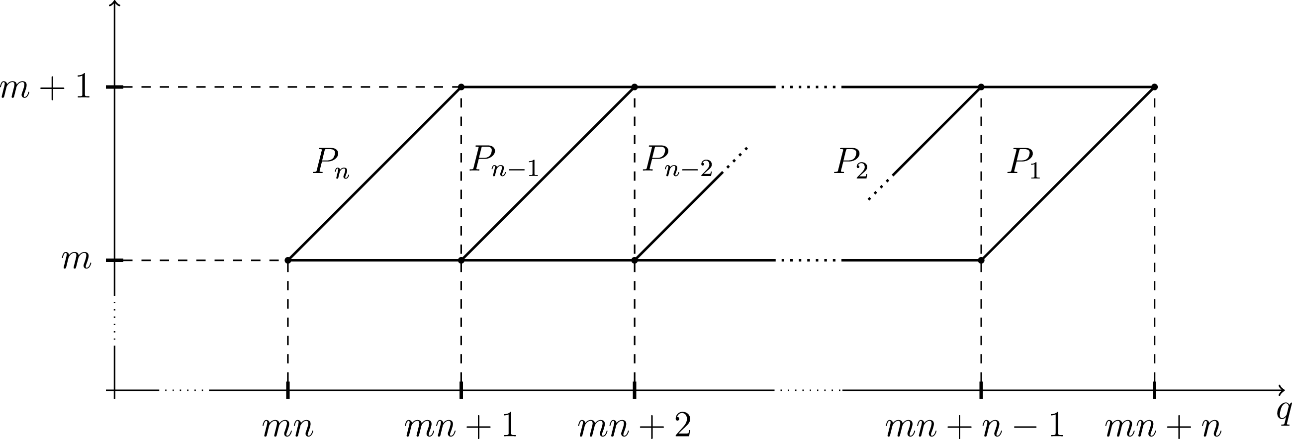
. Figure 1 shows the union of the graphs of
 $P_{1},\ldots ,P_{n}$
over an interval of the form
 $[mn,(m+1)n]$
with
 $m\in \mathbb{N}$
. Over such an interval, the
 $i$
th component
 $P_{i}$
of
 $\mathbf{P}$
is constant equal to
 $m$
on
 $[mn,mn+n-i]$
, then increases with slope 1 on
 $[mn+n-i,mn+n-i+1]$
and finally is constant equal to
 $m+1$
on
 $[mn+n-i+1,mn+n]$
.
The combined graph of the
 $n$
-system satisfying (1.4).

One can also characterize that system as the unique one which satisfies
 $P_{n}(q)-P_{1}(q)\leqslant 1$
for each
 $q\geqslant 0$
. Our second main result is the following.
Theorem B. Suppose that
 $F$
has characteristic zero. Let
 $\unicode[STIX]{x1D714}_{1},\ldots ,\unicode[STIX]{x1D714}_{n}$
be distinct elements of
 $F$
, and let
 $$\begin{eqnarray}\mathbf{u}=(\text{e}^{\unicode[STIX]{x1D714}_{1}/T},\ldots ,\text{e}^{\unicode[STIX]{x1D714}_{n}/T})\quad \text{where }\text{e}^{\unicode[STIX]{x1D714}/T}=\mathop{\sum }_{j=0}^{\infty }\frac{\unicode[STIX]{x1D714}^{j}}{j!}T^{-j}\in F[[1/T]]\quad (\unicode[STIX]{x1D714}\in F).\end{eqnarray}$$
Then, we have
 $\Vert \mathbf{u}\Vert =1$
and the
 $n$
-system
 $\mathbf{P}=\mathbf{L}_{\mathbf{u}}$
is characterized by the property (1.4).
As we will show in §5, this result in fact extends to all perfect systems of series in the sense of Mahler and Jager [Reference Jager4, Reference Mahler9].
In 1964, Baker showed that, in the notation of Theorem B, the
 $n$
-tuple
 $(\text{e}^{\unicode[STIX]{x1D714}_{1}/T},\ldots ,\text{e}^{\unicode[STIX]{x1D714}_{n}/T})$
provides a counterexample to the analogue in
 $\mathbb{C}((1/T))$
of a conjecture of Littlewood. In §6, we generalize this result to several places of
 $\mathbb{C}(T)$
.
2 Constraints on the successive minima
In this section, we prove that the maps
 $\mathbf{L}_{\mathbf{u}}$
which appear in Theorem A are
 $n$
-systems. The argument is based on the ideas of Schmidt and Summerer in [Reference Schmidt and Summerer13], but follows the presentation in [Reference Roy10, §2].
2.1 Convex bodies
We fix an integer
 $n\geqslant 1$
and denote by
 $$\begin{eqnarray}{\mathcal{O}}_{\infty }=\{x\in K_{\infty };|x|\leqslant 1\}=F[[1/T]]\end{eqnarray}$$
the ring of integers of
 $K_{\infty }$
. A convex body of
 $K_{\infty }^{n}$
is simply a free sub-
 ${\mathcal{O}}_{\infty }$
-module of
 $K_{\infty }^{n}$
of rank
 $n$
. This seemingly narrow notion, the analog of a parallelotope, is explained by Mahler in [Reference Mahler7]. For example, the unit ball
 ${\mathcal{O}}_{\infty }^{n}$
of
 $K_{\infty }^{n}$
for the maximum norm is a convex body.
Let
 ${\mathcal{C}}$
be an arbitrary convex body of
 $K_{\infty }^{n}$
. Its volume
 $\text{vol}({\mathcal{C}})$
is defined as the common value
 $|\text{det}(\unicode[STIX]{x1D713})|$
attached to all
 $K_{\infty }$
-linear automorphisms
 $\unicode[STIX]{x1D713}$
of
 $K_{\infty }^{n}$
for which
 $\unicode[STIX]{x1D713}({\mathcal{O}}_{\infty }^{n})={\mathcal{C}}$
. For each
 $i=1,\ldots ,n$
, the
 $i$
th minimum of
 ${\mathcal{C}}$
(with respect to
 $A^{n}$
) is defined as the smallest number
 $|\unicode[STIX]{x1D70C}|$
where
 $\unicode[STIX]{x1D70C}$
runs through the elements of
 $K_{\infty }^{\times }$
for which the dilated convex body
 $$\begin{eqnarray}\unicode[STIX]{x1D70C}{\mathcal{C}}=\{\unicode[STIX]{x1D70C}\mathbf{x};\mathbf{x}\in {\mathcal{C}}\}\end{eqnarray}$$
contains at least
 $i$
linearly independent elements of
 $A^{n}$
. Since
 $\unicode[STIX]{x1D70C}{\mathcal{C}}$
depends only on the class
 $\unicode[STIX]{x1D70C}{\mathcal{O}}_{\infty }^{\times }$
in
 $K_{\infty }^{\times }/{\mathcal{O}}_{\infty }^{\times }$
, we may restrict to elements of the form
 $\unicode[STIX]{x1D70C}=T^{a}$
with
 $a\in \mathbb{Z}$
. In this context, Mahler’s extension of Minkowski’s convex body theorem in [Reference Mahler7, §9], reads as follows (compare with the version proved by Thunder over an arbitrary function field in [Reference Thunder14]).
Theorem 2.1. For
 $i=1,\ldots ,n$
, let
 $\unicode[STIX]{x1D706}_{i}=\text{e}^{\unicode[STIX]{x1D707}_{i}}$
be the
 $i$
th minimum of
 ${\mathcal{C}}$
. Then we have
 $$\begin{eqnarray}\unicode[STIX]{x1D706}_{1}\cdots \unicode[STIX]{x1D706}_{n}\text{vol}({\mathcal{C}})=1.\end{eqnarray}$$
Moreover, there exists a basis
 $(\mathbf{x}_{1},\ldots ,\mathbf{x}_{n})$
of
 $A^{n}$
over
 $A$
such that
 $\mathbf{x}_{i}\in T^{\unicode[STIX]{x1D707}_{i}}{\mathcal{C}}$
for
 $i=1,\ldots ,n$
.
The last property is expressed by saying that
 $\mathbf{x}_{1},\ldots ,\mathbf{x}_{n}$
realize the successive minima
 $\unicode[STIX]{x1D706}_{1}\leqslant \ldots \leqslant \unicode[STIX]{x1D706}_{n}$
of
 ${\mathcal{C}}$
.
Mahler defines the dual or polar body to
 ${\mathcal{C}}$
by
 $$\begin{eqnarray}{\mathcal{C}}^{\ast }=\{\mathbf{y}\in K_{\infty }^{n};|\mathbf{x}\cdot \mathbf{y}|\leqslant 1\text{ for all }\mathbf{x}\in {\mathcal{C}}\}.\end{eqnarray}$$
This is a convex body of
 $K_{\infty }^{n}$
with
 $\text{vol}({\mathcal{C}}^{\ast })=\text{vol}({\mathcal{C}})^{-1}$
. On the algebraic counterpart, for any basis
 $(\mathbf{x}_{1},\ldots ,\mathbf{x}_{n})$
of
 $A^{n}$
, there is a dual basis
 $(\mathbf{x}_{1}^{\ast },\ldots ,\mathbf{x}_{n}^{\ast })$
of
 $A^{n}$
characterized by
 $\mathbf{x}_{i}^{\ast }\cdot \mathbf{x}_{j}=\unicode[STIX]{x1D6FF}_{i,j}$
 $(1\leqslant i\leqslant j\leqslant n)$
. In [Reference Mahler7, §10], Mahler shows the following.
Theorem 2.2. In the notation of the previous theorem, the successive minima of
 ${\mathcal{C}}^{\ast }$
are
 $\unicode[STIX]{x1D706}_{n}^{-1}\leqslant \cdots \leqslant \unicode[STIX]{x1D706}_{1}^{-1}$
, realized by the elements of the dual basis to
 $(\mathbf{x}_{1},\ldots ,\mathbf{x}_{n})$
listed in reverse order
 $\mathbf{x}_{n}^{\ast },\ldots ,\mathbf{x}_{1}^{\ast }$
.
Mahler’s original theory of compound bodies (over
 $\mathbb{R}$
) also extends to the present setting. To state the result, fix
 $m\in \{1,\ldots ,n\}$
and put
 $N=\binom{n}{m}$
. We identify
 $\bigwedge ^{m}K_{\infty }^{n}$
with
 $K_{\infty }^{N}$
via a linear map sending the
 $N$
products
 $\mathbf{e}_{i_{1}}\wedge \cdots \wedge \mathbf{e}_{i_{m}}$
with
 $1\leqslant i_{1}<\cdots <i_{m}\leqslant n$
to the elements of the canonical basis of
 $K_{\infty }^{N}$
in some order. Then, the sub-
 $A$
-module
 $\bigwedge ^{m}A^{n}$
of
 $\bigwedge ^{m}K_{\infty }^{n}$
generated by the products
 $\mathbf{v}_{1}\wedge \cdots \wedge \mathbf{v}_{m}$
with
 $\mathbf{v}_{1},\ldots ,\mathbf{v}_{m}\in A^{n}$
is identified with
 $A^{N}$
. The
 $m$
th compound body of
 ${\mathcal{C}}$
, denoted
 $\bigwedge ^{m}{\mathcal{C}}$
, is the sub-
 ${\mathcal{O}}_{\infty }$
-module of
 $\bigwedge ^{m}K_{\infty }^{n}$
spanned by the products
 $\mathbf{v}_{1}\wedge \cdots \wedge \mathbf{v}_{m}$
with
 $\mathbf{v}_{1},\ldots ,\mathbf{v}_{m}\in {\mathcal{C}}$
. This is a convex body in that space and an adaptation of the argument of Mahler in [Reference Mahler8] yields the following.
Theorem 2.3. In the notation of the previous theorems, the successive minima of
 $\bigwedge ^{m}{\mathcal{C}}$
are the
 $N$
products
 $\unicode[STIX]{x1D706}_{i_{1}}\cdots \unicode[STIX]{x1D706}_{i_{m}}$
with
 $1\leqslant i_{1}<\cdots <i_{m}\leqslant n$
, listed in monotone increasing order. They are realized by the products
 $\mathbf{x}_{i_{1}}\wedge \cdots \wedge \mathbf{x}_{i_{m}}$
listed in the corresponding order.
In particular, if
 $1\leqslant m<n$
, the first two minima of
 $\bigwedge ^{m}{\mathcal{C}}$
are
 $\unicode[STIX]{x1D706}_{1}\cdots \unicode[STIX]{x1D706}_{m}$
and
 $\unicode[STIX]{x1D706}_{1}\cdots \widehat{\unicode[STIX]{x1D706}_{m}}\unicode[STIX]{x1D706}_{m+1}$
.
2.2 Isometries and orthogonality
Let
 $n\geqslant 1$
be an integer. An isometry of
 $K_{\infty }^{n}$
is a norm-preserving
 $K_{\infty }$
-linear map from
 $K_{\infty }^{n}$
to itself. We say that subspaces
 $V_{1},\ldots ,V_{\ell }$
of
 $K_{\infty }^{n}$
are (topologically) orthogonal if
 $$\begin{eqnarray}\Vert \mathbf{v}_{1}+\cdots +\mathbf{v}_{\ell }\Vert =\max \{\Vert \mathbf{v}_{1}\Vert ,\ldots ,\Vert \mathbf{v}_{\ell }\Vert \}\end{eqnarray}$$
for any choice of
 $\mathbf{v}_{i}\in V_{i}$
for
 $i=1,\ldots ,\ell$
. We write
 $$\begin{eqnarray}K_{\infty }^{n}=V_{1}\bot _{\text{top}}\cdots \bot _{\text{top}}V_{\ell }\end{eqnarray}$$
when
 $K_{\infty }^{n}$
is the direct sum of such subspaces. We say that a finite sequence
 $(\mathbf{v}_{1},\ldots ,\mathbf{v}_{\ell })$
of elements of
 $V$
is orthogonal if the one-dimensional subspaces
 $K_{\infty }\mathbf{v}_{1},\ldots ,K_{\infty }\mathbf{v}_{\ell }$
that they span are orthogonal. We say that it is orthonormal if moreover
 $\Vert \mathbf{v}_{i}\Vert =1$
for each
 $i=1,\ldots ,\ell$
. Thus a basis
 $(\mathbf{v}_{1},\ldots ,\mathbf{v}_{n})$
of
 $K_{\infty }^{n}$
over
 $K_{\infty }$
is orthonormal if and only if it is a basis of
 ${\mathcal{O}}_{\infty }^{n}$
as an
 ${\mathcal{O}}_{\infty }$
-module. Since
 ${\mathcal{O}}_{\infty }$
is a principal ideal domain, any orthonormal sequence in
 $K_{\infty }^{n}$
can be extended to an orthonormal basis of
 $K_{\infty }^{n}$
.
We recall that Hadamard’s inequality extends naturally to the present setting and provides a criterion for orthogonality.
Lemma 2.4. Let
 $\mathbf{x}_{1},\ldots ,\mathbf{x}_{m}$
be non-zero elements of
 $K_{\infty }^{n}$
. Then, we have
 $$\begin{eqnarray}\Vert \mathbf{x}_{1}\wedge \cdots \wedge \mathbf{x}_{m}\Vert \leqslant \Vert \mathbf{x}_{1}\Vert \cdots \Vert \mathbf{x}_{m}\Vert\end{eqnarray}$$
with equality if and only if
 $(\mathbf{x}_{1},\ldots ,\mathbf{x}_{m})$
is orthogonal.
2.3 The map
$\mathbf{L}_{\mathbf{u}}$

Suppose
 $n\geqslant 2$
, and let
 $\mathbf{u}\in K_{\infty }^{n}$
with
 $\Vert \mathbf{u}\Vert =1$
. We now adapt the arguments of Schmidt and Summerer in [Reference Schmidt and Summerer13, §2] to show that the corresponding map
 $\mathbf{L}_{\mathbf{u}}:[0,\infty )\rightarrow \mathbb{R}^{n}$
defined in the introduction is an
 $n$
-system.
We first choose an orthonormal basis
 $(\mathbf{u}_{1},\ldots ,\mathbf{u}_{n})$
of
 $K_{\infty }^{n}$
ending with
 $\mathbf{u}_{n}=\mathbf{u}$
. Since the dual basis
 $(\mathbf{u}_{1}^{\ast },\ldots ,\mathbf{u}_{n}^{\ast })$
is orthonormal, we obtain an orthogonal sum decomposition
 $$\begin{eqnarray}K_{\infty }^{n}=U\bot _{\text{top}}W\quad \text{where }U=\langle \mathbf{u}_{1}^{\ast },\ldots ,\mathbf{u}_{n-1}^{\ast }\rangle _{K_{\infty }}~\text{and}~W=\langle \mathbf{u}_{n}^{\ast }\rangle _{K_{\infty }}.\end{eqnarray}$$
Let
 $\text{proj}_{W}$
denote the projection onto
 $W$
. For each integer
 $q\geqslant 0$
, we define
 $$\begin{eqnarray}\displaystyle {\mathcal{C}}_{\mathbf{u}}(\text{e}^{q}) & = & \displaystyle {\mathcal{O}}_{\infty }\mathbf{u}_{1}^{\ast }\oplus \cdots \oplus {\mathcal{O}}_{\infty }\mathbf{u}_{n-1}^{\ast }\oplus {\mathcal{O}}_{\infty }T^{-q}\mathbf{u}_{n}^{\ast }\nonumber\\ \displaystyle & = & \displaystyle \{\mathbf{x}\in K_{\infty }^{n};\Vert \mathbf{x}\Vert \leqslant 1\text{ and }\Vert \text{proj}_{W}(\mathbf{x})\Vert \leqslant \text{e}^{-q}\}\nonumber\\ \displaystyle & = & \displaystyle \{\mathbf{x}\in K_{\infty }^{n};\Vert \mathbf{x}\Vert \leqslant 1\text{ and }|\mathbf{u}\cdot \mathbf{x}|\leqslant \text{e}^{-q}\}.\nonumber\end{eqnarray}$$
The first equality shows that this is a convex body of
 $K_{\infty }^{n}$
of volume
 $\text{e}^{-q}$
. The last one implies that, for each
 $j=1,\ldots ,n$
, its
 $j$
th minimum is
 $\exp (L_{\mathbf{u},j}(q))$
where
 $L_{\mathbf{u},j}(q)$
is defined in the introduction.
Now, fix an integer
 $m$
with
 $1\leqslant m<n$
. Put
 $N=\binom{n}{m}$
and
 $M=\binom{n-1}{m-1}$
. We denote by
 $\unicode[STIX]{x1D714}_{1},\ldots ,\unicode[STIX]{x1D714}_{N-M}$
the products
 $\mathbf{u}_{i_{1}}^{\ast }\wedge \cdots \wedge \,\mathbf{u}_{i_{m}}^{\ast }$
with
 $1\leqslant i_{1}<\cdots <i_{m}<n$
in some order and by
 $\unicode[STIX]{x1D714}_{N-M+1},\ldots ,\unicode[STIX]{x1D714}_{N}$
those with
 $1\leqslant i_{1}<\cdots <i_{m}=n$
. Since
 $(\unicode[STIX]{x1D714}_{1},\ldots ,\unicode[STIX]{x1D714}_{N})$
is an orthonormal basis of
 $\bigwedge ^{m}K_{\infty }^{n}$
, we deduce that
 $$\begin{eqnarray}\displaystyle \bigwedge ^{m}{\mathcal{C}}_{\mathbf{u}}(\text{e}^{q}) & = & \displaystyle ({\mathcal{O}}_{\infty }\unicode[STIX]{x1D714}_{1}\oplus \cdots \oplus {\mathcal{O}}_{\infty }\unicode[STIX]{x1D714}_{N-M})\nonumber\\ \displaystyle & & \displaystyle \oplus \,({\mathcal{O}}_{\infty }T^{-q}\unicode[STIX]{x1D714}_{N-M+1}\oplus \cdots \oplus {\mathcal{O}}_{\infty }T^{-q}\unicode[STIX]{x1D714}_{N})\nonumber\\ \displaystyle & = & \displaystyle \biggl\{\unicode[STIX]{x1D714}\in \bigwedge ^{m}K_{\infty }^{n};\Vert \unicode[STIX]{x1D714}\Vert \leqslant 1\text{ and }\Vert \text{proj}_{W^{(m)}}(\unicode[STIX]{x1D714})\Vert \leqslant \text{e}^{-q}\biggr\},\nonumber\end{eqnarray}$$
where the projection is taken with respect to the decomposition
 $$\begin{eqnarray}\bigwedge ^{m}K_{\infty }^{n}=U^{(m)}\bot _{\text{top}}W^{(m)}\quad \text{with }U^{(m)}=\bigwedge ^{m}U~\text{and}~W^{(m)}=\biggl(\bigwedge ^{m-1}U\biggr)\,\wedge \,W.\end{eqnarray}$$
In particular,
 $\bigwedge ^{m}{\mathcal{C}}_{\mathbf{u}}(\text{e}^{q})$
has volume
 $\text{e}^{-Mq}$
. For each
 $j=1,\ldots ,N$
and each
 $q\geqslant 0$
, we define
 $L_{\mathbf{u},j}^{(m)}(q)$
to be the minimum of all
 $t\geqslant 0$
for which the inequalities
 $$\begin{eqnarray}\Vert \unicode[STIX]{x1D714}\Vert \leqslant \text{e}^{t}\quad \text{and}\quad \Vert \text{proj}_{W^{(m)}}(\unicode[STIX]{x1D714})\Vert \leqslant \text{e}^{t-q}\end{eqnarray}$$
admit at least
 $j$
linearly independent solutions
 $\mathbf{x}$
in
 $\bigwedge ^{m}A^{n}$
. When
 $q\in \mathbb{N}$
, this is the logarithm of the
 $j$
th minimum of
 $\bigwedge ^{m}{\mathcal{C}}_{\mathbf{u}}(\text{e}^{q})$
. In general, the minimum exists because we may restrict to values of
 $t$
in
 $\mathbb{Z}\cup (q+\mathbb{Z})$
. In the case where
 $m=1$
, we have
 $N=n$
and
 $L_{\mathbf{u},j}^{(1)}=L_{\mathbf{u},j}$
for
 $j=1,\ldots ,n$
.
Note that, for fixed
 $q\geqslant 0$
, the points
 $\unicode[STIX]{x1D714}_{1},\ldots ,\unicode[STIX]{x1D714}_{N}$
satisfy (2.2) for the choice of
 $t=q$
, thus
 $$\begin{eqnarray}0\leqslant L_{\mathbf{u},1}^{(m)}(q)\leqslant \cdots \leqslant L_{\boldsymbol{ u},N}^{(m)}(q)\leqslant q\quad (q\geqslant 0).\end{eqnarray}$$
We also note that, for each
 $j=1,\ldots ,N$
, we have
 $$\begin{eqnarray}L_{\mathbf{u},j}^{(m)}(q_{1})\leqslant L_{\mathbf{u},j}^{(m)}(q_{2})\leqslant (q_{2}-q_{1})+L_{\mathbf{u},j}^{(m)}(q_{1})\quad \text{when }0\leqslant q_{1}\leqslant q_{2}.\end{eqnarray}$$
Thus,
 $L_{\mathbf{u},1}^{(m)},\ldots ,L_{\mathbf{u},N}^{(m)}$
are continuous functions on
 $[0,\infty )$
. We make additional observations.
Lemma 2.5. For each
 $a>0$
, the union of the graphs of
 $L_{\mathbf{u},1}^{(m)},\ldots ,L_{\mathbf{u},N}^{(m)}$
over
 $[0,a]$
is contained in the union of the graphs of finitely many functions
 $$\begin{eqnarray}\displaystyle L_{\unicode[STIX]{x1D714}}:[0,\infty ) & \longrightarrow & \displaystyle \mathbb{R}\nonumber\\ \displaystyle q & \longmapsto & \displaystyle L_{\unicode[STIX]{x1D714}}(q)=\max \{\log \Vert \unicode[STIX]{x1D714}\Vert ,q+\log \Vert \text{proj}_{W^{(m)}}(\unicode[STIX]{x1D714})\Vert \}\nonumber\end{eqnarray}$$
associated to non-zero points
 $\unicode[STIX]{x1D714}$
in
 $\bigwedge ^{m}A^{n}$
.
For
 $\unicode[STIX]{x1D714}\in \bigwedge ^{m}A^{n}\setminus \{0\}$
and
 $q\geqslant 0$
, the number
 $L_{\unicode[STIX]{x1D714}}(q)$
is the smallest real number
 $t\geqslant 0$
satisfying (2.2). In particular, when
 $q\in \mathbb{N}$
, it is the smallest integer
 $t$
such that
 $\unicode[STIX]{x1D714}\in T^{t}\bigwedge ^{m}{\mathcal{C}}_{\mathbf{u}}(\text{e}^{q})$
. As this measures the distance from
 $\unicode[STIX]{x1D714}$
to
 $\bigwedge ^{m}{\mathcal{C}}_{\mathbf{u}}(\text{e}^{q})$
for varying
 $q$
, we say that the graph of
 $L_{\unicode[STIX]{x1D714}}$
is the trajectory of
 $\unicode[STIX]{x1D714}$
. In the case
 $m=1$
, the trajectory of a non-zero point
 $\mathbf{x}$
in
 $\bigwedge ^{1}A^{n}=A^{n}$
is the graph of the map
 $$\begin{eqnarray}\begin{array}{@{}rl@{}}L_{\mathbf{x}}:[0,\infty )\ & \longrightarrow \mathbb{R}\\ q\ & \longmapsto L_{\mathbf{x}}(q)=\max \{\log \Vert \mathbf{x}\Vert ,q+\log |\mathbf{u}\cdot \mathbf{x}|\}.\end{array}\end{eqnarray}$$
Proof of Lemma 2.5.
Fix a choice of
 $a>0$
. By (2.3), the union of the graphs of
 $L_{\mathbf{u},1}^{(m)},\ldots ,L_{\mathbf{u},N}^{(m)}$
over
 $[0,a]$
is contained in
 $[0,a]\times [0,a]$
. By construction, it is also contained in the union of the trajectories of the non-zero points
 $\unicode[STIX]{x1D714}$
in
 $\bigwedge ^{m}A^{n}$
. The conclusion follows because, for such
 $\unicode[STIX]{x1D714}$
, we have
 $\log \Vert \unicode[STIX]{x1D714}\Vert \in \mathbb{N}$
and
 $\log \Vert \text{proj}_{W^{(m)}}(\unicode[STIX]{x1D714})\Vert \in \mathbb{Z}\cup \{-\infty \}$
. Thus, there are only finitely many possible trajectories meeting
 $[0,a]\times [0,a]$
.◻
Lemma 2.6. For
 $j=1,\ldots ,N$
, the map
 $L_{\mathbf{u},j}^{(m)}$
is continuous and piecewise linear with constant slope
 $0$
or
 $1$
on each interval of the form
 $[a,a+1]$
with
 $a\in \mathbb{N}$
. Moreover, for each
 $q\geqslant 0$
, we have:
-
(i)
$L_{\mathbf{u},1}^{(m)}(q)+\cdots +L_{\mathbf{u},N}^{(m)}(q)=Mq$
; -
(ii)
$L_{\mathbf{u},1}^{(m)}(q)=L_{\mathbf{u},1}(q)+\cdots +L_{\mathbf{u},m}(q)$
; -
(iii)
$L_{\mathbf{u},2}^{(m)}(q)-L_{\mathbf{u},1}^{(m)}(q)=L_{\mathbf{u},m+1}(q)-L_{\mathbf{u},m}(q)$
.


Proof. The first assertion is a direct consequence of the previous lemma because the maps
 $L_{\unicode[STIX]{x1D714}}$
with
 $\unicode[STIX]{x1D714}\in \bigwedge ^{m}A^{n}\setminus \{0\}$
are piecewise linear with constant slope 0 or 1 in the intervals between consecutive integers, and we already know that the maps
 $L_{\mathbf{u},j}^{(m)}$
are continuous.
When
 $q$
is an integer, the equality (i) follows from Theorem 2.1 applied to the convex body
 $\bigwedge ^{m}{\mathcal{C}}_{\mathbf{u}}(\text{e}^{q})$
of
 $\bigwedge ^{m}K_{\infty }^{n}$
while (ii) and (iii) follow from Theorem 2.3 together with the remark stated below that theorem. The three equalities then extend to all
 $q\geqslant 0$
because all the functions involved have a constant slope between consecutive integers.◻
Lemma 2.7. Suppose that
 $L_{\mathbf{u},1}^{(m)}$
changes slope from
 $1$
to
 $0$
at some point
 $q>0$
, then
 $q$
is an integer and we have
 $L_{\mathbf{u},m}(q)=L_{\mathbf{u},m+1}(q)$
.
Proof. Put
 $a=L_{\mathbf{u},1}^{(m)}(q)$
. By the preceding lemmas, the point
 $q$
is an integer and there exist
 $\unicode[STIX]{x1D6FC},\unicode[STIX]{x1D6FD}\in \bigwedge ^{m}A^{n}\setminus \{0\}$
such that
 $$\begin{eqnarray}L_{\mathbf{u},1}^{(m)}(t)=\left\{\begin{array}{@{}ll@{}}a+t-q=L_{\unicode[STIX]{x1D6FC}}(t)\quad & \text{if }q-1\leqslant t\leqslant q,\\ a=L_{\unicode[STIX]{x1D6FD}}(t)\quad & \text{if }q\leqslant t\leqslant q+1.\end{array}\right.\end{eqnarray}$$
Since
 $L_{\unicode[STIX]{x1D6FD}}$
changes slope at most once on
 $[0,\infty )$
, going from slope
 $0$
to slope
 $1$
, we deduce that
 $L_{\unicode[STIX]{x1D6FD}}$
is constant equal to
 $a$
on
 $[0,q+1]$
. In particular,
 $L_{\unicode[STIX]{x1D6FD}}-L_{\unicode[STIX]{x1D6FC}}$
is not constant on
 $[q-1,q]$
. So
 $\unicode[STIX]{x1D6FC}$
and
 $\unicode[STIX]{x1D6FD}$
are linearly independent, and thus
 $L_{\mathbf{u},2}^{(m)}(q)=a=L_{\mathbf{u},1}^{(m)}(q)$
. The conclusion then follows from Lemma 2.6(iii).◻
Theorem 2.8. The map
 $\mathbf{L}_{\mathbf{u}}=(L_{\mathbf{u},1},\ldots ,L_{\mathbf{u},n}):[0,\infty )\rightarrow \mathbb{R}^{n}$
is an
 $n$
-system.
Proof. For the choice of
 $m=1$
, the inequalities (2.3) and the identity of Lemma 2.6(i) become
 $$\begin{eqnarray}\displaystyle & \displaystyle 0\leqslant L_{\mathbf{u},1}(q)\leqslant \cdots \leqslant L_{\mathbf{u},n}(q)\leqslant q & \displaystyle \nonumber\end{eqnarray}$$
and
 $$\begin{eqnarray}\displaystyle & \displaystyle L_{\mathbf{u},1}(q)+\cdots +L_{\mathbf{u},n}(q)=q\quad (q\geqslant 0). & \displaystyle \nonumber\end{eqnarray}$$
Thus
 $\mathbf{L}_{\mathbf{u}}$
satisfies the condition (S1) in the definition of an
 $n$
-system. It also satisfies (S2) because, by Lemma 2.6, each
 $L_{\mathbf{u},j}=L_{\mathbf{u},j}^{(1)}$
has constant slope 0 or 1 in each interval
 $[q,q+1]$
with
 $q\in \mathbb{N}$
while, by the above, their sum has slope
 $1$
on
 $[q,q+1]$
. So, for each
 $q\in \mathbb{N}$
, there is an index
 $k\in \{1,\ldots ,n\}$
for which
 $L_{\mathbf{u},k}$
has slope
 $1$
on
 $[q,q+1]$
while the other maps
 $L_{\mathbf{u},j}$
with
 $j\neq k$
are constant on that interval. Now, suppose that
 $q\geqslant 1$
and that
 $L_{\mathbf{u},\ell }$
has slope
 $1$
on
 $[q-1,q]$
. Suppose further that
 $\ell <k$
. Then, for each integer
 $m$
with
 $\ell \leqslant m<k$
, the map
 $L_{\mathbf{u},1}^{(m)}=L_{\mathbf{u},1}+\cdots +L_{\mathbf{u},m}$
changes slope from
 $1$
to
 $0$
at
 $q$
. By Lemma 2.7, this implies that
 $L_{\mathbf{u},\ell }(q)=\cdots =L_{\mathbf{u},k}(q)$
. Thus (S3) holds as well.◻
3 The inverse problem
Our goal here is to complete the proof of Theorem A by providing a converse to Theorem 2.8. To this end, we follow the argument of [Reference Roy10] taking advantage of the notable simplifications that arise in the present non-archimedean setting.
3.1 The projective distance
We define the projective distance between two non-zero points
 $\mathbf{x}$
and
 $\mathbf{y}$
in
 $K_{\infty }^{n}$
by
 $$\begin{eqnarray}\text{dist}(\mathbf{x},\mathbf{y}):=\frac{\Vert \mathbf{x}\wedge \mathbf{y}\Vert }{\Vert \mathbf{x}\Vert \,\Vert \mathbf{y}\Vert }.\end{eqnarray}$$
Lemma 2.4 implies that
 $\text{dist}(\mathbf{x},\mathbf{y})\leqslant 1$
with equality if and only if the pair
 $(\mathbf{x},\mathbf{y})$
is orthogonal. Moreover, the projective distance is invariant under an isometry of
 $K_{\infty }^{n}$
. The next result relates it to the distance associated with the norm on
 $K_{\infty }^{n}$
.
Lemma 3.1. Let
 $\mathbf{x}\in K_{\infty }^{n}\setminus \{0\}$
. Then, there exists
 $\mathbf{u}\in K_{\infty }^{n}$
with
 $\Vert \mathbf{u}\Vert =1$
such that
 $\Vert \mathbf{x}\Vert =|\mathbf{u}\cdot \mathbf{x}|$
. For any such
 $\mathbf{u}$
and any
 $\mathbf{y}\in K_{\infty }^{n}\setminus \{0\}$
with
 $\text{dist}(\mathbf{x},\mathbf{y})<1$
, we have
 $\Vert \mathbf{y}\Vert =|\mathbf{u}\cdot \mathbf{y}|$
and
 $$\begin{eqnarray}\text{dist}(\mathbf{x},\mathbf{y})=\Vert (\mathbf{u}\cdot \mathbf{x})^{-1}\mathbf{x}-(\mathbf{u}\cdot \mathbf{y})^{-1}\mathbf{y}\Vert .\end{eqnarray}$$
Proof. Let
 $(\mathbf{u}_{1},\ldots ,\mathbf{u}_{n})$
be an orthonormal basis of
 $K_{\infty }^{n}$
and let
 $(\mathbf{x}_{1},\ldots ,\mathbf{x}_{n})$
be the dual basis. Since the latter is also orthonormal, we find
 $$\begin{eqnarray}\Vert \mathbf{x}\Vert =\Vert (\mathbf{u}_{1}\cdot \mathbf{x})\mathbf{x}_{1}+\cdots +(\mathbf{u}_{n}\cdot \mathbf{x})\mathbf{x}_{n}\Vert =\max \{|\mathbf{u}_{1}\cdot \mathbf{x}|,\ldots ,|\mathbf{u}_{n}\cdot \mathbf{x}|\}.\end{eqnarray}$$
Thus, there exists an index
 $i$
such that
 $|\mathbf{u}_{i}\cdot \mathbf{x}|=\Vert \mathbf{x}\Vert$
.
Let
 $\mathbf{y}\in K_{\infty }^{n}\setminus \{0\}$
. We also note that
 $$\begin{eqnarray}\displaystyle \Vert \mathbf{x}\wedge \mathbf{y}\Vert & = & \displaystyle \max _{1\leqslant j,k\leqslant n}|(\mathbf{u}_{j}\cdot \mathbf{x})(\mathbf{u}_{k}\cdot \mathbf{y})-(\mathbf{u}_{j}\cdot \mathbf{y})(\mathbf{u}_{k}\cdot \mathbf{x})|\nonumber\\ \displaystyle & = & \displaystyle \max _{1\leqslant j\leqslant n}\Vert (\mathbf{u}_{j}\cdot \mathbf{x})\mathbf{y}-(\mathbf{u}_{j}\cdot \mathbf{y})\mathbf{x}\Vert .\nonumber\end{eqnarray}$$
If
 $|\mathbf{u}_{1}\cdot \mathbf{x}|=\Vert \mathbf{x}\Vert$
, we deduce that, for each
 $j=1,\ldots ,n$
,
 $$\begin{eqnarray}\displaystyle & & \displaystyle \Vert \mathbf{x}\Vert \Vert (\mathbf{u}_{j}\cdot \mathbf{x})\mathbf{y}-(\mathbf{u}_{j}\cdot \mathbf{y})\mathbf{x}\Vert \nonumber\\ \displaystyle & & \displaystyle \quad =\Vert (\mathbf{u}_{j}\cdot \mathbf{x})((\mathbf{u}_{1}\cdot \mathbf{x})\mathbf{y}-(\mathbf{u}_{1}\cdot \mathbf{y})\mathbf{x})+((\mathbf{u}_{j}\cdot \mathbf{x})(\mathbf{u}_{1}\cdot \mathbf{y})-(\mathbf{u}_{j}\cdot \mathbf{y})(\mathbf{u}_{1}\cdot \mathbf{x}))\mathbf{x}\Vert \nonumber\\ \displaystyle & & \displaystyle \quad \leqslant \Vert \mathbf{x}\Vert \Vert (\mathbf{u}_{1}\cdot \mathbf{x})\mathbf{y}-(\mathbf{u}_{1}\cdot \mathbf{y})\mathbf{x}\Vert ,\nonumber\end{eqnarray}$$
and thus
 $\Vert \mathbf{x}\wedge \mathbf{y}\Vert =\Vert (\mathbf{u}_{1}\cdot \mathbf{x})\mathbf{y}-(\mathbf{u}_{1}\cdot \mathbf{y})\mathbf{x}\Vert$
. If moreover
 $|\mathbf{u}_{1}\cdot \mathbf{y}|<\Vert \mathbf{y}\Vert$
, then we have
 $\Vert (\mathbf{u}_{1}\cdot \mathbf{x})\mathbf{y}\Vert =\Vert \mathbf{x}\Vert \Vert \mathbf{y}\Vert >\Vert (\mathbf{u}_{1}\cdot \mathbf{y})\mathbf{x}\Vert$
and the previous formula then yields
 $\Vert \mathbf{x}\wedge \mathbf{y}\Vert =\Vert \mathbf{x}\Vert \Vert \mathbf{y}\Vert$
, thus
 $\text{dist}(\mathbf{x},\mathbf{y})=1$
. We conclude that, if
 $|\mathbf{u}_{1}\cdot \mathbf{x}|=\Vert \mathbf{x}\Vert$
and
 $\text{dist}(\mathbf{x},\mathbf{y})<1$
, then
 $|\mathbf{u}_{1}\cdot \mathbf{y}|=\Vert \mathbf{y}\Vert$
and
 $$\begin{eqnarray}\text{dist}(\mathbf{x},\mathbf{y})=\frac{\Vert (\mathbf{u}_{1}\cdot \mathbf{x})\mathbf{y}-(\mathbf{u}_{1}\cdot \mathbf{y})\mathbf{x}\Vert }{\Vert \mathbf{x}\Vert \Vert \mathbf{y}\Vert }=\Vert (\mathbf{u}_{1}\cdot \mathbf{x})^{-1}\mathbf{x}-(\mathbf{u}_{1}\cdot \mathbf{y})^{-1}\mathbf{y}\Vert .\end{eqnarray}$$
The lemma follows because any element
 $\mathbf{u}$
of
 $K_{\infty }^{n}$
of norm
 $1$
can be taken as the first component of an orthonormal basis of
 $K_{\infty }^{n}$
.◻
This implies in particular that the projective distance satisfies the ultrametric form of the triangle inequality, namely
 $$\begin{eqnarray}\text{dist}(\mathbf{x},\mathbf{z})\leqslant \max \{\text{dist}(\mathbf{x},\mathbf{y}),\,\text{dist}(\mathbf{y},\mathbf{z})\}.\end{eqnarray}$$
for any non-zero elements
 $\mathbf{x}$
,
 $\mathbf{y}$
,
 $\mathbf{z}$
of
 $K_{\infty }^{n}$
. This is clear if
 $\text{dist}(\mathbf{x},\mathbf{y})=1$
or
 $\text{dist}(\mathbf{y},\mathbf{z})=1$
. Otherwise, both numbers are less than
 $1$
and the inequality follows from the lemma applied to the point
 $\mathbf{y}$
.
3.2 The key lemma
The following is an adaptation of [Reference Roy10, Lemma 5.1] which will serve to construct recursively a sequence of bases of
 $A^{n}$
with specific properties. Note the stronger hypothesis and conclusion.
Lemma 3.2. Let
 $h,k,\ell \in \{1,\ldots ,n\}$
with
 $h\leqslant \ell$
and
 $k<\ell$
, let
 $(\mathbf{x}_{1},\ldots ,\mathbf{x}_{n})$
be a basis of
 $A^{n}$
, let
 $\mathbf{u}\in K_{\infty }^{n}$
, and let
 $a\in \mathbb{Z}$
with
 $\text{e}^{a}>\Vert \mathbf{x}_{h}\Vert$
and
 $\text{e}^{a}\geqslant \Vert \mathbf{x}_{1}\Vert ,\ldots ,\Vert \mathbf{x}_{\ell }\Vert$
. Suppose that
 $(\mathbf{x}_{1},\ldots ,\widehat{\mathbf{x}_{h}},\ldots ,\mathbf{x}_{n},\mathbf{u})$
is an orthogonal basis of
 $K_{\infty }^{n}$
. Then, there exists a basis
 $(\mathbf{y}_{1},\ldots ,\mathbf{y}_{n})$
of
 $A^{n}$
satisfying:
-
(1)
$(\mathbf{y}_{1},\ldots ,\widehat{\mathbf{y}_{\ell }\,},\ldots ,\mathbf{y}_{n})=(\mathbf{x}_{1},\ldots ,\widehat{\mathbf{x}_{h}},\ldots ,\mathbf{x}_{n})$
; -
(2)
$\mathbf{y}_{\ell }\in \mathbf{x}_{h}+\langle \mathbf{x}_{1},\ldots ,\widehat{\mathbf{x}_{h}},\ldots ,\mathbf{x}_{\ell }\rangle _{A}$
; -
(3)
$\Vert \mathbf{y}_{\ell }\Vert =\text{e}^{a}$
; -
(4)
$(\mathbf{y}_{1},\ldots ,\widehat{\mathbf{y}_{k}},\ldots ,\mathbf{y}_{n},\mathbf{u})$
is an orthogonal basis of
$K_{\infty }^{n}$
; -
(5)
$\det (\mathbf{y}_{1},\ldots ,\widehat{\mathbf{y}_{k}},\ldots ,\mathbf{y}_{n},\mathbf{u})$
and
$\det (\mathbf{x}_{1},\ldots ,\widehat{\mathbf{x}_{h}},\ldots ,\mathbf{x}_{n},\mathbf{u})$
have the same leading coefficients as elements of
$K_{\infty }=F((1/T))$
.


Although the basis
 $(\mathbf{y}_{1},\ldots ,\mathbf{y}_{n})$
is in general not uniquely determined by the conditions (1)–(5), the argument that we provide below is deterministic in the sense that, for the given data, it yields a unique basis with the requested properties.
Proof. We use (1) as a definition of the vectors
 $\mathbf{y}_{1},\ldots ,\widehat{\mathbf{y}_{\ell }},\ldots ,\mathbf{y}_{n}$
. Then,
 $(\mathbf{y}_{1},\ldots ,\mathbf{y}_{n})$
is a basis of
 $A^{n}$
for any choice of
 $\mathbf{y}_{\ell }$
satisfying (2). Since
 $k<\ell$
, the point
 $\mathbf{y}_{k}$
belongs to the set
 $$\begin{eqnarray}\{\mathbf{y}_{1},\ldots ,\mathbf{y}_{\ell -1}\}=\{\mathbf{x}_{1},\ldots ,\widehat{\mathbf{x}_{h}},\ldots ,\mathbf{x}_{\ell }\}\end{eqnarray}$$
and so
 $\Vert \mathbf{y}_{k}\Vert =\text{e}^{a-b}$
for some integer
 $b\geqslant 0$
. In particular the choice of
 $$\begin{eqnarray}\mathbf{y}_{\ell }=\mathbf{x}_{h}+T^{b}\mathbf{y}_{k}\end{eqnarray}$$
fulfils the condition (2). Since
 $\Vert \mathbf{x}_{h}\Vert <\text{e}^{a}=\Vert T^{b}\mathbf{y}_{k}\Vert$
, we also have
 $\Vert \mathbf{y}_{\ell }\Vert =\text{e}^{a}$
as requested by condition (3). Moreover,
 $(\mathbf{y}_{1},\ldots ,\widehat{\mathbf{y}_{\ell }\,},\ldots ,\mathbf{y}_{n},\mathbf{u})$
is an orthogonal basis of
 $K_{\infty }^{n}$
. So, we can write
 $$\begin{eqnarray}\mathbf{x}_{h}=c_{\ell }\mathbf{u}+\mathop{\sum }_{j\neq \ell }c_{j}\mathbf{y}_{j}\end{eqnarray}$$
with coefficients
 $c_{1},\ldots ,c_{n}\in K_{\infty }$
such that
 $\Vert c_{\ell }\mathbf{u}\Vert \leqslant \Vert \mathbf{x}_{h}\Vert$
and
 $\Vert c_{j}\mathbf{y}_{j}\Vert \leqslant \Vert \mathbf{x}_{h}\Vert$
for any
 $j\neq \ell$
. In particular, this yields
 $\Vert c_{k}\mathbf{y}_{k}\Vert <\text{e}^{a}=\Vert T^{b}\mathbf{y}_{k}\Vert$
, so
 $|c_{k}|<|T^{b}|$
, and thus
 $|T^{b}+c_{k}|=\text{e}^{b}$
. Since
 $$\begin{eqnarray}\mathbf{y}_{\ell }\in (T^{b}+c_{k})\mathbf{y}_{k}+\langle \mathbf{y}_{1},\ldots ,\widehat{\mathbf{y}_{k}},\ldots ,\widehat{\mathbf{y}_{\ell }\,},\ldots ,\mathbf{y}_{n},\mathbf{u}\rangle _{K_{\infty }},\end{eqnarray}$$
we deduce that
 $$\begin{eqnarray}\Vert \mathbf{y}_{1}\wedge \cdots \wedge \widehat{\mathbf{y}_{k}}\wedge \cdots \wedge \mathbf{y}_{n}\wedge \mathbf{u}\Vert =\text{e}^{b}\,\Vert \mathbf{y}_{1}\wedge \cdots \wedge \widehat{\mathbf{y}_{\ell }\,}\wedge \cdots \wedge \mathbf{y}_{n}\wedge \mathbf{u}\Vert .\end{eqnarray}$$
As
 $(\mathbf{y}_{1},\ldots ,\widehat{\mathbf{y}_{\ell }\,},\ldots ,\mathbf{y}_{n},\mathbf{u})$
is an orthogonal basis of
 $K_{\infty }^{n}$
, Lemma 2.4 then yields
 $$\begin{eqnarray}\Vert \mathbf{y}_{1}\wedge \cdots \wedge \widehat{\mathbf{y}_{k}}\wedge \cdots \wedge \mathbf{y}_{n}\wedge \mathbf{u}\Vert =\frac{\Vert \mathbf{y}_{1}\Vert \cdots \Vert \mathbf{y}_{n}\Vert \,\Vert \mathbf{u}\Vert }{\text{e}^{-b}\Vert \mathbf{y}_{\ell }\Vert }=\frac{\Vert \mathbf{y}_{1}\Vert \cdots \Vert \mathbf{y}_{n}\Vert \,\Vert \mathbf{u}\Vert }{\Vert \mathbf{y}_{k}\Vert }\end{eqnarray}$$
because
 $\text{e}^{-b}\Vert \mathbf{y}_{\ell }\Vert =\text{e}^{a-b}=\Vert \mathbf{y}_{k}\Vert$
. By Lemma 2.4, this in turn implies that the
 $n$
-tuple
 $(\mathbf{y}_{1},\ldots ,\widehat{\mathbf{y}_{k}\,},\ldots ,\mathbf{y}_{n},\mathbf{u})$
is an orthogonal basis of
 $K_{\infty }^{n}$
. Thus the condition (4) is satisfied as well. Finally, the relation (3.1) yields
 $$\begin{eqnarray}\displaystyle \det (\mathbf{y}_{1},\ldots ,\widehat{\mathbf{y}_{k}},\ldots ,\mathbf{y}_{n},\mathbf{u}) & = & \displaystyle (T^{b}+c_{k})\,\text{det}(\mathbf{y}_{1},\ldots ,\widehat{\mathbf{y}_{\ell }},\ldots ,\mathbf{y}_{n},\mathbf{u})\nonumber\\ \displaystyle & = & \displaystyle (T^{b}+c_{k})\,\text{det}(\mathbf{x}_{1},\ldots ,\widehat{\mathbf{x}_{h}},\ldots ,\mathbf{x}_{n},\mathbf{u}).\nonumber\end{eqnarray}$$
Since
 $T^{b}+c_{k}$
has leading coefficient
 $1$
in
 $F((1/T))$
(because
 $|c_{k}|<|T^{b}|$
), this gives (5).◻
We will use this lemma in combination with the following result (cf. [Reference Roy10, Lemma 4.7]).
Lemma 3.3. Let
 $1\leqslant k<\ell \leqslant n$
be integers, let
 $(\mathbf{y}_{1},\ldots ,\mathbf{y}_{n})$
be a basis of
 $K_{\infty }^{n}$
, and let
 $(\mathbf{y}_{1}^{\ast },\ldots ,\mathbf{y}_{n}^{\ast })$
denote the dual basis of
 $K_{\infty }^{n}$
in the sense that
 $\mathbf{y}_{i}^{\ast }\cdot \mathbf{y}_{j}=\unicode[STIX]{x1D6FF}_{i,j}$
 $(1\leqslant i,j\leqslant n)$
. Assume that the
 $(n-1)$
-tuples
 $(\mathbf{y}_{1},\ldots ,\widehat{\mathbf{y}_{\ell }\,},\ldots ,\mathbf{y}_{n})$
and
 $(\mathbf{y}_{1},\ldots ,\widehat{\mathbf{y}_{k}},\ldots ,\mathbf{y}_{n})$
are both orthogonal families in
 $K_{\infty }^{n}$
. Then, we have
 $$\begin{eqnarray}\text{dist}(\mathbf{y}_{k}^{\ast },\mathbf{y}_{\ell }^{\ast })=\frac{\Vert \mathbf{y}_{1}\wedge \cdots \wedge \mathbf{y}_{n}\Vert }{\Vert \mathbf{y}_{1}\Vert \cdots \Vert \mathbf{y}_{n}\Vert }.\end{eqnarray}$$
Proof. Without loss of generality, we may assume that
 $\mathbf{y}_{1},\ldots ,\mathbf{y}_{n}$
all have norm
 $1$
. Upon permuting
 $\mathbf{y}_{1}$
and
 $\mathbf{y}_{k}$
if
 $k>1$
, as well as permuting
 $\mathbf{y}_{n}$
and
 $\mathbf{y}_{\ell }$
if
 $\ell <n$
, we may also assume that
 $k=1$
and
 $\ell =n$
, so that both
 $(\mathbf{y}_{2},\ldots ,\mathbf{y}_{n})$
and
 $(\mathbf{y}_{1},\ldots ,\mathbf{y}_{n-1})$
are orthonormal families. We then need to show that
 $\text{dist}(\mathbf{y}_{1}^{\ast },\mathbf{y}_{n}^{\ast })=\Vert \mathbf{y}_{1}\wedge \cdots \wedge \mathbf{y}_{n}\Vert$
.
To this end, we first choose
 $\mathbf{u}\in K_{\infty }^{n}$
so that
 $(\mathbf{y}_{1},\ldots ,\mathbf{y}_{n-1},\mathbf{u})$
is an orthonormal basis of
 $K_{\infty }^{n}$
. Write
 $\mathbf{u}=\sum _{j=1}^{n}c_{j}\mathbf{y}_{j}$
where
 $c_{j}=\mathbf{u}\cdot \mathbf{y}_{j}^{\ast }\in K_{\infty }$
for
 $j=1,\ldots ,n$
. Then, we have
 $c_{n}\neq 0$
and, applying Lemma 2.4 to that family, we find
 $$\begin{eqnarray}1=\Vert \mathbf{y}_{1}\wedge \cdots \wedge \mathbf{y}_{n-1}\wedge \mathbf{u}\Vert =|c_{n}|\,\Vert \mathbf{y}_{1}\wedge \cdots \wedge \mathbf{y}_{n}\Vert .\end{eqnarray}$$
Applying the same lemma to
 $(\mathbf{y}_{2},\ldots ,\mathbf{y}_{n})$
, we obtain as well
 $$\begin{eqnarray}\displaystyle 1 & = & \displaystyle \Vert \mathbf{y}_{2}\wedge \cdots \wedge \mathbf{y}_{n}\Vert \nonumber\\ \displaystyle & = & \displaystyle \Vert \mathbf{y}_{2}\wedge \cdots \wedge \mathbf{y}_{n-1}\wedge c_{n}^{-1}(\mathbf{u}-c_{1}\mathbf{y}_{1})\Vert \nonumber\\ \displaystyle & = & \displaystyle |c_{n}|^{-1}\,\Vert \mathbf{y}_{2}\wedge \cdots \wedge \mathbf{y}_{n-1}\wedge \mathbf{u}+(-1)^{n-1}c_{1}\mathbf{y}_{1}\wedge \cdots \wedge \mathbf{y}_{n-1}\Vert \nonumber\\ \displaystyle & = & \displaystyle |c_{n}|^{-1}\max \{1,|c_{1}|\},\nonumber\end{eqnarray}$$
where the last equality uses the fact that
 $\mathbf{y}_{2}\,\wedge \,\cdots \,\wedge \,\mathbf{y}_{n-1}\,\wedge \,\mathbf{u}$
and
 $\mathbf{y}_{1}\,\wedge \,\cdots \,\wedge \,\mathbf{y}_{n-1}$
are orthogonal unit elements of
 $\bigwedge ^{n-1}K_{\infty }^{n}$
. Combining these results, we conclude that
 $$\begin{eqnarray}\max \{1,|c_{1}|\}^{-1}=|c_{n}|^{-1}=\Vert \mathbf{y}_{1}\wedge \cdots \wedge \mathbf{y}_{n}\Vert .\end{eqnarray}$$
The dual basis to
 $(\mathbf{y}_{1},\ldots ,\mathbf{y}_{n-1},\mathbf{u})$
in
 $K_{\infty }^{n}$
is
 $$\begin{eqnarray}\biggl(\mathbf{y}_{1}^{\ast }-\frac{c_{1}}{c_{n}}\mathbf{y}_{n}^{\ast },\ldots ,\mathbf{y}_{n-1}^{\ast }-\frac{c_{n-1}}{c_{n}}\mathbf{y}_{n}^{\ast },\frac{1}{c_{n}}\mathbf{y}_{n}^{\ast }\biggr).\end{eqnarray}$$
It is orthonormal because it is dual to an orthonormal basis of
 $K_{\infty }^{n}$
. Then the decompositions
 $$\begin{eqnarray}\mathbf{y}_{1}^{\ast }=\biggl(\mathbf{y}_{1}^{\ast }-\frac{c_{1}}{c_{n}}\mathbf{y}_{n}^{\ast }\biggr)+c_{1}\biggl(\frac{1}{c_{n}}\mathbf{y}_{n}^{\ast }\biggr)\quad \text{and}\quad \mathbf{y}_{n}^{\ast }=c_{n}\biggl(\frac{1}{c_{n}}\mathbf{y}_{n}^{\ast }\biggr),\end{eqnarray}$$
yield
 $$\begin{eqnarray}\Vert \mathbf{y}_{1}^{\ast }\Vert =\max \{1,|c_{1}|\},\quad \Vert \mathbf{y}_{n}^{\ast }\Vert =|c_{n}|\quad \text{and}\quad \Vert \mathbf{y}_{1}^{\ast }\wedge \mathbf{y}_{n}^{\ast }\Vert =|c_{n}|,\end{eqnarray}$$
thus
 $\text{dist}(\mathbf{y}_{1}^{\ast },\mathbf{y}_{n}^{\ast })=\max \{1,|c_{1}|\}^{-1}$
and (3.3) yields the conclusion.◻
3.3 Construction of a point
The last lemma that we need is the following description of the class of
 $n$
-systems that are involved in Theorem A (cf. [Reference Roy10, §1]).
Lemma 3.4. Let
 $\mathbf{P}=(P_{1},\ldots ,P_{n}):[0,\infty )\rightarrow \mathbb{R}^{n}$
be an
 $n$
-system such that
 $\mathbf{P}(q)\in \mathbb{Z}^{n}$
for each integer
 $q\geqslant 0$
. There exist
 $s\in \{1,2,\ldots ,\infty \}$
, and sequences of integers
 $(q_{i})_{0\leqslant i<s}$
,
 $(k_{i})_{0\leqslant i<s}$
and
 $(\ell _{i})_{0\leqslant i<s}$
, starting with
 $q_{0}=0$
,
 $k_{0}=\ell _{0}=n$
, with the following property. Put
 $q_{s}=\infty$
if
 $s<\infty$
. Then, for each index
 $i$
with
 $0\leqslant i<s$
, we have:
-
(i)
$q_{i}<q_{i+1}$
; -
(ii) if
$i>0$
, then
$1\leqslant k_{i}<\ell _{i}\leqslant n$
and
$P_{k_{i}}(q_{i})<P_{\ell _{i}}(q_{i})$
; -
(iii) if
$i+1<s$
, then
$\ell _{i+1}\geqslant k_{i}$
and
$P_{\ell _{i+1}}(q_{i+1})=q_{i+1}-q_{i}+P_{k_{i}}(q_{i})$
; -
(iv)
$\mathbf{P}(q)=\unicode[STIX]{x1D6F7}_{n}(P_{1}(q_{i}),\ldots ,\widehat{P_{k_{i}}(q_{i})},\ldots ,P_{n}(q_{i}),q-q_{i}+P_{k_{i}}(q_{i}))$
for each
$q\in [q_{i},q_{i+1})$
, where is the map that lists the coordinates of a point in monotone increasing order.
$$\begin{eqnarray}\unicode[STIX]{x1D6F7}_{n}:\mathbb{R}^{n}\rightarrow \unicode[STIX]{x1D6E5}_{n}:=\{(x_{1},\ldots ,x_{n})\in \mathbb{R}^{n};x_{1}\leqslant \cdots \leqslant x_{n}\}\end{eqnarray}$$


The properties (iii) and (iv) mean that the union of the graphs of
 $P_{1},\ldots ,P_{n}$
over the interval
 $[q_{i},q_{i+1})$
(called the combined graph of
 $\mathbf{P}$
over that interval), consists of horizontal line segments with ordinates
 $P_{1}(q_{i}),\ldots ,\widehat{P_{k_{i}}(q_{i})},\ldots ,P_{n}(q_{i})$
(not necessarily distinct), and a line segment of slope
 $1$
starting on the point
 $(q_{i},P_{k_{i}}(q_{i}))$
and, if
 $i+1<s$
, ending on the point
 $(q_{i+1},P_{\ell _{i+1}}(q_{i+1}))$
or else going to infinity.
Proof of Lemma 3.4.
By hypothesis, the function
 $\mathbf{P}$
satisfies the conditions (S1)–(S3) stated in the introduction. Let
 $a\in \mathbb{N}$
. By (S1) the sum of the coordinates of
 $\mathbf{P}(a)\in \mathbb{N}^{n}$
is
 $a$
and the sum of those of
 $\mathbf{P}(a+1)\in \mathbb{N}^{n}$
is
 $a+1$
. Since, by (S2), each component of
 $\mathbf{P}$
is monotone increasing on
 $[0,\infty )$
, we must have
 $\mathbf{P}(a+1)=\mathbf{P}(a)+\mathbf{e}_{k}$
for some
 $k\in \{1,\ldots ,n\}$
. By (S1) again, this implies that
 $P_{k+1}(a)\geqslant P_{k}(a)+1$
and that
 $$\begin{eqnarray}\mathbf{P}(q)=\mathbf{P}(a)+(q-a)\mathbf{e}_{k}\quad (q\in [a,a+1]).\end{eqnarray}$$
Therefore, the half line
 $[0,\infty )$
can be partitioned in maximal intervals
 $[q_{i},q_{i+1})$
(
 $0\leqslant i<s$
) on which (iv) holds for some
 $k_{i}\in \{1,\ldots ,n\}$
. The existence of an integer
 $\ell _{i+1}\in \{1,\ldots ,n\}$
satisfying (iii) then follows by the continuity of the map
 $\mathbf{P}$
. Finally, the condition in (ii) expresses the maximality of those intervals thanks to (S3).◻
We can now state and prove the following converse to Theorem 2.8.
Theorem 3.5. Let
 $\mathbf{P}$
be as in the previous lemma. Then there exists a point
 $\mathbf{u}\in K_{\infty }^{n}$
of norm
 $1$
such that
 $\mathbf{P}=\mathbf{L}_{\mathbf{u}}$
.
Proof. Using the notation of the previous lemma, we first construct recursively, for each integer
 $i$
with
 $0\leqslant i<s$
, a basis
 $(\mathbf{x}_{1}^{(i)},\ldots ,\mathbf{x}_{n}^{(i)})$
of
 $A^{n}$
with the following properties:
-
(B1)
$(\mathbf{x}_{1}^{(i)},\ldots ,\widehat{\mathbf{x}_{k_{i}}^{(i)}},\ldots ,\mathbf{x}_{n}^{(i)},\mathbf{e}_{n})$
is an orthogonal basis of
$K_{\infty }^{n}$
; -
(B2)
$\log \Vert \mathbf{x}_{j}^{(i)}\Vert =P_{j}(q_{i})$
for
$j=1,\ldots ,n$
; -
(B3)
$(\mathbf{x}_{1}^{(i)},\ldots ,\widehat{\mathbf{x}_{\ell _{i}}^{(i)}},\ldots ,\mathbf{x}_{n}^{(i)})=(\mathbf{x}_{1}^{(i-1)},\ldots ,\widehat{\mathbf{x}_{k_{i-1}}^{(i-1)}},\ldots ,\mathbf{x}_{n}^{(i-1)})$
if
$i\geqslant 1$
.


For
 $i=0$
, we choose
 $(\mathbf{x}_{1}^{(0)},\ldots ,\mathbf{x}_{n}^{(0)})=(\mathbf{e}_{1},\ldots ,\mathbf{e}_{n})$
. Then the conditions are fulfilled because
 $k_{0}=n$
,
 $q_{0}=0$
and
 $P_{j}(0)=0$
for
 $j=1,\ldots ,n$
. Suppose now that
 $i\geqslant 1$
and that appropriate bases have been constructed for all smaller values of the index. By Lemma 3.4, we have
 $$\begin{eqnarray}\displaystyle & & \displaystyle (P_{1}(q_{i}),\ldots ,\widehat{P_{\ell _{i}}(q_{i})},\ldots ,P_{n}(q_{i}))\nonumber\\ \displaystyle & & \displaystyle \quad =(P_{1}(q_{i-1}),\ldots ,\widehat{P_{k_{i-1}}(q_{i-1})},\ldots ,P_{n}(q_{i-1}))\end{eqnarray}$$
and
 $P_{\ell _{i}}(q_{i})\geqslant P_{\ell _{i}}(q_{i-1})=\max \{P_{1}(q_{i-1}),\ldots ,P_{\ell _{i}}(q_{i-1})\}$
as well as
 $P_{\ell _{i}}(q_{i})>P_{k_{i-1}}(q_{i-1})$
. In view of the induction hypothesis, this yields
 $$\begin{eqnarray}\displaystyle & \displaystyle P_{\ell _{i}}(q_{i})\geqslant \max \{\log \Vert \mathbf{x}_{1}^{(i-1)}\Vert ,\ldots ,\log \Vert \mathbf{x}_{\ell _{i}}^{(i-1)}\Vert \}\quad \text{and}\quad P_{\ell _{i}}(q_{i})>\log \Vert \mathbf{x}_{k_{i-1}}^{(i-1)}\Vert . & \displaystyle \nonumber\end{eqnarray}$$
Since
 $k_{i-1}\leqslant \ell _{i}$
and
 $k_{i}<\ell _{i}$
, Lemma 3.2 then produces a basis
 $(\mathbf{x}_{1}^{(i)},\ldots ,\mathbf{x}_{n}^{(i)})$
of
 $A^{n}$
satisfying (B1), (B3) and
 $$\begin{eqnarray}\log \Vert \mathbf{x}_{\ell _{i}}^{(i)}\Vert =P_{\ell _{i}}(q_{i}).\end{eqnarray}$$
Thus it also satisfies (B2) because of (3.4) combined with (B3) and the induction hypothesis that
 $\log \Vert \mathbf{x}_{j}^{(i-1)}\Vert =P_{j}(q_{i-1})$
for
 $j=1,\ldots ,n$
.
For each index
 $i$
with
 $0\leqslant i<s$
, let
 $\mathbf{u}_{i}$
denote an element of
 $K_{\infty }^{n}$
of norm
 $1$
with
 $\mathbf{u}_{i}\cdot \mathbf{x}_{j}^{(i)}=0$
for each
 $j=1,\ldots ,n$
with
 $j\neq k_{i}$
. By Lemma 3.3 and (B3), we have
 $$\begin{eqnarray}\text{dist}(\mathbf{u}_{i},\mathbf{u}_{i-1})=\frac{\Vert \mathbf{x}_{1}^{(i)}\wedge \cdots \wedge \mathbf{x}_{n}^{(i)}\Vert }{\Vert \mathbf{x}_{1}^{(i)}\Vert \cdots \Vert \mathbf{x}_{n}^{(i)}\Vert }\quad \text{if }i\geqslant 1.\end{eqnarray}$$
Since
 $(\mathbf{x}_{1}^{(i)},\ldots ,\mathbf{x}_{n}^{(i)})$
is a basis of
 $A^{n}$
, its determinant belongs to
 $A^{\times }\subset {\mathcal{O}}_{\infty }^{\times }$
and so we obtain that
 $\Vert \mathbf{x}_{1}^{(i)}\wedge \cdots \wedge \mathbf{x}_{n}^{(i)}\Vert =1$
. Then, using (B2), we conclude that
 $$\begin{eqnarray}\text{dist}(\mathbf{u}_{i},\mathbf{u}_{i-1})=\exp (-P_{1}(q_{i})-\cdots -P_{n}(q_{i}))=\exp (-q_{i})\quad (1\leqslant i<s).\end{eqnarray}$$
Since
 $k_{0}=n$
and
 $(\mathbf{x}_{1}^{(0)},\ldots ,\mathbf{x}_{n}^{(0)})=(\mathbf{e}_{1},\ldots ,\mathbf{e}_{n})$
, we may assume that
 $\mathbf{u}_{0}=\mathbf{e}_{n}$
. Since
 $\text{dist}(\mathbf{u}_{i},\mathbf{u}_{i-1})<1$
when
 $1\leqslant i<s$
, Lemma 3.1 implies that
 $|\mathbf{u}_{i}\cdot \mathbf{e}_{n}|=1$
for each of those
 $i$
. So, upon replacing
 $\mathbf{u}_{i}$
by
 $(\mathbf{u}_{i}\cdot \mathbf{e}_{n})^{-1}\mathbf{u}_{i}$
, we may assume that
 $\mathbf{u}_{i}\cdot \mathbf{e}_{n}=1$
. The norm of
 $\mathbf{u}_{i}$
remains equal to
 $1$
, and the same lemma combined with (3.5) gives
 $$\begin{eqnarray}\Vert \mathbf{u}_{i}-\mathbf{u}_{i-1}\Vert =\text{dist}(\mathbf{u}_{i},\mathbf{u}_{i-1})=\exp (-q_{i})\quad (1\leqslant i<s).\end{eqnarray}$$
Moreover,
 $(q_{i})_{0\leqslant i<s}$
is a strictly increasing sequence of non-negative integers. So, if
 $s=\infty$
, the sequence
 $(\mathbf{u}_{i})_{i\geqslant 0}$
converges in norm to an element
 $\mathbf{u}$
of
 $K_{\infty }^{n}$
of norm 1 with
 $$\begin{eqnarray}\Vert \mathbf{u}_{i}-\mathbf{u}\Vert =\exp (-q_{i+1})\quad (0\leqslant i<s).\end{eqnarray}$$
If
 $s<\infty$
, the latter inequalities remain true for the choice of
 $\mathbf{u}=\mathbf{u}_{s-1}$
upon setting
 $q_{s}=\infty$
. We claim that the vector
 $\mathbf{u}$
has the requested property.
To show this, let
 $q\geqslant 0$
be an arbitrary non-negative integer, and let
 $i$
be the index with
 $0\leqslant i<s$
such that
 $q_{i}\leqslant q<q_{i+1}$
(with the above convention that
 $q_{s}=\infty$
if
 $i=s-1<\infty$
). For each
 $j\in \{1,\ldots ,n\}$
with
 $j\neq k_{i}$
, we have
 $\mathbf{u}_{i}\cdot \mathbf{x}_{j}^{(i)}=0$
, thus
 $$\begin{eqnarray}|\mathbf{u}\cdot \mathbf{x}_{j}^{(i)}|=|(\mathbf{u}-\mathbf{u}_{i})\cdot \mathbf{x}_{j}^{(i)}|\leqslant \Vert \mathbf{u}-\mathbf{u}_{i}\Vert \,\Vert \mathbf{x}_{j}^{(i)}\Vert =\exp (-q_{i+1})\Vert \mathbf{x}_{j}^{(i)}\Vert <\text{e}^{-q}\Vert \mathbf{x}_{j}^{(i)}\Vert ,\end{eqnarray}$$
and so
 $$\begin{eqnarray}L_{\mathbf{x}_{j}^{(i)}}(q)=\max \{\log \Vert \mathbf{x}_{j}^{(i)}\Vert ,q+\log |\mathbf{u}\cdot \mathbf{x}_{j}^{(i)}|\}=\log \Vert \mathbf{x}_{j}^{(i)}\Vert =P_{j}(q_{i}).\end{eqnarray}$$
If
 $i\geqslant 1$
, we also have
 $\mathbf{u}_{i-1}\cdot \mathbf{x}_{k_{i}}^{(i)}=0$
because of (B3), and a similar computation gives
 $$\begin{eqnarray}|\mathbf{u}\cdot \mathbf{x}_{k_{i}}^{(i)}|\leqslant \text{e}^{-q_{i}}\Vert \mathbf{x}_{k_{i}}^{(i)}\Vert .\end{eqnarray}$$
This inequality still holds if
 $i=0$
because, in that case, its right-hand side is
 $1$
. So, in all cases we find that
 $$\begin{eqnarray}L_{\mathbf{x}_{k_{i}}^{(i)}}(q)\leqslant q-q_{i}+\log \Vert \mathbf{x}_{k_{i}}^{(i)}\Vert =q-q_{i}+P_{k_{i}}(q_{i}).\end{eqnarray}$$
Since
 $(\mathbf{x}_{1}^{(i)},\ldots ,\mathbf{x}_{n}^{(i)})$
is a basis of
 $A^{n}$
, this implies that, for the componentwise partial ordering on
 $\mathbb{R}^{n}$
, we have
 $$\begin{eqnarray}\displaystyle \mathbf{L}_{\mathbf{u}}(q) & {\leqslant} & \displaystyle \unicode[STIX]{x1D6F7}_{n}(L_{\mathbf{x}_{1}^{(i)}}(q),\ldots ,L_{\mathbf{x}_{n}^{(i)}}(q))\nonumber\\ \displaystyle & {\leqslant} & \displaystyle \unicode[STIX]{x1D6F7}_{n}(P_{1}(q_{i}),\ldots ,\widehat{P_{k_{i}}(q_{i})},\ldots ,P_{n}(q_{i}),q-q_{i}+P_{k_{i}}(q_{i}))\nonumber\\ \displaystyle & = & \displaystyle \mathbf{P}(q).\nonumber\end{eqnarray}$$
Since the components of
 $\mathbf{L}_{\mathbf{u}}(q)$
and of
 $\mathbf{P}(q)$
both add up to
 $q$
, this implies that
 $\mathbf{L}_{\mathbf{u}}(q)=\mathbf{P}(q)$
as announced. Moreover, we must have equality in (3.6).◻
Like the proof of Lemma 3.2, the above argument is entirely deterministic in the sense that it yields a single point
 $\mathbf{u}$
with the requested properties. Moreover, if
 $F_{0}$
denotes the smallest subfield of
 $F$
, then each
 $n$
-tuple
 $(\mathbf{x}_{1}^{(i)},\ldots ,\mathbf{x}_{n}^{(i)})$
that it constructs is in fact a basis of
 $F_{0}[T]^{n}$
over
 $F_{0}[T]$
, and the corresponding approximation
 $\mathbf{u}_{i}$
of
 $\mathbf{u}$
with
 $\mathbf{u}_{i}\cdot \mathbf{e}_{n}=1$
belongs to
 $F_{0}(T)^{n}$
. So these can be calculated recursively on a computer for a given
 $n$
-system
 $\mathbf{P}$
. We further develop this remark below.
3.4 Universality of the construction
Let
 $\mathbf{P}=(P_{1},\ldots ,P_{n}):[0,\infty )\rightarrow \mathbb{R}^{n}$
be an
 $n$
-system such that
 $\mathbf{P}(q)\in \mathbb{Z}^{n}$
for each integer
 $q\geqslant 0$
. We claim that, when
 $F=\mathbb{Q}$
, the point
 $\mathbf{u}$
of
 $\mathbb{Q}((1/T))^{n}$
provided by the proof of Theorem 3.5 belongs in fact to
 $\mathbb{Z}[[1/T]]^{n}$
and that, for a general field
 $F$
, the point that it produces is its image
 $\bar{\mathbf{u}}\in K_{\infty }^{n}$
under the reduction of coefficients from
 $\mathbb{Z}$
to
 $F$
.
By induction on
 $i$
, we first note that, when
 $F=\mathbb{Q}$
, the
 $n$
-tuples
 $(\mathbf{x}_{1}^{(i)},\ldots ,\mathbf{x}_{n}^{(i)})$
attached to
 $\mathbf{P}$
are bases of
 $\mathbb{Z}[T]^{n}$
and that, for a general field
 $F$
, the corresponding
 $n$
-tuples are their images
 $(\bar{\mathbf{x}}_{1}^{(i)},\ldots ,\bar{\mathbf{x}}_{n}^{(i)})$
under the reduction of coefficients from
 $\mathbb{Z}$
to
 $F$
. When
 $F=\mathbb{Q}$
, the point
 $\mathbf{u}_{i}$
is the last row in the inverse transpose of the matrix
 $M_{i}$
whose rows are
 $\mathbf{x}_{1}^{(i)},\ldots ,\widehat{\mathbf{x}_{k_{i}}^{(i)}},\ldots ,\mathbf{x}_{n}^{(i)},\mathbf{e}_{n}$
. However, the condition (5) in Lemma 3.2 implies that
 $\det (M_{i})$
is a monic polynomial of
 $\mathbb{Z}[T]$
for each index
 $i$
with
 $0\leqslant i<s$
. Thus each
 $\mathbf{u}_{i}$
has coefficients in
 $\mathbb{Z}[[1/T]]$
and the same is true of the vector
 $\mathbf{u}$
. In particular, it makes sense to consider their images
 $\bar{\mathbf{u}}_{i}$
and
 $\bar{\mathbf{u}}$
under reduction. Clearly we have
 $\bar{\mathbf{u}}_{i}\cdot \mathbf{e}_{n}=1$
and
 $\bar{\mathbf{u}}_{i}\cdot \bar{\mathbf{x}}_{j}^{(i)}=0$
for each
 $j=1,\ldots ,n$
with
 $j\neq k_{i}$
. Thus, we have
 $\mathbf{L}_{\mathbf{u}}=\mathbf{P}$
when working in
 $\mathbb{Q}((1/T))^{n}$
and
 $\mathbf{L}_{\bar{\mathbf{u}}}=\mathbf{P}$
when working in
 $F((1/T))$
.
Remark.
Although our construction yields a single point
 $\mathbf{u}$
with
 $\mathbf{L}_{\mathbf{u}}=\mathbf{P}$
, such a point
 $\mathbf{u}$
is far from being unique. Consider for example an arbitrary
 $2$
-system
 $\mathbf{P}=(P_{1},P_{2}):[0,\infty )\rightarrow \mathbb{R}^{2}$
for which
 $P_{1}$
is unbounded. There is a unique sequence of integers
 $d_{0}=0<d_{1}<d_{2}<\cdots \,$
such that, upon putting
 $q_{0}=0$
and
 $q_{i}=d_{i-1}+d_{i}$
for each
 $i\geqslant 1$
, we have
 $$\begin{eqnarray}\mathbf{P}(q)=\unicode[STIX]{x1D6F7}_{2}(d_{i},q-d_{i})\quad \text{for any }i\geqslant 0~\text{and}~q\in [q_{i},q_{i+1}].\end{eqnarray}$$
With this notation, one can check that the point
 $\mathbf{u}$
constructed in the proof of Theorem 3.5 is
 $\mathbf{u}=(-\unicode[STIX]{x1D709}_{0},1)$
where
 $\unicode[STIX]{x1D709}_{0}\in {\mathcal{O}}_{\infty }$
has the continued fraction expansion
 $$\begin{eqnarray}\unicode[STIX]{x1D709}_{0}=[0,T^{d_{1}-d_{0}},T^{d_{2}-d_{1}},\ldots \,].\end{eqnarray}$$
However, the continued fraction
 $\unicode[STIX]{x1D709}=[a_{0},a_{1},a_{2},\ldots \,]$
has the same property for any sequence
 $(a_{i})_{i\geqslant 0}$
in
 $A=F[T]$
satisfying
 $a_{0}\in F$
and
 $\deg (a_{i})=d_{i}-d_{i-1}$
for each
 $i\geqslant 1$
. Clearly the point
 $\mathbf{u}=(-\unicode[STIX]{x1D709},1)$
then has
 $\Vert \mathbf{u}\Vert =1$
. To show that
 $\mathbf{L}_{\mathbf{u}}=\mathbf{P}$
, define recursively
 $\mathbf{y}_{-1}=(0,1)$
,
 $\mathbf{y}_{0}=(1,a_{0})$
and
 $\mathbf{y}_{i}=a_{i}\mathbf{y}_{i-1}+\mathbf{y}_{i-2}$
for each
 $i\geqslant 1$
. Then the theory of continued fractions shows that, with respect to
 $\mathbf{u}$
, one has
 $$\begin{eqnarray}L_{\mathbf{y}_{-1}}(q)=q\quad \text{and}\quad L_{\mathbf{y}_{i}}(q)=\max \{d_{i},q-d_{i+1}\}\quad (q\geqslant 0,i\geqslant 0).\end{eqnarray}$$
So, for a given integer
 $i\geqslant 0$
and a given
 $q\in [q_{i},q_{i+1}]$
, we have
 $L_{\mathbf{y}_{i-1}}(q)=q-d_{i}$
and
 $L_{\mathbf{y}_{i}}(q)=d_{i}$
. Since
 $\mathbf{y}_{i-1}$
and
 $\mathbf{y}_{i}$
form a basis of
 $A^{2}$
, this implies that, for the componentwise ordering on
 $\mathbb{R}^{2}$
, we have
 $\mathbf{L}_{\mathbf{u}}(q)\leqslant \unicode[STIX]{x1D6F7}_{2}(d_{i},q-d_{i})=\mathbf{P}(q)$
, and so
 $\mathbf{L}_{\mathbf{u}}(q)=\mathbf{P}(q)$
(because both points have the sum of their coordinates equal to
 $q$
).
4 Duality and an alternative normalization
Let
 $\mathbf{u}\in K_{\infty }^{n}$
with
 $\Vert \mathbf{u}\Vert =1$
. It can be shown that, for each
 $q\in \mathbb{N}=\{0,1,2,\ldots \,\}$
, the dual of the convex body
 ${\mathcal{C}}_{\mathbf{u}}(\text{e}^{q})$
defined in §2.3 is
 $$\begin{eqnarray}{\mathcal{C}}_{\mathbf{u}}^{\ast }(\text{e}^{q})=\{\mathbf{y}\in K_{\infty }^{n};\Vert \mathbf{y}\Vert \leqslant \text{e}^{q}\text{ and }\Vert \mathbf{u}\wedge \mathbf{y}\Vert \leqslant 1\}.\end{eqnarray}$$
For each
 $j=1,\ldots ,n$
and each
 $q\in [0,\infty )$
, we define
 $L_{\mathbf{u},j}^{\ast }(q)$
to be the minimum of all
 $t\in \mathbb{R}$
for which the inequalities
 $$\begin{eqnarray}\Vert \mathbf{y}\Vert \leqslant \text{e}^{q+t}\quad \text{and}\quad \Vert \mathbf{u}\wedge \mathbf{y}\Vert \leqslant \text{e}^{t}\end{eqnarray}$$
admit at least
 $j$
linearly independent solutions
 $\mathbf{y}$
in
 $A^{n}$
so that, when
 $q\in \mathbb{N}$
, this is the logarithm of the
 $j$
th minimum of
 ${\mathcal{C}}_{\mathbf{u}}^{\ast }(\text{e}^{q})$
. Then Theorem 2.2 gives
 $$\begin{eqnarray}(L_{\mathbf{u},1}^{\ast }(q),\ldots ,L_{\boldsymbol{ u},n}^{\ast }(q))=(-L_{\boldsymbol{ u},n}(q),\ldots ,-L_{\mathbf{u},1}(q))\end{eqnarray}$$
for each
 $q\in \mathbb{N}$
. This remains true for all
 $q\in [0,\infty )$
because a reasoning similar to that in §2.3 shows that, like
 $\mathbf{L}_{\mathbf{u}}$
, the map
 $\mathbf{L}_{\mathbf{u}}^{\ast }=(L_{\mathbf{u},1}^{\ast },\ldots ,L_{\mathbf{u},n}^{\ast })$
is affine in each interval between two consecutive integers.
The analogue of the setting of Schmidt and Summerer in [Reference Schmidt and Summerer13] would require instead to work with the family of convex bodies of volume
 $1$
given by
 $$\begin{eqnarray}T^{-q}{\mathcal{C}}_{\mathbf{u}}^{\ast }(\text{e}^{nq})=\{\mathbf{y}\in K_{\infty }^{n};\Vert \mathbf{y}\Vert \leqslant \text{e}^{(n-1)q}\text{ and }\Vert \mathbf{u}\wedge \mathbf{y}\Vert \leqslant \text{e}^{-q}\}\quad (q\in \mathbb{N}).\end{eqnarray}$$
Associate to this family is the map
 $\tilde{\mathbf{L}}_{\mathbf{u}}=(\tilde{L}_{\mathbf{u},1},\ldots ,\tilde{L}_{\mathbf{u},n}):[0,\infty )\rightarrow \mathbb{R}^{n}$
where
 $\tilde{L}_{\mathbf{u},j}(q)$
is the minimum of all
 $t\in \mathbb{R}$
for which the inequalities
 $$\begin{eqnarray}\Vert \mathbf{y}\Vert \leqslant \text{e}^{(n-1)q+t}\quad \text{and}\quad \Vert \mathbf{u}\wedge \mathbf{y}\Vert \leqslant \text{e}^{-q+t}\end{eqnarray}$$
admit at least
 $j$
linearly independent solutions
 $\mathbf{y}$
in
 $A^{n}$
. It is thus given by
 $\tilde{L}_{\mathbf{u},j}(q)=q+L_{\mathbf{u},j}^{\ast }(nq)$
.
5 Perfect systems
From now on, we work with several places of
 $K=F(T)$
. So, we distinguish the corresponding absolute values with subscripts. For each
 $\unicode[STIX]{x1D6FC}\in F$
, we denote by
 $K_{\unicode[STIX]{x1D6FC}}=F((T-\unicode[STIX]{x1D6FC}))$
the completion of
 $K$
for the absolute value
 $|f|_{\unicode[STIX]{x1D6FC}}=\text{e}^{-\operatorname{ord}_{\unicode[STIX]{x1D6FC}}(f)}$
where, for
 $f$
in
 $K$
or in
 $K_{\unicode[STIX]{x1D6FC}}$
, the quantity
 $\operatorname{ord}_{\unicode[STIX]{x1D6FC}}(f)\in \mathbb{Z}\cup \{\infty \}$
represents the order of
 $f$
at
 $\unicode[STIX]{x1D6FC}$
(with the convention that
 $\operatorname{ord}_{\unicode[STIX]{x1D6FC}}(0)=\infty$
). We also write
 $|~|_{\infty }$
for the absolute value on
 $K$
and on
 $K_{\infty }=F((1/T))$
previously denoted without subscript, so that
 $|f|_{\infty }=\text{e}^{\deg (f)}$
for any series
 $f\in K_{\infty }$
. For each
 $\unicode[STIX]{x1D6FC}\in F\cup \{\infty \}$
and each integer
 $n\geqslant 1$
, we equip
 $K_{\unicode[STIX]{x1D6FC}}^{n}$
with the maximum norm denoted
 $\Vert ~\Vert _{\unicode[STIX]{x1D6FC}}$
.
Let
 $\mathbf{f}=(f_{1},\ldots ,f_{n})$
be an
 $n$
-tuple of elements of
 $F[[T]]$
. A linear algebra argument shows that, for any non-zero
 $(\unicode[STIX]{x1D71A}_{1},\ldots ,\unicode[STIX]{x1D71A}_{n})\in \mathbb{N}^{n}$
, there exists a non-zero point
 $\mathbf{a}=(a_{1},\ldots ,a_{n})$
in
 $A^{n}=F[T]^{n}$
such that
 $$\begin{eqnarray}\deg (a_{i})\leqslant \unicode[STIX]{x1D71A}_{i}-1\quad (1\leqslant i\leqslant n)\quad \text{and}\quad \operatorname{ord}_{0}(\mathbf{a}\cdot \mathbf{f})\geqslant \unicode[STIX]{x1D71A}_{1}+\cdots +\unicode[STIX]{x1D71A}_{n}-1.\end{eqnarray}$$
Following Mahler [Reference Mahler9] and Jager [Reference Jager4], we say that
 $\mathbf{f}$
is normal for
 $(\unicode[STIX]{x1D71A}_{1},\ldots ,\unicode[STIX]{x1D71A}_{n})$
if any non-zero solution
 $\mathbf{a}$
of (5.1) in
 $A^{n}$
has
 $\operatorname{ord}_{0}(\mathbf{a}\cdot \mathbf{f})=\unicode[STIX]{x1D71A}_{1}+\cdots +\unicode[STIX]{x1D71A}_{n}-1$
. Then, those solutions together with
 $0$
constitute, over
 $F$
, a one-dimensional subspace of
 $A^{n}$
. We also say that
 $\mathbf{f}$
is a perfect system if it is normal for any non-zero
 $n$
-tuple
 $(\unicode[STIX]{x1D71A}_{1},\ldots ,\unicode[STIX]{x1D71A}_{n})\in \mathbb{N}^{n}\setminus \{0\}$
.
Examples 5.1. Suppose that
 $F$
has characteristic zero. If
 $\unicode[STIX]{x1D714}_{1},\ldots ,\unicode[STIX]{x1D714}_{n}$
are elements of
 $F$
then
 $$\begin{eqnarray}(\text{e}^{\unicode[STIX]{x1D714}_{1}T},\ldots ,\text{e}^{\unicode[STIX]{x1D714}_{n}T})\quad \text{where}\;\text{e}^{\unicode[STIX]{x1D714}T}=\mathop{\sum }_{j\geqslant 0}\frac{\unicode[STIX]{x1D714}^{j}}{j!}T^{j}\end{eqnarray}$$
is a perfect system [Reference Jager4, Theorem 1.2.1]. If moreover
 $\unicode[STIX]{x1D714}_{1},\ldots ,\unicode[STIX]{x1D714}_{n}$
are pairwise incongruent modulo
 $\mathbb{Z}$
then
 $$\begin{eqnarray}((1+T)^{\unicode[STIX]{x1D714}_{1}},\ldots ,(1+T)^{\unicode[STIX]{x1D714}_{n}})\quad \text{where}\;(1+T)^{\unicode[STIX]{x1D714}}=\mathop{\sum }_{j=0}^{\infty }\binom{\unicode[STIX]{x1D714}}{j}T^{j},\end{eqnarray}$$
is also a perfect system [Reference Jager4, Theorem 1.2.2]. Finally the
 $n$
-tuple
 $$\begin{eqnarray}((\log (1-T))^{n-1},\ldots ,\log (1-T),1)\quad \text{where}\;\log (1-T)=-\mathop{\sum }_{j=1}^{\infty }\frac{T^{j}}{j}\end{eqnarray}$$
is normal for each
 $(\unicode[STIX]{x1D71A}_{1},\ldots ,\unicode[STIX]{x1D71A}_{n})\in \mathbb{N}^{n}\setminus \{0\}$
with
 $\unicode[STIX]{x1D71A}_{1}\leqslant \cdots \leqslant \unicode[STIX]{x1D71A}_{n}$
[Reference Jager4, Theorem 1.2.3]. When
 $F=\mathbb{C}$
, the first example of a perfect system is due to Hermite in [Reference Hermite3], although it also follows by duality from his earlier work on the transcendence of
 $\text{e}$
in [Reference Hermite2] (see also [Reference Mahler6]). To our knowledge, no perfect
 $n$
-system of series of
 $F[[T]]$
with
 $n\geqslant 2$
is known when
 $F$
is a finite field. A short computation shows that there are none when
 $F$
has two or three elements.
In view of the first example above, Theorem B in the introduction follows from the following result which also applies to the two other examples as well as to any perfect system.
Theorem 5.2. Let
 $\mathbf{f}=(f_{1}(T),\ldots ,f_{n}(T))\in F[[T]]^{n}$
with
 $n\geqslant 2$
. Suppose that
 $\mathbf{f}$
is normal for each diagonal element
 $(\unicode[STIX]{x1D71A},\ldots ,\unicode[STIX]{x1D71A})\in \mathbb{N}^{n}\setminus \{0\}$
. Then the point
 $\mathbf{u}=(f_{1}(1/T),\ldots ,f_{n}(1/T))\in K_{\infty }^{n}$
satisfies
 $\Vert \mathbf{u}\Vert _{\infty }=1$
and its associated map
 $\mathbf{L}_{\mathbf{u}}$
is the unique
 $n$
-system
 $\mathbf{P}$
characterized by the property (1.4).
Proof. Since
 $\mathbf{f}$
is normal for
 $(1,\ldots ,1)$
, we have
 $\Vert \mathbf{f}\Vert _{0}=1$
, thus
 $\Vert \mathbf{u}\Vert _{\infty }=\Vert \mathbf{f}\Vert _{0}=1$
. Fix
 $q\in \mathbb{N}$
and let
 $t=L_{\mathbf{u},1}(q)\in \mathbb{N}$
. By definition there exists a non-zero point
 $\mathbf{x}=(x_{1}(T),\ldots ,x_{n}(T))$
in
 $A^{n}$
such that
 $$\begin{eqnarray}\Vert \mathbf{x}\Vert _{\infty }\leqslant \text{e}^{t}\quad \text{and}\quad |\mathbf{x}\cdot \mathbf{u}|_{\infty }\leqslant \text{e}^{t-q}.\end{eqnarray}$$
Then, for each
 $i=1,\ldots ,n$
, the polynomial
 $a_{i}(T)=T^{t}x_{i}(1/T)$
satisfies
 $\deg (a_{i}(T))\leqslant t$
and we find that
 $$\begin{eqnarray}\operatorname{ord}_{0}(a_{1}(T)f_{1}(T)+\cdots +a_{n}(T)f_{n}(T))=t-\deg (\mathbf{x}\cdot \mathbf{u})\geqslant q.\end{eqnarray}$$
Since
 $\mathbf{f}$
is normal for
 $(t+1,\ldots ,t+1)$
, this implies that
 $n(t+1)>q$
or equivalently that
 $$\begin{eqnarray}L_{\mathbf{u},1}(q)\geqslant \biggl\lfloor\frac{q}{n}\biggr\rfloor\quad (q\in \mathbb{N}).\end{eqnarray}$$
For
 $q=mn$
with
 $m\in \mathbb{N}$
, this gives
 $L_{\mathbf{u},1}(mn)\geqslant m$
and, since the coordinates of
 $L_{\mathbf{u}}(mn)$
form a monotone increasing sequence with sum
 $mn$
, all of these are equal to
 $m$
, in particular
 $L_{\mathbf{u},1}(mn)=L_{\mathbf{u},n}(mn)=m$
. Now let
 $q\geqslant 0$
be any real number and let
 $m\in \mathbb{N}$
such that
 $mn\leqslant q\leqslant (m+1)n$
. Since
 $L_{\mathbf{u},1}$
and
 $L_{\mathbf{u},n}$
are monotone increasing, we find
 $$\begin{eqnarray}L_{\mathbf{u},n}(q)-L_{\mathbf{u},1}(q)\leqslant L_{\mathbf{u},n}((m+1)n)-L_{\mathbf{u},1}(mn)=1.\end{eqnarray}$$
As observed in the introduction, this characterizes
 $\mathbf{L}_{\mathbf{u}}$
as the
 $n$
-system described in there.◻
In the case where
 $\mathbf{f}$
is normal for each
 $(\unicode[STIX]{x1D71A}_{1},\ldots ,\unicode[STIX]{x1D71A}_{n})\in \mathbb{N}^{n}\setminus \{0\}$
with
 $\unicode[STIX]{x1D71A}_{1}\leqslant \cdots \leqslant \unicode[STIX]{x1D71A}_{n}$
and
 $\unicode[STIX]{x1D71A}_{n}\leqslant \unicode[STIX]{x1D71A}_{1}+1$
, it is also possible to relate the points which realize the successive minima to the corresponding solutions of (5.1). To this end, we note that each integer
 $i\geqslant 1$
can be written as a sum
 $i=\unicode[STIX]{x1D71A}_{i,1}+\cdots +\unicode[STIX]{x1D71A}_{i,n}$
for a unique such
 $n$
-tuple given by
 $\unicode[STIX]{x1D71A}_{i,j}=\lceil (i+j-n)/n\rceil$
for
 $j=1,\ldots ,n$
. Define
 $\mathbf{y}_{i}=T^{\unicode[STIX]{x1D71A}_{i,n}-1}(a_{i,1}(1/T),\ldots ,a_{i,n}(1/T))$
where
 $\mathbf{a}_{i}=(a_{i,1},\ldots ,a_{i,n})$
is a corresponding non-zero solution of (5.1). Then
 $\mathbf{y}_{i}\in A^{n}$
because
 $\deg (a_{i,j})\leqslant \unicode[STIX]{x1D71A}_{i,n}-1$
for
 $j=1,\ldots ,n$
. Moreover, we have
 $$\begin{eqnarray}\displaystyle & \displaystyle \Vert \mathbf{y}_{i}\Vert _{\infty }=\text{e}^{\unicode[STIX]{x1D71A}_{i,n}-1}\Vert \mathbf{a}_{i}\Vert _{0}=\text{e}^{\lceil i/n\rceil -1}\quad \text{and}\quad |\mathbf{y}_{i}\cdot \mathbf{u}|_{\infty }=\text{e}^{\unicode[STIX]{x1D71A}_{i,n}-1}|\mathbf{a}_{i}\cdot \mathbf{f}|_{0}=\text{e}^{\lceil i/n\rceil -i} & \displaystyle \nonumber\end{eqnarray}$$
because
 $\Vert \mathbf{a}_{i}\Vert _{0}=1$
and
 $|\mathbf{a}_{i}\cdot \mathbf{f}|_{0}=\text{e}^{-i+1}$
. Thus, with respect to the point
 $\mathbf{u}$
, we deduce that
 $$\begin{eqnarray}L_{\mathbf{y}_{i}}(q)=\max \{\lceil i/n\rceil -1,q+\lceil i/n\rceil -i\}\quad (q\geqslant 0,i\geqslant 1).\end{eqnarray}$$
In particular the trajectory of
 $\mathbf{y}_{i}$
changes slope from 0 to 1 at the point
 $q=i-1$
. The hypothesis also implies that
 $\deg (a_{i,j})\leqslant \lceil (i+j-2n)/n\rceil$
for each
 $i\geqslant 1$
and each
 $j=1,\ldots ,n$
, with equality when
 $i+j\equiv 1~\text{mod}~n$
. This in turn implies that
 $\det (\mathbf{a}_{i},\ldots ,\mathbf{a}_{i+n-1})$
is a non-zero polynomial of degree
 $i-1$
for each
 $i\geqslant 1$
. Thus, the points
 $\mathbf{y}_{i},\mathbf{y}_{i+1},\ldots ,\mathbf{y}_{i+n-1}$
are linearly independent over
 $K$
and so, for each
 $q\in [i-1,i]$
, we obtain
 $$\begin{eqnarray}\displaystyle \mathbf{L}_{\mathbf{u}}(q) & {\leqslant} & \displaystyle \unicode[STIX]{x1D6F7}_{n}(L_{\mathbf{y}_{i}}(q),\ldots ,L_{\mathbf{y}_{i+n-1}}(q))\nonumber\\ \displaystyle & = & \displaystyle \unicode[STIX]{x1D6F7}_{n}\biggl(q+\lceil \frac{i}{n}\rceil -i,\lceil \frac{i+1}{n}\rceil -1,\ldots ,\lceil \frac{i+n-1}{n}\rceil -1\biggr).\nonumber\end{eqnarray}$$
Since the arguments of
 $\unicode[STIX]{x1D6F7}_{n}$
in the last expression add up to
 $q$
, we conclude that the latter is equal to
 $\mathbf{L}_{\mathbf{u}}(q)$
. Therefore
 $\mathbf{y}_{i},\mathbf{y}_{i+1},\ldots ,\mathbf{y}_{i+n-1}$
realize the minima of
 ${\mathcal{C}}_{\mathbf{u}}(\text{e}^{q})$
for
 $q=i-1$
and for
 $q=i$
, while their trajectories cover the combined graph of
 $\mathbf{L}_{\mathbf{u}}$
over the interval
 $[i-1,i]$
.
6 An adelic estimate
In this section we assume that
 $F=\mathbb{C}$
so that, for each
 $\unicode[STIX]{x1D714}$
and
 $\unicode[STIX]{x1D6FC}$
in
 $\mathbb{C}$
, we may define
 $$\begin{eqnarray}\text{e}^{\unicode[STIX]{x1D714}T}:=\text{e}^{\unicode[STIX]{x1D714}\unicode[STIX]{x1D6FC}}\mathop{\sum }_{j=0}^{\infty }\frac{\unicode[STIX]{x1D714}^{j}}{j!}(T-\unicode[STIX]{x1D6FC})^{j}\in \mathbb{C}[[T-\unicode[STIX]{x1D6FC}]].\end{eqnarray}$$
We also fix an integer
 $n\geqslant 1$
and
 $n$
distinct complex numbers
 $\unicode[STIX]{x1D714}_{1},\ldots ,\unicode[STIX]{x1D714}_{n}\in \mathbb{C}$
. Our last main result is the following.
Theorem 6.1. Let
 $S=\{\unicode[STIX]{x1D6FC}_{1},\ldots ,\unicode[STIX]{x1D6FC}_{s}\}$
be a finite subset of
 $\mathbb{C}$
of cardinality
 $s\geqslant 1$
. Then, for any
 $n$
-tuple of non-zero polynomials
 $\mathbf{a}=(a_{1}(T),\ldots ,a_{n}(T))$
in
 $\mathbb{C}[T]$
, we have
 $$\begin{eqnarray}|a_{1}|_{\infty }\cdots |a_{n}|_{\infty }\mathop{\prod }_{j=1}^{s}(\Vert \mathbf{a}\Vert _{\unicode[STIX]{x1D6FC}_{j}}^{-1}|a_{1}|_{\unicode[STIX]{x1D6FC}_{j}}\cdots |a_{n}|_{\unicode[STIX]{x1D6FC}_{j}}|\mathbf{a}\cdot \mathbf{f}|_{\unicode[STIX]{x1D6FC}_{j}})\geqslant C(n)^{-s}\end{eqnarray}$$
where
 $\mathbf{f}=(\text{e}^{\unicode[STIX]{x1D714}_{1}T},\ldots ,\text{e}^{\unicode[STIX]{x1D714}_{n}T})$
and
 $C(n)=\exp (n(n-1)/2)$
.
Proof. Fix a choice of non-zero polynomials
 $a_{1},\ldots ,a_{n}$
in
 $\mathbb{C}[T]$
. Put
 $\mathbf{a}=(a_{1},\ldots ,a_{n})$
and, for
 $i=1,\ldots ,n$
, let
 $c_{i}T^{d_{i}}$
denote the leading monomial of
 $a_{i}(T)$
. For each
 $k\in \mathbb{N}$
, we write
 $$\begin{eqnarray}\biggl(\frac{d}{dT}\biggr)^{k}(a_{1}(T)\text{e}^{\unicode[STIX]{x1D714}_{1}T}+\cdots +a_{n}(T)\text{e}^{\unicode[STIX]{x1D714}_{n}T})=a_{k,1}(T)\text{e}^{\unicode[STIX]{x1D714}_{1}T}+\cdots +a_{k,n}(T)\text{e}^{\unicode[STIX]{x1D714}_{n}T}\end{eqnarray}$$
where
 $a_{k,i}(T)=(\unicode[STIX]{x1D714}_{i}+d/dT)^{k}a_{i}(T)=\unicode[STIX]{x1D714}_{i}^{k}c_{i}T^{d_{i}}+(\text{terms of lower degree})$
. Define
 $$\begin{eqnarray}\mathbf{a}_{k}=(a_{k,1}(T),\ldots ,a_{k,n}(T))\quad (0\leqslant k<n),\end{eqnarray}$$
and put
 $\unicode[STIX]{x1D6E5}=\det (\mathbf{a}_{0},\ldots ,\mathbf{a}_{n-1})$
. Then
 $\unicode[STIX]{x1D6E5}$
is a non-zero polynomial of degree
 $d=d_{1}+\cdots +d_{n}$
whose coefficient of
 $T^{d}$
is the product of
 $c_{1}\cdots c_{n}\neq 0$
with the Vandermonde determinant
 $\det (\unicode[STIX]{x1D714}_{i}^{k})\neq 0$
(using the convention that
 $0^{0}=1$
if
 $\unicode[STIX]{x1D714}_{i}=0$
for some
 $i$
). Thus we have
 $$\begin{eqnarray}|\unicode[STIX]{x1D6E5}|_{\infty }=|a_{1}|_{\infty }\cdots |a_{n}|_{\infty }.\end{eqnarray}$$
Now fix a choice of
 $j\in \{1,\ldots ,s\}$
. Put
 $\unicode[STIX]{x1D6FC}=\unicode[STIX]{x1D6FC}_{j}$
and choose
 $\ell \in \{1,\ldots ,n\}$
such that
 $\Vert \mathbf{a}\Vert _{\unicode[STIX]{x1D6FC}}=|a_{\ell }|_{\unicode[STIX]{x1D6FC}}$
. Define also
 $$\begin{eqnarray}\mathbf{b}_{k}=(\mathbf{a}_{k}\cdot \mathbf{f},a_{k,1},\ldots ,\widehat{a_{k,\ell }},\ldots ,a_{k,n})\quad (0\leqslant k<n).\end{eqnarray}$$
Since
 $|\text{e}^{\unicode[STIX]{x1D714}_{\ell }T}|_{\unicode[STIX]{x1D6FC}}=1$
, we have
 $|\unicode[STIX]{x1D6E5}|_{\unicode[STIX]{x1D6FC}}=|\text{det}(\mathbf{b}_{0},\ldots ,\mathbf{b}_{n-1})|_{\unicode[STIX]{x1D6FC}}$
. On the other hand, since
 $\mathbf{a}_{k}\cdot \mathbf{f}$
is the
 $k$
th derivative of
 $\mathbf{a}\cdot \mathbf{f}$
, we have
 $$\begin{eqnarray}\operatorname{ord}_{\unicode[STIX]{x1D6FC}}(\mathbf{a}_{k}\cdot \mathbf{f})\geqslant \operatorname{ord}_{\unicode[STIX]{x1D6FC}}(\mathbf{a}\cdot \mathbf{f})-k\quad (0\leqslant k<n),\end{eqnarray}$$
and similarly
 $$\begin{eqnarray}\operatorname{ord}_{\unicode[STIX]{x1D6FC}}(a_{k,i})\geqslant \operatorname{ord}_{\unicode[STIX]{x1D6FC}}(a_{i})-k\quad (0\leqslant k<n,~1\leqslant i\leqslant n).\end{eqnarray}$$
From this we deduce that
 $$\begin{eqnarray}\operatorname{ord}_{\unicode[STIX]{x1D6FC}}(\unicode[STIX]{x1D6E5})\geqslant -\binom{n}{2}+\operatorname{ord}_{\unicode[STIX]{x1D6FC}}(\mathbf{a}\cdot \mathbf{f})+\operatorname{ord}_{\unicode[STIX]{x1D6FC}}(a_{1})+\cdots +\widehat{\operatorname{ord}_{\unicode[STIX]{x1D6FC}}(a_{\ell })}+\cdots +\operatorname{ord}_{\unicode[STIX]{x1D6FC}}(a_{n}),\end{eqnarray}$$
and thus
 $$\begin{eqnarray}|\unicode[STIX]{x1D6E5}|_{\unicode[STIX]{x1D6FC}}\leqslant C(n)\Vert \mathbf{a}\Vert _{\unicode[STIX]{x1D6FC}}^{-1}|a_{1}|_{\unicode[STIX]{x1D6FC}}\cdots |a_{n}|_{\unicode[STIX]{x1D6FC}}|\mathbf{a}\cdot \mathbf{f}|_{\unicode[STIX]{x1D6FC}}\quad (\unicode[STIX]{x1D6FC}\in \{\unicode[STIX]{x1D6FC}_{1},\ldots ,\unicode[STIX]{x1D6FC}_{s}\}).\end{eqnarray}$$
The conclusion follows as the product formula yields
 $1\leqslant |\unicode[STIX]{x1D6E5}|_{\infty }|\unicode[STIX]{x1D6E5}|_{\unicode[STIX]{x1D6FC}_{1}}\cdots |\unicode[STIX]{x1D6E5}|_{\unicode[STIX]{x1D6FC}_{s}}$
.◻
Remark.
Under the assumptions of Theorem 6.1, the above argument also yields
 $$\begin{eqnarray}|a_{1}|_{\infty }\cdots |a_{n}|_{\infty }\mathop{\prod }_{j=1}^{s}|\mathbf{a}\cdot \mathbf{f}|_{\unicode[STIX]{x1D6FC}_{j}}\geqslant C^{\prime }(n)^{-s}\end{eqnarray}$$
with
 $C^{\prime }(n)=\exp (n-1)$
. The latter estimate is best possible for any choice of
 $n,s\geqslant 1$
as one sees by expanding
 $(\text{e}^{T}-1)^{n-1}$
in the form
 $\mathbf{a}\cdot \mathbf{f}$
with
 $\unicode[STIX]{x1D714}_{j}=j-1$
and
 $a_{j}(T)=\binom{n-1}{j-1}(-1)^{n-j}$
for
 $j=1,\ldots ,n$
and by choosing the points
 $\unicode[STIX]{x1D6FC}_{j}=2\unicode[STIX]{x1D70B}ji$
for
 $j=1,\ldots ,s$
. Then we have
 $|a_{j}|_{\infty }=1$
for
 $j=1,\ldots ,n$
and
 $|\mathbf{a}\cdot \mathbf{f}|_{\unicode[STIX]{x1D6FC}_{j}}=C^{\prime }(n)^{-1}$
for
 $j=1,\ldots ,s$
. This construction shows that the constant
 $C(n)$
in Theorem 6.1 cannot be replaced by a number less than
 $\exp (n-1)$
.
By a change of variables, we deduce from Theorem 6.1 the following statement involving the functions
 $\text{e}^{\unicode[STIX]{x1D714}_{i}/T}$
.
Corollary 6.2. Let
 $\mathbf{a}=(a_{1}(T),\ldots ,a_{n}(T))$
be an
 $n$
-tuple of non-zero polynomials in
 $\mathbb{C}[T]$
. Then, we have
 $$\begin{eqnarray}|a_{1}|_{0}\cdots |a_{n}|_{0}|a_{1}|_{\infty }\cdots |a_{n}|_{\infty }|\mathbf{a}\cdot \mathbf{u}|_{\infty }\geqslant C(n)^{-1}\Vert \mathbf{a}\Vert _{\infty },\end{eqnarray}$$
where
 $\mathbf{u}=(\text{e}^{\unicode[STIX]{x1D714}_{1}/T},\ldots ,\text{e}^{\unicode[STIX]{x1D714}_{n}/T})$
and where
 $C(n)$
is as in the theorem.
Proof. Let
 $d$
be the largest of the degrees of
 $a_{1},\ldots ,a_{n}$
. Set
 $$\begin{eqnarray}\displaystyle & \mathbf{x}=(x_{1},\ldots ,x_{n})=(T^{d}a_{1}(1/T),\ldots ,T^{d}a_{n}(1/T))~~\text{and}~~\mathbf{f}=(\text{e}^{\unicode[STIX]{x1D714}_{1}T},\ldots ,\text{e}^{\unicode[STIX]{x1D714}_{n}T}). & \displaystyle \nonumber\end{eqnarray}$$
Since
 $x_{1},\ldots ,x_{n}$
are non-zero polynomials, the preceding theorem gives
 $$\begin{eqnarray}|x_{1}|_{\infty }\cdots |x_{n}|_{\infty }|x_{1}|_{0}\cdots |x_{n}|_{0}|\mathbf{x}\cdot \mathbf{f}|_{0}\geqslant C(n)^{-1}\Vert \mathbf{x}\Vert _{0}.\end{eqnarray}$$
The conclusion follows since, for
 $i=1,\ldots ,n$
, we have
 $\deg (x_{i})=d-\operatorname{ord}_{0}(a_{i})$
and
 $\operatorname{ord}_{0}(x_{i})\,=\,d\,-\deg (a_{i})$
, thus
 $|x_{i}|_{\infty }|x_{i}|_{0}\,=\,|a_{i}|_{0}|a_{i}|_{\infty }$
, while
 $\Vert \mathbf{x}\Vert _{0}\,=\,\text{e}^{-d}\Vert \mathbf{a}\Vert _{\infty }$
and
 $|\mathbf{x}\cdot \mathbf{f}|_{0}=\text{e}^{-d}|\mathbf{a}\cdot \mathbf{u}|_{\infty }$
.◻
We conclude with two sets of inequalities, the second one being the result announced by Baker in [Reference Baker1] and proved there in the case
 $n=3$
, except for the value of the constant.
Corollary 6.3. Let
 $a_{1}(T),\ldots ,a_{n}(T)$
be non-zero polynomials in
 $\mathbb{C}[T]$
. Then, we have
 $$\begin{eqnarray}\displaystyle |a_{1}(T)\text{e}^{\unicode[STIX]{x1D714}_{1}/T}+\cdots +a_{n}(T)\text{e}^{\unicode[STIX]{x1D714}_{n}/T}|_{\infty }\mathop{\prod }_{i=2}^{n}|a_{i}(T)|_{\infty } & {\geqslant} & \displaystyle C(n)^{-1},\nonumber\\ \displaystyle |a_{1}(T)|_{\infty }\mathop{\prod }_{i=2}^{n}|a_{1}(T)\text{e}^{\unicode[STIX]{x1D714}_{i}/T}-a_{i}(T)\text{e}^{\unicode[STIX]{x1D714}_{1}/T}|_{\infty } & {\geqslant} & \displaystyle C(n)^{-(n-1)}.\nonumber\end{eqnarray}$$
Proof. The first estimate follows directly from the previous corollary using the facts that
 $|a_{i}|_{0}\leqslant 1$
for each
 $i=1,\ldots ,n$
and that
 $\Vert \mathbf{a}\Vert _{\infty }\geqslant |a_{1}|_{\infty }$
. It implies that, within
 $K_{\infty }=\mathbb{C}((1/T))$
, the series
 $u_{1}=\text{e}^{\unicode[STIX]{x1D714}_{1}/T},\ldots ,u_{n}=\text{e}^{\unicode[STIX]{x1D714}_{n}/T}$
are linearly independent over
 $\mathbb{C}(T)$
. Consequently, for each
 $(g_{1},\ldots ,g_{n})\in \mathbb{Z}^{n}$
, the sets
 $$\begin{eqnarray}\displaystyle {\mathcal{C}} & = & \displaystyle \{(x_{1},\ldots ,x_{n})\in K_{\infty }^{n};\nonumber\\ \displaystyle & & \displaystyle \qquad \quad ~~|x_{1}u_{1}+\cdots +x_{n}u_{n}|_{\infty }\leqslant \text{e}^{g_{1}}\text{ and }|x_{i}|_{\infty }\leqslant \text{e}^{g_{i}}(2\leqslant i\leqslant n)\!\},\nonumber\\ \displaystyle {\mathcal{C}}^{\ast } & = & \displaystyle \{(y_{1},\ldots ,y_{n})\in K_{\infty }^{n};\nonumber\\ \displaystyle & & \displaystyle \qquad \quad ~~|y_{1}|_{\infty }\leqslant \text{e}^{-g_{1}}\text{ and }|y_{1}u_{i}-y_{i}u_{1}|_{\infty }\leqslant \text{e}^{-g_{i}}(2\leqslant i\leqslant n)\!\}\nonumber\end{eqnarray}$$
are dual convex bodies of
 $K_{\infty }^{n}$
. Moreover, the same estimate implies that the first minimum
 $\unicode[STIX]{x1D706}_{1}$
of
 ${\mathcal{C}}$
satisfies
 $\unicode[STIX]{x1D706}_{1}^{n}V\geqslant C(n)^{-1}$
where
 $V=\text{e}^{g_{1}+\cdots +g_{n}}$
is the volume of
 ${\mathcal{C}}$
. By Theorems 2.1 and 2.2, this implies that the first minimum
 $\unicode[STIX]{x1D706}_{1}^{\ast }$
of
 ${\mathcal{C}}^{\ast }$
satisfies
 $$\begin{eqnarray}\unicode[STIX]{x1D706}_{1}^{\ast }=\unicode[STIX]{x1D706}_{n}^{-1}=\unicode[STIX]{x1D706}_{1}\cdots \unicode[STIX]{x1D706}_{n-1}V\geqslant \unicode[STIX]{x1D706}_{1}^{n-1}V\geqslant C(n)^{-(n-1)/n}V^{1/n}.\end{eqnarray}$$
Upon choosing
 $g_{1},\ldots ,g_{n}$
so that
 $|a_{1}|_{\infty }=\text{e}^{-g_{1}}$
and
 $|a_{1}u_{i}-a_{i}u_{1}|_{\infty }=\text{e}^{-g_{i}}$
for
 $i=2,\ldots ,n$
, we also have
 $\unicode[STIX]{x1D706}_{1}^{\ast }\leqslant 1$
, and so we obtain
 $V\leqslant C(n)^{n-1}$
which yields the second inequality of the corollary.◻