1. Introduction
Most geophysical flows are density-stratified: although the fluid can be modelled by incompressible equations, density differences due to concentration of salt, sediment, moisture or temperature differences drive its motion. This motion may be calm enough that the density remains constant along fluid particles in the time scales of gravity-driven motions, but it may also become violent and turbulent, for example at breaking waves and plumes. In this case, small-scale chaotic motion ensues and mixing processes such as diffusion or dispersion occur more rapidly. The aim of this paper is to propose a framework to quantify this mixing over the large scales without resolving the small-scale motion.
The hydrostatic balance applies when the horizontal length scales of motion are much longer than the vertical scales. In this case, the vertical acceleration may be neglected and the problems reduced to hyperbolic systems of equations in the horizontal plane. Probably the simplest example is provided by the shallow water equations of water waves. From smooth initial data, these systems typically develop breaking waves in finite time, and one must then decide how to continue the dynamics to model the physics. In many cases, a robust procedure is known: one allows discontinuities – shocks – and models their evolution by choosing appropriate conserved quantities of the original system and imposing that they must be conserved also in the presence of shocks. For the shallow water equations (Stoker Reference Stoker1958), choosing volume and momentum conservation yields a physically and mathematically sound description of one-layer hydraulics, with energy dissipated at shocks. It is important to note that the original system may have many conserved quantities – even infinitely many – and that the appropriate choice may not be obvious. In this paper, we discuss the various conservation laws and propose a choice to model mixing shocks in multilayer shallow water equations.
The two-layer shallow water model was proposed by Long (Reference Long1956); together with extensions to multiple layers, this model is often used in ocean applications, for instance with one layer representing either the mixed layer or the thermocline, and the other the deep waters below. The fluids are confined above and below by horizontal lids, and there is only one interface between two layers of different density. The model has been shown to be nonlinearly well posed and equivalent – in smooth parts and for interfaces not crossing the midline of the channel – to the shallow water equations (Chumakova et al. Reference Chumakova, Menzaque, Milewski, Rosales, Tabak and Turner2009; Esler & Pearce Reference Esler and Pearce2011). However, waves may break, and shock conditions to model entrainment between the layers have not been derived from first principles. In fact, infinitely many conservation laws are consistent with the equations describing the smooth evolution. Even without mixing, the exchange of momentum between the two layers yields a closure problem for shock waves, which has been addressed in a number of works, including Wood & Simpson (Reference Wood and Simpson1984), Klemp, Rotunno & Skamarock (Reference Klemp, Rotunno and Skamarock1994) and Klemp, Rotunno & Skamarock (Reference Klemp, Rotunno and Skamarock1997), where non-entraining closures are proposed based on physical considerations regarding the layer in which energy is dissipated. In Li & Cummins (Reference Li and Cummins1998), a more inclusive scenario is considered where energy may be dissipated in both layers, providing, in lieu of a fixed closure, a range of allowable shock speeds.
A more complex interfacial problem is the ‘two-and-a-half’-layer problem, where the upper wall is replaced by a free surface with an infinitely deep quiescent fluid above it. This problem has two interfaces and four modes: two barotropic, with interfaces displacing in unison, and two baroclinic, with opposite interfacial displacement. Remarkably, the system has only six possible independent conservation laws Barros (Reference Barros2006). This suggests adopting, as a selection principle for allowable conservation laws in the case with a rigid lid, the limit of these six, restricted to the baroclinic dynamics, which uncouples from barotropic dynamics when the internal stratification is weak. In particular, in order to model entrainment, we propose substituting the conservation of volume for each layer by the conservation of total energy. This is consistent with the energy conservation closure developed for internal bores in Jacobsen, Milewski & Tabak (Reference Jacobsen, Milewski and Tabak2008) in the context of ‘one-and-a-half’-layer flows. In contrast, internal hydraulic jumps are quite different in this respect: as shown in Holland et al. (Reference Holland, Rosales, Stefanica and Tabak2002), they necessarily dissipate energy; alternative closures for internal hydraulic jumps include dissipating as much energy as the stratification allows Holland et al. (Reference Holland, Rosales, Stefanica and Tabak2002) and maximizing mixing through adopting the largest shock speed consistent with the entropy conditions Jacobsen et al. (Reference Jacobsen, Milewski and Tabak2008). In this paper, we concentrate our attention on internal bores, such as those associated with gravity currents, and our results thus yield an upper bound for entrainment in this case.
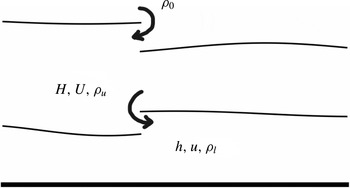
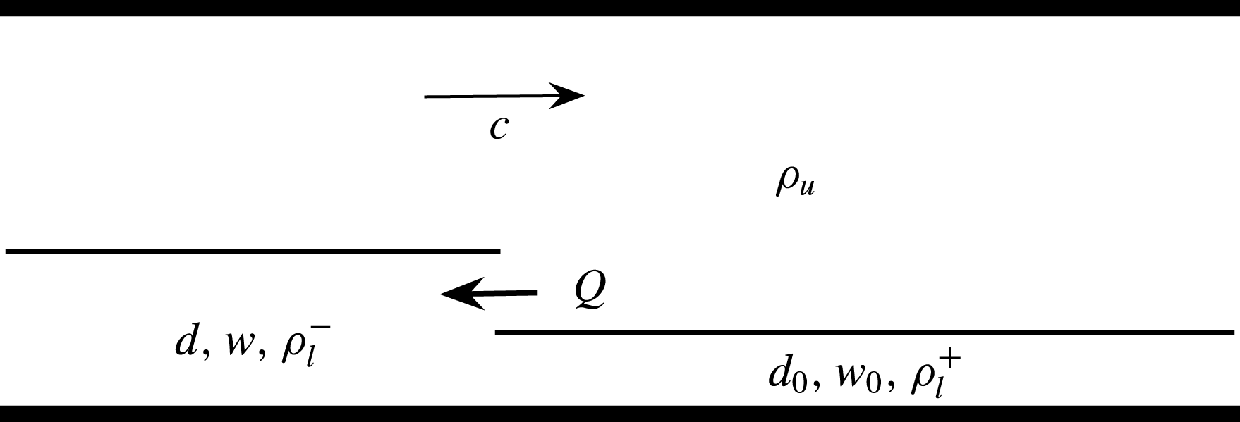
Sketch of the physical problem. Shown are the free surfaces and a baroclinic entraining shock. The horizontal bottom is at
 $z=0$
.

One of the simplest unsteady problems involving two-layer flows is the lock-exchange problem. This is the idealized situation where two fluids of different densities are initially confined to the left and right of a barrier, which is removed at
 $t=0$
. (The analogue with just one layer and a free surface is the dam-breaking problem.) We study the lock exchange as an application of the closure proposed in this article.
The paper is organized as follows. In § 2 we derive the governing equations for both the free-surface and the rigid-lid-bounded two-layer flows and their connection in the asymptotic limit of infinitely separated time scales. In § 3 we propose conservation-law-based mixing closures for both cases, and compute free-surface lock-exchange solutions. The consequences of using the energy closures in steady bores is also discussed. In § 4 we study the lock-exchange rigid-lid problem analytically under two extreme closures: volume conservation and energy conservation, corresponding to null and maximal mixing, respectively.
2. Formulation and governing equations
2.1. Two interfaces
Consider the configuration shown in figure 1, sometimes called the ‘two-and-a-half’-layer problem. We denote the height of the lower and upper active layers
 $h(x,t)$
and
 $H(x,t)$
, respectively, and their densities
 ${\it\rho}_{l}$
and
 ${\it\rho}_{u}$
. The semi-infinite ‘passive’ layer above has reference density
 ${\it\rho}_{0}$
. The pressure is assumed to be in hydrostatic balance, and also to be uniform in
 $x$
for large enough values of
 $z$
; it is therefore given by
 $$\begin{eqnarray}p=\left\{\begin{array}{@{}ll@{}}{\it\rho}_{l}g(h-z)+{\it\rho}_{u}gH+{\it\rho}_{0}g(H_{0}-H-h),\quad & 0<z<h,\\ {\it\rho}_{u}g(h+H-z)+{\it\rho}_{0}g(H_{0}-h-H),\quad & h<z<h+H.\end{array}\right.\end{eqnarray}$$
The vertically integrated pressures in each layer yield the hydrostatic forces
 $$\begin{eqnarray}\int _{layer}p\,\text{d}z=\left\{\begin{array}{@{}ll@{}}P_{s}^{l}={\textstyle \frac{1}{2}}({\it\rho}_{l}-{\it\rho}_{0})gh^{2}+({\it\rho}_{u}-{\it\rho}_{0})gHh+{\it\rho}_{0}g(H_{0}-{\textstyle \frac{1}{2}}h)h,\quad & \text{lower layer},\\ P_{s}^{u}={\textstyle \frac{1}{2}}({\it\rho}_{u}-{\it\rho}_{0})gH^{2}+{\it\rho}_{0}g(H_{0}(H-h)+h^{2}),\quad & \text{upper layer}.\end{array}\right.\end{eqnarray}$$
The form drag on each interface is
 $$\begin{eqnarray}F_{d}=\left\{\begin{array}{@{}ll@{}}F_{d}^{h}=({\it\rho}_{u}gH+{\it\rho}_{0}g(H_{0}-H-h))h_{x},\quad & \text{lower interface},\\ F_{d}^{h+H}={\it\rho}_{0}g(H_{0}-h-H)(h+H)_{x},\quad & \text{upper interface}.\end{array}\right.\end{eqnarray}$$
Thus, the resultant force in each layer
 $F=-P_{s}+F_{d}$
is
 $$\begin{eqnarray}F=\left\{\begin{array}{@{}ll@{}}-P_{s,x}^{l}+F_{d}^{h}=-({\it\rho}_{l}-{\it\rho}_{0})ghh_{x}-({\it\rho}_{u}-{\it\rho}_{0})ghH_{x},\quad & \text{lower layer},\\ -P_{s,x}^{u}+F_{d}^{h+H}-F_{d}^{h}=-({\it\rho}_{u}-{\it\rho}_{0})gHH_{x}-({\it\rho}_{u}-{\it\rho}_{0})gHh_{x},\quad & \text{upper layer}.\end{array}\right.\end{eqnarray}$$
We can write the conservation of volume and momentum in each layer, introducing the corresponding velocities
 $u(x,t)$
and
 $U(x,t)$
. For simplicity, we make the Boussinesq approximation, which is a scaling limit of the dynamics valid for small density differences between layers and used in many geophysical applications. The approximation entails using the densities of each layer in the ‘buoyancy’ terms derived above, but replacing them by a reference density (such as
 ${\it\rho}_{0}$
) in the inertial terms. We consider an approximation where the density changes resulting from entrainment and mixing do not affect the conservation laws. The more general case for ‘one-and-a-half’-layer models is discussed in Jacobsen et al. (Reference Jacobsen, Milewski and Tabak2008).
Thus, defining
 $$\begin{eqnarray}b\equiv g\frac{{\it\rho}_{l}-{\it\rho}_{0}}{{\it\rho}_{0}},\quad B\equiv g\frac{{\it\rho}_{u}-{\it\rho}_{0}}{{\it\rho}_{0}},\end{eqnarray}$$
the conservation laws for volume and the momentum equations read
 $$\begin{eqnarray}\displaystyle & h_{t}+(hu)_{x}=0, & \displaystyle\end{eqnarray}$$
 $$\begin{eqnarray}\displaystyle & (hu)_{t}+(hu^{2})_{x}+b({\textstyle \frac{1}{2}}h^{2})_{x}+BhH_{x}=0, & \displaystyle\end{eqnarray}$$
 $$\begin{eqnarray}\displaystyle & H_{t}+(HU)_{x}=0, & \displaystyle\end{eqnarray}$$
 $$\begin{eqnarray}\displaystyle & (HU)_{t}+(HU^{2})_{x}+B({\textstyle \frac{1}{2}}H^{2})_{x}+BHh_{x}=0. & \displaystyle\end{eqnarray}$$
 $$\begin{eqnarray}\displaystyle & \displaystyle u_{t}+({\textstyle \frac{1}{2}}u^{2}+bh+BH)_{x}=0, & \displaystyle\end{eqnarray}$$
 $$\begin{eqnarray}\displaystyle & \displaystyle U_{t}+({\textstyle \frac{1}{2}}U^{2}+B(h+H))_{x}=0. & \displaystyle\end{eqnarray}$$
The system (2.6)–(2.9) has six physically motivated scalar conservation laws of the form
 $$\begin{eqnarray}v_{t}+[Q(\boldsymbol{v})]_{x}=0,\end{eqnarray}$$
where the conserved quantities forming the vector
 $\boldsymbol{v}$
are functions of the physical variables, and the
 $Q$
are their fluxes: the two volume conservation equations (2.6) and (2.8), the two conservation laws for circulation
 $U$
and
 $w=u-U$
around each interface, resulting in (2.11) and the difference of (2.10) and (2.11),
 $$\begin{eqnarray}w_{t}+({\textstyle \frac{1}{2}}u^{2}-{\textstyle \frac{1}{2}}U^{2}+(b-B)h)_{x}=0,\end{eqnarray}$$
and laws for conservation of total momentum and total energy. These are, respectively, the sum of (2.7) and (2.9),
 $$\begin{eqnarray}P_{t}+(hu^{2}+HU^{2}+{\textstyle \frac{1}{2}}bh^{2}+BhH+{\textstyle \frac{1}{2}}BH^{2})_{x}=0,\end{eqnarray}$$
where
 $P=hu+HU$
, and
 $$\begin{eqnarray}E_{t}+[hu^{3}+HU^{3}+2(b-B)h^{2}u+2B(hu+HU)(h+H)]_{x}=0,\end{eqnarray}$$
where
 $E=hu^{2}+HU^{2}+(b-B)h^{2}+B(h+H)^{2}$
. It was proved in Barros (Reference Barros2006) that these are the only linearly independent conserved quantities. Whilst any set of four independent combinations of the above six laws yields identical dynamics for smooth solutions, once shocks form, the solutions differ considerably. In the remainder of the paper, we discuss various combinations of the above conservation laws that may be used to model problems in which the two fluids mix.
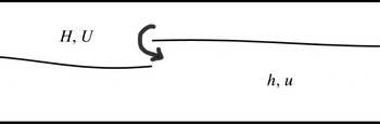
Schematic of the two-layer one-interface flow. A shock is shown entraining lighter fluid into heavier fluid, a situation considered later in the paper.

The characteristic speeds
 ${\it\lambda}$
of the system (2.6)–(2.9) satisfy
 $$\begin{eqnarray}[({\it\lambda}-u)^{2}-bh][({\it\lambda}-U)^{2}-BH]-B^{2}Hh=0,\end{eqnarray}$$
corresponding to two baroclinic and two barotropic modes. We will use this expression later when we show that the rigid-lid system results from an asymptotic decoupling of these modes. Notice that the speeds are real when the heights
 $h$
and
 $H$
are positive and
 $b>B$
and the shear between the layers
 $|u-U|$
is sufficiently small. At larger values of the shear, the system is ill-posed in time, a reflection of the Kelvin–Helmholtz instability criterion being achieved in the long-wave limit. In Chumakova et al. (Reference Chumakova, Menzaque, Milewski, Rosales, Tabak and Turner2009) it was shown that this type of instability threshold may be naturally reached during the smooth evolution of similar systems of
 $4\times 4$
equations, whereas this is not the case under the rigid-lid approximation.
2.2. One interface and rigid lid
The simplest set of evolution equations for interfacial waves arises in the situation in which the flow is bounded by two horizontal rigid lids as shown in figure 2. The formulation then differs somewhat, since a reference pressure is unknown a priori: the pressure at the top rigid lid follows not from the weight of fluid above it, but instead from enforcing incompressibility below. In the Boussinesq limit, the non-dimensional equations in smooth parts of the flow reduce to (see Long Reference Long1956; Milewski et al. Reference Milewski, Tabak, Turner, Rosales and Menzaque2004)
 $$\begin{eqnarray}\displaystyle & h_{t}+(uh)_{x}=0, & \displaystyle\end{eqnarray}$$
 $$\begin{eqnarray}\displaystyle & \displaystyle u_{t}+\frac{1-3h}{1-h}uu_{x}+\left((1-h)-\frac{1}{(1-h)^{2}}u^{2}\right)u_{x}=0. & \displaystyle\end{eqnarray}$$
 $$\begin{eqnarray}h+H=1,\quad uh+UH=0.\end{eqnarray}$$
The second constraint above corresponds to conservation of total momentum in the Boussinesq approximation and is used throughout this paper. For non-mixing layers (i.e. when each layer’s volume is conserved), this conservation of momentum is a consequence of volume conservation, the rigid-lid assumption and either the Boussinesq approximation or appropriate boundary conditions Boonkasame & Milewski (Reference Boonkasame and Milewski2011). The equations above have been non-dimensionalized as follows: layer depths with the total depth
 $D_{0}$
, velocities with
 $C=\sqrt{g(({\it\rho}_{l}-{\it\rho}_{u})/{\it\rho}_{l})D_{0}}$
and lengths and time with
 $D_{0}$
and
 $D_{0}/C$
, respectively.
These equations are similar to their one-layer shallow water counterparts, but with an apparently more complex nonlinearity. However, it was shown in Chumakova et al. (Reference Chumakova, Menzaque, Milewski, Rosales, Tabak and Turner2009) that, using the system’s Riemann invariants, one can build a nonlinear map between the smooth solutions of the two-layer flow system and those of one-layer shallow waters, providing a surprising connection between one- and two-layer flows. This connection was further explored in Esler & Pearce (Reference Esler and Pearce2011) in the study of non-mixing internal dam-break and lock-exchange flows, where it was found that, owing to the nature of the map, not all two-layer solutions can be uniquely mapped to one-layer flows. Whilst the system has similarities with one-layer shallow water, there are many differences: for example, the momentum in individual layers is not conserved, and, at shocks, the possibility of mixing must be considered.
Introducing the interfacial displacement and shear variables
 $$\begin{eqnarray}d\equiv h-H=2h-1,\quad w\equiv u-U=\frac{u}{1-h},\end{eqnarray}$$
one can symmetrize the system with volume and circulation conservation laws (Chumakova et al. Reference Chumakova, Menzaque, Milewski, Rosales, Tabak and Turner2009):
 $$\begin{eqnarray}\displaystyle & d_{t}+({\textstyle \frac{1}{2}}w(1-d^{2}))_{x}=0, & \displaystyle\end{eqnarray}$$
 $$\begin{eqnarray}\displaystyle & w_{t}+({\textstyle \frac{1}{2}}d(1-w^{2}))_{x}=0. & \displaystyle\end{eqnarray}$$
 $$\begin{eqnarray}{\it\lambda}^{\pm }=\text{d}w\pm {\textstyle \frac{1}{2}}\sqrt{(1-d^{2})\,(1-w^{2})},\end{eqnarray}$$
and can be written in the characteristic form as
 $$\begin{eqnarray}R_{t}^{\pm }+{\it\lambda}^{\pm }R_{x}^{\pm }=0,\end{eqnarray}$$
where
 $$\begin{eqnarray}R^{\pm }=\sin ^{-1}(d)\mp \sin ^{-1}(w)\end{eqnarray}$$
are the system’s Riemann invariants. The solutions were proved in Milewski et al. (Reference Milewski, Tabak, Turner, Rosales and Menzaque2004) to remain in the hyperbolic region
 $|d|<1,~|w|<1$
for all time. This is a sharp ‘nonlinear stability’ criterion for the equations, as it guarantees solutions to exist up to breaking, providing the initial shear is everywhere within the stability threshold
 $|w|<1$
(
 $w$
plays the role of a local Richardson number in this problem).
2.3. Decoupling of the baroclinic modes
Whilst the rigid-lid equations can be derived by assuming a priori the rigid-lid configuration in figure 2, they can also be found in the limit of the two-interface equations through the decoupling of the barotropic and baroclinic modes when their time scales are well separated. The separation of time scales occurs when the density difference at the lower interface is much smaller than that at the upper one:
 $$\begin{eqnarray}b=B+g\frac{{\it\rho}_{l}-{\it\rho}_{u}}{{\it\rho}_{0}}\equiv B+{\it\epsilon}.\end{eqnarray}$$
Introducing the variables
 $$\begin{eqnarray}d=h-H,\quad w=u-U,\quad D=h+H,\quad P=hu+HU,\end{eqnarray}$$
the shallow water equations (2.6)–(2.9) become
 $$\begin{eqnarray}\displaystyle & D_{t}+P_{x}=0, & \displaystyle\end{eqnarray}$$
 $$\begin{eqnarray}\displaystyle & \displaystyle P_{t}+\left(\frac{P^{2}}{D}+\frac{w^{2}}{4D}(D^{2}-d^{2})+\frac{1}{2}BD^{2}+{\it\epsilon}\frac{1}{8}(D+d)^{2}\right)_{x}=0, & \displaystyle\end{eqnarray}$$
 $$\begin{eqnarray}\displaystyle & \displaystyle d_{t}+\left(\frac{P}{D}d+\frac{1}{2D}(D^{2}-d^{2})w\right)_{x}=0, & \displaystyle\end{eqnarray}$$
 $$\begin{eqnarray}\displaystyle & \displaystyle w_{t}+\left(\frac{P}{D}w+\frac{1}{2D}({\it\epsilon}D-w^{2})d+{\it\epsilon}\frac{1}{2}D\right)_{x}=0. & \displaystyle\end{eqnarray}$$
 $$\begin{eqnarray}{\it\lambda}^{4}-(BD_{0}-{\it\epsilon}h_{0}){\it\lambda}^{2}+{\it\epsilon}Bh_{0}H_{0}=0.\end{eqnarray}$$
Thus the speeds separate into two pairs:
 $$\begin{eqnarray}{\it\lambda}^{2}=BD_{0}+O({\it\epsilon})\quad \text{and}\quad {\it\lambda}^{2}={\it\epsilon}\frac{h_{0}H_{0}}{D_{0}}+O({\it\epsilon}^{2}).\end{eqnarray}$$
In order to consider the limiting case
 ${\it\epsilon}\rightarrow 0$
and retain only the slow baroclinic modes, we rescale the fully nonlinear equations with
 $$\begin{eqnarray}t=\frac{1}{\sqrt{{\it\epsilon}}}\,\tilde{t},\quad w=\sqrt{{\it\epsilon}}\,\tilde{w},\quad D=1+{\it\epsilon}\,\tilde{D},\quad P={\it\epsilon}^{3/2}\,\tilde{P}.\end{eqnarray}$$
Dropping the tildes, the leading-order terms in the equations now read
 $$\begin{eqnarray}\displaystyle & d_{t}+({\textstyle \frac{1}{2}}(1-d^{2})w)_{x}=0, & \displaystyle\end{eqnarray}$$
 $$\begin{eqnarray}\displaystyle & w_{t}+({\textstyle \frac{1}{2}}(1-w^{2})d)_{x}=0, & \displaystyle\end{eqnarray}$$
 $$\begin{eqnarray}\displaystyle & \displaystyle \left(\frac{w^{2}}{4}(1-d^{2})+BD+\frac{1}{8}(1+d)^{2}\right)_{x}=0, & \displaystyle\end{eqnarray}$$
 $$\begin{eqnarray}\displaystyle & D_{t}+P_{x}=0. & \displaystyle\end{eqnarray}$$
 $D$
, whilst the last equation (2.38) defines an induced barotropic mean flow
 $P$
. The instantaneous nature of the adjustment of the barotropic variables
 $D$
and
 $P$
to the baroclinic ones
 $d$
and
 $w$
is a consequence of the scale separation between the two: in terms of the baroclinic time scale, the barotropic wave speed is effectively infinite.
The inverse of the transformation, under the scalings assumed, yields
 $$\begin{eqnarray}h=\frac{d+D}{2}=\frac{d+1}{2}+O({\it\epsilon}),\quad H=\frac{D-d}{2}=\frac{1-d}{2}+O({\it\epsilon}),\end{eqnarray}$$
 $$\begin{eqnarray}u=\frac{P}{D}+\frac{D-d}{2D}w=\sqrt{{\it\epsilon}}\,\frac{1-d}{2}w+O({\it\epsilon}^{3/2}),\quad U=\frac{P}{D}-\frac{D+d}{2D}w=-\sqrt{{\it\epsilon}}\,\frac{1+d}{2}w+O({\it\epsilon}^{3/2}).\end{eqnarray}$$
Substituting these values in
 $E$
gives
 $$\begin{eqnarray}E=B+\frac{{\it\epsilon}}{4}(2-(1-w^{2})(1-d^{2})+2d)+2{\it\epsilon}BD+o({\it\epsilon}).\end{eqnarray}$$
In the entrainment and mixing problem, we shall use the order-
 ${\it\epsilon}$
correction to the energy
 $2-(1-w^{2})(1-d^{2})+2d$
in the rigid-lid approximation to mimic the two-interface flow. Note that
 $BD$
, the last term of order
 ${\it\epsilon}$
, is omitted from this energy because it enforces volume conservation in the two lower layers, which is the only choice consistent with a rigid-lid limit.
3. Entrainment and mixing
In order to address flows with mixing and entrainment at shocks, one has to replace the volume conservation law by other choices. In this section, this issue is discussed for both the two-interface problem and the rigid-lid one-interface problem.
The general approach here extends and complements ideas presented in Jacobsen et al. (Reference Jacobsen, Milewski and Tabak2008), where we considered the ‘one-and-a-half’-layer model (one shallow water layer with an infinite layer of passive lighter fluid above). Within that context, we presented two main results: (i) For sufficiently supercritical flows, the maximum amount of mixing allowed at a shock is given explicitly by assuming that the shock has maximum speed, subject to the constraints provided by the conservation laws and the Lax condition. This result provides a strict upper bound for mixing. (ii) For subcritical flows, maximal mixing is attained by assuming that conservation of energy replaces conservation of volume. This provides an elegant and simple way to evolve mixing flows, an approach that we follow here. However, the problem here is more subtle, since the choice of conserved quantities (from an infinite set) is not obvious.
3.1. Mixing in the two-interface configuration
In general, mixing may occur at both interfaces. The simplest situation would arise when both layers’ volume conservation equations are discarded in favour of the remaining four conservation equations: the two circulations, total momentum and total energy. This is problematic though, since the four variables
 $u,U,hu+HU$
and
 $E$
do not carry sufficient information to uniquely define the layer heights: if
 $u=U=0$
, the transformation
 $(u,h,U,H)\leftrightarrow (u,P,U,E)$
is not invertible since
 $P=0$
and
 $E=(b-B)h^{2}+B(h+H)^{2}$
, providing one equation for the two heights.
Thus, one must instead make a priori assumptions relating the entrainment at both interfaces by using a linear combination of the two volume conservations as one of the laws. As an example, throughout this paper, we consider the case in which entrainment occurs only at the lower interface, a physically reasonable scenario for baroclinic flows. This can be accomplished by the following system of conservation laws:
 $$\begin{eqnarray}\displaystyle & D_{t}+[hu+HU]_{x}=0, & \displaystyle\end{eqnarray}$$
 $$\begin{eqnarray}\displaystyle & w_{t}+[{\textstyle \frac{1}{2}}u^{2}-{\textstyle \frac{1}{2}}U^{2}+(b-B)h]_{x}=0, & \displaystyle\end{eqnarray}$$
 $$\begin{eqnarray}\displaystyle & P_{t}+[hu^{2}+HU^{2}+{\textstyle \frac{1}{2}}bh^{2}+BhH+{\textstyle \frac{1}{2}}BH^{2}]_{x}=0, & \displaystyle\end{eqnarray}$$
 $$\begin{eqnarray}\displaystyle & E_{t}+[hu^{3}+HU^{3}+2(b-B)h^{2}u+2B(hu+HU)(h+H)]_{x}=0, & \displaystyle\end{eqnarray}$$
 $$\begin{eqnarray}\mathscr{Q}=-c[h]_{-}^{+}+[hu]_{-}^{+},\end{eqnarray}$$
where
 $c$
is the shock’s speed and
 $[\cdot ]_{-}^{+}$
indicates the jump in the enclosed quantity from left to right. The total rate of change of volume in the lower layer is then given by
 $$\begin{eqnarray}\frac{\text{d}}{\text{d}t}\int h\,\text{d}x=\mathop{\sum }_{shocks}\mathscr{Q}.\end{eqnarray}$$
The change of density in the lower layer in response to this entrainment is given by
 $$\begin{eqnarray}{{\it\rho}_{1}}_{t}+u_{1}({\it\rho}_{1})_{x}=\mathop{\sum }_{shocks}\frac{{\it\rho}_{2}-{\it\rho}_{1}}{h_{1}}\mathscr{Q}^{+}(t)\,{\it\delta}(x-s(t)),\end{eqnarray}$$
where
 $s(t)$
is the position of the shock and
 $\mathscr{Q}^{+}$
is the positive part of
 $\mathscr{Q}$
. Notice, though, that this is a diagnostic, a posteriori, calculation of
 ${\it\rho}_{1}$
that does not affect the dynamics: in models of the kind developed here, the densities are assumed constant throughout each layer. This can be thought of as a first-order approximation, quantitatively valid in situations where the density variations brought about by entrainment are not very big. It is possible to build models that include the density variation in the dynamics (see, for instance, Jacobsen et al. (Reference Jacobsen, Milewski and Tabak2008) for one such model in a ‘one-and-a-half’-layer setting). These models are more complex, and, since each layer may have a horizontal density gradient, only valid on time scales shorter than the resulting overturning circulations within each layer.
A general finite volume methodology for the numerical solution of general systems of hyperbolic equations with arbitrary conserved quantities is discussed in Kurganov, Noelle & Guergana (Reference Kurganov, Noelle and Guergana2001). This methodology is particularly appropriate for general conservation laws because it does not require the solution of Riemann problems. In addition to being conservative, this method automatically generated entropic solutions, with shocks that satisfy the Lax conditions.
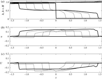
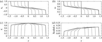
We show in figure 3 a typical solution arising from a form of the lock-exchange problem in the case of (3.1)–(3.4). The figure shows the surface displacements and velocities in each layer. This is a case where the density difference between the two layers is smaller than with the ambient by a factor
 ${\it\epsilon}=0.1$
. Thus, one sees a fast barotropic adjustment (see figure 3
b, where it is clear that at the first shown time a velocity disturbance is reaching the boundary) and the slow baroclinic flow, which consists of a buoyant gravity current propagating to the left and a heavy current propagating to the right. The upper interface deforms only slightly, rising on the side of the heavy current. Despite symmetric initial data, the asymmetry between the light and heavy currents is clear. This is mainly due to the asymmetry of entrainment: there is also a small contribution from the barotropic modes, but this source of asymmetry disappears as the difference in buoyancy between the two layers is made arbitrarily small.
Lock exchange in the two-interface flow with entrainment in the lower interface. The bold curves show the initial data and the final time. For this plot
 $b=1.1$
,
 $B=1.0$
and the initial data are
 $h=0.95$
for
 $x<0$
and
 $h=0.05$
for
 $x>0$
, with
 $h+H=1$
. At the lateral boundaries we have imposed conditions modelling a vertical wall. The solution is shown at times
 $t_{j}=j{\rm\Delta}t$
, with
 $j=0,\dots ,5$
and
 ${\rm\Delta}t=0.5/\sqrt{0.1}$
.

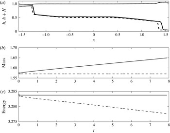
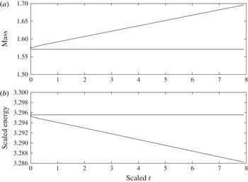
By comparing the results of figure 3 to the more classical model where conservation of volume is retained, the consequence of our model for entrainment is shown in figure 4. For this figure, we show the profiles from the entraining model and those resulting from solving the conservation laws for layer volumes and circulations: equations (2.6), (2.8), (2.10) and (2.11) with the same initial data. The results are shown in dashed lines. In figure 3(a), the interfacial positions at the final time are shown. Had the initial data been smooth, the evolution of the two solutions would have been identical up to breaking; with discontinuous initial data, however, they differ from
 $t=0$
. Clearly the solution of figure 3 has entrained fluid into the lower layer. Figure 3(b) shows that the total volume of the lower layer is an increasing function of time. Figure 3(c) shows the evolution of the total energy, which, in the volume conservation case, is dissipated at shocks.
Lock exchange in the two-interface flow. Comparison of entraining and non-entraining cases. The dashed line is the non-entraining case and the solid line is the entraining case of figure 3. (a) The final interfacial shapes; (b) the resulting total volume of the lower layer and (c) the total energy of the system.

The simulation just described is clearly dominated by the baroclinic modes, with the upper free surface barely deforming and slaved to the dynamics of the interface between the two active layers. Thus it is unnecessary to model it with two-and-a-half layers, whose computation is more expensive, principally because the fast modes pose time-stepping constraints. In addition, the rigid-lid assumption corresponds to the setting of many laboratory experiments. In § 4 we study the lock-exchange problem in the rigid-lid case, where the simplified equations allow us to write down the exact solution.
3.2. Conservation laws for the rigid-lid system
For 2 × 2 systems, there are in general infinitely many choices for conservation laws, where the conserved quantities themselves can be seen to obey a partial differential equation in the state space
 $d,w$
(see appendix A). From physical principles, one can verify that
 $$\begin{eqnarray}e\equiv -{\textstyle \frac{1}{4}}(1-d^{2})(1-w^{2})+{\textstyle \frac{1}{2}}{\it\alpha}(d+1)\end{eqnarray}$$
is the expression for the energy conserved by the system (2.21)–(2.22), where
 ${\it\alpha}$
is related to the reference height level at which potential energy is being measured. If one is intent on modelling mixing, the equation for volume conservation in each layer must be discarded. Instead, we replace it with energy conservation, where
 ${\it\alpha}$
can be used to control the relative strengths of entrainment into the layers.
This choice, for
 ${\it\alpha}\neq 0$
, breaks the symmetry imposed by the Boussinesq approximation. From the sign of
 $\partial e/\partial d$
at constant circulation, one can show that, for
 ${\it\alpha}\geqslant 1$
, the lower layer entrains fluid at shocks while the upper layer detrains it, and vice versa for
 ${\it\alpha}\leqslant -1$
. Note that, for
 $|{\it\alpha}|<1$
,
 $e$
does not depend monotonically on
 $d$
and therefore the system is ambiguous, as all dynamical variables cannot be recovered uniquely from the conserved quantities. In our entrainment simulations, we will make the choice
 ${\it\alpha}=1$
, corresponding to maximum entrainment into the lower layer. Note that conservation of mass instead of energy corresponds to the limit
 ${\it\alpha}\rightarrow \infty$
.
The fact that
 $\partial e/\partial d>0$
provides a simple proof that energy-preserving shocks maximize entrainment. Since energy cannot be created at the shock, the only alternative to energy conservation is energy dissipation. This would lead to a smaller volume in the lower layer due to the positive sign of
 $\partial e/\partial d$
. Hence energy-preserving shocks are maximally entraining among entropic solutions. Amongst energy-preserving shocks, the choice
 ${\it\alpha}=1$
is maximally entraining into the lower layer as
 $\partial e/\partial d$
is a minimum.
3.3. Steady bores
The simplest setting for the theory is that of an idealized bore, displayed in figure 5. A fluid with lower layer of height
 $h$
flows into a quiescent configuration with height
 $h_{0}\leqslant h$
(equivalently
 $d_{0}\leqslant d$
) and
 $u_{0}=w_{0}=0$
. The two unknowns are the speed
 $c$
of the shock and the velocity
 $u$
of the lower layer behind it (or the corresponding circulation
 $w$
). We shall now choose to conserve total energy and circulation (since total momentum is conserved automatically). This gives rise to the jump conditions
 $$\begin{eqnarray}\displaystyle & -c[e]_{-}^{+}+[q_{e}]_{-}^{+}=0, & \displaystyle\end{eqnarray}$$
 $$\begin{eqnarray}\displaystyle & -c[w]_{-}^{+}+[q_{w}]_{-}^{+}=0, & \displaystyle\end{eqnarray}$$
 ${\it\alpha}=1$
in (3.8) and thus
 $e=-((1-d^{2})(1-w^{2}))/4+(d+1)/2$
,
 $q_{e}=(wd(1-d^{2})(1-w^{2}))/4+w(1-d^{2})$
and
 $q_{w}=(d(1-w^{2}))/2$
, and the square brackets denote the jumps between the states ahead of and behind the shocks. Eliminating
 $c$
between the two jump conditions yields
 $$\begin{eqnarray}-\![q_{w}]_{-}^{+}[e]_{-}^{+}+[w]_{-}^{+}[q_{e}]_{-}^{+}=0,\end{eqnarray}$$
which after some algebra becomes
 $$\begin{eqnarray}\displaystyle & & \displaystyle \{d(1-d^{2})\}w^{4}+\{-(1+d)^{2}-(1-d^{2})(d_{0}+1)+d(d_{0}+1)^{2}\}w^{2}\nonumber\\ \displaystyle & & \displaystyle \qquad +\,\{(d_{0}-d)^{2}(d_{0}+d+2)\}=0,\end{eqnarray}$$
a bi-quadratic equation for
 $w$
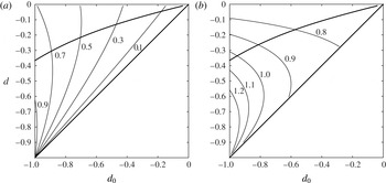
with only one real positive root. Figure 6 displays the Froude numbers
 $u/\sqrt{h}$
and
 $c/\sqrt{h}$
as functions of
 $d_{0}$
and
 $d$
. Also displayed is the curve marking the boundary of the domain of entropic shocks satisfying the Lax condition, whereby the characteristic speed
 ${\it\lambda}_{+}$
behind the shock is greater than or equal to the speed of the shock. Beyond this boundary, energy cannot be conserved without violating causality. This corresponds to the conceptual distinction between internal bores and hydraulic jumps proposed in Jacobsen et al. (Reference Jacobsen, Milewski and Tabak2008) in the context of a ‘one-and-a-half’-layer model: for maximal mixing, the active constraint for bores is energy conservation, while maximally mixing hydraulic jumps are constrained by the Lax entropy conditions. Here, we shall not consider entraining and energy-dissipating hydraulic jumps.
Schematic of steady shock travelling at speed
 $c$
into a quiescent fluid of density
 ${\it\rho}_{l}^{+}$
. The shock entrains fluid of density
 ${\it\rho}_{u}$
at rate
 $Q$
, which is assumed to mix behind the shock.

Properties of an energy-conserving shock of amplitude
 $d$
moving into a quiescent state of amplitude
 $d_{0}$
. (a) Contours of the downstream (oncoming flow) Froude number
 $u/\sqrt{h}$
. (b) Contours of the shock Froude number
 $c/\sqrt{h}$
. The upper bold curve corresponds to the limiting shock satisfying the Lax condition. Thus allowable shocks are inside the region bounded by the bold curves.

The uniform shock wave solution is well suited to study the consequences of entrainment. The calculations so far assumed that the lower layer has the same density ahead of and behind the shock. However, there is upper-layer fluid entrainment
 $\mathscr{Q}$
at the shock as given by (3.5), making the lower layer lighter behind the shock. Thus, the lower-layer density
 ${\it\rho}_{l}$
takes on two values,
 ${\it\rho}_{l}^{+}$
ahead of and
 ${\it\rho}_{l}^{-}$
behind the shock. To first order, one can use, for the jump conditions, an intermediate lower-layer density
 $\bar{{\it\rho}}$
, and then diagnose the actual densities before and after the shock in the presence of entrainment, introducing a density variation
 ${\rm\Delta}{\it\rho}$
such that
 $$\begin{eqnarray}{\it\rho}_{l}^{+}=\bar{{\it\rho}}+{\rm\Delta}{\it\rho},\quad {\it\rho}_{l}^{-}=\bar{{\it\rho}}-{\rm\Delta}{\it\rho}.\end{eqnarray}$$
From mass conservation in a control volume in the lower layer, the density change can be calculated, yielding
 $$\begin{eqnarray}\frac{{\rm\Delta}{\it\rho}}{\bar{{\it\rho}}-{\it\rho}_{u}}=~\frac{c(h-h_{0})-hu}{c(h+h_{0})-hu}.\end{eqnarray}$$
The entrainment
 $\mathscr{Q}$
and the relative density change
 ${\rm\Delta}{\it\rho}/(\bar{{\it\rho}}-{\it\rho}_{u})$
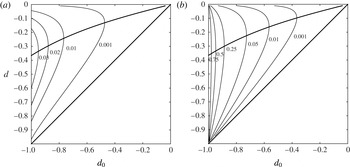
are displayed in figure 7. (Note that the relative density change is also equal to the relative change of the correspondingly defined buoyancies.) An extreme situation arises when
 $h_{0}=0$
, corresponding to a gravity current intruding into a fluid of uniform density
 ${\it\rho}_{0}$
. Here one obtains
 ${\rm\Delta}{\it\rho}=\bar{{\it\rho}}-{\it\rho}_{u}$
: behind the shock, the density is that of the upper layer. Clearly, for such dramatic density variation, the first-order approximation of computing the jump conditions as if there were no density change is not valid. The other limiting situation is the weak shock limit
 $h\approx h_{0}$
, with little entrainment. In this case the first-order approximation of uniform densities is valid.
Properties of an energy-conserving shock of amplitude
 $d$
moving into a quiescent state of amplitude
 $d_{0}$
. (a) Contours of the entrainment of upper fluid into the lower layer. (b) Contours of the density change across the shock in units of the mean density difference between the layers. The allowable shocks are inside the region bounded by the bold curves.

We note also that, in weakly non-hydrostatic long-wave models (such as Choi & Camassa Reference Choi and Camassa1999), there are smooth non-entraining energy-conserving solutions called ‘solibores’ (Esler & Pearce Reference Esler and Pearce2011), linking particular pairs of upstream and downstream depths.
4. Lock exchange for the rigid-lid system
In the previous section, we considered the consequences of entraining conservation laws on a steady bore. Here we turn our attention to an initial value problem. We consider the consequences of two different choices of conservation laws in the lock-exchange problem. In both cases we use conservation of circulation. This law relates the rate of change of circulation around the interface – the lower plume moving rightwards and the upper one moving leftwards – arising from the torque due to the pressure difference between the heavy and light fluid sides. The second conservation law is either layer volume (i.e. no entrainment) or energy, as used in the previous section (i.e. maximally efficient entrainment into the lower layer). It turns out that both scenarios can be solved in closed form, thus providing also a check on the numerical procedures used throughout this article.
The initial condition for a lock exchange has
 $w=0$
throughout and
 $$\begin{eqnarray}d=\left\{\begin{array}{@{}ll@{}}1,\quad & x<0,\\ -1,\quad & x>0.\end{array}\right.\end{eqnarray}$$
(In a more general case, the heavier fluid is only partially filling the left of the domain (see Ungarish Reference Ungarish2010), i.e.
 $d<1$
for
 $x<0$
; it can be treated similarly.)
4.1. Volume conservation
When (2.21)–(2.22) are adopted as the ruling conservation laws, the following jump conditions hold at shocks:
 $$\begin{eqnarray}\displaystyle & -c[d]_{-}^{+}+[{\textstyle \frac{1}{2}}w(1-d^{2})]_{-}^{+}=0, & \displaystyle\end{eqnarray}$$
 $$\begin{eqnarray}\displaystyle & -c[w]_{-}^{+}+[{\textstyle \frac{1}{2}}d(1-w^{2})]_{-}^{+}=0. & \displaystyle\end{eqnarray}$$
 $d=-1,~w=0$
ahead and
 $d_{+},~w_{+}$
behind, the equation for conservation of volume gives
 $$\begin{eqnarray}c={\textstyle \frac{1}{2}}w_{+}(1-d_{+}),\end{eqnarray}$$
which, inserted into the conservation of circulation, yields
 $$\begin{eqnarray}w_{+}^{2}=1+d_{+}.\end{eqnarray}$$
We can now close the problem for the front by computing the characteristic speeds for the system (2.21)–(2.22):
 $$\begin{eqnarray}{\it\lambda}=-wd\pm {\textstyle \frac{1}{2}}\sqrt{(1-d^{2})(1-w^{2})}.\end{eqnarray}$$
The speed
 $c$
of the shock, given by (4.29), must agree with the right-going characteristic speed immediately behind it. Thus,
 $$\begin{eqnarray}c={\textstyle \frac{1}{2}}w_{+}(1-d_{+})=-w_{+}d_{+}+{\textstyle \frac{1}{2}}\sqrt{(1-d_{+}^{2})(1-w_{+}^{2})}={\it\lambda}_{+}.\end{eqnarray}$$
This results in the full solution of the shock state with
 $$\begin{eqnarray}d_{+}=-{\textstyle \frac{1}{3}},\quad w_{+}=({\textstyle \frac{2}{3}})^{1/2}\approx 0.817,\quad c_{+}=({\textstyle \frac{2}{3}})^{3/2}\approx 0.544.\end{eqnarray}$$
This corresponds to a lower-layer depth of
 $h=1/3$
at the shock.
In order to proceed further and complete the solution for all
 $x$
ant
 $t$
, we use the fact that, because of the invariance under stretching of the equations and the initial conditions, the solution depends only on the similarity variable
 ${\it\xi}=x/t$
. Substituting this into the governing equations yields
 $$\begin{eqnarray}\displaystyle & -{\it\xi}d^{\prime }+({\textstyle \frac{1}{2}}w(1-d^{2}))^{\prime }=0, & \displaystyle\end{eqnarray}$$
 $$\begin{eqnarray}\displaystyle & -{\it\xi}w^{\prime }+({\textstyle \frac{1}{2}}d(1-w^{2}))^{\prime }=0. & \displaystyle\end{eqnarray}$$
 $w=w(d)$
, with
 $$\begin{eqnarray}\frac{\text{d}w}{\sqrt{1-w^{2}}}=\pm \frac{\text{d}d}{\sqrt{1-d^{2}}},\end{eqnarray}$$
resulting in
 $$\begin{eqnarray}\sin ^{-1}(w)=\pm \sin ^{-1}(d)+\sin ^{-1}(w_{0}),\end{eqnarray}$$
where
 $w_{0}=w|_{d=0}$
, and the sign corresponds to the Riemann invariant that is preserved across the rarefaction fan. Substituting the values we found previously behind the shock, we obtain that, when
 $d=0$
at the centre,
 $$\begin{eqnarray}w_{0}=\frac{5}{3\sqrt{3}}\approx 0.962,\quad {\it\lambda}=\pm {\it\lambda}_{0}=\pm \frac{1}{6}\sqrt{\frac{2}{3}}\approx \pm 0.136.\end{eqnarray}$$
Note that
 ${\it\lambda}_{0}=c_{+}/4$
. The full solution for
 $x>0$
consists of the shock at
 $x=c_{+}t$
, an expansion fan for
 $x\in ({\it\lambda}_{0}t,c_{+}t)$
, and a constant state
 $d=0,~w=w_{0}$
for
 $x\in [0,{\it\lambda}_{0}t]$
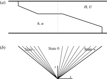
(refer to figure 8 for a schematic). The solution can be completed for
 $x<0$
by an odd extension of
 $d$
and an even extension of
 $w$
. Similar calculations of this type were shown in Rotunno et al. (Reference Rotunno, Klemp, Bryan and Muraki2011) for the non-Boussinesq volume-conservation case and using the Benjamin (Reference Benjamin1968) gravity current closure.
Two-layer lock-exchange schematic. (a) Physical configuration showing right- and left-going shocks trailed by expansions. The dotted line indicates the initial configuration. (b) Corresponding characteristic lines in the
 $x{-}t$
plane. The
 $\pm$
states are immediately behind the shocks.

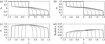
Figure 9 shows the lock-exchange solution to (2.21)–(2.22) computed numerically together with the exact solution derived above. In order to plot the lower-layer velocity, we rescaled
 $u$
with
 $\sqrt{{\it\epsilon}}$
, where
 ${\it\epsilon}=0.1$
to match the calculations of the full ‘two-and-a-half’-layer free-surface flow shown previously. Notice the very good agreement between the numerical and exact solutions shown at the last time in figure 9(b), as well as the good agreement with the numerical results in figure 3, which include a small barotropic fast mode.
4.2. Energy conservation and entrainment
We now consider an entraining case by replacing (4.2) with conservation of energy, resulting in the system
 $$\begin{eqnarray}\displaystyle & w_{t}+({\textstyle \frac{1}{2}}d(1-w^{2}))_{x}=0, & \displaystyle\end{eqnarray}$$
 $$\begin{eqnarray}\displaystyle & (-(1-d^{2})(1-w^{2})+2d)_{t}+(wd(1-d^{2})(1-w^{2})+w(1-d^{2}))_{x}=0. & \displaystyle\end{eqnarray}$$
 $$\begin{eqnarray}-\!c[-(1-d^{2})(1-w^{2})+2(d+1)]_{-}^{+}+[wd(1-d^{2})(1-w^{2})+w(1-d^{2})]_{-}^{+}=0.\end{eqnarray}$$
Eliminating
 $c$
between this equation and (4.3) gives
 $$\begin{eqnarray}w_{+}^{2}=\frac{d_{+}+1}{1-d_{+}},\quad c=\frac{1}{2}w_{+}(1-2d_{+}).\end{eqnarray}$$
Lock exchange in the one-interface rigid-lid flow with volume and circulation conservation. The bold curves show the initial data and the final time. The initial data are
 $d=1$
for
 $x<0$
and
 $d=-1$
for
 $x>0$
, and
 $w=0$
. At the lateral boundaries, we have imposed conditions modelling a vertical wall. The solution is shown at times
 $t_{j}=j{\rm\Delta}t$
, with
 $j=0,\dots ,5$
and
 ${\rm\Delta}t=0.5$
.

Substituting these relations into the expression for the characteristic speeds, we obtain a smaller-amplitude entraining hydraulic jump travelling faster than in the volume conservation case:
 $$\begin{eqnarray}d_{+}=\frac{1-\sqrt{3}}{2}\approx -0.366,\quad w_{+}=\sqrt{\frac{3-\sqrt{3}}{1+\sqrt{3}}}\approx 0.681,\quad c_{+}=\frac{\sqrt{3}}{2}\sqrt{\frac{3-\sqrt{3}}{1+\sqrt{3}}}\approx 0.590.\end{eqnarray}$$
This corresponds to a lower-layer depth
 $h=(3-\sqrt{3})/4\approx 0.317$
and an entrainment rate into the lower layer of
 $$\begin{eqnarray}-\!c[h]_{-}^{+}+[hu]_{-}^{+}=-\frac{c}{2}[d]_{-}^{+}+\left[\frac{1}{4}w(1-d^{2})\right]_{-}^{+}=\frac{1}{8}\sqrt{\frac{3-\sqrt{3}}{1+\sqrt{3}}}\;(2\sqrt{3}-3)\approx 0.0395.\end{eqnarray}$$
Unlike the non-entraining case, there is no right–left symmetry, and, in order to complete the solution, we need to solve also for the left-moving shock, with values ahead
 $d=1$
and
 $w=0$
. We obtain the equations
 $$\begin{eqnarray}\displaystyle & d_{-}(1+d_{-})w_{-}^{4}-(3+d_{-})w_{-}^{2}+(3+d_{-})(1-d_{-})=0, & \displaystyle\end{eqnarray}$$
 $$\begin{eqnarray}\displaystyle & \displaystyle c=\frac{1}{2w_{-}}(d_{-}(1-w_{-}^{2})-1), & \displaystyle\end{eqnarray}$$
 $d_{-}$
and
 $w_{-}$
are the values behind the left-going shock. Solving for the full shock conditions using the characteristic speeds must be done numerically and results in
 $$\begin{eqnarray}d_{-}\approx 0.337,\quad w_{-}\approx 0.858,\quad c_{-}\approx -0.531,\end{eqnarray}$$
with an upper-layer height
 $H\approx 0.332$
. This buoyant flow is mildly detraining, with
 $$\begin{eqnarray}-\!c[H]_{-}^{+}-[HU]_{-}^{+}=\frac{c}{2}[d]_{-}^{+}-\left[\frac{1}{4}w(1-d^{2})\right]_{-}^{+}\approx -0.014.\end{eqnarray}$$
Next, we compute the interior structure between the two shocks: behind each shock there is a rarefaction, and between the two rarefactions there is a constant state in the middle (see figure 8). Since these structures are continuous, the Riemann invariants are preserved along their corresponding characteristics, and thus the state in the middle has one Riemann invariant in common with each of the two states behind the shocks. Combining the
 $+$
Riemann invariant from behind the left-moving shock with the
 $-$
Riemann invariant from behind the right-moving shock, we find the state
 $(d_{0},w_{0})$
in between the two rarefaction fans:
 $$\begin{eqnarray}\displaystyle & R_{+}(d_{0},w_{0})=R_{+}(d_{-},w_{-})=\sin ^{-1}(d_{-})+\sin ^{-1}(w_{-}), & \displaystyle\end{eqnarray}$$
 $$\begin{eqnarray}\displaystyle & R_{-}(d_{0},w_{0})=R_{-}(d_{+},w_{+})=\sin ^{-1}(d_{+})-\sin ^{-1}(w_{+}). & \displaystyle\end{eqnarray}$$
 $$\begin{eqnarray}d_{0}=\sin \left(\frac{R_{+}+R_{-}}{2}\right)\approx 0.1253,\quad h_{0}\approx 0.5626,\quad w_{0}=\sin \left(\frac{R_{+}-R_{-}}{2}\right)\approx 0.9488.\end{eqnarray}$$
The back edges of the two expansion fans are given by
 $$\begin{eqnarray}{\it\lambda}={\it\lambda}=-d_{0}w_{0}\pm {\textstyle \frac{1}{2}}\sqrt{(1-d_{0}^{2})\,(1-w_{0}^{2})}\approx \left\{\begin{array}{@{}l@{}}0.0378,\quad \\ -0.2756.\quad \end{array}\right.\end{eqnarray}$$
Figure 10 shows the result of both the numerical solution of the entraining system and (in panel b) the comparison with the exact solution derived above. The profile of the interface can also be compared with the entrainment profile of the full ‘two-and-a-half’-layer system shown in figure 4. In figure 11 the total energy and layer volume of the entraining and non-entraining cases are shown as a function of time. The linear growth of the lower-layer volume in the energy-conserving case and the linear decrease in energy in the volume-conserving case are a consequence of the self-similar nature of the solution.
Lock exchange in the one-interface rigid-lid flow with entrainment. Circulation and energy conservation were chosen in order to attempt to mimic the two-interface model. The bold curves show the initial data and the final time. The initial data are
 $d=1$
for
 $x<0$
and
 $d=-1$
for
 $x>0$
, and
 $w=0$
. At the lateral boundaries we have imposed conditions modelling a vertical wall. The solution is shown at times
 $t_{j}=j{\rm\Delta}t$
, with
 $j=0,\dots ,5$
and
 ${\rm\Delta}t=0.5$
.


Our solution to the lock-exchange problem gives rise to non-uniform gravity currents entering a fluid of uniform density. In our model these have maximal entrainment but no mixing: the head of the wave is composed exclusively of entrained upper-layer fluid. In the self-similar scenario of the lock exchange, one can compute the width of this head: it grows linearly in time at a rate equal to the difference between the shock speed
 $c=0.59$
and the fluid velocity behind the shock,
 $u=((1-d)w)/2=0.47$
. Even though this scenario (corresponding locally to
 $d_{0}=-1$
in figures 6 and 7) is beyond the range of validity of the first-order closure that we use, and which calculates speeds by keeping the density in the lower layer unaltered, it provides speeds and solutions in good agreement with experimental observations. For example, simulations (Rotunno et al.
Reference Rotunno, Klemp, Bryan and Muraki2011) and experiments (Shin, Dalziel & Linden Reference Shin, Dalziel and Linden2004; Lowe, Rottman & Linden Reference Lowe, Rottman and Linden2005) show that, in the Boussinesq limit, the dimensionless right-going current speed is
 $c\approx 0.5$
. One further interesting consequence is the broken symmetry between left and right currents. The right-moving current has a speed about 10 % larger than the left-going one (which does not entrain). Such differences are observable in non-Boussinesq computations of the full Navier–Stokes equations and in experiments (see references above and figure 2(a) in Shin et al.
Reference Shin, Dalziel and Linden2004).
4.3. Comparison to non-mixing theory of Benjamin
There are several proposed closures in the literature for the speed of a gravity current (Benjamin Reference Benjamin1968; Huppert & Simpson Reference Huppert and Simpson1980; Shin et al.
Reference Shin, Dalziel and Linden2004). These have been applied to the lock-exchange problems (Ungarish Reference Ungarish2010; Rotunno et al.
Reference Rotunno, Klemp, Bryan and Muraki2011) by modelling the flow as two gravity currents. Here, we compare and contrast Benjamin’s original theory to ours. One may summarize Benjamin’s closure for the speed of a steadily travelling front as a function of the front height
 $h$
, through the formula
 $$\begin{eqnarray}\frac{c}{\sqrt{h}}=F_{B}(h)=\sqrt{\frac{(1-h)(2-h)}{(1+h)}}.\end{eqnarray}$$
This formula is obtained, under the Boussinesq approximation, by assuming: (i) a steady profile; (ii) conservation of volume; and (iii) conservation of momentum under the hydrostatic approximation.
Instead, our closure for general unsteady hydrostatic flows yields, by combining conservation of volume and circulation (i.e. (4.4) and (4.5)),
 $$\begin{eqnarray}F_{V}(h)=\sqrt{2}(1-h).\end{eqnarray}$$
By contrast, for the entrainment model with
 ${\it\alpha}=1$
, the combination of conservation of energy and circulation yields
 $$\begin{eqnarray}F_{E}(h)=\frac{1}{2}\frac{(3-4h)}{\sqrt{1-h}}.\end{eqnarray}$$
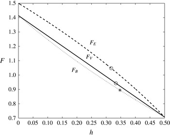
Both of these closures also have the assumption of conservation of momentum built in, as this is an intrinsic feature of the Boussinesq approximation (Boonkasame & Milewski Reference Boonkasame and Milewski2011; Camassa et al. Reference Camassa, Chen, Falqui, Ortenzi and Pedroni2012), where total mass flux and total momentum are equivalent. The comparison of these three closures is shown in figure 12.
Front speeds in gravity flows. The dotted line is Benjamin’s model, the solid line is the non-entraining case and the dashed line is the entraining case. The front height obtained using the characteristic speed condition (causality) is shown with circles.

Either of the three closures must be complemented by additional information to determine the speed and height of the front. In our case we use causality: the fact that the front cannot move faster than the speed of characteristics behind it. In the case of Benjamin’s closure, it has been complemented in various ways, for example, using conservation of energy in the original paper (Benjamin Reference Benjamin1968), leading to
 $h=1/2$
, or also using causality in Rotunno et al. (Reference Rotunno, Klemp, Bryan and Muraki2011), yielding
 $h=0.3473$
. The circles in figure 12 mark the location of the front speeds and heights in our solutions above, and the star marks the corresponding values in Rotunno et al. (Reference Rotunno, Klemp, Bryan and Muraki2011).
5. Conclusions
This article studies conservations laws for two-layer flows in hydrostatic balance and their implications for modelling entrainment. The simplest model for two-layer baroclinic flows has upper and lower rigid lids. The resulting system can be reduced to two equations in two unknowns with appealing symmetries. A tradeoff of this reduction is that the system admits infinitely many conservation laws, making the choice of two for a closed model somewhat arbitrary. By contrast, the more complete system with two layers and a free surface above has four degrees of freedom – two baroclinic and two barotropic modes – and only six independent conservation laws. Taking the limit of infinitely separated time scales between the barotropic and baroclinic modes in the free-surface model leads to a mapping to the conservation laws of physical relevance under the rigid-lid modelling assumption, which only captures the latter modes.
The systems are studied analytically and numerically for steady bores and for the unsteady lock-exchange problem, which has, as initial condition, fluids with different densities at rest to the left and right of a vertical wall that is instantly removed at time zero. In addition to this problem’s practical relevance, its extra symmetry under spatial and temporal stretching allows us to solve it exactly under the rigid-lid approximation, providing a benchmark for the theory as well as for the numerical methodology.
The article introduced a framework to study fluid entrainment in hydrostatic layered models. In order to do this in a conservation law setting, we replace the equation for volume conservation in each individual layer with conservation of energy. This conservation form, in fact, allows for the full range of dynamics: from mass conservation in each layer to maximum entrainment. The lock-exchange problem is solved in both limits. Intermediate cases could be chosen to model a mixing efficiency in flows that both mix and dissipate energy. In the particular setting of the lock-exchange problem, we compare our results with other (non-entraining) models in the literature.
Acknowledgements
The work of E.G.T. and P.A.M. was partially supported by the Division of Mathematical Sciences of the National Science Foundation, under grant number DMS-1211298. P.A.M. also acknowledges the generous support from a Royal Society Wolfson award.
Appendix A. Conservation laws in 2 × 2 systems
A general 2 × 2 system of equations of the form
 $$\begin{eqnarray}\displaystyle & & \displaystyle u_{t}+au_{x}+bv_{x}=0,\end{eqnarray}$$
 $$\begin{eqnarray}\displaystyle & & \displaystyle v_{t}+cu_{x}+dv_{x}=0\end{eqnarray}$$
 $q$
satisfying
 $[q(u,v)]_{t}+[Q(u,v)]_{x}=0$
if and only if
 $q$
satisfies the constraint in the form of a semilinear partial differential equation
 $$\begin{eqnarray}(aq_{u}+cq_{v})_{v}-(bq_{u}+dq_{v})_{u}=0.\end{eqnarray}$$
Applying this to the system (2.21)–(2.22) results in
 $$\begin{eqnarray}(w^{2}-1)q_{ww}-(d^{2}-1)q_{dd}=0.\end{eqnarray}$$
The conservations of volume and vorticity
 $q=d$
and
 $q=w$
are immediate, as is the conservation of
 $q=wd$
. One can easily check that the energy
 $e$
as defined previously also satisfies this equation. In fact, denoting
 $q=wd$
, the system (2.21)–(2.22) can be rewritten as
 $$\begin{eqnarray}\displaystyle & e_{t}+(qe)_{x}=0, & \displaystyle\end{eqnarray}$$
 $$\begin{eqnarray}\displaystyle & q_{t}+({\textstyle \frac{1}{2}}q^{2}+e)_{x}=0. & \displaystyle\end{eqnarray}$$
 $\mathit{eq}$
(‘momentum’) and
 $\mathit{eq}^{2}/2+e^{2}/2$
(‘energy’).