


1. Introduction
Turbulent thermal convection is ubiquitous in nature and in engineering applications. Rayleigh–Bénard convection (RBC), which concerns a confined fluid layer heated from below and cooled from above, is a paradigmatic system for studying turbulent thermal convection. The RBC system has received extensive interest in the past few decades (for reviews, see, for example, Ahlers, Grossmann & Lohse (Reference Ahlers, Grossmann and Lohse2009), Lohse & Xia (Reference Lohse and Xia2010), Chillà & Schumacher (Reference Chillà and Schumacher2012) and Xia (Reference Xia2013)). The control parameters of the RBC system are the Rayleigh number  $Ra = \alpha g H^3 \Delta T / \nu \kappa$ and the Prandtl number
 $Pr = \nu / \kappa$, wherein
 $\alpha$ is the thermal expansion coefficient,
 $g$ is the gravitational acceleration,
 $H$ is the cell height,
 $\Delta T$ is the temperature difference across the fluid layer, and
 $\nu$ and
 $\kappa$ are the kinematic viscosity and the thermal diffusivity of the working fluid, respectively.
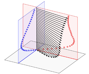
In fully developed RBC, viscous and thermal boundary layers (BLs) are developed near the isothermal surfaces. These BLs are crucial in determining the transport properties in RBC. The characterisation of the viscous BL properties is essential not only for providing insights into the physical nature, but also for the modelling of the turbulent thermal convection problem. Over the past few decades, BL properties have been extensively studied experimentally. For example, using a novel light scattering technique, Xin, Xia & Tong (Reference Xin, Xia and Tong1996) conducted the first systematic measurement of the viscous BL profile. The laser Doppler anemometry technique was also applied to measure the mean horizontal velocity (e.g. du Puits, Resagk & Thess Reference du Puits, Resagk and Thess2007; Li et al. Reference Li, Shi, Du Puits, Resagk, Schumacher and Thess2012). However, these single-point measurement techniques cannot obtain the instantaneous BL profiles. In recent years, the planar particle image velocimetry (PIV) technique has been applied to study the viscous BL properties of the RBC system in the mean large-scale circulation (LSC) plane (Xia, Sun & Zhou Reference Xia, Sun and Zhou2003; Sun, Xia & Tong Reference Sun, Xia and Tong2005; Sun, Cheung & Xia Reference Sun, Cheung and Xia2008; Zhou & Xia Reference Zhou and Xia2010; Zhou et al. Reference Zhou, Stevens, Sugiyama, Grossmann, Lohse and Xia2010; Wei & Xia Reference Wei and Xia2013). In a cylindrical convection cell, the LSC presents complicated flow dynamics including meandering (Cioni, Ciliberto & Sommeria Reference Cioni, Ciliberto and Sommeria1997; Funfschilling & Ahlers Reference Funfschilling and Ahlers2004; Ahlers, Brown & Nikolaenko Reference Ahlers, Brown and Nikolaenko2006; Xi, Zhou & Xia Reference Xi, Zhou and Xia2006; Xi & Xia Reference Xi and Xia2008; Zhu & Zhou Reference Zhu and Zhou2021), torsional (Funfschilling, Brown & Ahlers Reference Funfschilling, Brown and Ahlers2008) and sloshing (Xi et al. Reference Xi, Zhou, Zhou, Chan and Xia2009; Zhou et al. Reference Zhou, Xi, Zhou, Sun and Xia2009; Vogt et al. Reference Vogt, Horn, Grannan and Aurnou2018). For such a three-dimensional (3-D) configuration, given the potential effects of the complex motions of the LSC, the velocity components in the mean LSC plane alone may not be sufficient to fully characterise the instantaneous BL properties. The present work aims to address this problem by measuring the full velocity profile of the viscous BL using two synchronised cameras in orthogonal vertical planes. In order to eliminate the LSC effect, we propose to reconstruct the measured full velocity profile using a dynamic frame based on the changing directions of the instantaneous wall-shear stress.
The eddy viscosity, which quantifies the turbulent momentum transport, can be introduced into the BL equation describing the mean velocity profile (Schlichting & Gersten Reference Schlichting and Gersten2017). Using a vertical thin disk as a quasi-two-dimensional (quasi-2-D) configuration, Xu et al. (Reference Xu, Wang, He, Wang, Schumacher, Huang and Tong2021) conducted direct numerical simulations and found that the eddy viscosity profiles overlap for different Rayleigh numbers and exhibit a cubic power law with the wall distance. Note that almost all existing BL theories are based on 2-D BL equations, while the applicability of the theories for the 3-D convection cell is unclear. With the measured full viscous BL profile, the present work will help resolve this problem by studying the eddy viscosity properties in a cylindrical convection cell.
The energy dissipation rate, as perhaps the single most important quantity in the study of turbulence, plays a key role in the understanding and modelling of the RBC system, e.g. the renowned Grossmann–Lohse model (Grossmann & Lohse Reference Grossmann and Lohse2000, Reference Grossmann and Lohse2001) and the dissipation layer theory (Petschel et al. Reference Petschel, Stellmach, Wilczek, Lülff and Hansen2013). However, a high precision measurement of the energy dissipation rate profile requires all nine components of the velocity gradient tensor to be resolved and is beyond the reach of state-of-the-art experimental techniques. Ni, Huang & Xia (Reference Ni, Huang and Xia2011) indirectly measured the energy dissipation rate by 3-D particle tracking velocimetry in the central region of the cell. They found that the mean dissipation rate follows a power-law scaling  $Ra^{1.55 \pm 0.02}$, and revealed a local balance between the energy dissipation rate and the heat flux in the bulk region. Note that in their work, the second-order structure function in the dissipative range was used to estimate the mean dissipation rate, which requires that the flow satisfying local homogeneity and isotropy in the measurement region. In a subsequent study, Li et al. (Reference Li, Huang, Ni and Xia2021) obtained the energy dissipation rate in plume-abundant regions and found a power-law scaling
 $Ra^{1.34 \pm 0.07}$, suggesting that the flow dynamics in these plume-abundant regions are jointly determined by thermal plumes and turbulent background fluctuations. To the best of our knowledge, the energy dissipation rate at the solid boundary has not been measured experimentally in the RBC system. With the measured full velocity profile, the energy dissipation rate at the centre of the bottom plate can be directly obtained.
The remainder of this paper is organised as follows. We first present the experimental set-up, data acquisition and processing techniques in § 2. Our main results are then presented in § 3, which is further divided into three subsections. In § 3.1, we introduce the velocity reconstruction from the static laboratory frame to the dynamic wall-shear frame, and compare the properties of the viscous BL in both frames. In § 3.2, we present the unified power-law scaling relation of the turbulent eddy viscosity in the dynamic frame. In § 3.3, we show results of the energy dissipation rate at the centre of the bottom plate. Finally, we summarise our findings and conclude in § 4.
2. The experimental set-up
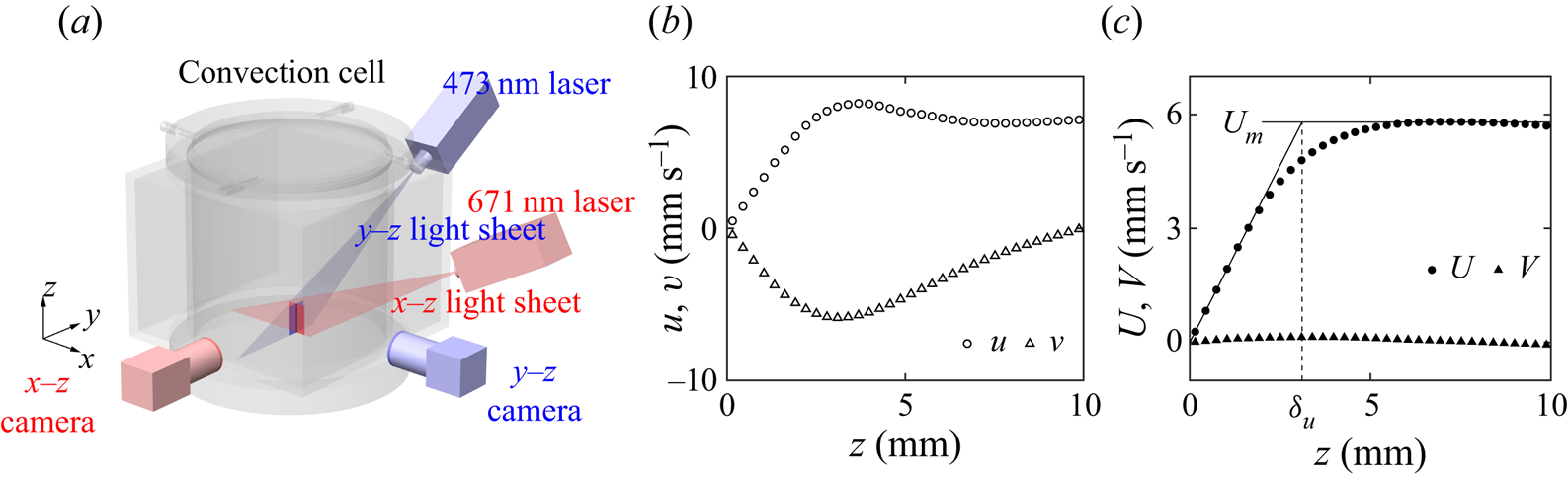
We used a cylindrical convection cell with its height and inner diameter both being 188 mm (aspect ratio  $\varGamma = 1$), as shown in figure 1(a). The top and bottom conducting plates are made of sapphire and copper, respectively, and the sidewall is made of 6 mm-thick Plexiglas. The upper surface of the bottom plate protrudes above the flange of the sidewall jacket to ensure no optical path blockage. To reduce image distortion caused by the curved sidewall, a water-filling square jacket was fitted around the cylinder. The convection cell was placed inside a thermostat whose temperature is set to the mean value of the convecting fluid (
 $T_c = 40\,^\circ {\rm C}$). Vibration sources, including the thermostat circulating fans and laser controllers, were carefully isolated from the optical table to minimise interference with the high-resolution experiment.
(a) Sketch of the cylindrical convection cell, the PIV measurement system and the Cartesian coordinates. Sample of (b) the instantaneous velocity  $u$,
 $v$ and (c) the time-averaged velocity
 $U$,
 $V$ along the intersectional line of two planar PIV images as a function of the wall distance
 $z$ at
 $Ra = 1.01 \times 10^9$. Panel (c) also illustrates the determination of the viscous BL thickness
 $\delta _u$ using the slope method from the near-wall velocity gradient
 $\partial U / \partial z$ and the maximum horizontal velocity
 $U_m$.

We applied a time-resolved PIV technique to measure the full velocity profile at the intersection of two planar velocity fields simultaneously. The convecting fluid was seeded with 10  $\mathrm {\mu }$m diameter hollow glass particles which were found to be 3–5 pixels in the camera image. Two continuous lasers with respective wavelengths of 473 and 671 nm formed two vertically orthogonal laser sheets each with 0.5 mm thickness. To minimise reflections, the upper surface of the bottom plate was coated with black nickel and the position of each laser was carefully adjusted to ensure a large incidence angle. Each camera lens was covered with a bandpass filter (
 $\pm$10 nm OD4) with its centre wavelength corresponding to the respective laser wavelength in the measurement plane. We used hollow glass spheres rather than polyamid seeding particles to reduce the laser reflection from the sedimented seeding particles on the bottom plate surface. The seeding particles were centrifuged to match the density of the working fluid prior to injection, thereby reducing their sedimentation during measurements. Two synchronised scientific CMOS cameras (pco.edge 5.5 with 5.5 megapixel, 16 bit dynamic range) with microlenses (Nikkor AF 105 mm
 $f/2.8$) were applied to record the PIV image sequences. In the measurement, the PIV image is
 $800 \times 2560$ pixels in size with 9.21
 $\mathrm {\mu }$m pixel
 $^{-1}$ resolution, corresponding to a
 $7.3\ {\rm mm}\times 23.5\ {\rm mm}$ (horizontal
 $\times$ vertical) field of view. We used Camera Link HS connection between the camera and the disc array to ensure an uncompressed long-term high frame-rate data transmission. In calibration, the convection cell was placed on a multiaxis heavy-load translation stage and the tip of a steel needle (
 $\approx$30
 $\mathrm {\mu }$m in diameter) was used as the calibration target. By moving the calibration target to a certain distance and recording its corresponding displacement on the image, the calibration parameters can be obtained. The calibration needle was removed prior to the PIV measurement. The Cartesian coordinate in the static laboratory frame, as shown in figure 1(a), is defined with its origin at the centre of the bottom plate,
 $x$–
 $y$ being the horizontal plane and the
 $z$ axis pointing upward. As with previous experiments (Sun & Xia Reference Sun and Xia2005; Xi et al. Reference Xi, Zhou, Zhou, Chan and Xia2009; Wei & Xia Reference Wei and Xia2013), the cylindrical convection cell was tilted by
 $1.55 \pm 0.05 ^{\circ }$ in the
 $x$–
 $z$ plane to partially lock the orientation of the LSC (so that the
 $y$-axis is now perpendicular to the mean plane of the LSC).
In the experiment, we used deionised and degassed water as the working fluid. The measurements covered the Rayleigh range  $1.82 \times 10^8$–
 $5.26 \times 10^9$ at a fixed Prandtl number
 $Pr = 4.34$. The PIV image sequence was acquired at a 80 Hz frame rate for 10.5 h at each Rayleigh number, corresponding to
 $3 \times 10^6$ snapshots in each measurement plane. The measurements covered
 $5\times 10^3$–
 $2.4 \times 10^4$ free-fall time units (
 $t_f \equiv \sqrt {H / (\alpha g \Delta T)}$) and thus ensured sufficient time-resolved statistics.
We applied an in-house cross-correlation code based on PIVlab (Thielicke & Sonntag Reference Thielicke and Sonntag2021) and high-performance computing facilities to process the large amount of PIV image data. Each frame was divided into interrogation areas of  $64 \times 64$ pixels with
 $50\,\%$ overlap, which corresponds to
 $23 \times 78$ velocity vectors. Therefore, the applied spatial resolution for the velocity profile intersecting at two vertical measurement planes is 0.29 mm. The velocity fields were validated using both global velocity range and local median check criteria to discard spurious values.
3. Results and discussions
3.1. Wall-shear stress and velocity reconstruction in the dynamic frame
The local wall-shear stress can be calculated using the vertical gradients of the horizontal velocity components at the centre of the bottom plate. Figure 1(b,c) shows samples of the instantaneous and mean profiles of the horizontal velocity components at  $Ra = 1.01 \times 10^9$, respectively. We see that the linear sections of the near-wall BL profiles can be accurately resolved by the present measurement. The velocity gradients
 $(\partial u / \partial z)|_{z = 0}$ and
 $(\partial v / \partial z)|_{z = 0}$ are obtained by a least-square fitting of the corresponding linear section close to the wall surface, and the wall-shear stress
 $\boldsymbol {\tau }$ is calculated as
 \begin{equation} \boldsymbol{\tau} = (\tau_x, \tau_y) = \left(\left. \mu \frac{\partial u}{\partial z} \right|_{z = 0}, \left. \mu \frac{\partial v}{\partial z} \right|_{z = 0} \right), \end{equation}
wherein  $\mu$ is the dynamic viscosity.
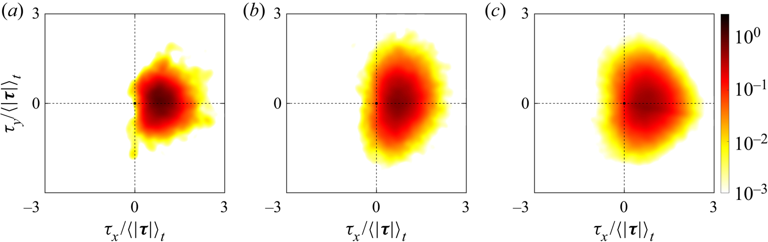
Figure 2 shows the joint probability density function (p.d.f.) of the two wall-shear stress components at three different Rayleigh numbers. We can see that there exist strong fluctuations in  $\tau _y$ which are comparable in magnitude with
 $\tau _x$, despite the fact that the convection cell has been tilted along the
 $x$ direction. As
 $Ra$ increases, the joint p.d.f. becomes more extended for both components. The probability of
 $\tau _{x}$ against the orientation of the mean LSC, i.e.
 $\tau _{x} < 0$, also becomes higher as
 $Ra$ increases. This may originate from the complicated 3-D motions of the LSC in the cylindrical cell including meandering, torsional and sloshing motions.
Joint p.d.f. of normalised wall-shear stress components at Rayleigh numbers (a)  $Ra = 1.82 \times 10^8$, (b)
 $Ra = 1.01 \times 10^9$ and (c)
 $Ra = 5.26 \times 10^9$.

Given the observed strong fluctuations of the local wall-shear stress, the single horizontal velocity component in the mean LSC plane may not be sufficient to characterise the instantaneous viscous BL. With the measured full velocity profile, we propose to reconstruct the near-wall velocity using a dynamic wall-shear frame based on the measured instantaneous wall-shear stress (hereafter we refer to this as the dynamic frame, with quantities obtained in this frame marked with superscript  $d$). The direction (projection angle) of the wall-shear stress
 $\phi$ is defined as
 \begin{equation} \phi \equiv {\rm{arctan}}{(\tau_y / \tau_x)}, \end{equation}
and the corresponding transformation matrix  $R$ as
 \begin{equation} R = \left[\begin{array}{ccc} {\cos \phi} & {\sin \phi} & 0 \\ {-\sin \phi} & {\cos \phi} & 0 \\ 0 & 0 & 1 \end{array}\right]. \end{equation}
The velocity vector in the dynamic frame  $(u^d, v^d, w^d)$ can thus be transformed from the laboratory frame
 $(u, v, w)$ following
 $R$. The vertical velocity remains unchanged after the transformation, i.e.
 $w^d = w$.
The viscous BL thicknesses in the respective frames  $\delta _u$ and
 $\delta _u^d$ are obtained using the slope method (see figure 1c), i.e. the distance at which the extrapolated linear section intersects the maximum velocity (Xin et al. Reference Xin, Xia and Tong1996),
 \begin{gather} \delta_u \equiv \frac{U_m}{({\partial U}/{\partial z})|_{z = 0}}, \end{gather}
 \begin{gather}\delta_u^d \equiv \frac{U_m^d}{({\partial U^d}/{\partial z})|_{z = 0}}, \end{gather}
wherein  $U \equiv \langle u \rangle _{t}$ and
 $U^d \equiv \langle u^d \rangle _{t}$ are the time-averaged velocities, the operator
 $\langle \,\cdot \, \rangle _t$ denotes the time-averaging, and
 $U_m \equiv \max (U)$ and
 $U_m^d \equiv \max (U^d)$ are the maximum velocities. The difference between
 $\delta _u$ and
 $\delta _u^d$ results from the inapplicability of the projection equation for the maximum horizontal velocity, i.e.
 $u_m \ne \cos (\phi ) u_m^d$ (
 $u_m \equiv \max (u)$,
 $u_m^d \equiv \max (u^d)$). The rotating transformation is strictly satisfied only in the linear section of the velocity profile, i.e.
 $u = \cos (\phi ) u^d$ in the linear section of the
 $u(z)$ profile. Above the linear section,
 $u(z)$ and
 $v(z)$ may present different shapes, resulting in
 $u \ne \cos (\phi ) u^d$ and thus
 $u_m \ne \cos (\phi ) u_m^d$. For example, for the instantaneous velocity profiles in figure 1(b),
 $\delta _u = 2.541$ mm while
 $\delta _u^d = 2.309$ mm.
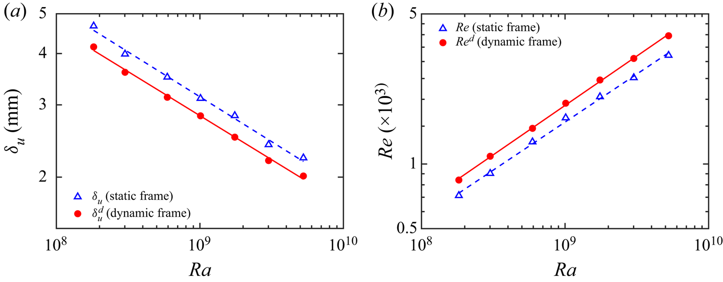
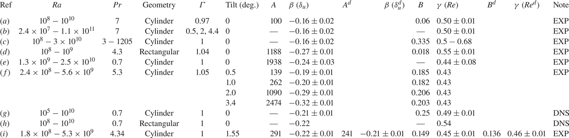
Figure 3(a) plots the viscous BL thickness as a function of the Rayleigh number, indicating a thinner viscous BL in the dynamic frame than in the laboratory frame. Whereas the power-law scaling exponents with  $Ra$ in two frames are essentially the same. As indicated in table 1, the scaling exponent of
 $\delta _u$ with
 $Ra$ has a larger value (i.e. a smaller magnitude) in Xin et al. (Reference Xin, Xia and Tong1996), Xin & Xia (Reference Xin and Xia1997) and Lam et al. (Reference Lam, Shang, Zhou and Xia2002), which is probably related to the dynamics of the LSC in the levelled cylindrical convection cell. Figure 3(b) plots the Reynolds number
 $Re = U_m H / \nu$ (
 $Re^d = U_m^d H / \nu$) as a function of
 $Ra$ in both frames, which characterises the intensity of the LSC. Fitting a power law to the data points yields
 $Re \sim Ra^{0.45}$ and
 $Re^d \sim Ra^{0.46}$ in the two frames, respectively. We also calculate the scaling of the viscous BL thickness with the Reynolds number by applying the data points in figure 3. The results of
 $\delta _u \sim Re^{-0.48}$ and
 $\delta _u^d \sim (Re^d)^{-0.47}$ basically satisfy the prediction of the classical Prandtl–Blasius BL, i.e.
 $\delta _u \sim Re^{-0.5}$. Our results are consistent with the fact that, for moderate Rayleigh number range, the viscous BL is still laminar albeit with fluctuations (Tilgner, Belmonte & Libchaber Reference Tilgner, Belmonte and Libchaber1993; Verzicco & Camussi Reference Verzicco and Camussi2003; Xia et al. Reference Xia, Sun and Zhou2003; Funfschilling & Ahlers Reference Funfschilling and Ahlers2004; Stevens et al. Reference Stevens, Zhou, Grossmann, Verzicco, Xia and Lohse2012; Scheel & Schumacher Reference Scheel and Schumacher2014). In the recent BL model of Ching et al. (Reference Ching, Leung, Zwirner and Shishkina2019) for turbulent RBC, the scaling of the viscous BL thickness is also proportional to
 $Re^{-0.5}$.
(a) The viscous BL thickness  $\delta _u$ and
 $\delta _u^d$ as a function of
 $Ra$. The fitted power-laws to the respective data are
 $\delta _u = 291 Ra^{-0.22 \pm 0.01}$ mm (blue dashed line) and
 $\delta _u^d = 241 Ra^{-0.21 \pm 0.01}$ mm (red solid line). (b) The Reynolds number
 $Re = U_m H / \nu$ and
 $Re^d = U_m^d H / \nu$ based on the maximum horizontal velocity as a function of
 $Ra$. The fitted power-laws of the respective data are
 $Re = 0.149 Ra^{0.45 \pm 0.01}$ (blue dashed line) and
 $Re^d = 0.136 Ra^{0.46 \pm 0.01}$ (red solid line).

Scaling exponents of the viscous BL thickness  $\delta _u$ (
 $\delta _u^d$) and the Reynolds number
 $Re$ (
 $Re^d$) as a function of the Rayleigh number
 $Ra$. The coefficients
 $A$ and
 $B$, and scaling exponents
 $\beta$ and
 $\gamma$ are determined from the power laws
 $\delta _u = A Ra^{\beta }$ (
 $\delta _u^d = A^d Ra^{\beta }$) and
 $Re = B Ra^{\gamma }$ (
 $Re^d = B^d Ra^{\gamma }$). The coefficients
 $A$ and
 $A^d$ are in units of millimetres. The control parameters
 $Ra$,
 $Pr$, the cell geometry and the aspect ratio
 $\varGamma$ are also listed. The sources are (a) Xin et al. (Reference Xin, Xia and Tong1996), (b) Xin & Xia (Reference Xin and Xia1997), (c) Lam et al. (Reference Lam, Shang, Zhou and Xia2002), (d) Sun et al. (Reference Sun, Cheung and Xia2008), (e) Li et al. (Reference Li, Shi, Du Puits, Resagk, Schumacher and Thess2012), (f) Wei & Xia (Reference Wei and Xia2013), (g) Scheel & Schumacher (Reference Scheel and Schumacher2014) (h) Zou et al. (Reference Zou, Zhou, Chen, Bao, Chen and She2019) and (i) present work. Abbreviations are: direct numerical simulation (DNS); experiment (EXP). The tilt angle of the convection cell is considered to be zero when not explicitly mentioned in the respective sources.

3.2. The eddy viscosity and the mean velocity profile
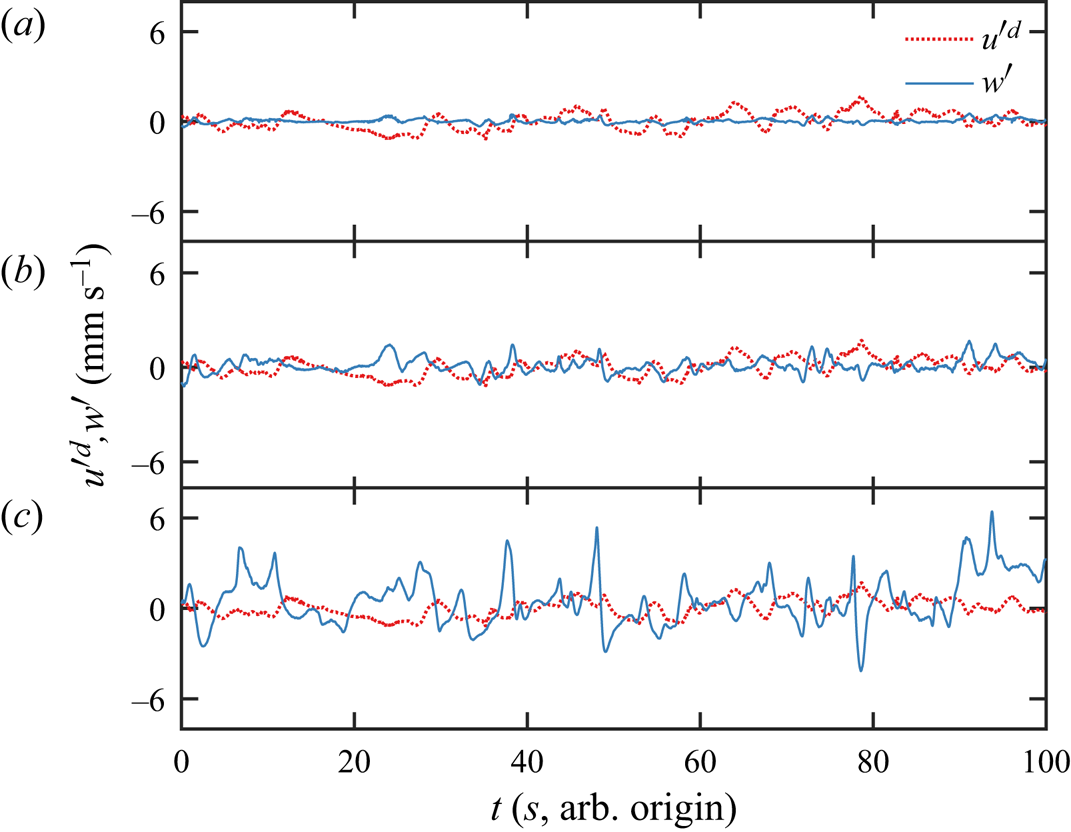
Figure 4 plots time traces of velocity fluctuation components  ${u'}^d$ and
 $w'$ in the dynamic frame at different wall distances. Deep inside the viscous BL at
 $z / \delta _u^d = 0.2$, the magnitudes of
 ${u'}^d$ and
 $w'$ are small, and a close inspection of the two time traces reveals a negative correlation in time. At a higher position of
 $z / \delta _u^d = 0.6$, the velocity fluctuation components
 ${u'}^d$ and
 $w'$ have larger magnitudes and their negative correlation is more significant. Outside the viscous BL at
 $z / \delta _u^d = 1.5$, the magnitudes of
 ${u'}^d$ and
 $w'$ become larger, which is due to the intense plume emissions outside the BL. Meanwhile, the (negative) correlation between
 ${u'}^d$ and
 $w'$ is less significant once outside the viscous BL.
Time traces of velocity components  ${u'}^d$ and
 $w'$ at different distances from the bottom plate at
 $Ra = 1.01 \times 10^9$, (a)
 $z / \delta _u^d = 0.2$, (b)
 $z / \delta _u^d = 0.6$, (c)
 $z / \delta _u^d = 1.5$.

Taking the Reynolds decomposition of the velocity field and the 2-D BL approximation, we obtain the momentum equation of the horizontal velocity component as
 \begin{equation} U \frac{\partial U}{\partial x} + W \frac{\partial U}{\partial z} ={-} \frac{\partial P}{\rho \partial x} - \frac{\partial \langle u'w' \rangle_t}{\partial z} + \nu \frac{\partial^2 U}{\partial z^2}, \end{equation}
wherein  $P$ is the mean pressure,
 $u'$ and
 $w'$ are the velocity fluctuations in the horizontal and vertical directions, i.e.
 $u = U + u'$ and
 $w = W + w'$.
Since the magnitudes of the molecular momentum diffusion and the turbulent momentum diffusion are much larger than other terms in (3.5) inside the viscous BL, the balance of these two terms in the laboratory frame and in the dynamic frame are written as
 \begin{gather} \nu \frac{\partial^2 U}{\partial z^2} = \frac{\partial \langle u' w'\rangle_t}{\partial z}, \end{gather}
 \begin{gather}\nu \frac{\partial^2 U^d}{\partial z^2} = \frac{\partial \langle {u'}^d w'\rangle_t}{\partial z}, \end{gather}
wherein  $u'^d$ is the velocity fluctuation in the dynamic frame following
 $u^d = U^d + {u'^d}$.
The turbulent eddy viscosity  $\nu _t$ and
 $\nu _t^d$ can be defined as
 \begin{gather} \langle u'w' \rangle_t \equiv{-}\nu_t \frac{\partial U}{\partial z}, \end{gather}
 \begin{gather}\langle {u'^d}{w'} \rangle_t \equiv{-}\nu_t^d \frac{\partial U^d}{\partial z}. \end{gather}
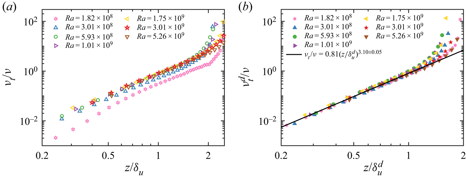
Figures 5(a) and 5(b) plot profiles of the normalised eddy viscosity  $\nu _t / \nu$ and
 $\nu _t^d / \nu$ in the laboratory frame and the dynamic frame, respectively. In the laboratory frame (figure 5a), the eddy viscosity profiles present no universal behaviour as the curves at low
 $Ra$ lie below the high
 $Ra$ cases. On the contrary, the profiles for
 $\nu _t^d / \nu$ in the dynamic frame (figure 5b) all collapse on a single master curve. A power-law fitting of all the data points within the viscous BL thickness, i.e.
 $z \le \delta _u^d$, yields
 \begin{equation} \nu_t^d / \nu = 0.81 {(z / \delta_u^d)}^{3.10 \pm 0.05}. \end{equation}
(a,b) Profiles of the normalised eddy viscosity  $\nu _t / \nu$ and
 $\nu _t^d / \nu$ as a function of the normalised wall distance
 $z / \delta _u$ and
 $z / \delta _u^d$ for different
 $Ra$ in (a) the laboratory frame and (b) the dynamic wall-shear frame. The solid line in panel (b) indicates the fitted power-law relation using all data points within the viscous BL thickness.

The scaling exponent  $\zeta = 3.10 \pm 0.05$ (
 $\nu _t^d \sim z^{\zeta }$) is close to those measured in the near-wall region of a quasi-2-D vertical thin disk (Xu et al. Reference Xu, Wang, He, Wang, Schumacher, Huang and Tong2021). This indicates that near the bottom plate, the effects of meandering/torsional/sloshing motions of the LSC are well-eliminated in the dynamic frame, and the viscous BL in 3-D and 2-D configurations seem to follow a universal dynamical process. The no-slip boundary condition and the continuity equation lead to
 $\langle u' w' \rangle _t = \partial \langle u' w' \rangle _t / \partial z = \partial ^2 \langle u' w' \rangle _t / \partial z^2 = 0$, which indicates that the leading order of the Reynolds shear stress is greater than or equal to three. Therefore, the concern scaling exponent being equal to three is not an exact theoretical result. Our result that the scaling exponent being
 $3.10\pm 0.05$ indicates that, within the experimental uncertainty, the higher-order terms (larger than three) also make a non-negligible contribution. We also remark that the scaling exponent for the eddy viscosity is close to that for the eddy thermal diffusivity (Shishkina et al. Reference Shishkina, Horn, Wagner and Ching2015; Schumacher et al. Reference Schumacher, Bandaru, Pandey and Scheel2016; Ching et al. Reference Ching, Leung, Zwirner and Shishkina2019).
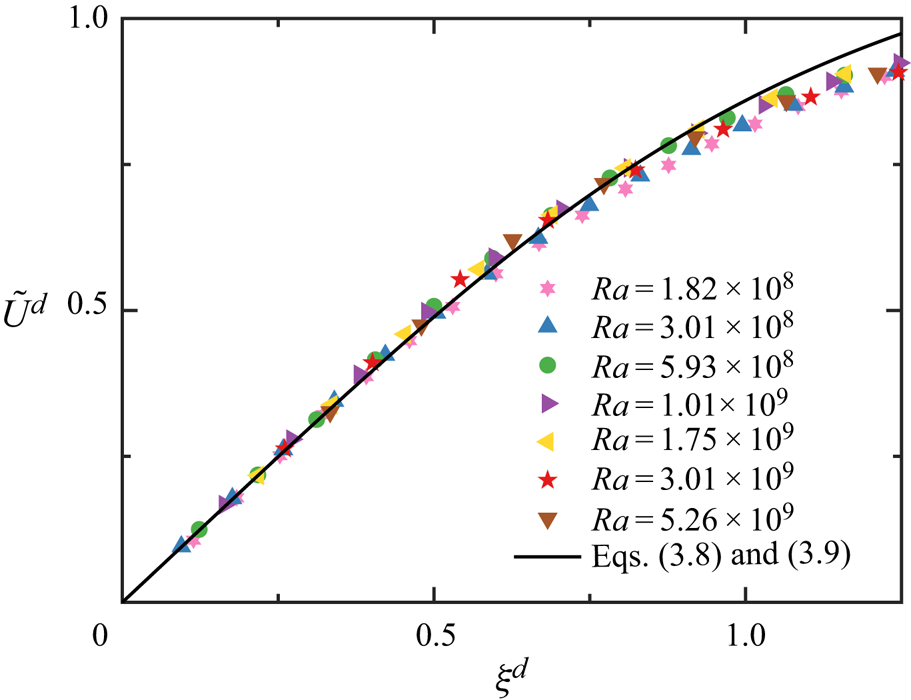
The formal solution of (3.6b) and (3.7b) in the dynamic wall-shear frame is
 \begin{equation} \tilde U^d(\xi^d) = \int_{0}^{\xi^d} \frac{1}{1 + \nu_t^d(s) / \nu} \,{\rm d}s, \end{equation}
wherein  $\xi ^d = z / \delta _u^d$ is the similarity variable, and
 $\tilde U^d = U^d / U_m^d$ is the normalised horizontal velocity. Therefore, the fitted eddy viscosity relation in (3.8) can be used to calculate the mean velocity profile via (3.9).
Figure 6 plots the profiles of the normalised velocity as a function of the normalised wall distance for different Rayleigh numbers in the dynamic frame. Since the eddy viscosity profiles do not overlap in the laboratory frame (see figure 5a), a corresponding general theoretical profile of the mean velocity cannot be obtained. The mean horizontal velocity profile following (3.8) and (3.9) is shown as the solid curve in figure 6, indicating a good agreement with the measured data points in the near-wall region. The deviation of the experimental data from the theoretical curve at positions far away from the wall may be partly attributed to the contributions by those neglected mean convection and pressure-gradient terms in (3.5). Additionally, considering the 3-D nature of the flow field in the cylindrical cell, the proposed reconstruction scheme based on the instantaneous wall-shear stress may be ineffective in the region far away from the wall.


3.3. The wall energy dissipation rate
The 3-D measurement of the viscous BL allows us to directly obtain the wall energy dissipation rate at the centre of the bottom plate  $\varepsilon _{w}$ as
 \begin{equation} \varepsilon_{w} = \nu \left[ \left( \left. \frac{\partial u}{\partial z} \right|_{z =0} \right)^2 + \left( \left. \frac{\partial v}{\partial z} \right|_{z =0} \right)^2 \right]. \end{equation}
The other terms in the velocity gradient tensor vanish at  $z = 0$ considering the no-slip boundary condition and the continuity equation.
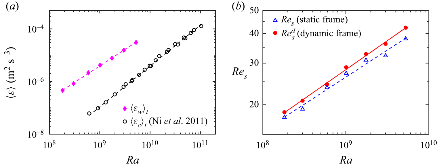
Figure 7(a) shows the mean wall dissipation rate  $\langle \varepsilon _w \rangle _t$ as a function of
 $Ra$. For reference, we plot in the same figure the indirectly measured mean dissipation rate at the cell centre
 $\langle \varepsilon _c \rangle _t$ (Ni et al. Reference Ni, Huang and Xia2011), as indicated by the black circles. The reference mean dissipation rate at the cell centre
 $\langle \varepsilon _c \rangle _t$ is corrected following
 $\langle \varepsilon _c \rangle _t \sim Pr^{1.15}$ to account for the variation of
 $Pr$ between 4.4 and 6.1 in Ni et al. (Reference Ni, Huang and Xia2011). For the parameter range explored in this study, the directly measured wall dissipation
 $\langle \varepsilon _w \rangle _t$ is over one order of magnitude larger than the centre reference
 $\langle \varepsilon _c \rangle _t$. The power-law scaling exponent on
 $Ra$ at the bottom plate (
 $\langle \varepsilon _{w} \rangle _t / (\nu ^3 H^{-4}) = 9.65 \times 10^{-2} Ra^{1.25 \pm 0.02}$) is smaller than that obtained in the cell centre (
 $\langle \varepsilon _c \rangle _t \sim Ra^{1.55 \pm 0.02}$). We also note that the measured scaling exponent of the wall dissipation is smaller than the value of 1.5 predicted by the Prandtl–Blasius laminar BL theory. We attribute this deviation to the strong fluctuations in the instantaneous wall-shear stress (see figure 2). The fitted lines for wall dissipation and the bulk dissipation intersect at
 $Ra = 2.2 \times 10^{14}$, which may be used to infer the transition to the ‘ultimate regime’ at which turbulent flow in the bulk starts to take over the entire convection cell and a new regime of heat transfer may emerge (Kraichnan Reference Kraichnan1962).
(a) The mean wall energy dissipation rate  $\langle \varepsilon _w \rangle _t$ as a function of
 $Ra$. The fitted power-law of the wall dissipation rate (magenta dashed line) is
 $\langle \varepsilon _{w} \rangle _t / (\nu ^3 H^{-4}) = 9.65 \times 10^{-2} Ra^{1.25 \pm 0.02}$. The mean dissipation rate by Ni et al. (Reference Ni, Huang and Xia2011) at the cell centre
 $\langle \varepsilon _c \rangle _t$ is included and corrected following
 $\langle \varepsilon _c \rangle _t \sim Pr^{1.15}$. (b) The shear Reynolds number
 $Re_s = \delta _u U_m / \nu$ and
 $Re_s^d = \delta _u^d U_m^d / \nu$ as a function of
 $Ra$. The fitted power-laws of the respective data are
 $Re_s = 0.229 Ra^{0.23 \pm 0.01}$ (blue dashed line) and
 $Re_s^d = 0.174 Ra^{0.24 \pm 0.01}$ (red solid line).

Another way to estimate the onset of ‘ultimate regime’ is based on the instability of the viscous BL. Figure 7(b) plots the shear Reynolds number  $Re_s = \delta _u U_m / \nu$ (
 $Re_s^d = \delta _u^d U_m^d / \nu$) as a function of
 $Ra$. The scaling exponents in two frames are similar, while the value of
 $Re_s^d$ in the dynamic frame is slightly larger than
 $Re_s$ in the laboratory frame. We tentatively estimate the onset
 $Ra_c$ at which the BL becomes unstable (i.e. the turbulent BL is expected to occur) following the critical Reynolds number
 $Re_s = 420$ (Landau & Lifschitz Reference Landau and Lifschitz1987; Ahlers et al. Reference Ahlers, Grossmann and Lohse2009). The resulting onset Rayleigh number is
 $Ra_c = 1.9 \times 10^{14}$ and
 $Ra_c = 6.1 \times 10^{13}$ in the static frame and the dynamic frame, respectively. We remark that these values are close to the preceding estimation of
 $Ra_c = 2.2 \times 10^{14}$ based on the bulk dissipation becoming dominant using the wall dissipation. He et al. (Reference He, Funfschilling, Nobach, Bodenschatz and Ahlers2012) reported a transition region covering
 $10^{13} \lesssim Ra_c \lesssim 5 \times 10^{14}$ and our estimates using both methods fall within this range. It is also worth mentioning that
 $Ra_c$ has been reported to be strongly dependent on the aspect ratio
 $\varGamma$ of the convection cell (Roche et al. Reference Roche, Gauthier, Kaiser and Salort2010; He, Bodenschatz & Ahlers Reference He, Bodenschatz and Ahlers2020; Ahlers et al. Reference Ahlers2022).
4. Conclusion and outlook
We have experimentally studied the viscous BL properties in turbulent RBC. High-resolution measurements of the velocity fields were conducted in two orthogonal vertical planes using two synchronised cameras in a cylindrical convection cell over the Rayleigh number range of  $1.82 \times 10^8 \le Ra \le 5.26 \times 10^9$ and the fixed Prandtl number
 $Pr = 4.34$. The extended p.d.f. of the wall-shear stress suggests that the horizontal velocity component in the mean LSC plane alone cannot fully characterise the instantaneous BL in the laboratory frame. We propose to reconstruct the BL profile in a dynamic frame based on the changing directions of the instantaneous wall-shear stress to eliminate the effects of complicated dynamics of the LSC. We examine the viscous BL properties and the eddy viscosity in the dynamic wall-shear frame and compared with those in the laboratory frame. In the dynamic frame, there exists a universal relationship
 $\nu _t^d / \nu = 0.81 (z / \delta _u^d) ^{3.10 \pm 0.05}$ describing the eddy viscosity with the wall distance at different Rayleigh numbers. In contrast, in the laboratory frame, the eddy viscosity profiles cannot be collapsed onto a master curve at low
 $Ra$. As far as the scaling with
 $Ra$ is concerned, the behaviours of the viscous BL thickness, the Reynolds number or the shear Reynolds number are the same in both frames within the experimental uncertainty. The scaling exponent of the viscous BL thickness with the Reynolds number is consistent with that of the Prandtl–Blasius BL. With the simultaneously measured viscous BL profiles in orthogonal vertical planes, we directly obtained the mean energy dissipation rate at the centre of the bottom plate
 $\langle \varepsilon _{w} \rangle _t$, which has much larger magnitude than the centre dissipation and follows the power-law scaling
 $\langle \varepsilon _{w} \rangle _t \sim Ra^{1.25}$. The observed wall dissipation scaling differs from the laminar BL theoretical prediction and provides an important constraint against which future theoretical models would be tested.
We would expect a strong positive correlation between the wall-shear stress direction and the direction of the LSC plane. The direction of the wall-shear stress, as a local property, presents locally intense fluctuations and is suitable for the reconstruction of the instantaneous velocity profile near the wall surface. In contrast, the LSC plane direction is a global property of the entire thermal convection system and reflects the coherent movements of large-scale structures. However, the direction of the LSC plane is not available in the present experimental set-up. We will study the relation between these two directions in our next work, in which the direction of the LSC plane will be measured by the azimuthally arranged thermistors close to the sidewall surface.
Previous studies indicate that, as the LSC moves in a more confined azimuthal range as a result of increasing the cell tilt angle, the power-law scaling exponent of the viscous BL thickness with  $Ra$ becomes smaller, i.e. larger in magnitude (Xin et al. Reference Xin, Xia and Tong1996; Lam et al. Reference Lam, Shang, Zhou and Xia2002; Wei & Xia Reference Wei and Xia2013). We do not yet have a clear explanation for the same scaling exponent in the dynamic and static frames in the present study in figure 3. A possible reason is the relatively large value of the tilt angle (
 $1.55^{\circ }$) applied in the present measurements. Within the experimental uncertainty, the scaling exponent of
 $\delta _u$ with
 $Ra$ remain unchanged at two tilt angles of
 $0.5^{\circ }$ and
 $1.0^{\circ }$, and reduces significantly at
 $2.0^{\circ }$ and
 $3.4^{\circ }$ (Wei & Xia Reference Wei and Xia2013). We will compare the dynamics of the wall-shear stress and the dynamics of the LSC plane (Zhang, Ding & Xia Reference Zhang, Ding and Xia2021; Zhang, Dong & Xia Reference Zhang, Dong and Xia2022) by measuring their directions simultaneously at various tilt angles in our next work.
Funding
We gratefully acknowledge support of this work by the National Natural Science Foundation of China (NSFC) (No. 12072144), the China Postdoctoral Science Foundation (no. 2021M701579) and the Center for Computational Science and Engineering of Southern University of Science and Technology.
Declaration of interests
The authors report no conflict of interest.