1 Introduction
Polymer drag reduction (
 $DR$
) in turbulent wall flows has been under intense investigation since the effect was first discovered by Toms (Reference Toms1948). It is now well documented that introducing only a few parts per million of long-chained polymer into a fluid can yield reductions in drag exceeding 60 % (up to near
 $80\,\%$
at low Reynolds number) relative to the drag produced in the flow of the solvent alone. Not surprisingly, this drag reduction is accompanied by modifications to statistical profiles, and accordingly the underlying structure of the turbulence. The relevant literature contains several important review articles, for example, Lumley (Reference Lumley1969), Berman (Reference Berman1978), White & Mungal (Reference White and Mungal2008), along with numerous journal articles documenting individual studies. Given this, a comprehensive literature review is neither practical nor warranted. Over the past decade, however, a relatively few number of issues central to characterizing the essential properties of the polymer drag reduction mechanisms, and the connections between the drag-reduced and canonical flows, have come to light. Those most relevant to the present contribution are now discussed in greater detail.
Herein we consider statistically stationary and fully developed turbulent channel flow with half-channel height
 $\unicode[STIX]{x1D6FF}$
. A defining characteristic of this flow, and of turbulent pipe and boundary layer flows as well, is the emergence of an interior domain over which the mean velocity profile approximates a logarithmic variation with distance from the wall. The accuracy of this logarithmic approximation increases as the Reynolds number becomes large. This behaviour is perhaps most clearly seen by plotting the inner-normalized streamwise velocity profile on semilogarithmic coordinates, i.e.
 $U^{+}=U/u_{\unicode[STIX]{x1D70F}}$
versus
 $y^{+}=yu_{\unicode[STIX]{x1D70F}}/\unicode[STIX]{x1D708}$
, where
 $u_{\unicode[STIX]{x1D70F}}=\sqrt{\unicode[STIX]{x1D70F}_{w}/\unicode[STIX]{x1D70C}}$
,
 $\unicode[STIX]{x1D70F}_{w}$
is the mean wall shear stress,
 $\unicode[STIX]{x1D70C}$
is the mass density,
 $y$
is the wall-normal direction, and
 $\unicode[STIX]{x1D708}$
is the kinematic viscosity. A generic property of a turbulent wall flow under the influence of a drag-reducing effect is that the inner-normalized mean velocity profile shifts upwards on the semilogarithmic graph previously mentioned, with the amount of
 $DR$
correlating with the magnitude of the upward shift. Here it is perhaps instructive to note that a similar, but opposite phenomenon occurs in rough-wall boundary layers, where the net increase in drag is generically associated with a downward profile shift.
The noted upward shift in the mean profile under polymer
 $DR$
directly connects to the descriptive model of Virk (Reference Virk1975). In this model, the net effect of the polymer generates a buffer layer of increased inner-normalized extent, beyond which the profile transitions to one that is parallel to the canonical logarithmic profile, i.e. parallel to
 $$\begin{eqnarray}\displaystyle U^{+}=\frac{1}{\unicode[STIX]{x1D705}}\ln (y^{+})+B, & & \displaystyle\end{eqnarray}$$
where
 $\unicode[STIX]{x1D705}$
is the von Kármán constant, and
 $B$
is a flow-dependent additive constant. Recent large-Reynolds-number quantifications indicate that
 $\unicode[STIX]{x1D705}\simeq 0.39$
for all three canonical turbulent wall flows (Marusic et al.
Reference Marusic, Monty, Hultmark and Smits2013). With increasing
 $DR$
, the transition point increasingly shifts to larger
 $y^{+}$
, and the logarithmic portion of the mean profile (with logarithmic slope
 $=\unicode[STIX]{x1D705}^{-1}$
) exhibits a concomitant upward shift. This behaviour occurs continuously throughout the so-called low drag reduction (LDR) regime (
 $DR\lesssim 40\,\%$
), and, according to the Virk model, also well into the high drag reduction (HDR) regime (
 $DR\gtrsim 40\,\%$
). In the models of Lumley (Reference Lumley1969) and Benzi et al. (Reference Benzi, Angelis, L’vov, Procaccia and Tiberkevich2006), the effective thickening of the buffer layer is described in terms of a position-dependent viscosity that increases with
 $y^{+}$
. At the end of the HDR regime, where maximum drag reduction (MDR) is attained, the profile shape terminates with the so-called ultimate profile. Here there is no transition to a logarithmic profile that is parallel to (1.1), and the profile appears to follow a logarithmic trend, but with a much larger profile slope.
While the Virk model retains a position of prevalence within polymer drag reduction thinking, recent studies cast doubt on important aspects of this description. Drawing upon a number of previous measurements, White, Dubief & Klewicki (Reference White, Dubief and Klewicki2012) provide evidence sufficient to hypothesize that the logarithmic slope of the mean profile begins to change from its canonical value in the LDR regime, and conclude that the characterization of the profile in the HDR regime and at MDR as logarithmic is not supported by a plateau in the plot of
 $y^{+}\text{d}U^{+}/\text{d}y^{+}$
versus
 $y^{+}$
. These results are also supported from the recent large-Reynolds-number data of Elbing et al. (Reference Elbing, Perlin, Dowling and Ceccio2013). More recently, White, Dubief & Klewicki (Reference White, Dubief and Klewicki2018) examined these and related issues in greater depth by considering flow properties associated with the structure of the mean momentum balance (MMB) in polymer drag-reduced channel flow. Here they used the FENE-P (Finite Elastic Nonlinear Extensibility-Peterlin) model-based direct numerical simulation (DNS) of Dubief et al. (Reference Dubief, White, Terrapon, Shaqfeh, Moin and Lele2004), Dubief, Terrapon & Soria (Reference Dubief, Terrapon and Soria2013) (
 $120\leqslant \unicode[STIX]{x1D6FF}^{+}\leqslant 300$
) and Thais et al. (Reference Thais, Tejada-Martinez, Gatski and Mompean2011), Thais, Mompean & Gatski (Reference Thais, Mompean and Gatski2013) (
 $395\leqslant \unicode[STIX]{x1D6FF}^{+}\leqslant 1000$
) to document the leading balance structure of the MMB for
 $30\,\%\leqslant DR\leqslant 62\,\%$
, where
 $\unicode[STIX]{x1D6FF}^{+}=\unicode[STIX]{x1D6FF}u_{\unicode[STIX]{x1D70F}}/\unicode[STIX]{x1D708}$
is the friction Reynolds number. Consistent with a thickened buffer layer, White et al. (Reference White, Dubief and Klewicki2018) found that for a fixed
 $\unicode[STIX]{x1D6FF}^{+}$
the leading-order inertial domain begins at larger
 $y^{+}$
with increasing
 $DR$
. They further provide evidence that, while the net effect of this is akin to an increased viscosity, the physical cause for this behaviour actually stems from a reduction of the Reynolds shear stress gradient owing to an attenuation of near-wall vorticity stretching and reorientation. Consistent with this, the motions associated with turbulent momentum transport are weakened and increase in size. Accordingly, the outward movement of the inertial domain restricts the formation of a region of logarithmic dependence, with the condition of high drag reduction associated with the eradication of an inertial sublayer. Owing in part to the relatively low Reynolds numbers of the White et al. (Reference White, Dubief and Klewicki2018) study, open questions remain regarding the mechanistic picture they surmised, as do details pertaining to the combined influences of
 $\unicode[STIX]{x1D6FF}^{+}$
and
 $DR$
. An additional open question is whether the same behaviour is observed in experiments as White et al. (Reference White, Dubief and Klewicki2018) documented using simulation results.
The aims of the present study seek to further investigate issues brought to light in the study of White et al. (Reference White, Dubief and Klewicki2018), as well as more deeply explore the properties of the flow on the inertial domain as a function of
 $DR$
and
 $\unicode[STIX]{x1D6FF}^{+}$
. Specifically, the present study experimentally elucidates the effects of Reynolds number for modest
 $DR$
(between
 $6.5\,\%$
and
 $26\,\%$
) over a range of
 $\unicode[STIX]{x1D6FF}^{+}$
beyond the DNS used in White et al. (Reference White, Dubief and Klewicki2018), and without the uncertainties associated with the veracity of the FENE-P model. High-fidelity data having a spatial resolution sufficient to accurately estimate velocity derivative profiles are necessary for addressing these aims. This is because, for example, the experimental reconstruction of the MMB requires accurate estimates of the wall-normal derivatives of the mean velocity profile. Recent efforts have successfully advanced this objective through the development of high-accuracy, high-density streamwise velocity measurements using the single-component version of molecular tagging velocimetry (1c-MTV) (Elsnab et al.
Reference Elsnab, Monty, White, Koochesfahani and Klewicki2017). In the present water channel flow experiments, 1c-MTV is used to generate instantaneous streamwise velocity profiles across the channel half-height, with each containing more than
 $850$
data points. With this capability, one can then explore a number of polymer
 $DR$
flow characteristics at levels of detail typically only associated with DNS. A primary objective here is to better understand polymer effects on the relevant momentum redistribution processes through analysis of the MMB and related properties. The present experiments are also designed to investigate the effect of the injected polymer concentration for varying Reynolds number, which has not been systematically explored previously.
In what follows, we first provide a brief description of the MMB analysis framework. We then describe experimental details pertaining to the channel flow facility and its polymer injection system, as well as the 1c-MTV measurement technique. The results of the polymer flow experiments, and their comparison to those without polymer, are then described and discussed. The paper closes with a discussion and conclusion section in which the ramifications of the present findings and further physical interpretations are provided.
1.1 Mean momentum equation analysis
Significant aspects of the present analysis connect to structural features associated with the mean dynamics. As such, we begin with the equation
 $$\begin{eqnarray}\displaystyle \underbrace{-\frac{1}{\unicode[STIX]{x1D70C}}\frac{\text{d}\overline{p}}{\text{d}x}}_{PG}+\underbrace{\unicode[STIX]{x1D708}\frac{\text{d}^{2}U}{\text{d}y^{2}}}_{VF}-\underbrace{\frac{\text{d}\overline{u^{\prime }v^{\prime }}}{\text{d}y}}_{TI}=0, & & \displaystyle\end{eqnarray}$$
which represents the time-averaged streamwise differential force balance for channel flow of a Newtonian fluid. In (1.2)
 $p$
is the pressure,
 $x$
is the streamwise direction,
 $\overline{u^{\prime }v^{\prime }}$
is the Reynolds stress,
 $PG$
is the pressure gradient,
 $VF$
is the mean viscous force and
 $TI$
is the turbulent inertia. For this paper,
 $U$
is the mean streamwise velocity, lower-case quantities with a superscript ‘prime’ are fluctuations, and an overbar represents an ensemble average.
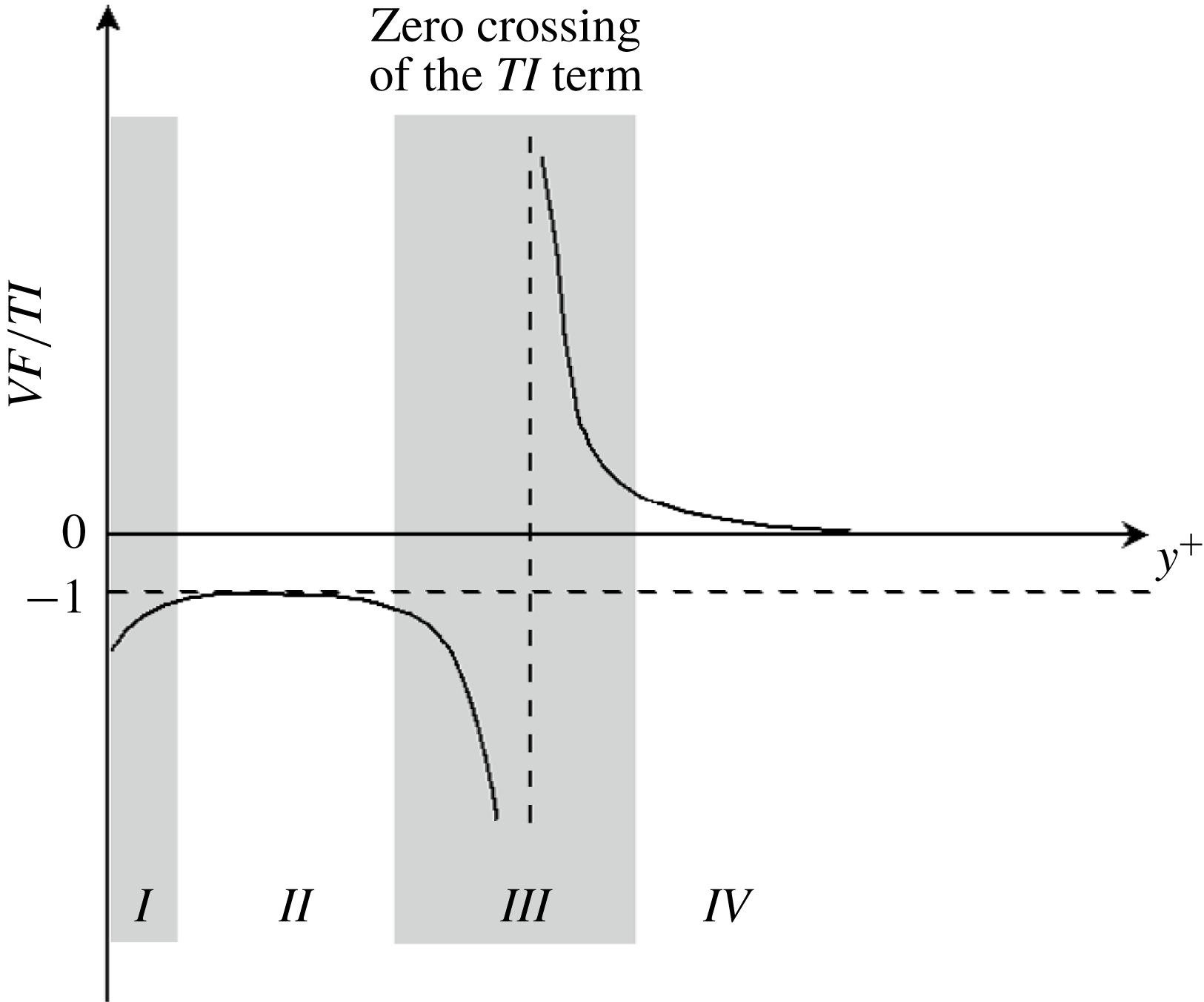
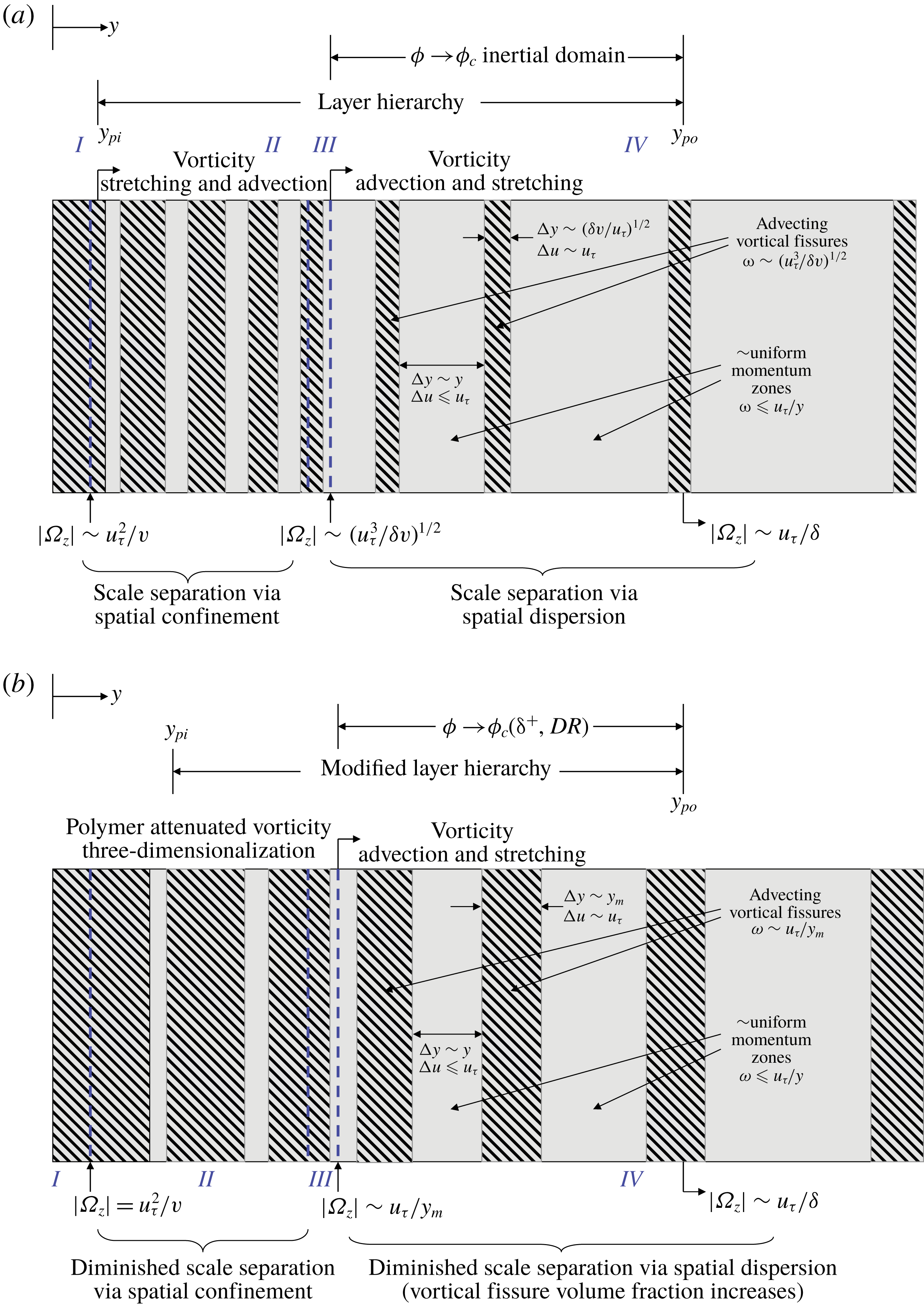
Consideration of how the terms balance in (1.2) yields the four-layer structure depicted in figure 1. This figure conveys how the ratio of viscous force to turbulent inertia changes across the half-channel (Wei et al.
Reference Wei, Fife, Klewicki and McMurtry2005). Here we note that while the Reynolds stress is the time-averaged turbulent momentum flux, it is the gradient (divergence) of this flux that appears in the mean force balance. In layer
 $I$
,
 $PG\approxeq VF$
. This is essentially the traditional viscous sublayer, and here the
 $TI$
term is negligible. In layer
 $II$
,
 $VF\approxeq TI$
, i.e. these stress gradients balance and the
 $PG$
term is subdominant. In layer
 $III$
, the
 $PG$
,
 $VF$
and
 $TI$
terms are all of the same order of magnitude. Across this layer, the leading balance of terms undergoes an exchange. This behaviour arises because the gradient of the Reynolds stress passes through zero. The balance exchange across layer
 $III$
culminates with the structure of layer
 $IV$
, where the leading balance is between the pressure gradient and turbulent inertia, and the
 $VF$
term is subdominant. When physically interpreted as a force, the
 $TI$
term acts as a momentum source on the wallward side of the maximum in the Reynolds stress, and a momentum sink beyond this maximum (Klewicki et al.
Reference Klewicki, Fife, Wei and McMurtry2007).
A sketch of the ratio of terms
 $VF/TI$
revealing the four-layer leading balance structure for turbulent channel flow (adapted from Wei et al.
Reference Wei, Fife, Klewicki and McMurtry2005).

The addition of polymer to the flow introduces an additional force-like term in (1.2). In inner-normalized form, the resulting equation is given by
 $$\begin{eqnarray}\displaystyle \underbrace{-\frac{1}{\unicode[STIX]{x1D6FF}^{+}}}_{PG}+\underbrace{\frac{\text{d}^{2}U^{+}}{\text{d}y^{+2}}}_{VF}-\underbrace{\frac{\text{d}\overline{u^{\prime }v^{\prime }}^{+}}{\text{d}y^{+}}}_{TI}+\underbrace{\frac{\text{d}\overline{\unicode[STIX]{x1D70F}_{xy}^{p}}^{+}}{\text{d}y^{+}}}_{GPS}=0, & & \displaystyle\end{eqnarray}$$
where
 $GPS$
is the gradient of the polymer stress,
 $y^{+}$
is the inner-normalized distance from the wall, and
 $\overline{\unicode[STIX]{x1D70F}_{xy}^{p}}^{+}$
denotes the polymer stress (
 $PS$
). For the Newtonian (
 $DR=0$
) case, the ratio
 $VF/TI$
provides a convenient way to expose the leading balance structure. For polymer
 $DR$
flows, a single ratio is insufficient owing to there being four terms in (1.3). Since the additional force-like term, the polymer stress gradient, is dynamically similar to the Reynolds stress gradient, the sum of the Reynolds and polymer shear stress is represented as a combined apparent stress (White et al.
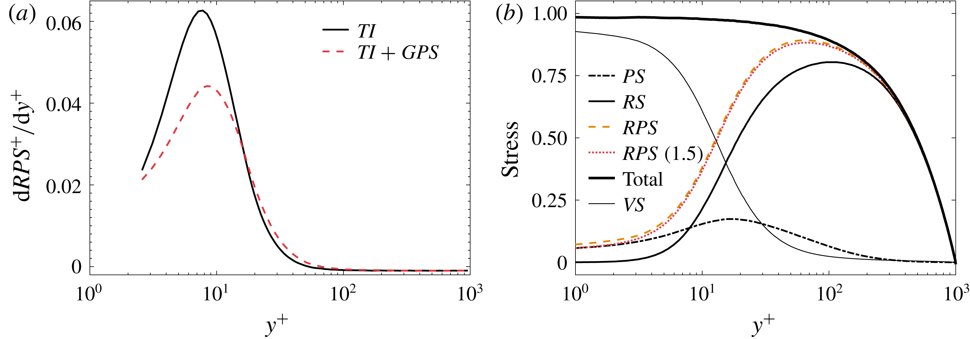
Reference White, Dubief and Klewicki2018). The viscoelastic DNS of Thais et al. (Reference Thais, Mompean and Gatski2013) at
 $\unicode[STIX]{x1D6FF}^{+}=1000$
is shown in figure 2(a). These data indicate that the gradient of the polymer stress has properties that are qualitatively similar to the
 $TI$
term in Newtonian flows. The skin friction drag in this flow is approximately
 $30\,\%$
less than a Newtonian flow at the same
 $\unicode[STIX]{x1D6FF}^{+}$
. The analysis of White et al. (Reference White, Dubief and Klewicki2018) demonstrated that the ratio
 $VF/(TI+GPS)$
provides a useful means to reveal the structure associated with the magnitude ordering of terms in polymer
 $DR$
channel flow.
The mean viscous force is determined from the velocity profile, and thus requires high-resolution velocity profile data that are twice differentiable. The Reynolds stress is then calculated by integrating the mean momentum equation and applying boundary conditions, with the resulting familiar equation for the
 $DR=0$
flow given by
 $$\begin{eqnarray}\displaystyle -\overline{u^{\prime }v^{\prime }}^{+}=1-\frac{y^{+}}{\unicode[STIX]{x1D6FF}^{+}}-\frac{\text{d}U^{+}}{\text{d}y^{+}}. & & \displaystyle\end{eqnarray}$$
The corresponding relation for polymer flows is found by integrating (1.3), and is given by
 $$\begin{eqnarray}\displaystyle \underbrace{-\overline{u^{\prime }v^{\prime }}^{+}+\overline{\unicode[STIX]{x1D70F}_{xy}^{p}}^{+}}_{RPS}=1-\frac{y^{+}}{\unicode[STIX]{x1D6FF}^{+}}-\frac{\text{d}U^{+}}{\text{d}y^{+}}. & & \displaystyle\end{eqnarray}$$
In (1.5),
 $RPS$
is the sum of the Reynolds and polymer stress. Figure 2(b) supports the validity of using this method to obtain the
 $RPS$
, as the balance of (1.5) is satisfied to very high accuracy. Herein, the total stress is calculated as the sum of the viscous
 $(VS)$
, Reynolds (
 $RS$
) and polymer (
 $PS$
) stress. Note also that at the wall the inner-normalized mean velocity gradient does not exactly equal
 $1$
owing to the influence of the polymer stress.
(a) Reynolds stress gradient at
 $\unicode[STIX]{x1D6FF}^{+}=1000,DR=0$
(solid line) and
 $TI+GPS$
at
 $\unicode[STIX]{x1D6FF}^{+}=1000,DR=30\,\%$
(dash–dot line). (b) Terms in (1.5) for polymer flow at
 $\unicode[STIX]{x1D6FF}^{+}=1000$
with
 $DR=30\,\%$
. Viscoelastic DNS data are from Thais et al. (Reference Thais, Mompean and Gatski2013).

2 Experiment description
2.1 Facility
The present experiments employed a rectangular water channel depicted schematically in figure 3. The test section dimensions of this facility are 60 mm
 $\times$
750 mm
 $\times$
9000 mm (
 $H\times W\times L$
), where
 $H=2\unicode[STIX]{x1D6FF}$
is the channel height,
 $W$
is the channel width (span) and
 $L$
is the length. The horizontal surfaces of the test section are made of machined cast aluminium plates (flat within
 $0.127~\unicode[STIX]{x03BC}\text{m}$
with a maximum surface roughness of
 $0.5~\unicode[STIX]{x03BC}\text{m}$
), while the sidewalls are made of stainless steel. Upstream of the test section, the flow passes through a bank of three screens, and then into a 6.66:1 contraction. Wall pressure taps, 1 mm in diameter, located at
 $x/H=15$
,
 $31.7$
,
 $48.3$
,
 $65$
,
 $81.7$
and
 $98.3$
are used to measure the pressure drop. A downstream pressure port located at
 $x/H=131.7$
is used as the reference pressure for the six
 $\unicode[STIX]{x0394}p$
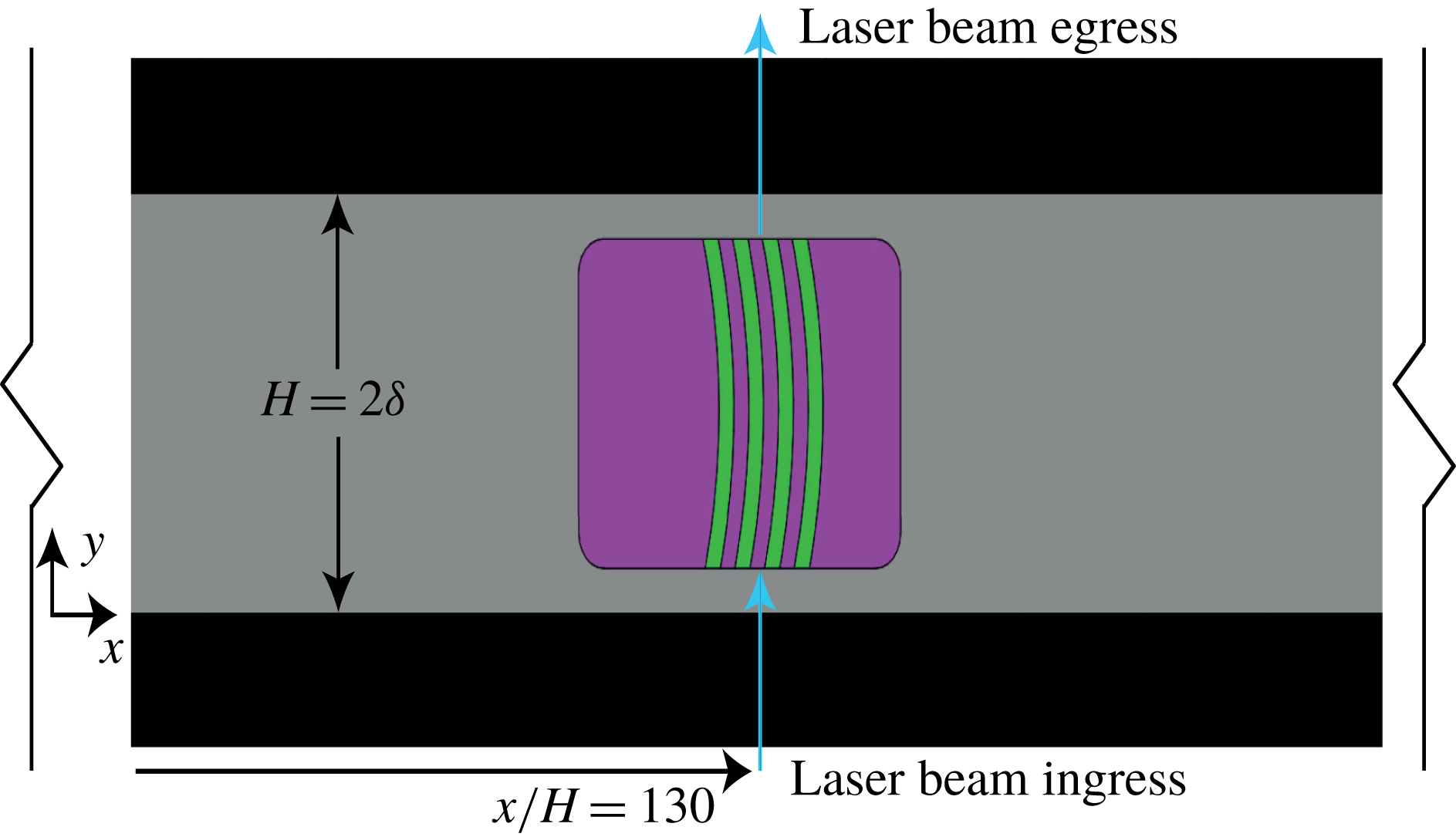
sensors. Fused silica windows made flush with the interior surfaces of the channel allow laser and camera access. As depicted in figure 4, these windows are located approximately
 $130H$
downstream of the test section inlet. A centrifugal pump and a variable frequency controller are used to produce the constant mass flow rate conditions explored. The volumetric flow rate is measured using a turbine style flow meter. Further details regarding the flow channel are given in Elsnab et al. (Reference Elsnab, Monty, White, Koochesfahani and Klewicki2017).
Owing to its finite width, the present channel only approximates the analytical ideal of an infinitely wide channel. This issue is potentially significant to estimating the friction velocity from the measured pressure drop, as well as relative to properly interpreting flow modifications associated with polymer effects. In this regard, Monty & Chong (Reference Monty and Chong2009) showed that data from a channel of aspect ratio equalling
 $11.7$
exhibited excellent agreement with DNS data at similar
 $\unicode[STIX]{x1D6FF}^{+}$
. The present aspect ratio of
 $12.5$
is believed to approximate two-dimensional channel flow with high accuracy, and similar aspect ratios have been used in polymer drag reduction studies (Wei & Willmarth Reference Wei and Willmarth1992; Warholic, Massah & Hanratty Reference Warholic, Massah and Hanratty1999).
Schematic of the experimental facility.
 $S_{i}$
denote the screen locations.

Schematic of the portion of the facility where the MTV measurements were acquired. Flow is from left to right and the green lines represent a view of the deformed image of the molecularly tagged lines. Note that the camera is angled
 $1^{\circ }$
downwards so that the near-wall region is captured. Adapted from Elsnab et al. (Reference Elsnab, Monty, White, Koochesfahani and Klewicki2017).

The friction velocity is the fundamental scaling parameter for wall-bounded flows. For non-canonical flows, determining the friction velocity is more difficult than the Newtonian channel flow case where
 $u_{\unicode[STIX]{x1D70F}}$
is determined from the linear pressure drop data in the fully developed region. For polymer-influenced channel flows with wall injection, the drag reduction is not exactly constant in the streamwise direction (Tidederman, Luchik & Bogard Reference Tidederman, Luchik and Bogard1985). Therefore, the flow is not technically ‘fully developed’. There is, however, a region where the
 $DR$
is nearly constant (1 %–4 % variation) over more than
 $50H$
upstream of the MTV measurement location, and remains constant for the duration of the drag-reduced MTV data acquisition. The friction velocity is first evaluated from the pressure drop measurements across the test section where the drag reduction is approximately constant. A linear curve fit of the pressure data over the region where the
 $DR$
is nearly constant is used to determine the pressure gradient, and hence
 $u_{\unicode[STIX]{x1D70F}}$
. Since the drag reduction over this region varies by 1 %–4 %, the friction velocity will vary by approximately 1 %–3 %. Note that the variation in the friction velocity is due to the slow streamwise development of the flow in this region.
The more ideal scenario to minimize the influence of flow development is to acquire a local measure of the friction velocity at the MTV measurement location. Owing to the high spatial resolution of the MTV (more than 850 data points per wall-normal profile with spatial resolution similar to DNS data (Elsnab et al.
Reference Elsnab, Monty, White, Koochesfahani and Klewicki2017)) a fitting method was employed. Specifically, both experimental and viscoelastic DNS data (Dubief et al.
Reference Dubief, White, Terrapon, Shaqfeh, Moin and Lele2004; Hou, Somandepalli & Mungal Reference Hou, Somandepalli and Mungal2008; Somandepalli, Hou & Mungal Reference Somandepalli, Hou and Mungal2010; Thais et al.
Reference Thais, Mompean and Gatski2013; Owolabi, Dennis & Poole Reference Owolabi, Dennis and Poole2017) show that the inner-normalized velocity profile in
 $DR$
flow matches the Newtonian profile for
 $y^{+}\leqslant 11.6$
. Given this, to determine
 $u_{\unicode[STIX]{x1D70F}}$
, the inner-normalized velocity is forced to match the Newtonian profile for
 $y^{+}\leqslant 11.6$
. Typically, 3–5 points were used for the fit, with the first point starting at
 $y^{+}=6{-}8$
. The friction velocity found using the fitting method was within
 $({\approx}0.5\,\%{-}3\,\%)$
of the friction velocity determined from the pressure drop measurements. The main advantage of using the fitting method is the reduction of data scatter. The uncertainty in the Newtonian values for
 $u_{\unicode[STIX]{x1D70F}}$
is approximately 1 %–2 %, as assessed using the method described by Moffat (Reference Moffat1988).
For the polymer-influenced flows, the viscosity of water was used since there is negligible difference between the viscosity of water and the viscosity of a
 $5$
wppm polymer solution (the homogeneous concentration of polymer at the MTV measurement station). Fluid temperature was measured using shielded T-type thermocouples at the inlet and outlet of the test section. Dynamic viscosity and fluid density as a function of temperature were obtained using correlations provided by Nagashima (Reference Nagashima1977) and Hyland & Wexler (Reference Hyland and Wexler1980), respectively.
2.2 Polymer mixing and injection manifold
Polyethylene oxide (PEO) with a molecular weight
 $(M_{w})$
of
 $4$
million was used as the polymer in the present experiments. A polymer slurry was made using a 50 : 50 by volume mixture of polyethylene glycol (PEG) and PEO. Note that PEO is insoluble in PEG, and thus when mixed, a slurry of PEG and suspended PEO powder is formed. The benefit here is that aggregation of the PEO, which occurs due to swelling when hydrated rapidly, can be greatly reduced by slowly mixing the slurry into solution. The aggregation is common and difficult to prevent when mixing PEO powder directly into water. The concentration of PEG in the final solution is so low it has a negligible effect on the physical properties of the final
 $30$
l solution. The PEO/PEG slurry and MTV solution, described in § 2.4, were mixed in a
 $30$
l modified pool filtration system pressure vessel. Here the PEO/PEG slurry was slowly introduced into the mixing vessel by dripping it down a plastic cone, while the MTV solution was injected from a shower nozzle. The overall solution was then gently stirred and allowed to hydrate for 24 h.
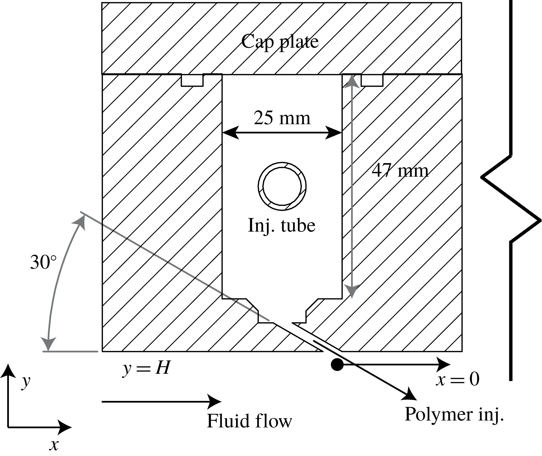
The polymer solution was introduced at the inlet to the test section using slots in the top and bottom surfaces. This involved using two manifolds and two mixing vessels. The 2 mm injection slots span the entire channel width and have an orientation of
 $30^{\circ }$
to the flow direction as depicted in figure 5. Polymer was introduced into the manifold through 10 mm diameter stainless steel tubes, and uniformly distributed via
 $161$
holes of 0.95 mm diameter. To promote uniform distribution in the manifold, these holes were logarithmically spaced near the vertical channel walls, and linearly spaced near the channel centre
 $z/H=\pm 7$
. Dry nitrogen was used to pressurize the injection system. A piping tee was used to direct the polymer solution flow to each manifold.
The polymer injection volume flow rate per unit width, as quantified by two magnetic flow rate sensors, was nominally matched to the lower portion of the viscous wall layer,
 $Q_{s}=67.3\unicode[STIX]{x1D708}$
, where
 $\unicode[STIX]{x1D708}$
is the kinematic viscosity of water at
 $18\,^{\circ }\text{C}$
(Wu & Tulin Reference Wu and Tulin1972). The region of interest was set at
 $y^{+}<11.6$
, and then to minimize the disturbance, the actual injection flow rate was set to
 $Q_{i}/Q_{s}\approxeq 0.75$
(Walker, Tiederman & Luchik Reference Walker, Tiederman and Luchik1986). The additional mass flow from the polymer injection was drained from the facility through
 $20$
mm diameter tubing located at the fill point of the facility. The fill point is open to the atmosphere and is located two metres above the test section. Draining off the added fluid ensured that the hydrostatic pressure in the system remained constant.
Schematic of the polymer solution injection manifold. There are two such manifolds, one attached to the top surface of the channel and other on the bottom surface.

2.3 Homogeneous versus wall injection
In the results section, trends based upon homogeneous polymer concentration are compared with those obtained with wall injection. It is therefore important to provide an estimation on the level of polymer homogeneity across the channel height. The evolution of channel flow with wall injection of drag-reducing polymer is similar to that reported in boundary layer studies with wall injection (e.g. Hou et al.
Reference Hou, Somandepalli and Mungal2008; Winkel et al.
Reference Winkel, Oweis, Vanapalli, Dowling, Perlin, Solomon and Ceccio2009; Somandepalli et al.
Reference Somandepalli, Hou and Mungal2010; Elbing et al.
Reference Elbing, Perlin, Dowling and Ceccio2013) and in channel flow studies with wall injection by Tidederman et al. (Reference Tidederman, Luchik and Bogard1985), Walker et al. (Reference Walker, Tiederman and Luchik1986), Luchik & Tiederman (Reference Luchik and Tiederman1988) and Walker & Tiederman (Reference Walker and Tiederman1990). The study by Somandepalli et al. (Reference Somandepalli, Hou and Mungal2010) indicated that the polymer was homogeneous across approximately
 $42\,\%$
of the boundary layer thickness for injected polymer concentrations up to
 $500$
wppm at
 $50x/\unicode[STIX]{x1D6FF}_{99}$
downstream of the injection location, where
 $\unicode[STIX]{x1D6FF}_{99}$
is the local boundary layer thickness. For high
 $Q_{i}/Q_{s}$
(
 ${\approx}\,2{-}10$
) the mixing of the polymer across the channel has been found to be slower than low
 $Q_{i}/Q_{s}$
(Winkel et al.
Reference Winkel, Oweis, Vanapalli, Dowling, Perlin, Solomon and Ceccio2009; Elbing et al.
Reference Elbing, Perlin, Dowling and Ceccio2013). This is one reason why low
 $Q_{i}/Q_{s}$
is used in the present study. Hou et al. (Reference Hou, Somandepalli and Mungal2008) reported that a comparison between homogeneous concentration channel flow at MDR and an inhomogeneous concentration turbulent boundary layer at MDR indicated that the former shows a polymer stress contribution of
 $60\,\%$
, while the latter shows
 $25\,\%$
. This appears to be the fundamental difference associated with an inhomogeneous versus a homogeneous distribution of polymer at MDR. This is attributed to the modification in the Reynolds stress profiles. In the inhomogeneous case, the Reynolds stress away from the wall will play a lesser role in the overall
 $DR$
. In the homogeneous channel case, the Reynolds stress is reduced across the entire channel height, with the primary reduction close to the wall being responsible for the dominant
 $DR$
effect.
For channel flow studies, Walker et al. (Reference Walker, Tiederman and Luchik1986) indicated that nearly constant drag reduction was obtained after
 $50$
channel heights downstream of the injector. This result was used by Luchik & Tiederman (Reference Luchik and Tiederman1988) in their channel flow study with wall injection. Walker & Tiederman (Reference Walker and Tiederman1989) reported that
 $3.33H$
downstream of the injection location, the near-wall concentration was reduced from
 $0.75\,\%$
to
 $0.25\,\%$
of the injection concentration. Wei & Willmarth (Reference Wei and Willmarth1992) injected polymer in the settling chamber located before the contraction. They reported that for
 $500\leqslant C_{i}\leqslant 2000$
wppm there were no issues in obtaining a homogeneous polymer concentration across the channel height. Kim et al. (Reference Kim, Islam, Shen, Sirviente and Solomon2004) reported that for
 $C_{i}>3000$
wppm, the polymer was not homogeneous at the channel centreline at a streamwise distance of
 $76H$
from injection.
The aforementioned results indicate that in the present experiments (with low
 $Q_{i}/Q_{s}<1$
and
 $C_{i}<2000$
wppm) the polymer is approximately homogeneously mixed across the channel height at the MTV measurement station located
 $130H$
downstream from the injection location. These results also indicate that there is sufficient streamwise distance for the profile to become quasi-fully developed. Therefore, the present results are deemed relevant to homogeneous channel flow as well.
2.4 Molecular tagging velocimetry
Molecular tagging velocimetry was used to measure the instantaneous streamwise velocity profiles at high resolution. This technique involves the Lagrangian tracking of molecularly tagged regions of the flow. In this case, the single-component version of MTV that uses a series of narrow lines is used to obtain the streamwise velocity. Ultraviolet laser light is used to excite the fluid molecules that are imaged at an initial time,
 $t_{o}$
, and subsequently at a delayed time,
 $t_{o}+\unicode[STIX]{x0394}t$
, within the lifetime of the tracer (described below). Here
 $\unicode[STIX]{x0394}t$
is the time delay between the two successive images. In processing, the velocity field is determined from the measured Lagrangian displacement of the tagged molecules between two successive images.
While the high spatial resolution afforded by 1c-MTV facilitates the accurate estimation of derivatives, the high data density renders derivative quantities especially sensitive to measurement noise. The recent study by Elsnab et al. (Reference Elsnab, Monty, White, Koochesfahani and Klewicki2017) demonstrates that the pre- and postprocessing steps employed in the present implementation produce high-resolution mean profiles that are twice differentiable. This capability allows for the reconstruction of the MMB.
The MTV solution employed is 1-BrNp
 $\cdot$
M
 $\unicode[STIX]{x1D6FD}$
-CD
 $\cdot$
ROH (Koochesfahani & Nocera Reference Koochesfahani and Nocera2007). The concentration of the individual constituents making up the MTV solution is
 $2\times 10^{-4}~\text{M}$
for the cyclodextrin, M
 $\unicode[STIX]{x1D6FD}$
-CD,
 ${\sim}10^{-5}~\text{M}$
for the lumophore, 1-BrNP, and
 $0.05$
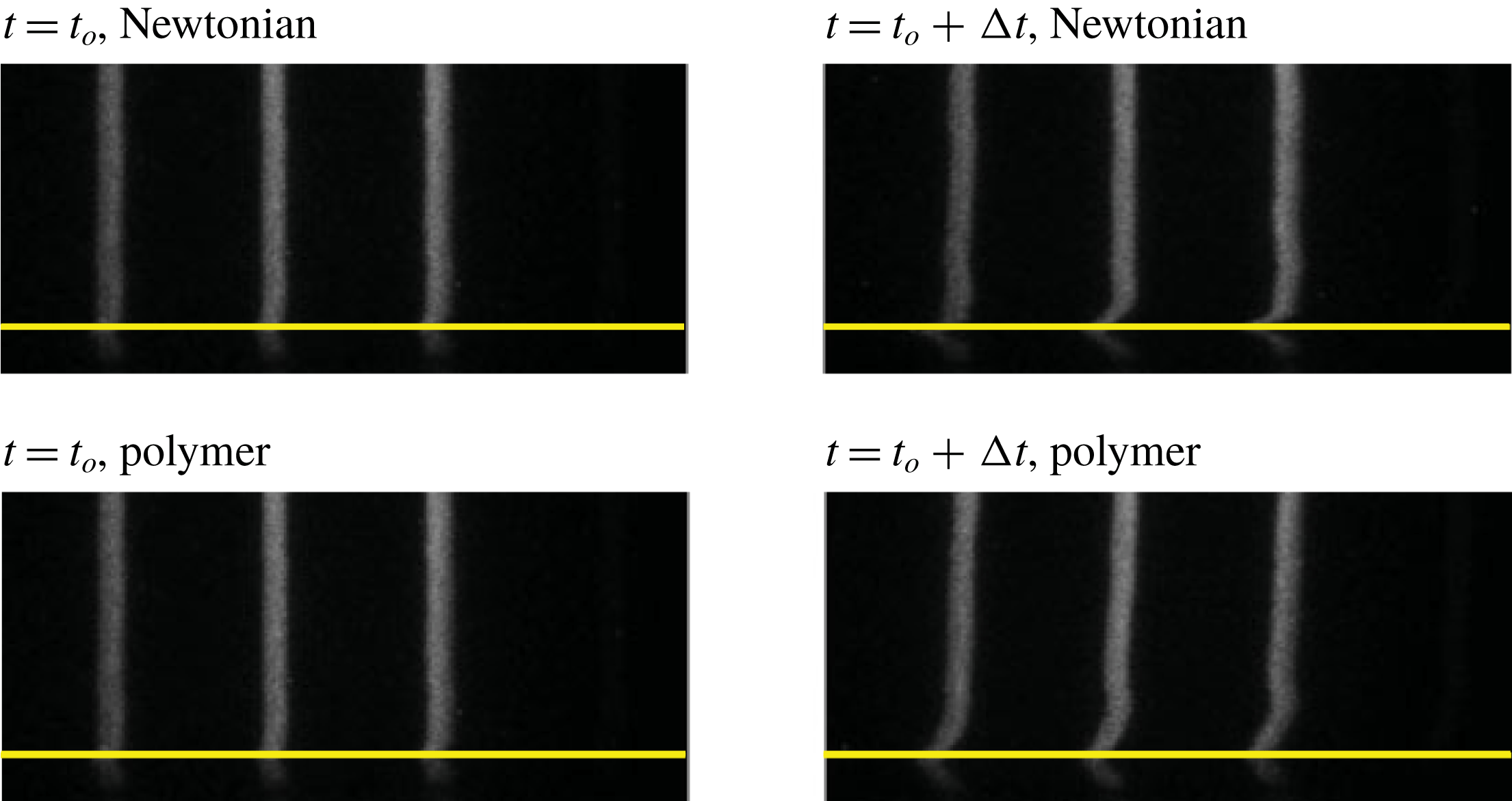
M for the alcohol concentration, ROH (Koochesfahani & Nocera Reference Koochesfahani and Nocera2007). For this study, cyclohexanol was used as the ROH. The MTV solution is homogeneously mixed within the entire volume of fluid in the channel, and homogeneously mixed at the same concentration in the injected polymer slurry. Thus, as evidenced in figure 6, there is no observable effect of polymer on the raw image quality. Variations in density or viscosity of the carrier fluid (water) were not detectable. The photosensitive molecules in the fluid were tagged using the fourth harmonic (266 nm) of a Spectra Physics Pro-350 Nd:YAG laser. The resulting pattern consisted of a series of streamwise-spaced lines that each extended across the channel height. These lines were formed using a precision array of 0.75 mm diameter pinholes having a 4 mm pitch. The MTV images were captured using a 1024
 $\times$
1024 pixel Princeton Instruments PI:MAX4 ICCD camera, with pixel dimensions of
 $12.8\times 12.8~\unicode[STIX]{x03BC}\text{m}$
. Between
 $2000$
and
 $2500$
image pairs were acquired at a rate of 5 Hz, with 3–4 laser lines per image. The field of view in the wall-normal direction was from
 $y=0~\text{mm}$
to
 $y=33~\text{ mm}$
. The time delay between successive interrogations ranged from
 $556~\unicode[STIX]{x03BC}\text{s}$
to
 $2619~\unicode[STIX]{x03BC}\text{s}$
, with an exposure time for the
 $t_{o}$
and
 $t_{o}+\unicode[STIX]{x0394}t$
images of
 $50~\unicode[STIX]{x03BC}\text{s}$
and
 $75~\unicode[STIX]{x03BC}\text{s}$
, respectively. To remove laser reflections,
 $t_{o}$
images were acquired
 $5~\unicode[STIX]{x03BC}\text{s}$
after laser emission. Further details regarding the experimental procedures employed are given in Elsnab et al. (Reference Elsnab, Monty, White, Koochesfahani and Klewicki2017).
Instantaneous images of
 $t_{o}$
and
 $t_{o}+\unicode[STIX]{x0394}t$
MTV lines. The fluid flow is from left to right. The solid yellow line represents the wall location, and only
 $1/5$
of the image height is presented. For the polymer case, the injection concentration is
 $C_{i}=2000~\text{wppm}$
.

2.5 Data reduction
Postacquisition image preprocessing utilized a spatial smoothing step that incorporates a median filter with five streamwise data points at each wall-normal location (Caso & Bohl Reference Caso and Bohl2014). Each pixel in the MTV images was then corrected according to
 $$\begin{eqnarray}\displaystyle I_{C}(x_{i},y_{j})=\frac{I(x_{i},y_{j})-DF(x_{i},y_{j})}{FF(x_{i},y_{j})-DF(x_{i},y_{j})}, & & \displaystyle\end{eqnarray}$$
where
 $I_{C}$
is the normalized image,
 $I$
is the instantaneous image,
 $DF$
is the darkfield image, and
 $FF$
is the flatfield image. The flatfield image is captured at the same intensifier gain as the MTV images.
The instantaneous
 $t_{o}$
images are cross-correlated with their respective
 $t_{o}+\unicode[STIX]{x0394}t$
image. An FFT-based cross-correlation at each wall-normal pixel location was used to determine the bulk displacement. Refinement to subpixel displacement was then determined by curve-fitting a second-order polynomial through the peak in the correlation distribution. Following the method outlined by Bohl (Reference Bohl2002), the
 $95\,\%$
measurement error for the camera was determined to be
 $0.3$
pixel. The measurement error for the camera is determined by imaging a static target that consists of white vertical lines separated by black lines. The line width of the white lines is set to approximately that of the MTV images, around
 $18$
pixel. Cross-correlating the static image allows for the measurement error to be determined. Ideally, this analysis should yield zero displacement. By cross-correlating over 100 images, the distribution of errors about the perfect (zero displacement) condition is obtained. From this, the estimated subpixel accuracy of the mean displacement is
 $0.15/\sqrt{N}$
pixel, where
 $N$
is the number of profiles used in the average. The corresponding uncertainty in the mean centreline velocity was
 $0.25\,\%$
. Each measured profile contains approximately
 $880$
data points. The methods to determine the wall-position and the pixel-to-physical space conversion are described in Elsnab et al. (Reference Elsnab, Monty, White, Koochesfahani and Klewicki2017).
As described in Elsnab et al. (Reference Elsnab, Monty, White, Koochesfahani and Klewicki2017), MTV measurements of the streamwise velocity intensity are subject to spatial filtering effects. The attenuation in these signals stems from the finite MTV line width in the spanwise direction. Here the MTV measurements exhibit an effect similar to a single-element hot-wire sensor that is also susceptible to spatial averaging owing to its finite spanwise length. This attenuation effect is distinct from the volumetric attenuation typically experienced by particle image velocimetry or laser Doppler velocimetry measurements, and can be corrected using the technique described by Lee et al. (Reference Lee, Kevin and Hutchins2016). Following Elsnab et al. (Reference Elsnab, Monty, White, Koochesfahani and Klewicki2017), when the estimated light-sheet thickness (full-width at half-maximum intensity) is used as the characteristic sensor length (0.6 mm), the present corrected MTV results for Newtonian flow closely adhere to those obtained via DNS. The length scale associated with the attenuation can be argued to be appropriate if it does not change with Reynolds number. This condition was determined to hold for the present data over the range
 $600<\unicode[STIX]{x1D6FF}^{+}<1800$
(Elsnab et al.
Reference Elsnab, Monty, White, Koochesfahani and Klewicki2017).
3 Results
3.1 Parameter space
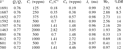
The parameter space investigated in the present experiments is described in table 1. The friction Reynolds numbers,
 $\unicode[STIX]{x1D6FF}^{+}$
, ranges from 580 to 1690. Note that
 $\unicode[STIX]{x1D6FF}^{+}$
for the Newtonian flows were
 $\approxeq 650$
,
 $975$
and
 $1800$
. The ratio
 $Q_{i}/Q_{s}$
refers to the relative flow rate of the injected fluid to the wall layer flow rate, as discussed above. Here
 $C_{i}$
is the concentration of the injected fluid, and
 $C_{h}$
is the bulk concentration in the channel. The bulk concentration assumes a homogeneous mixture and is determined by using the measured volumetric flow rate obtained from a turbine style flow meter. The estimated drag reduction for each scenario is also listed. The friction Weissenberg number,
 $We_{\unicode[STIX]{x1D70F}}$
, defined as the ratio of the polymer time scale to the flow time scale is given by
 $$\begin{eqnarray}\displaystyle We_{\unicode[STIX]{x1D70F}}=\frac{\unicode[STIX]{x1D706}u_{\unicode[STIX]{x1D70F}}^{2}}{\unicode[STIX]{x1D708}_{0}}, & & \displaystyle\end{eqnarray}$$
where
 $\unicode[STIX]{x1D706}$
is the polymer relaxation time and
 $\unicode[STIX]{x1D708}_{0}$
is the zero shear rate kinematic viscosity of the solution. In table 1,
 $\unicode[STIX]{x1D706}$
is determined using the Rouse–Zimm theory and is approximated as
 $$\begin{eqnarray}\displaystyle \unicode[STIX]{x1D706}_{z}=0.422\frac{[\unicode[STIX]{x1D702}]M_{w}\unicode[STIX]{x1D707}_{s}}{N_{A}k_{B}T}, & & \displaystyle\end{eqnarray}$$
where
 $[\unicode[STIX]{x1D702}]=0.072M_{w}^{0.65}$
is the intrinsic viscosity of the PEO solution,
 $\unicode[STIX]{x1D707}_{s}$
is the solvent dynamic viscosity,
 $N_{A}$
is Avogadro’s number,
 $k_{B}$
is the Boltzmann constant, and
 $T$
is the temperature (Zimm Reference Zimm1956).
In the present study, depending on
 $C_{i}$
, the solution concentration from the point of injection to the MTV measurement station will range from semidilute
 $(C^{\ast }<C<C_{e})$
to dilute
 $(C<C^{\ast })$
, where
 $C^{\ast }$
is the critical overlap concentration and
 $C_{e}$
is the entanglement concentration beyond which topological interactions play a role. Correlations correcting for the affect of concentration on
 $\unicode[STIX]{x1D706}$
in the dilute regime can be found in Tirtaatmadja, McKinley & Cooper-White (Reference Tirtaatmadja, McKinley and Cooper-White2006). Note that at the MTV measurement station
 $C\approx C_{h}$
and the Zimm relaxation time provides a suitable measure of the polymer relation time. White, Somandepalli & Mungal (Reference White, Somandepalli and Mungal2004) reported a polydispersity of 1.45 for the same polymer molecular weight as used in the present study. It is therefore likely that the polymer in the present study has a similar polydispersity, which means there exists a distribution of molecular weights and, consequently, a single
 $We_{\unicode[STIX]{x1D70F}}$
is effectively a representative measure of the viscoelastic effects of the solution.
Experimental parameters for the polymer drag-reduced flows investigated.

3.2 Potential effects associated with the injection process
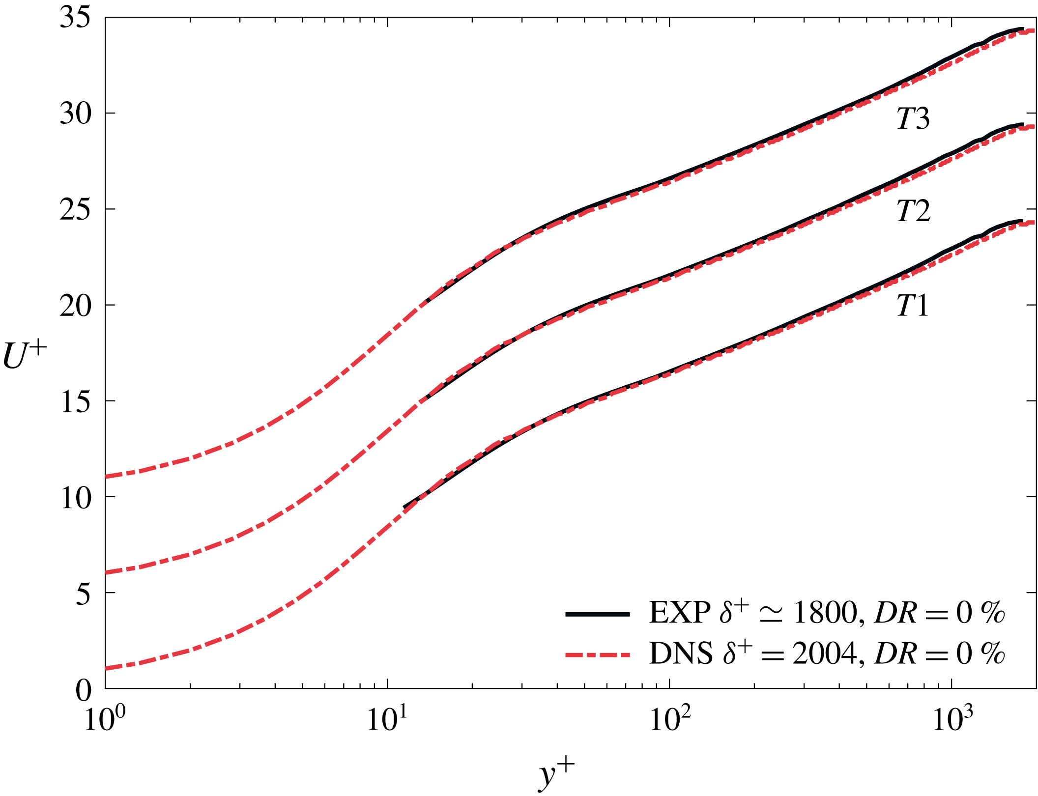
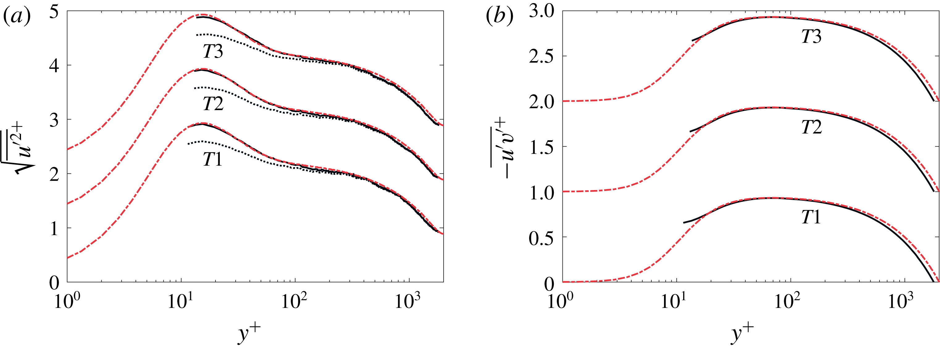
Significant care was taken to ensure that (i) the flow properties at the measurement location were not influenced by disturbances caused by the polymer injection, and that (ii) the flow properties were not influenced by an accumulation of polymer concentration in the facility over time. This section documents three tests that examined these potential effects. The tests quantify profiles of the inner-normalized mean velocity, r.m.s. streamwise velocity, and Reynolds shear stress, as computed via measurement of the mean velocity gradient and (1.4). In figures 7 and 8, the first test
 $(T1)$
refers to the results measured before polymer was injected, and thus quantifies the Newtonian fluid flow. Once polymer is injected, there is the possibility of a temporal increase in the test section polymer concentration, depending on how effectively the polymer chains are broken by passing through the pump. To explore this effect, the second test
 $(T2)$
involved measurements in the test section following a polymer injection experiment, but after the polymer had cycled at least once through the pump. Lastly, the third test
 $(T3)$
investigated the effect of the injection process itself by acquiring measurements for an injection of pure water. The
 $T1$
results provide clear evidence that the Newtonian fluid measurements in the test section closely adhere to DNS results at a comparable Reynolds number. It is also apparent that the drag-reducing ability of the injected polymer is, to within measurement uncertainty, completely destroyed by the pump, as the
 $T2$
mean velocity, r.m.s.
 $u^{\prime }$
, and Reynolds stress profiles all show close agreement with the DNS results. Similarly, the
 $T3$
results indicate that statistical properties of the flow were not altered by the injection itself. The results of figures 7 and 8 provide clear evidence that changes observed in the data presented below are due to the effect of the injected polymer. After each experiment, the MTV solution in the channel was filtered for 24 h using dual-stage
 $20~\unicode[STIX]{x03BC}\text{m}$
filters to remove any residual polymer.
Inner-normalized velocity profiles in ascending order:
 $T1$
, before polymer injection;
 $T2$
, after polymer injection (with destroyed polymer);
 $T3$
, injection using water. The profiles are vertically shifted by 5.

Streamwise r.m.s. velocity (a) and Reynolds stress (b) profiles in ascending order:
 $T1$
, before polymer injection;
 $T2$
, after polymer injection (with polymer that has passed through the pump);
 $T3$
, injection using pure water. See figure 7 for details; dotted line, uncorrected, and solid line, corrected r.m.s.
 $u^{\prime }$
. Profiles are shifted vertically by 1.

3.3 Redistribution of momentum and vorticity
Depending on the injected concentration, turbulent channel flow structure can be dramatically influenced by the addition of polymer, including the mean profiles of momentum and vorticity. In the present experiments the mass flow rate at a given initial
 $\unicode[STIX]{x1D6FF}^{+}$
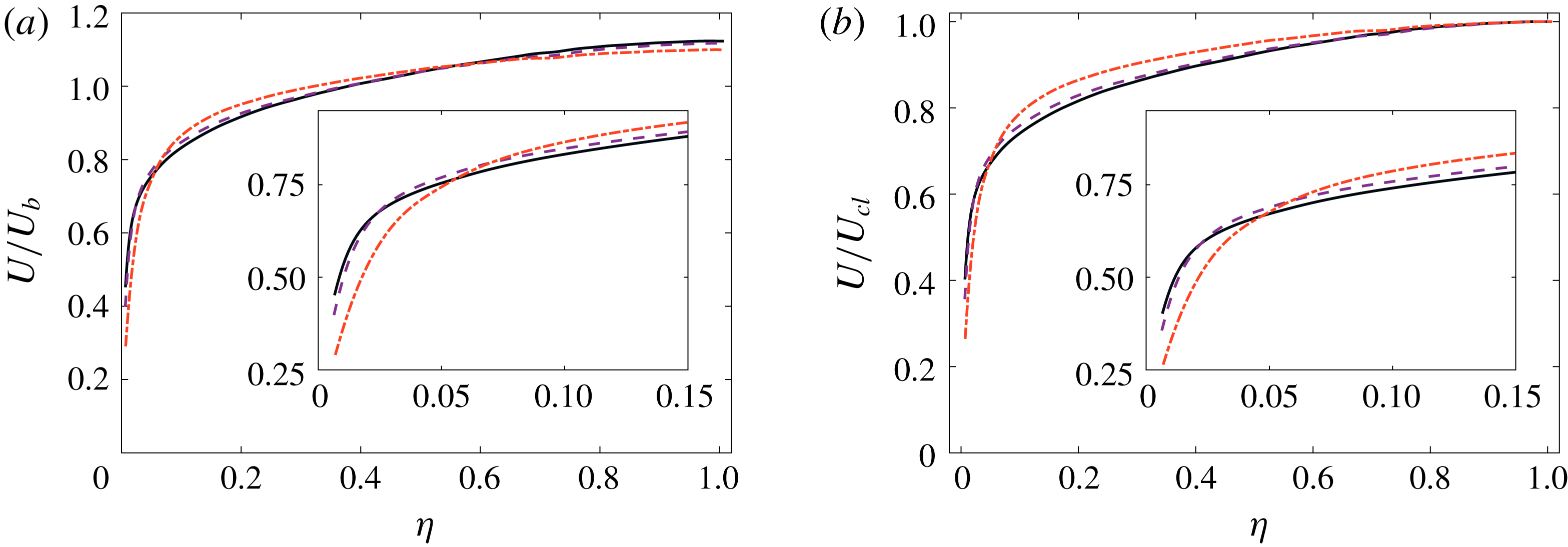
was held constant for increasing polymer concentration. Accordingly, redistributions of momentum or vorticity only result when there is a net modification, i.e. reduction, in drag. This behaviour is made clear in figure 9(a,b), which plots mean velocity profiles normalized by the bulk (spatially averaged) velocity,
 $U_{b}$
, and centreline velocity,
 $U_{cl}$
, respectively. Here, the near-wall velocity profile falls below the Newtonian flow, but for
 $\unicode[STIX]{x1D702}=y/\unicode[STIX]{x1D6FF}>0.05$
the profile exceeds the Newtonian case, and then falls below in a region near the centreline. The mass flow rate was held constant, and thus the conservation of mass requires an area-preserving profile. The redistribution of momentum away from the wall leads to a reduction in the velocity gradient near the wall. Consistently, the profiles at
 $\unicode[STIX]{x1D6FF}^{+}\approxeq 1800$
also exhibit the same qualitative behaviour as the lower-Reynolds-number case.
Mean velocity normalized with (a) the bulk velocity and (b) the centreline velocity. Solid line,
 $DR=0$
at
 $\unicode[STIX]{x1D6FF}^{+}\approxeq 1800$
; dash–dot line,
 $\unicode[STIX]{x1D6FF}^{+}=1463$
; dashed line,
 $\unicode[STIX]{x1D6FF}^{+}=1691$
.

A number of measures can be used to quantify aspects of the mean profile features just noted. One such integral measure is the displacement thickness,
 $\unicode[STIX]{x1D6FF}^{\ast }$
, as it reflects properties associated with mass conservation as well as those associated with the mean vorticity distribution. For the present planar channel, the equation for
 $\unicode[STIX]{x1D6FF}^{\ast }$
is given by
 $$\begin{eqnarray}\displaystyle \unicode[STIX]{x1D6FF}^{\ast }=\int _{0}^{\unicode[STIX]{x1D6FF}}\left(1-\frac{U}{U_{cl}}\right)\text{d}y. & & \displaystyle\end{eqnarray}$$
As first demonstrated mathematically by Lighthill (Reference Lighthill1958),
 $\unicode[STIX]{x1D6FF}^{\ast }$
has the precise physical interpretation as being the centroid of the mean vorticity distribution. This interpretation will be revisited in the discussion of (3.6) relative to the mean vorticity profile. The ratio of the displacement thickness in polymer flow,
 $\unicode[STIX]{x1D6FF}_{p}^{\ast }$
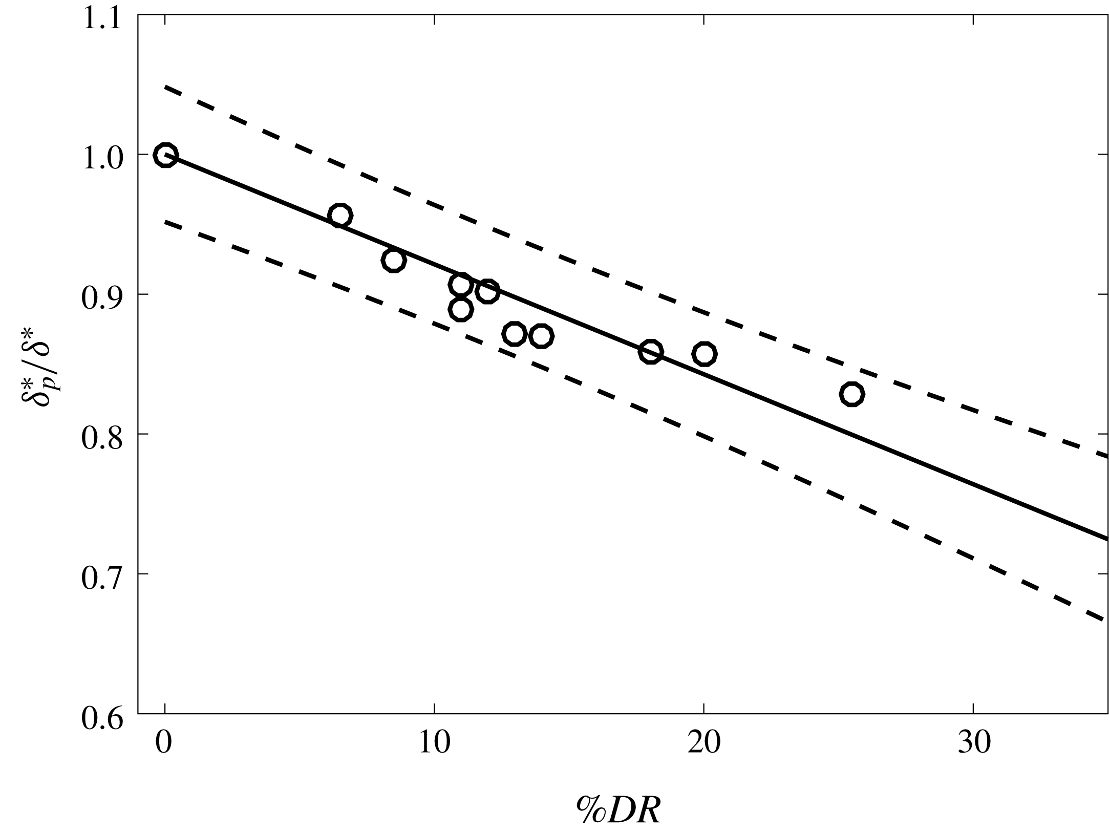
, to that in the experimental Newtonian flow,
 $\unicode[STIX]{x1D6FF}^{\ast }$
, is presented in figure 10. From this figure, it is apparent that the position of the mean vorticity centroid relative to that in Newtonian fluid flow decreases with increasing
 $DR$
. The curve fit of the data presented in figure 10 is given by
 $$\begin{eqnarray}\displaystyle \frac{\unicode[STIX]{x1D6FF}_{p}^{\ast }}{\unicode[STIX]{x1D6FF}^{\ast }}=-0.00786(\%DR)+1. & & \displaystyle\end{eqnarray}$$
Ratio of the measured displacement thickness in the polymer
 $DR$
flow to that in Newtonian fluid flow at a similar
 $\unicode[STIX]{x1D6FF}^{+}$
. The
 $\circ$
symbols are the experimental data, the solid line is the curve fit given by (3.4), and the dashed lines represent the bounds of the
 $95\,\%$
confidence interval.

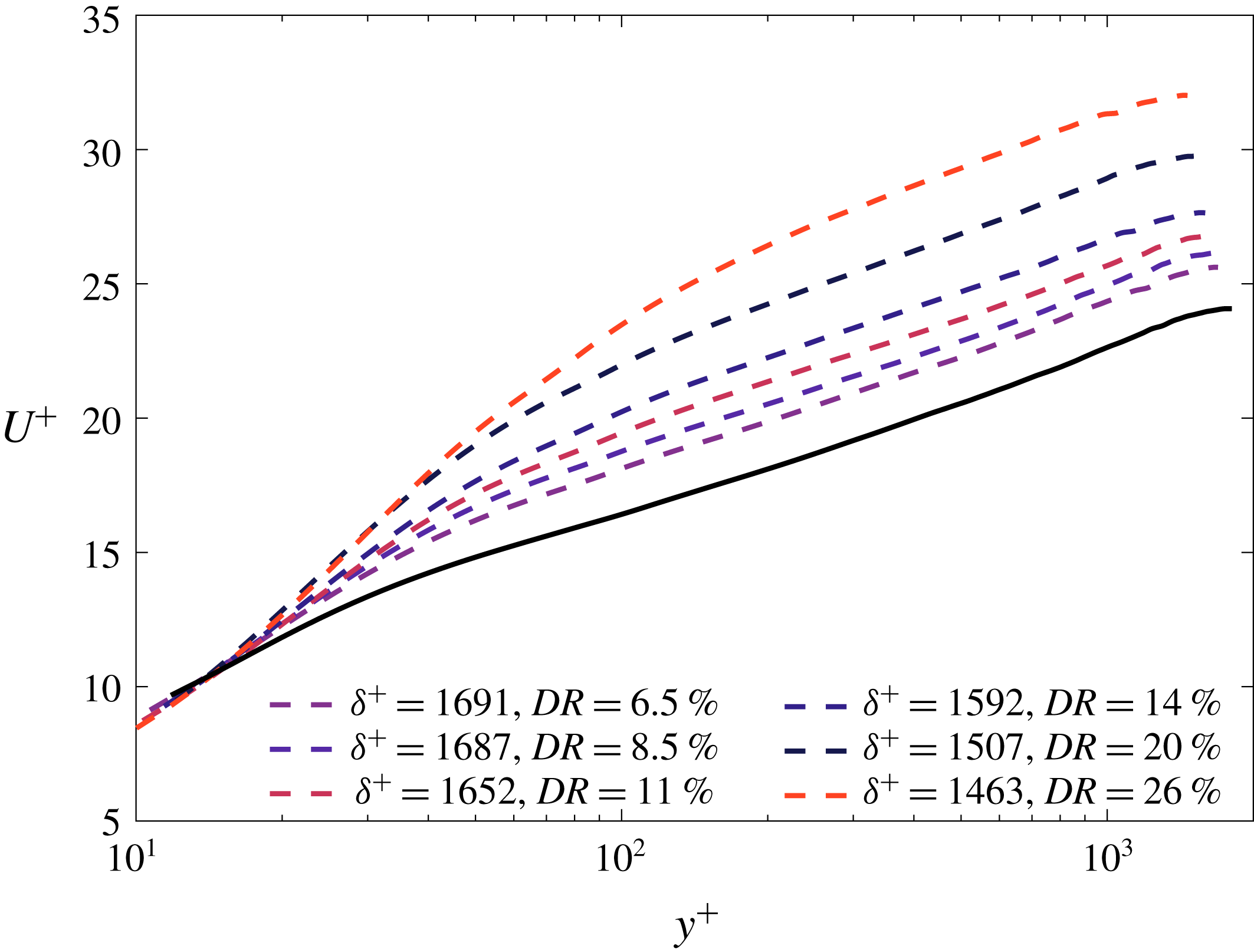
Inner-normalized mean velocity profiles. The solid line is for the
 $DR=0$
case at
 $\unicode[STIX]{x1D6FF}^{+}\approxeq 1800$
; dashed lines are for
 $DR>0$
.

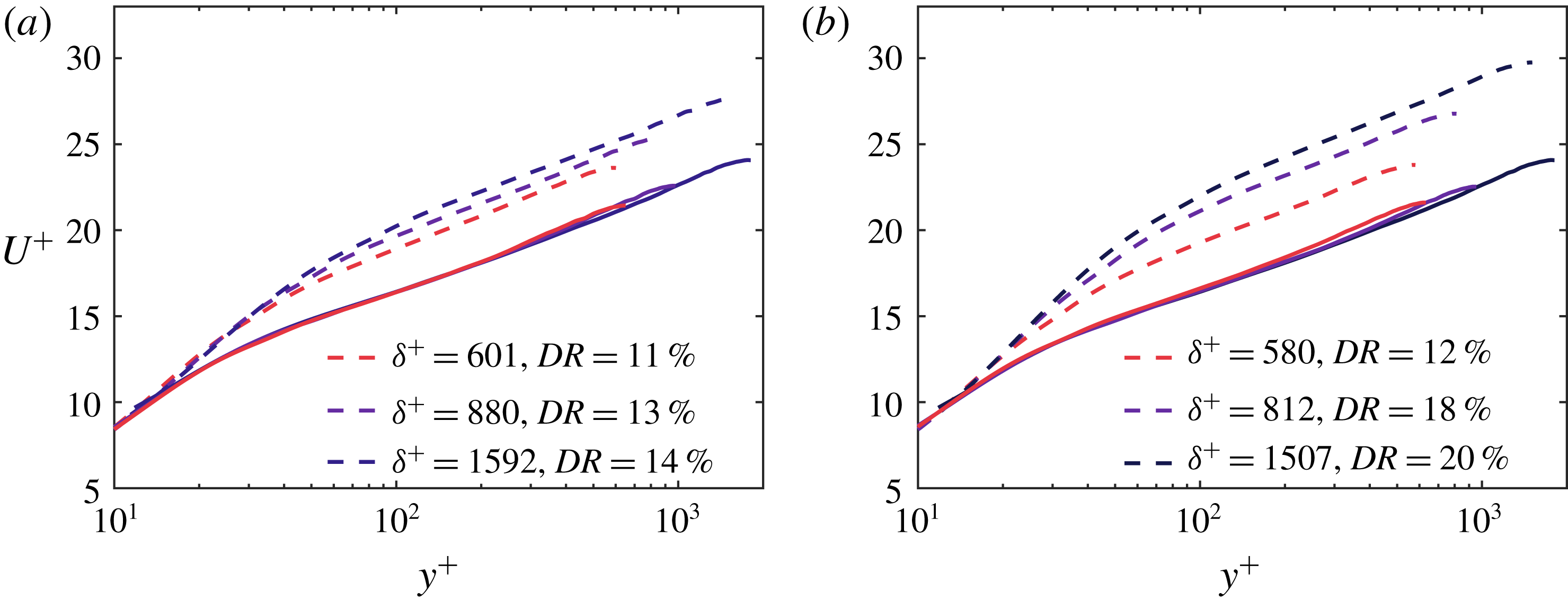
Inner-normalized velocity profiles for varying
 $\unicode[STIX]{x1D6FF}^{+}$
at two fixed injection concentrations: (a)
 $C_{i}=500$
wppm and (b)
 $C_{i}=1000~\text{wppm}$
. Solid lines correspond to
 $DR=0$
cases at
 $\unicode[STIX]{x1D6FF}^{+}\approxeq 650,975$
and
 $1800$
; dashed lines are for
 $DR>0$
cases.

3.4 Inner-normalized mean velocity profiles
Inner-normalized mean velocity profiles are presented in figures 11 and 12. The effect of injection concentration for a fixed initial
 $\unicode[STIX]{x1D6FF}^{+}$
is clearly presented in figure 11 whereas the effect of initial
 $\unicode[STIX]{x1D6FF}^{+}$
is clearly shown in figure 12. For pure water flow (
 $DR=0$
) Elsnab et al. (Reference Elsnab, Monty, White, Koochesfahani and Klewicki2017) showed that the 1c-MTV results exhibit excellent agreement with the similar
 $\unicode[STIX]{x1D6FF}^{+}$
DNS profiles. At a fixed initial
 $\unicode[STIX]{x1D6FF}^{+}$
, increasing the polymer concentration decreases the drag force. For
 $\unicode[STIX]{x1D6FF}^{+}\approxeq 650$
, however, increasing the concentration has minimal effect (see figure 12
a,b). This trend is also evident for the
 $\unicode[STIX]{x1D6FF}^{+}\approxeq 975$
case. These results indicate that, for injected polymers, the capacity of the polymer to reduce drag apparently depends on the concentration and the intensity of the turbulence, as nominally quantified by the magnitude of the Reynolds number. This intensity connects to the magnitude of the vorticity stretching and its associated capacity to stretch the polymer. It is well known that polymers do not reduce drag in laminar flow. The observations just noted would seem to be consistent with this phenomenon since vortex stretching is not present in laminar flows. More specifically, this observation also appears to be in accord with the results from the DNS simulations of Dubief et al. (Reference Dubief, White, Terrapon, Shaqfeh, Moin and Lele2004), indicating that large drag reductions correlate with the polymer chains undergoing a high degree of stretching.
The classical logarithmic equation for the mean velocity profile in statistically stationary turbulent wall-bounded flow is given by (1.1). The constant
 $\unicode[STIX]{x1D705}$
has special physical significance in this equation, as this leading coefficient reflects the slope of the profile, and thus is an average measure of how the turbulence distributes mean momentum as a function of
 $y$
(Klewicki, Fife & Wei Reference Klewicki, Fife and Wei2009). Accordingly, the mean flow theory based upon the leading balance structure of the mean momentum equation described in § 1.1 analytically connects
 $\unicode[STIX]{x1D705}$
to an asymptotically constant flux of turbulent inertial force (Klewicki et al.
Reference Klewicki, Philip, Marusic, Chauhan and Morrill-Winter2014). More generally, since
 $\unicode[STIX]{x1D705}$
is a manifestation of the underlying dynamical behaviours of wall-bounded flow, understanding how polymers modify
 $\unicode[STIX]{x1D705}$
is important to understanding the dynamics of polymer drag-reduced flow and, consequently, the overall phenomena of polymer drag reduction (White et al.
Reference White, Dubief and Klewicki2012, Reference White, Dubief and Klewicki2018).
Empirical estimation of the value of
 $\unicode[STIX]{x1D705}$
requires specification of the relevant flow domain. Herein, the slope of the logarithmic mean profile is determined by curve-fitting the inner-normalized velocity profiles. In accord with the leading balance structure of (1.3), the domain of this fit is beyond the peak in the combined Reynolds and polymer stress,
 $1.5y_{m}$
, to
 $y=0.2\unicode[STIX]{x1D6FF}$
. As revealed later in figures 19 and 20, this is where the profiles of the
 $RPS$
are essentially parallel to the corresponding
 $DR=0$
profile. Relative to the leading balance structure of figure 1, this corresponds to a position slightly beyond the start of layer
 $IV$
and extending into the lower portion of layer
 $IV$
(Klewicki et al.
Reference Klewicki, Fife, Wei and McMurtry2007). Physically, the start of this domain is where the viscous force loses leading order. Consistent with the notion of an inertial sublayer in physical space, the end of the specified domain extends to only a small fraction of
 $\unicode[STIX]{x1D6FF}$
, and is well within the theoretically estimated bounds of the domain where (1.2) admits a self-similar invariant form owing to a constant wallward flux of turbulent inertial force (Klewicki Reference Klewicki2013b
). The specified domain of the logarithmic profile is consistent with the high-Reynolds-number data analysis of Marusic et al. (Reference Marusic, Monty, Hultmark and Smits2013), and has also been shown to reliably locate the inertial sublayer in rough-wall flows (Mehdi, Klewicki & White Reference Mehdi, Klewicki and White2013; Ebner, Mehdi & Klewicki Reference Ebner, Mehdi and Klewicki2016; Squire et al.
Reference Squire, Morrill-Winter, Hutchins, Schultz, Klewicki and Marusic2016).
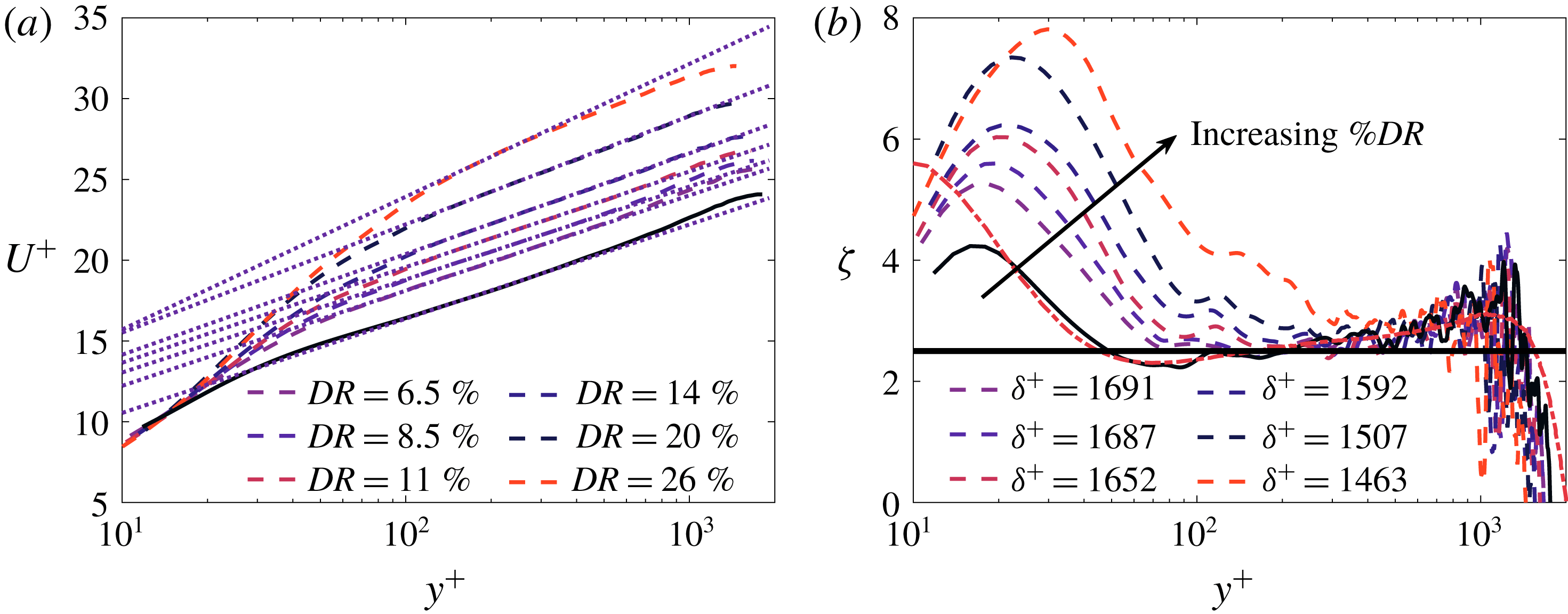
Examination of figure 13(a) suggests that the estimated value of
 $\unicode[STIX]{x1D705}$
begins changing for
 $DR$
values much less than the
 $40\,\%$
threshold found by Warholic et al. (Reference Warholic, Massah and Hanratty1999). Conversely, these results reinforce the observation of White et al. (Reference White, Dubief and Klewicki2012) that polymer effects do not adhere to the Virk model (Virk Reference Virk1975).
The indicator function (
 $\unicode[STIX]{x1D701}=y^{+}\text{d}U/\text{d}y^{+}$
) is commonly used to empirically assess the existence of logarithmic profile variation. The
 $\unicode[STIX]{x1D701}$
estimates from the present data are given in figure 13(b). These data show a region of local minima approaching a constant,
 $1/\unicode[STIX]{x1D705}$
, indicating logarithmic dependence. Although the mean velocity distribution in the buffer layer appears logarithmic in wall coordinates, the indicator function reveals that it is clearly not logarithmic. This test further indicates that for non-zero
 $DR$
,
 $\unicode[STIX]{x1D705}$
exhibits convincing deviations from the Newtonian flow value, and that there is no dip in
 $\unicode[STIX]{x1D701}$
below
 $1/\unicode[STIX]{x1D705}$
for
 $DR\gtrsim 10\,\%$
. This second feature is due to the manner by which
 $\text{d}U^{+}/\text{d}y^{+}$
decays with distance from the wall, as exemplified by where the profiles in figure 15 take on their outer region approach towards zero. Note that with increasing
 $DR$
this occurs increasingly farther from the wall than in the Newtonian case. Consistently, the log-layer (as defined) is also farther from the wall, and at
 $DR=26\,\%$
there is scant evidence of an inertially dominated region. Similar behaviours have also been observed in the HDR regime (
 $DR>40\,\%$
) (Warholic et al.
Reference Warholic, Massah and Hanratty1999; White et al.
Reference White, Dubief and Klewicki2018), but, to the authors’ knowledge, have not been previously reported relative to the LDR values studied herein. Overall, the present mean profile behaviours support the description given in White et al. (Reference White, Dubief and Klewicki2018).
Curve fits for the mean velocity used to estimate
 $\unicode[STIX]{x1D705}$
(a) and the associated indicator function
 $\unicode[STIX]{x1D701}$
(b). Solid line,
 $DR=0$
at
 $\unicode[STIX]{x1D6FF}^{+}\approxeq 1800$
; dashed lines are
 $DR>0$
; dotted lines are the curve fits over
 $1.5y_{m}\lesssim y\lesssim 0.2\unicode[STIX]{x1D6FF}$
; the thick line denotes the slope of
 $1/\unicode[STIX]{x1D705}=1/0.4$
.

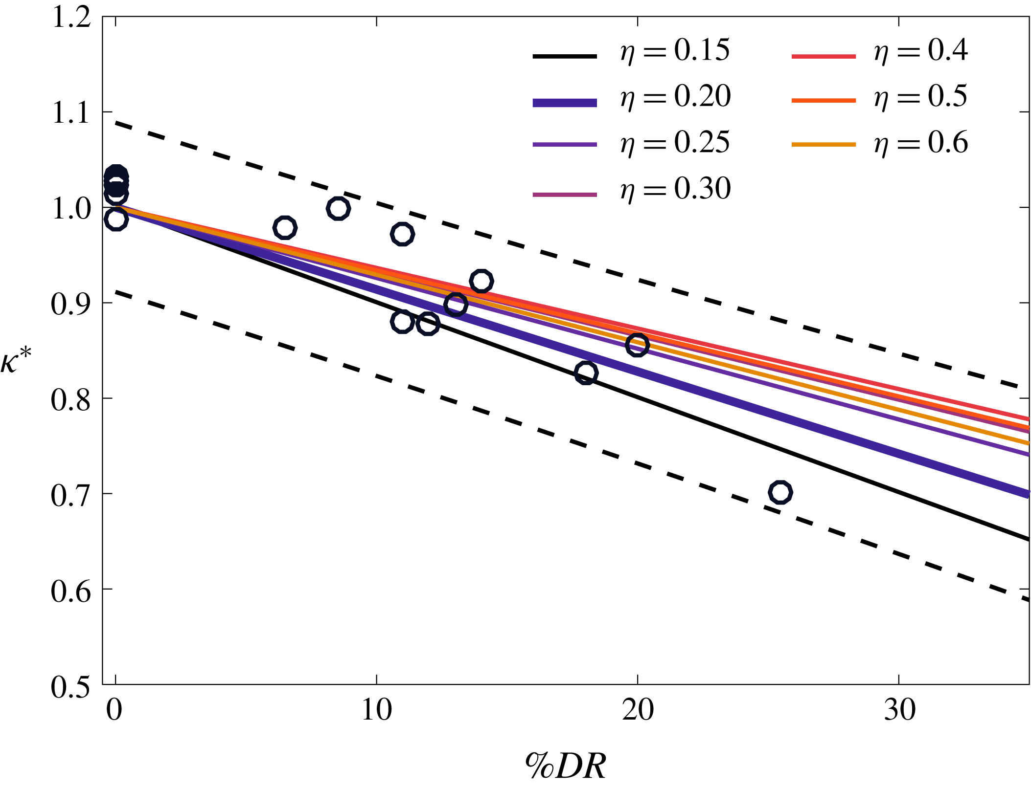
Normalized slope of the log region, where
 $\unicode[STIX]{x1D705}^{\ast }=\unicode[STIX]{x1D705}_{p}/\unicode[STIX]{x1D705}$
and
 $\unicode[STIX]{x1D705}=0.4$
. The
 $\circ$
symbols are the experimental data for
 $\unicode[STIX]{x1D702}=0.2$
; solid lines are linear curve fits for
 $\unicode[STIX]{x1D702}=0.15,0.2,0.25,0.3,0.4,0.5,0.6$
and
 $1.5y_{m}^{+}$
; the dashed lines denote the
 $95\,\%$
confidence interval for
 $\unicode[STIX]{x1D702}=0.2$
.

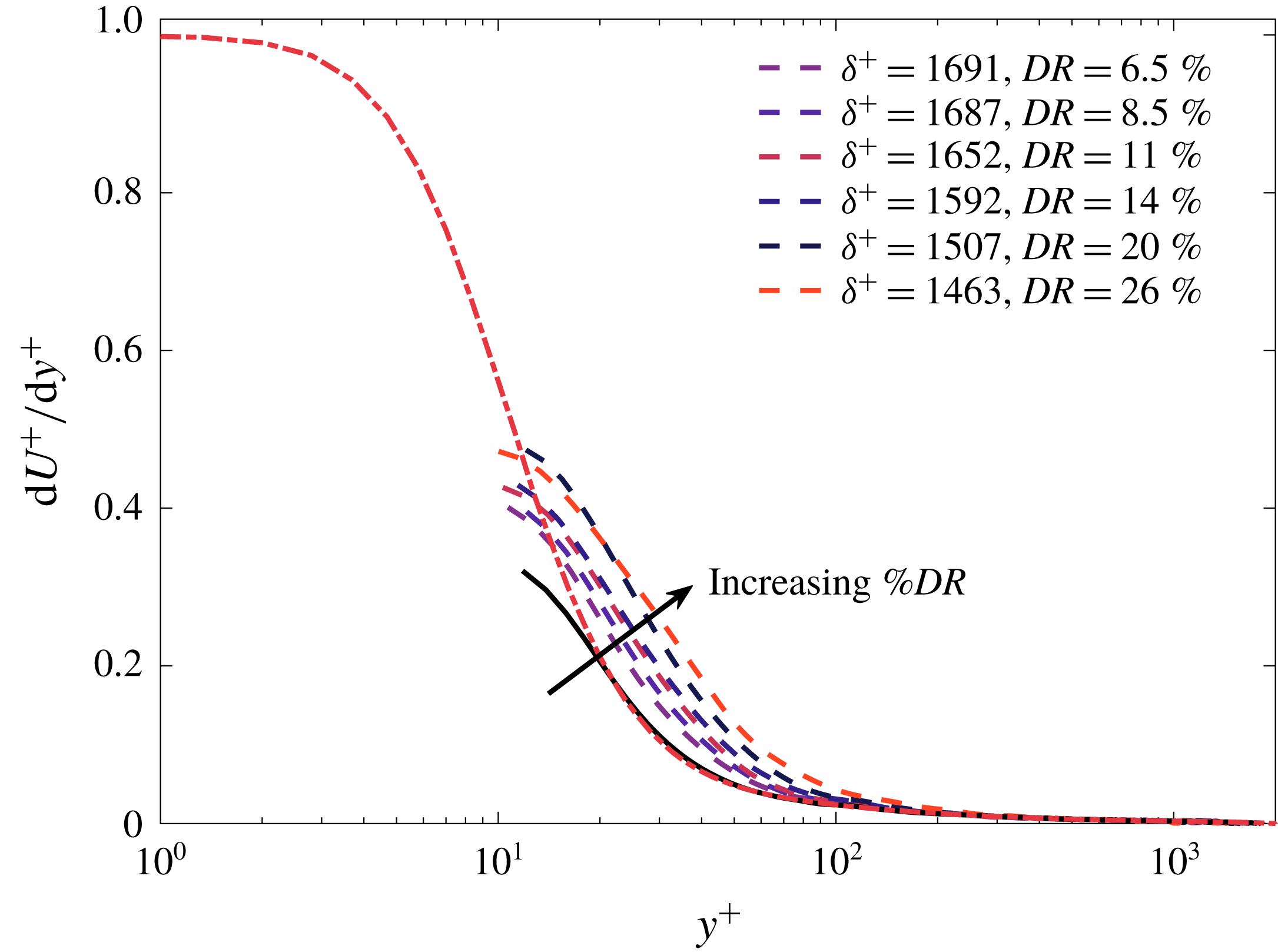
Mean velocity gradient profiles. Solid line,
 $DR=0$
at
 $\unicode[STIX]{x1D6FF}^{+}\approxeq 1800$
; dashed lines denote
 $DR>0$
cases; dash–dot line, DNS at
 $\unicode[STIX]{x1D6FF}^{+}=2004$
.

Indeed, in the direct comparisons now described, the data indicate continuous variations in
 $\unicode[STIX]{x1D705}$
that are in excess of the
 $95\,\%$
uncertainty bound for
 $DR$
values greater than approximately
 $15\,\%$
. Furthermore, based upon the data trend, this variation would seem to begin for
 $DR\lesssim 15\,\%$
. The relevant results are depicted in figure 14, where the end point of the logarithmic region used to determine
 $\unicode[STIX]{x1D705}$
via a linear curve fit is varied from
 $\unicode[STIX]{x1D702}=0.15,0.2,0.25,0.3,0.4,0.5,0.6$
(see figure 13(a) for an example of the curve fit). The start point for the curve fit is
 $1.5\times$
the peak location in the combined Reynolds and polymer stress. This moves the start point to within layer
 $IV$
(i.e. well within the inertial layer) and ensures that the curve-fit region is not biased by the transition regime. A conservative minimum end point of
 $\unicode[STIX]{x1D702}=0.15$
was used by Marusic et al. (Reference Marusic, Monty, Hultmark and Smits2013), while Pope (Reference Pope2000) reported
 $\unicode[STIX]{x1D702}=0.3$
. These two values are the lower and upper bounds reported in the literature for the end point of the logarithmic region. Note that using values of
 $\unicode[STIX]{x1D702}>0.3$
violates the notion that the log-layer is an inertial sublayer, so the results presented in figure 14 for
 $\unicode[STIX]{x1D702}>0.3$
should be interpreted with caution, as the end point is likely beyond the logarithmic region. Here it is shown that the slope of the log-layer profile normalized by the Newtonian value (
 $\unicode[STIX]{x1D705}=0.4$
) decreases approximately linearly with increasing
 $DR$
. It is clear that there is an effect on the slope that is dependent upon the end point of the log-layer, but all of the fits lie within the
 $95\,\%$
confidence interval for an end point of
 $\unicode[STIX]{x1D702}=0.2$
and start point of
 $1.5y_{m}^{+}$
. As just noted, it is also evident that a change in slope is nearly a statistical surety for
 $DR\gtrsim 15\,\%$
, and that these changes are much larger than those one might attribute to variations in Reynolds number. A curve fit of the data in figure 13 for
 $\unicode[STIX]{x1D702}=0.2$
is given by
 $$\begin{eqnarray}\displaystyle \unicode[STIX]{x1D705}^{\ast }=\frac{\unicode[STIX]{x1D705}_{p}}{\unicode[STIX]{x1D705}}=-0.0086(\%DR)+1. & & \displaystyle\end{eqnarray}$$
Note that under the condition of
 $DR=0$
, one would expect the data to reflect the Newtonian flow value, and thus an additive coefficient of
 $1.0$
. This condition is enforced for (3.5). If a floating parameter fit is performed, the data fit is within approximately
 $3\,\%$
of this value.
3.5 Mean velocity gradient
The mean velocity gradient (
 $\text{d}U^{+}/\text{d}y^{+}$
) was estimated using a second-order forward finite difference scheme. As is apparent, the
 $DR=0$
profile of figure 15 exhibits very good agreement with the DNS data for
 $y^{+}\gtrsim 20$
. As expected, the profiles for
 $DR>0$
indicate a redistribution of mean vorticity,
 $\text{d}U^{+}/\text{d}y^{+}=-\unicode[STIX]{x1D6FA}_{z}$
. Here it is relevant to note that the displacement thickness is equivalently given by
 $$\begin{eqnarray}\displaystyle \unicode[STIX]{x1D6FF}^{\ast }=\frac{\displaystyle \int _{0}^{\unicode[STIX]{x1D6FF}}y\unicode[STIX]{x1D6FA}_{z}\,\text{d}y}{\displaystyle \int _{0}^{\unicode[STIX]{x1D6FF}}\unicode[STIX]{x1D6FA}_{z}\,\text{d}y}, & & \displaystyle\end{eqnarray}$$
indicating that
 $\unicode[STIX]{x1D6FF}^{\ast }$
is the centroid of the mean vorticity distribution. The trend in the profiles of figure 15 is seen to be consistent with the data of figure 10 by recognizing that the integrand contributions to (3.3) over a range of relatively large
 $y$
, or equivalently, the large
 $y$
contributions to the numerator in (3.6), are reduced under the influence of the polymer. (Also see the changes to the mean profile shape in figure 9.)
3.6 Streamwise velocity RMS profiles
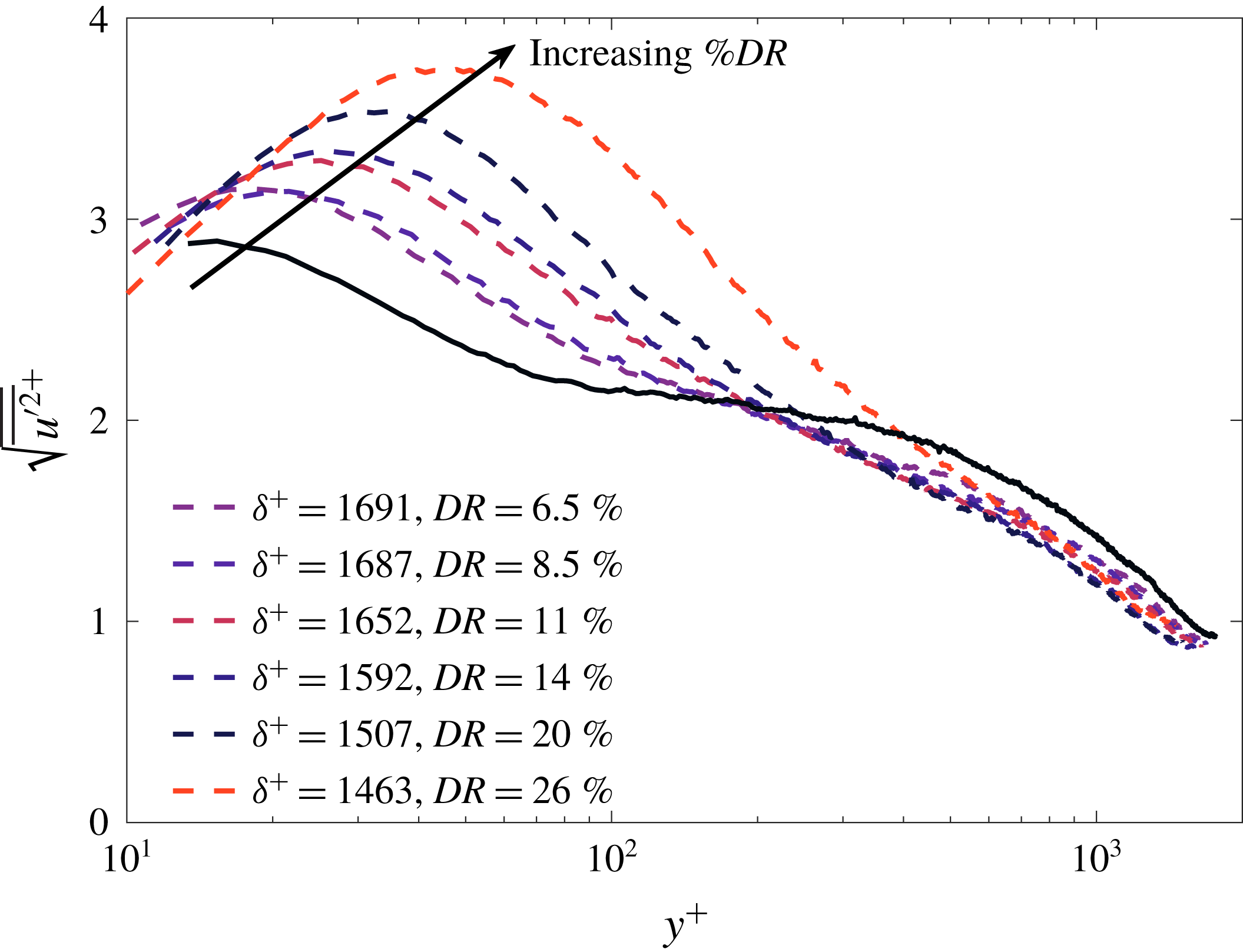
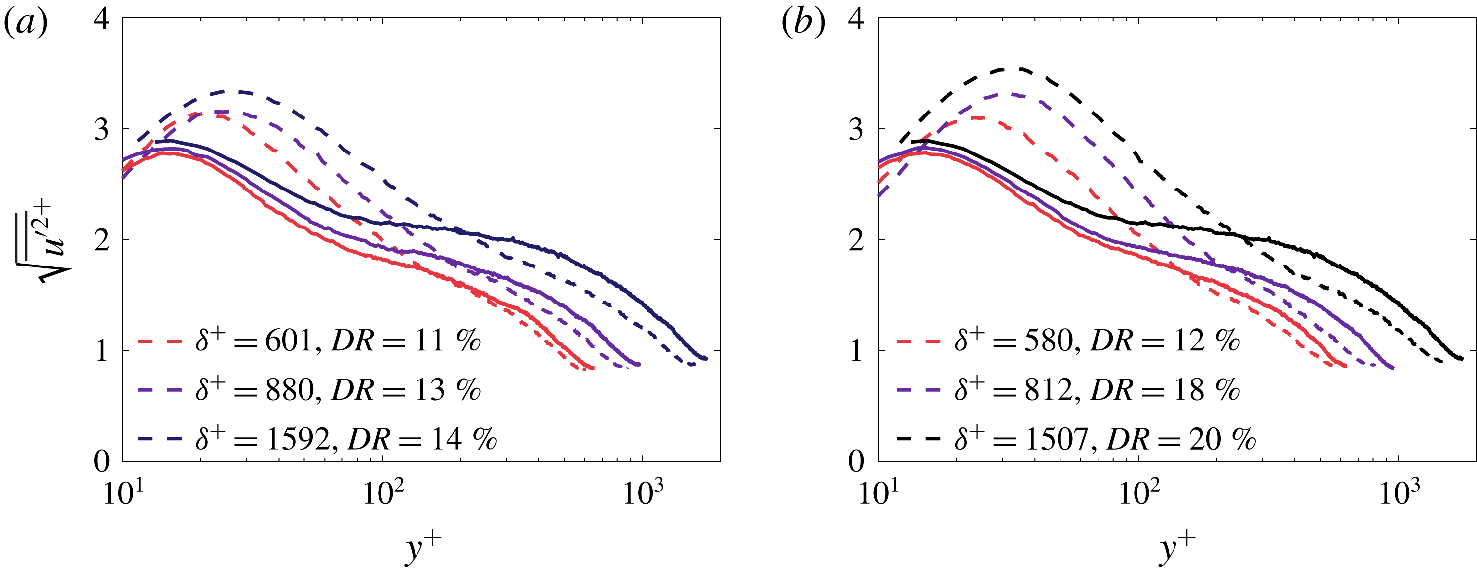
The present inner-normalized streamwise velocity r.m.s. profiles are shown in figures 16 and 17. With increasing
 $DR$
, the peak r.m.s.
 $u^{\prime }$
values increase, as does the
 $y^{+}$
position,
 $y_{p}^{+}$
, of this peak. Consistent with the previous results of Warholic et al. (Reference Warholic, Massah and Hanratty1999), this trend reinforces their physical interpretation that increasing the Reynolds number increases the capacity of the polymer at a fixed injection flow rate/concentration to reduce skin friction. This trend is illustrated in figure 17. Here it is noted that an increase in
 $\sqrt{\overline{u^{\prime 2+}}}$
is primarily attributable to a decrease in
 $u_{\unicode[STIX]{x1D70F}}$
, with
 $\sqrt{\overline{u^{\prime 2}}}$
remaining nearly constant (White & Mungal Reference White and Mungal2008). Thus, the reduction in skin friction could either be associated with a decrease in the intensity of
 $\sqrt{\overline{v^{\prime 2+}}}$
, or by an off-setting decrease in the correlating interaction between
 $u^{\prime }$
and
 $v^{\prime }$
. A decrease in
 $v^{\prime }$
is consistent with the existing literature (Wei & Willmarth Reference Wei and Willmarth1992; Warholic et al.
Reference Warholic, Massah and Hanratty1999), and with the notion that polymers modify the momentum mixing (homogenization) mechanisms associated with the near-wall vorticity field (White et al.
Reference White, Dubief and Klewicki2018). The physics of the associated energetics are discussed extensively by Dubief et al. (Reference Dubief, White, Terrapon, Shaqfeh, Moin and Lele2004). Their physical premise is that the polymer extracts energy from the buffer-layer vortices and releases it in the near-wall streaks, leading to enhanced
 $u^{\prime }$
and reduced
 $v^{\prime }$
.
Streamwise velocity r.m.s. profiles. The solid line denotes the
 $DR=0$
case at
 $\unicode[STIX]{x1D6FF}^{+}\approxeq 1800$
; dashed lines denote
 $DR>0$
cases.

Streamwise velocity r.m.s. profiles for (a)
 $C_{i}=500$
wppm and (b)
 $C_{i}=1000$
wppm. Solid line,
 $DR=0$
at
 $\unicode[STIX]{x1D6FF}^{+}\approxeq 650,975,1800$
; dashed lines denote
 $DR>0$
cases.

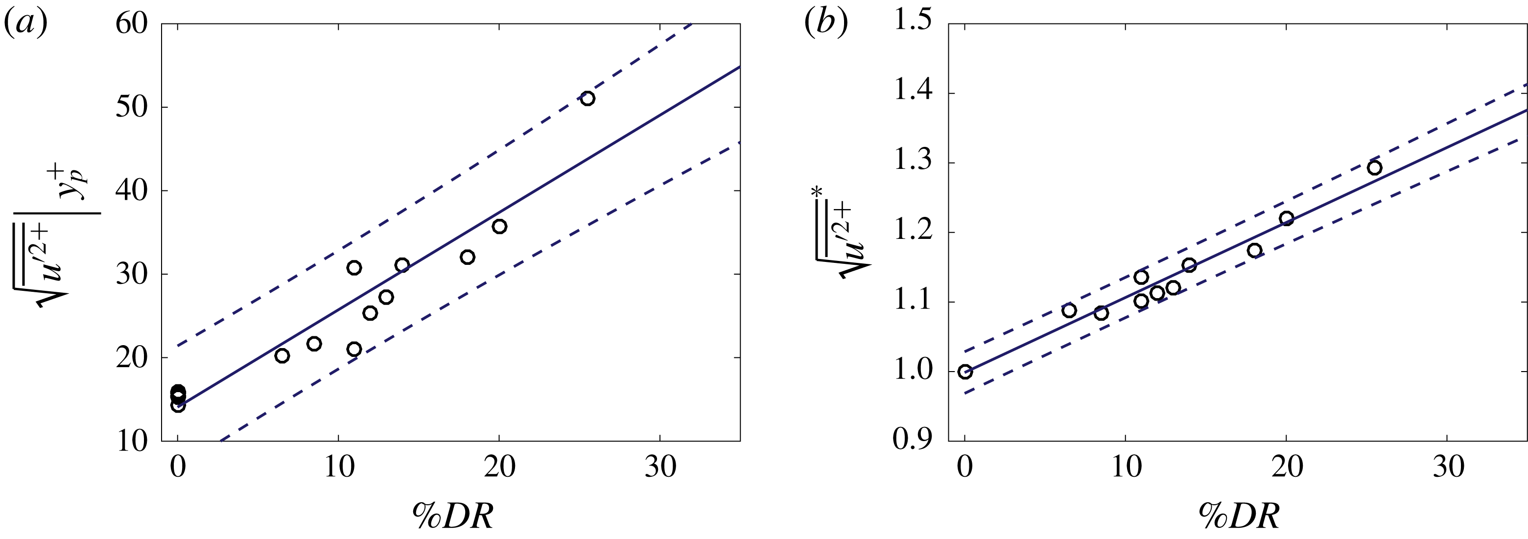
The present data allow the rate at which
 $y_{p}^{+}$
increases to be quantified as a function of
 $DR$
. The position of these peaks is plotted in figure 18(a). According to these data, the outward movement of the peak is nearly linear with
 $DR$
, as exemplified by the curve fit
 $$\begin{eqnarray}\displaystyle \sqrt{\overline{u^{\prime 2+}}}|_{y_{p}^{+}}=1.165(\%DR)+14.1. & & \displaystyle\end{eqnarray}$$
In figure 18(b), the polymer flow peak r.m.s.
 $u^{\prime }$
data are normalized by the peak value in the Newtonian flow, with the normalization denoted by an asterisk. A curve fit of the data yields
 $$\begin{eqnarray}\displaystyle \sqrt{\overline{u^{\prime 2+}}}^{\ast }=0.011(\%DR)+1.0. & & \displaystyle\end{eqnarray}$$
To the authors’ knowledge the quantifications of figure 18 are the clearest elucidation of these trends to date.


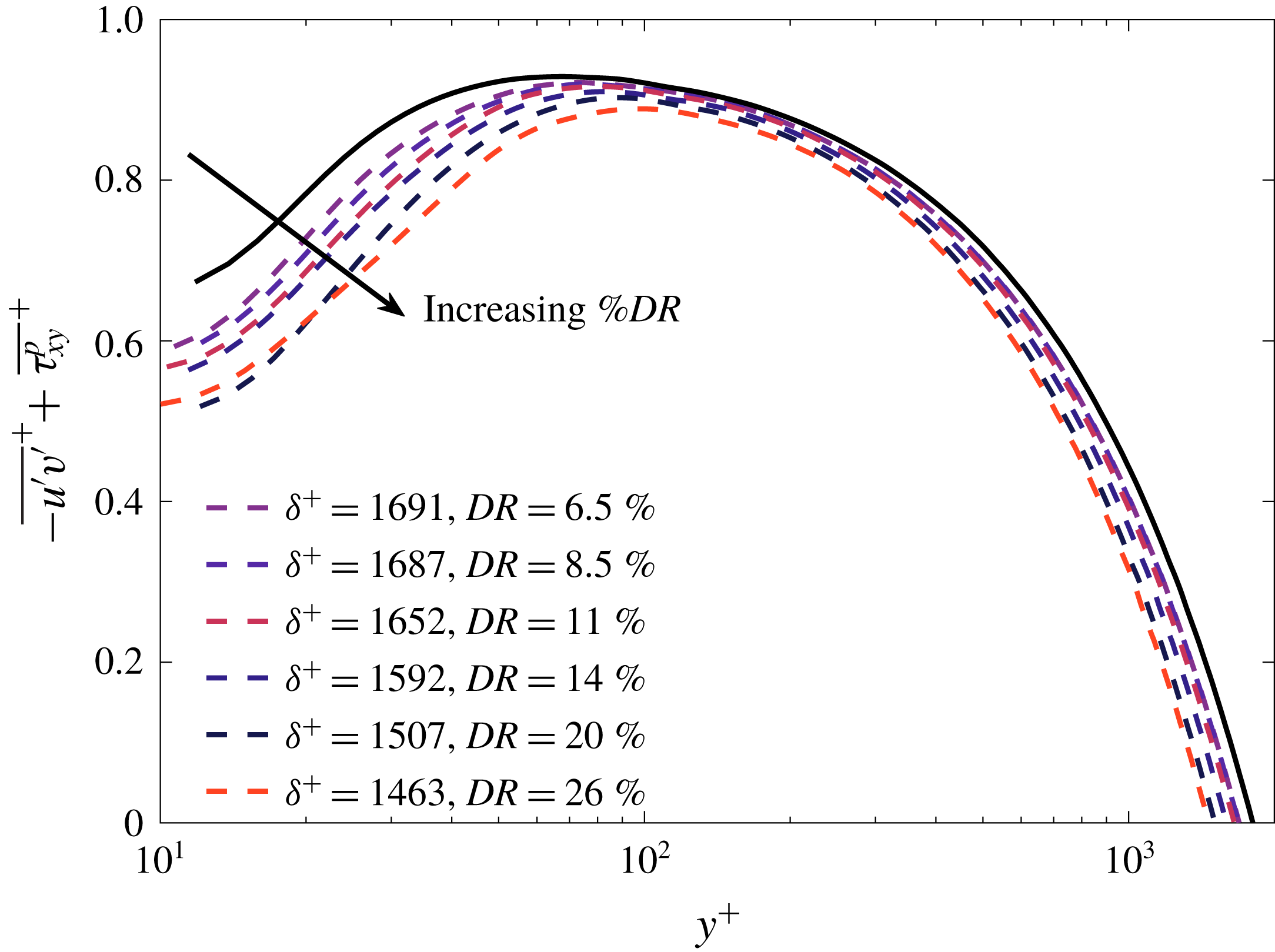
3.7 Combined Reynolds and polymer stress profiles
Reynolds and polymer stress
 $(RPS)$
profiles were obtained from the measured mean velocity gradient profiles, and the integrated mean momentum equations (1.4) and (1.5), respectively. These stress profiles are presented in figure 19. Under the influence of polymer, the inner-normalized peak in the combined stress decreases and moves outwards in viscous units with increasing
 $DRu^{\prime 2+}$
. This is consistent with the previous observation indicating that while
 $\sqrt{\overline{u^{\prime 2+}}}$
increases,
 $\sqrt{\overline{v^{\prime 2+}}}$
decreases (Warholic et al.
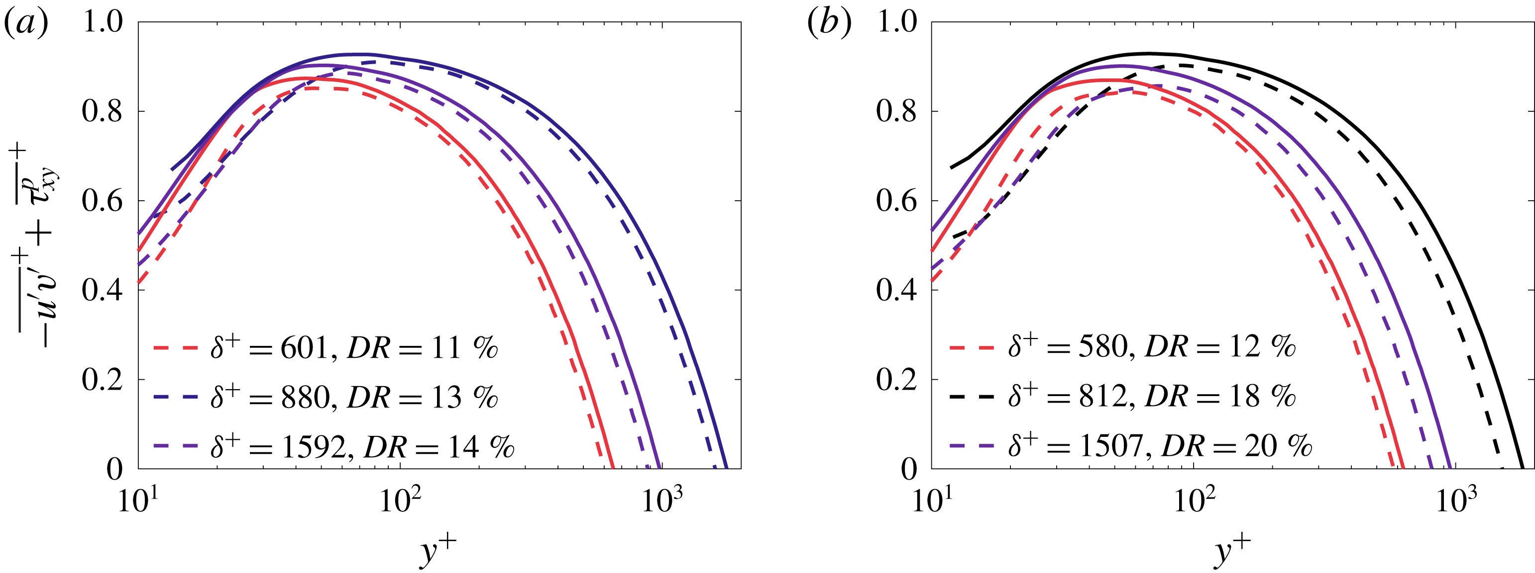
Reference Warholic, Massah and Hanratty1999). Here it is useful to reiterate, however, that the polymer stress cannot be independently determined from the present experiments. After close inspection, it is also apparent from figure 20 that the capacity of the injected polymer to reduce skin friction is Reynolds number dependent. This is exemplified by the
 $RPS$
profile at
 $\unicode[STIX]{x1D6FF}^{+}\simeq 650$
, which shows minimal change even though the injected polymer concentration doubled. Upon increasing
 $\unicode[STIX]{x1D6FF}^{+}$
to
 $975$
, however, the
 $RPS$
shows an increasing deviation with increasing concentration. It is also clear from figure 20 that the modification of the combined stress profiles occurs in the near-wall region with a much smaller (essentially immeasurable) effect on the outer region when compared to the Newtonian flows at similar
 $\unicode[STIX]{x1D6FF}^{+}$
. This behaviour is consistent with the polymer modifying the vorticity stretching and reorientation processes that underlie the three-dimensionalization of the near-wall vorticity field (for example, White et al.
Reference White, Dubief and Klewicki2018).
Reynolds plus polymer stress profiles. Solid line,
 $DR=0$
at
 $\unicode[STIX]{x1D6FF}^{+}\approxeq 1800$
; dashed lines denote
 $DR>0$
cases.

Reynolds and polymer stress for two fixed injection concentrations, (a)
 $C_{i}=500$
wppm, and (b)
 $C_{i}=1000$
wppm. Solid line,
 $DR=0$
at
 $\unicode[STIX]{x1D6FF}^{+}\approxeq 650,975,$
and
 $1800$
; dashed lines denote
 $DR>0$
cases.

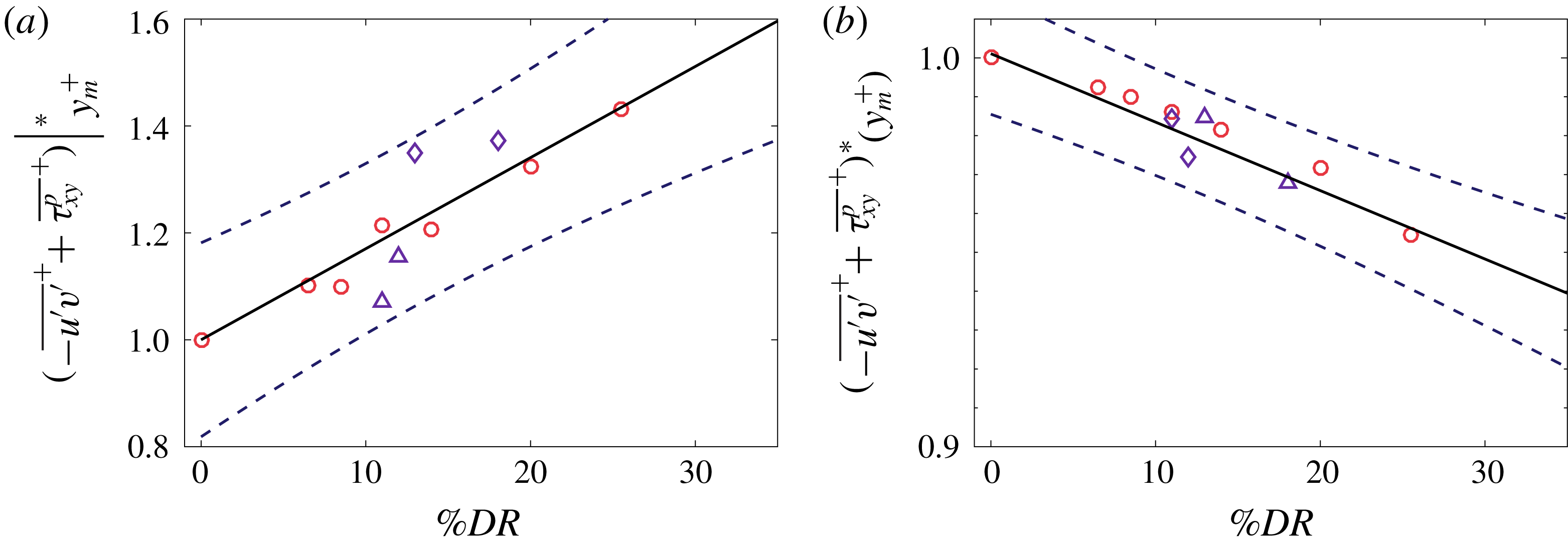
Normalized maximum position (a) and value (b) of the
 $RPS$
versus
 $DR$
. Newtonian baseline
 $\unicode[STIX]{x1D6FF}^{+}$
,
 $\circ \,\approxeq \,\unicode[STIX]{x1D6FF}_{1800}^{+}$
,
 $\diamond \,\approxeq \,\unicode[STIX]{x1D6FF}_{975}^{+}$
,
 $\triangle \,\approxeq \,\unicode[STIX]{x1D6FF}_{650}^{+}$
; solid line, curve fit; dashed line,
 $95\,\%$
confidence interval.

The
 $y^{+}$
location of the maximum
 $RPS$
value, as normalized by its experimental Newtonian value, moves outwards approximately linearly with
 $DR$
, as shown in figure 21(a). The curve fit on this figure is given by
 $$\begin{eqnarray}\displaystyle RPS^{+}|_{y_{m}^{+}}^{\ast }=(-\overline{u^{\prime }v^{\prime }}^{+}+\overline{\unicode[STIX]{x1D70F}_{xy}^{p}}^{+})|_{y_{m}^{+}}^{\ast }=0.0174(\%DR)+1. & & \displaystyle\end{eqnarray}$$
Similarly, the normalized maximum value decays approximately linearly, as shown in figure 21(b), and decays according to
 $$\begin{eqnarray}\displaystyle RPS^{+\ast }(y^{+}=y_{m}^{+})=-0.00176(\%DR)+1. & & \displaystyle\end{eqnarray}$$
The trend of figure 21(a) directly correlates with the outward movement (in
 $y^{+}$
) of the inertial domain with increasing
 $DR$
. This is because the peak in the
 $RPS$
coincides with an exchange in leading-order balance that culminates with the
 $VF$
term becoming subdominant. This and other effects on the structure of the mean dynamical balance are now investigated in greater detail.
3.8 Analyses based on the MMB
The above data presentation largely employed the traditional means by which to represent and interpret the statistical profiles of wall turbulence. As demonstrated by comparing smooth- and rough-wall flows (Mehdi et al.
Reference Mehdi, Klewicki and White2013; Ebner et al.
Reference Ebner, Mehdi and Klewicki2016; Squire et al.
Reference Squire, Morrill-Winter, Hutchins, Schultz, Klewicki and Marusic2016), and most recently for polymer flow (White et al.
Reference White, Dubief and Klewicki2018), data representations and interpretations in the context of the MMB provide new insights into the underlying dynamics. Accordingly, the present section first reveals and characterizes the modifications to the four-layer structure of the MMB under the influence of polymer, and then self-consistently uses this structure to revisit the behaviours of some of the statistical profiles just examined. In the following sections, data presentation focuses on the higher-
 $\unicode[STIX]{x1D6FF}^{+}$
data set. These data exhibit clear trends in the MMB structure.
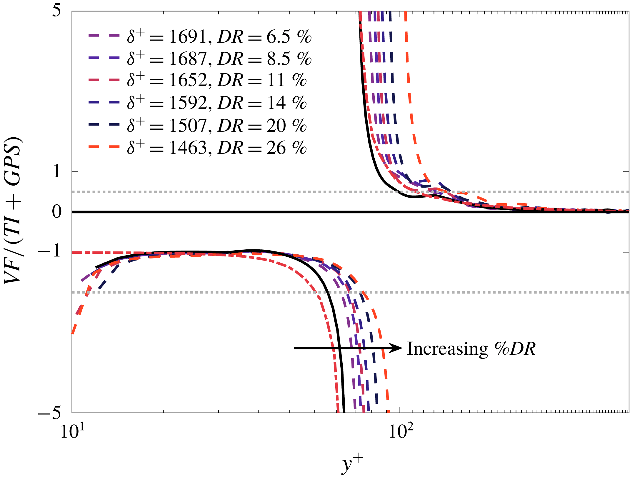
The experimental version of figure 1 is presented in figure 22. Per (1.3), generating the profiles in figure 22 requires taking the ratio of two quantities that depend on the second
 $y$
derivative of the experimentally determined mean velocity profile. Assessment of the veracity of these profiles is reflected in the very good agreement between the measured ratio profiles for Newtonian flow, as compared to the DNS profiles at similar Reynolds number.
Profiles of
 $VF/(TI+GPS)$
. Solid line,
 $DR=0$
at
 $\unicode[STIX]{x1D6FF}^{+}\approxeq 1800$
; dashed lines denote
 $DR>0$
cases; dash–dot line, DNS at
 $\unicode[STIX]{x1D6FF}^{+}=2004$
.

For Newtonian flows, a subjectively yet self-consistently defined end point criterion for layer
 $II$
was incorporated in the analysis of Wei et al. (Reference Wei, Fife, Klewicki and McMurtry2005). Namely, this is where the ratio of
 $VF/TI=-2$
. Similarly, the end of layer
 $III$
is where
 $VF/TI=0.5$
. Using these criteria, the effect of the polymer on the layer bounds can be determined by finding where
 $VF/(TI+GPS)=-2$
and
 $0.5$
. For Newtonian flows, the
 $y^{+}$
end points of layers
 $II$
and
 $III$
are respectively well represented by
 $1.6\sqrt{(\unicode[STIX]{x1D6FF}^{+})}$
and
 $2.6\sqrt{(\unicode[STIX]{x1D6FF}^{+})}$
(Wei et al.
Reference Wei, Fife, Klewicki and McMurtry2005; Klewicki Reference Klewicki2013b
). A curve fit of the present Newtonian data for layer
 $II$
yields
 $1.53(\unicode[STIX]{x1D6FF}^{+})^{0.49}$
and for layer
 $III$
yields
 $5.9(\unicode[STIX]{x1D6FF}^{+})^{0.38}$
. The deviation in the experimental result for layer
 $III$
is likely influenced by the uncertainty in our ability to precisely find where the profiles cross
 $0.5$
. For polymer-influenced flows, it is clear that the mean viscous force retains leading order farther from the wall, and accordingly the end point of layer
 $II$
moves to greater
 $y^{+}$
. Consistently, it is similarly apparent from figure 22 that the width and end point of layer
 $III$
also increases. Further evidence that the width of layer
 $III$
increases is given by (3.11) and (3.12). This is also due to the viscous force retaining significance to greater distances from the wall.
Equations (3.11) and (3.12) are curve-fit functions of
 $\unicode[STIX]{x1D6FF}^{+}$
and
 $DR$
. These describe additive corrections to the end points of layers
 $II$
and
 $III$
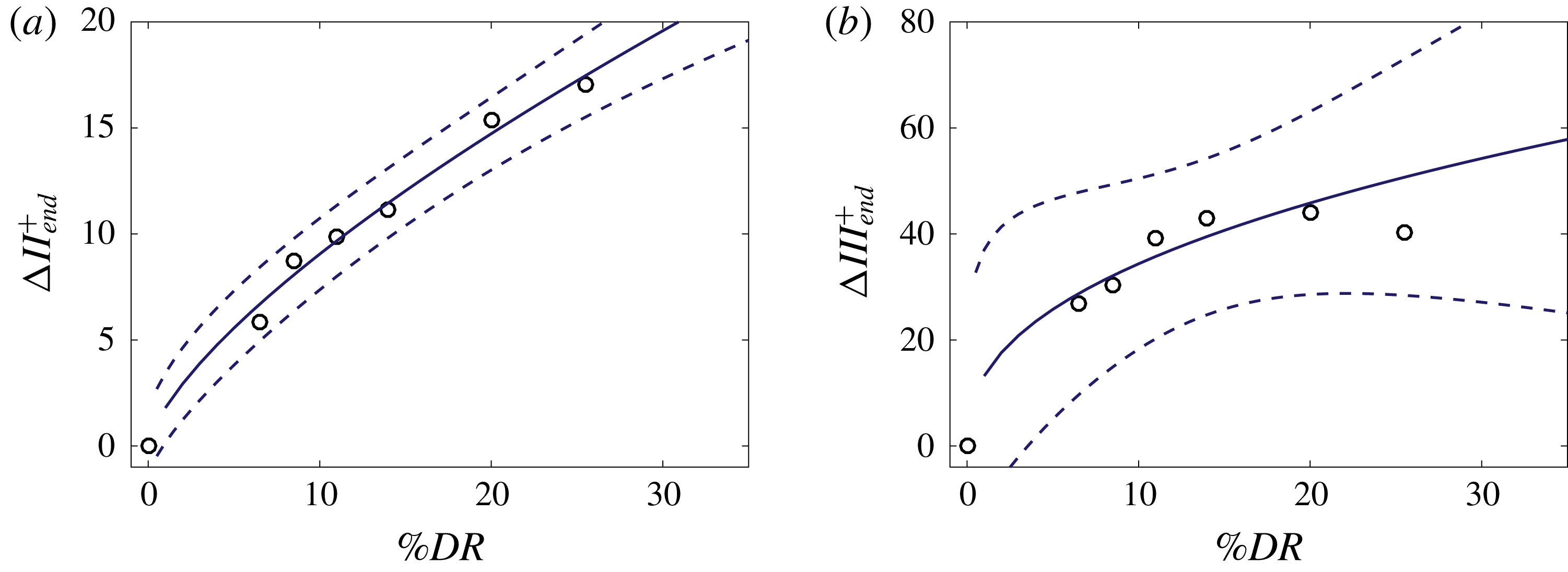
owing to the dynamical influence of the polymer and are presented in figure 23. The scaling for the end point of layer
 $II$
based upon viscoelastic DNS data is estimated as
 ${\sim}2.1\sqrt{\unicode[STIX]{x1D6FF}^{+}}$
. A comparison between experimental data and the scaling for layer
 $II$
are in excellent agreement. For example, at
 $\unicode[STIX]{x1D6FF}^{+}=1463$
, equation (3.11) predicts the end point of layer
 $II$
to occur at
 $y^{+}=79$
, whereas the viscoelastic scaling predicts
 $y^{+}=81$
. Note that the correction for layer
 $III$
has increased uncertainty due to uncertainty in estimating the very small second derivative of
 $U^{+}$
at large
 $y^{+}$
. This effect is clearly reflected in the width of the associated confidence interval shown in figure 23(b). Despite this increased uncertainty, the trend indicated by (3.12) is in accord with recent estimates from lower
 $\unicode[STIX]{x1D6FF}^{+}$
DNS. Specifically, at
 $\unicode[STIX]{x1D6FF}^{+}=1463$
(3.12) prescribes a layer
 $III$
end point near
 $y^{+}=150$
. Consistently, White et al. (Reference White, Dubief and Klewicki2018) used viscoelastic DNS to estimate that layer
 $III$
terminates at
 $y^{+}=4\sqrt{\unicode[STIX]{x1D6FF}^{+}}$
, which for
 $\unicode[STIX]{x1D6FF}^{+}=1463$
gives
 $y^{+}=153$
. Note that even though the corrections agree with viscoelastic DNS data, they are clearly not perfect since these results implicitly assume that the percentage drag reduction and Reynolds number effects are decoupled.
 $$\begin{eqnarray}\displaystyle & \displaystyle II_{end}^{+}=1.6\sqrt{\unicode[STIX]{x1D6FF}^{+}}+1.796(\%DR)^{0.703} & \displaystyle\end{eqnarray}$$
 $$\begin{eqnarray}\displaystyle & \displaystyle III_{end}^{+}=2.6\sqrt{\unicode[STIX]{x1D6FF}^{+}}+13.2(\%DR)^{0.415}. & \displaystyle\end{eqnarray}$$
Corrections to the Newtonian values for the ends of layer
 $II$
(a) and
 $III$
(b) as a function of increasing
 $DR$
at
 $\unicode[STIX]{x1D6FF}^{+}=1800$
, 1691, 1687, 1652, 1592, 1507, 1463. The data are given by
 $\circ$
; the solid lines denote the curve fit; the dashed lines denote a
 $95\,\%$
confidence interval.

With the determination of the layer boundaries, one can then estimate the velocity increments across each layer. Beyond constituting a basic property of the mean dynamical structure, this information has theoretical value relative to, for example, educing the existence of a logarithmic versus power-law mean profile (Wei et al.
Reference Wei, Fife, Klewicki and McMurtry2005). Newtonian flow analysis reveals that the mean velocity increments across layers
 $I$
and
 $III$
scale with
 $u_{\unicode[STIX]{x1D70F}}$
. Conversely, the increment across layer
 $II$
is very close to
 $0.5U_{cl}$
independent of
 $\unicode[STIX]{x1D6FF}^{+}$
, while the increment across layer
 $IV$
approaches
 $0.5U_{cl}$
as
 $\unicode[STIX]{x1D6FF}^{+}\rightarrow \infty$
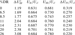
. Table 2 provides velocity increment data from the present experiments. If the increment across layer
 $I$
is taken to be approximately
 $3u_{\unicode[STIX]{x1D70F}}$
, then consistent with previous Newtonian flow analysis, the increment across layer
 $II$
in the Newtonian flow is very close to
 $0.5U_{cl}$
. In agreement with previous quantifications, the measured increment across layer
 $III$
in the
 $DR=0$
case is approximately
 $1.2u_{\unicode[STIX]{x1D70F}}$
. On the other hand, it is apparent that with increasing
 $DR$
the velocity increment from the wall to the outer edges of layer
 $III$
steadily increases. (Interestingly the increment across layer
 $II$
remains nominally fixed.) Nevertheless, the overall observation is that the mean viscous force retains leading order increasingly farther from the wall with increasing drag reduction. Dynamically, this indicates that, on average, more of the total velocity increment (circulation per unit length) is attributable to the region where the
 $TI$
term in (1.3) behaves like a momentum source. Consistent with this, previous measurements of the layer velocity increments in rough-wall flows (Mehdi et al.
Reference Mehdi, Klewicki and White2013) indicate that the increment across the momentum source region decreases with increasing roughness drag. Thus, as a general momentum field diagnostic it would seem that increases in the velocity increment from the wall to the start of layer
 $IV$
, relative to the smooth-wall case, are associated with drag reductions, while decreases in this increment are associated with increasing drag. This has apparent similarity with previous characterizations of drag-reducing flows as behaving like a negative roughness (Hoyt Reference Hoyt1991). Lastly, the relative concentration of velocity increment in layer
 $II$
with increasing
 $DR$
consistently correlates with the aforementioned reduction in
 $\unicode[STIX]{x1D6FF}^{\ast }$
, and apparently supports the notion (analogy) that polymer
 $DR$
promotes a flow structure resembling that found in reverse transition. Further evidence in support of this is that the low-Reynolds-number onset of the four-layer regime correlates with
 $\unicode[STIX]{x1D6FF}^{\ast }$
first exceeding the width of layer
 $II$
(Klewicki Reference Klewicki2013b
).
Velocity increments for layers
 $III$
and
 $IV$
associated with the layer structure of figure 1 at
 $\unicode[STIX]{x1D6FF}^{+}\approxeq 1800$
and for
 $DR>0$
at
 $\unicode[STIX]{x1D6FF}^{+}=1691,1687,1652,1592,1507,1463$
. The velocity at the end points of layers
 $II$
and
 $III$
is also presented.

3.9 Profiles of the momentum transport length,
 $W$

The mean momentum equations for the canonical turbulent wall flows, including (1.2), admit a self-similar structure on two domains (Klewicki Reference Klewicki2013b
). The mathematically simpler of these two is operative on an interior inertial domain. According to the leading-order structure of (1.2) this inertial domain begins near the onset of layer
 $IV$
. Here, analytical treatment of (1.2) reveals that the average size of the momentum transporting motions varies linearly with distance from the wall,
 $y$
(Fife, Klewicki & Wei Reference Fife, Klewicki and Wei2009). On this domain, direct integration of (1.2) yields a similarity solution that asymptotically conforms with the universal logarithmic mean velocity profile (Klewicki & Oberlack Reference Klewicki and Oberlack2015). In accord with the existence of this similarity solution to (1.2), there is a coordinate stretching function that ensures solution invariance for varying
 $\unicode[STIX]{x1D6FF}^{+}$
. This coordinate stretching function is found analytically, denoted by
 $\unicode[STIX]{x1D719}$
, and defined by
 $$\begin{eqnarray}\displaystyle \frac{\text{d}W^{+}}{\text{d}y^{+}}=\unicode[STIX]{x1D719}^{-1}. & & \displaystyle\end{eqnarray}$$
In this expression,
 $W^{+}(y^{+})$
is the continuous distribution of the widths of a self-similar hierarchy of scaling layers termed the
 $L_{\unicode[STIX]{x1D6FD}}$
hierarchy (for example, Klewicki Reference Klewicki2013b
). Formally,
 $W^{+}(y^{+})$
is related to the decay rate of the
 $TI$
term in (1.2). Practically, however,
 $W^{+}$
is most accurately computed using
 $W^{+}=-(\text{d}^{2}U^{+}/\text{d}y^{+2})^{-1/2}$
. Physically, at any location on the
 $L_{\unicode[STIX]{x1D6FD}}$
hierarchy
 $W^{+}$
is the mean length scale of the inertial turbulent motions responsible for the wallward transport of momentum (Klewicki et al.
Reference Klewicki, Philip, Marusic, Chauhan and Morrill-Winter2014). Conceptually,
 $W^{+}$
is similar to von Kármán’s representation of Prandtl’s mixing length. His formulation, however, stems from an intuitive similarity hypothesis, while the properties of
 $W(y)$
are determined from the analysis that determines an invariant representation of the mean dynamical equation that holds on each of the hierarchy layers. Specifically, normalization of the mean momentum equation using
 $u_{\unicode[STIX]{x1D70F}}$
and
 $W$
formally yields a single universal form that holds over the domain where the
 $TI$
term is a decreasing function of
 $y$
, i.e. on the domain of the so-called
 $L_{\unicode[STIX]{x1D6FD}}$
hierarchy. The
 $L_{\unicode[STIX]{x1D6FD}}$
hierarchy domain extends from the inner peak of the
 $TI$
(denoted as
 $y_{pi}^{+}$
) to the outer peak (denoted as
 $y_{po}$
). In Newtonian flow this corresponds to
 $y^{+}=y_{pi}^{+}\approxeq 7$
to
 $y/\unicode[STIX]{x1D6FF}=y_{po}/\unicode[STIX]{x1D6FF}\approxeq 0.5$
, or equivalently between the peak momentum source,
 $y_{pi}^{+}$
, and sink,
 $y_{po}$
, locations (Klewicki, Ebner & Wu Reference Klewicki, Ebner and Wu2011). The portion of the layer hierarchy where the logarithmic similarity solution holds corresponds to the inner part of layer
 $IV$
, where the mean dynamics become inertially dominated and the
 $W^{+}$
profile becomes a linear function of
 $y^{+}$
.
Estimates of the
 $W^{+}$
profiles from the present measurements are displayed in figure 24. It is clear from figure 24 that with increasing
 $DR$
the mean length scale responsible for the transport of momentum is reduced for
 $y^{+}>20$
. Viscoelastic DNS data indicate that for
 $y^{+}<20$
, the mean length scale increases (White et al.
Reference White, Dubief and Klewicki2018). This correlates with a reduction in the intensity of near-wall vorticity stretching. The present data also suggest an increase in
 $W^{+}$
for
 $y^{+}<20$
, but uncertainties in these estimates become significant as the wall is approached.
Profiles of the
 $W^{+}$
layer width distributions as estimated from the present measurements. The solid line is for
 $DR=0$
at
 $\unicode[STIX]{x1D6FF}^{+}\approxeq 1800$
; dashed lines,
 $DR>0$
; dash–dot line, DNS at
 $\unicode[STIX]{x1D6FF}^{+}=2004$
.

When interpreted as a force, the turbulent inertia term in (1.3) behaves like a momentum source for
 $y^{+}<y_{m}^{+}$
, and like a momentum sink for
 $y^{+}>y_{m}^{+}$
(Klewicki et al.
Reference Klewicki, Fife, Wei and McMurtry2007). (Recall that
 $y_{m}^{+}$
is the position where the Reynolds stress attains its maximum, or, equivalently, where
 $TI$
crosses zero.) Owing to
 $$\begin{eqnarray}\displaystyle \int _{0}^{\unicode[STIX]{x1D6FF}}\frac{\text{d}\overline{u^{\prime }v^{\prime }}^{+}}{\text{d}y^{+}}\,\text{d}y^{+}=0, & & \displaystyle\end{eqnarray}$$
the net momentum source and sink contributions sum to zero at any given
 $\unicode[STIX]{x1D6FF}^{+}$
. This integral balance occurs owing to a concentration of smaller, but more intense, source-like motions interior to
 $y_{m}^{+}$
, and larger scale, but less intense, sink-like motions beyond
 $y_{m}^{+}$
. In this regard, Newtonian flow analysis shows that when the
 $TI$
profiles are weighted (premultiplied) by
 $W^{+}$
and plotted on a logarithmic scale, the source and sink contributions to (3.14) appear equally distributed about
 $y_{m}^{+}$
(for example, Klewicki Reference Klewicki2013b
). It is thus useful to investigate this balancing behaviour for drag-reducing flows. The estimate for this profile is given in figure 25(a). Owing to the uncertainty in the present
 $W^{+}$
estimates, it is also useful to compare the weighted total stress gradient profile of figure 25(a) with that employing the pure
 $y$
-scaling surrogate, i.e. the weighted profile,
 $y^{+}\text{d}RPS^{+}/\text{d}y^{+}$
versus
 $y^{+}$
, as was previously employed by Klewicki et al. (Reference Klewicki, Ebner and Wu2011). This profile is shown in figure 25(b). While both of these weighted profiles fail to resolve the peak momentum source near the wall, it is clear that they both consistently indicate that the source contributions to the momentum distribution move farther from the wall in viscous units for
 $DR>0$
flow. In the source region, these profiles also show that the
 $DR>0$
profiles consistently reside above the Newtonian flow profiles. This indicates that the increase in the gradient of the combined polymer and Reynolds stress more than compensates for the observed reduction in the polymer influenced
 $W^{+}$
profiles of figure 24. Unfortunately, the lack of data in the near-wall region does not allow for a precise quantification of these source contributions. Similarly, the
 $W^{+}\text{d}RPS^{+}/\text{d}y^{+}$
profiles show large uncertainties for large
 $y^{+}$
; notice that the profile of figure 25(a) is truncated to only show the inner part of layer
 $IV$
.
Profiles of the weighted
 $W^{+}$
profiles: (a)
 $W^{+}\text{d}RPS^{+}/\text{d}y^{+}$
versus
 $y^{+}$
, (b)
 $y^{+}\text{d}RPS^{+}/\text{d}y^{+}$
versus
 $y^{+}$
. The solid line denotes the
 $DR=0$
profile at
 $\unicode[STIX]{x1D6FF}^{+}\approxeq 1800$
; dashed lines denote
 $DR>0$
cases.

3.10 Rescaling the mean vorticity profile
Further insights are also gained by re-examining the mean vorticity profile within the context of the normalizations predicted by the MMB theory. Specifically, comparison with the
 $DR=0$
channel flow allows for an assessment of the effects of polymer on the establishment and scaling behaviours of the mean vorticity distribution. Here we reiterate that the present channel flow has only one mean vorticity component. This component is parallel to the wall and perpendicular to the flow direction,
 $\unicode[STIX]{x1D6FA}_{z}=-\text{d}U^{+}/\text{d}y^{+}$
, and thus its wall value is directly related to the mean wall shear stress.
Absolute values of the mean vorticity profiles scaled according to the MMB theory by using the inner-normalized peak location,
 $y_{m}^{+}$
, of the
 $RPS^{+}$
as the characteristic scale. The solid line is for
 $DR=0$
at
 $\unicode[STIX]{x1D6FF}^{+}\approxeq 1800$
; dashed lines,
 $DR>0$
; dash–dot line, DNS at
 $\unicode[STIX]{x1D6FF}^{+}=2004$
.

MMB-based analysis of the canonical smooth-wall Newtonian channel flow reveals that the limiting values of the mean vorticity profile can be made the same at any given
 $\unicode[STIX]{x1D6FF}^{+}$
by multiplying
 $|\unicode[STIX]{x1D6FA}_{z}^{+}|$
by
 $\unicode[STIX]{x1D716}^{-1}=\sqrt{(\unicode[STIX]{x1D6FF}^{+})}$
and multiplying
 $y^{+}$
by
 $\unicode[STIX]{x1D716}$
(Klewicki Reference Klewicki2013a
). This scaling is associated with the similarity solution for the mean velocity profile that is formally admitted by the mean momentum equation and that asymptotically underlies the classical logarithmic law (Klewicki & Oberlack Reference Klewicki and Oberlack2015). It exists on the inertial domain that was used in the present estimation of
 $\unicode[STIX]{x1D705}$
in figure 13. An important feature of this solution is that its
 $y$
-coordinate stretching effectively aligns the onset of the inertial domain for all
 $\unicode[STIX]{x1D6FF}^{+}$
. As discussed above relative to the layer velocity increments, at any finite
 $\unicode[STIX]{x1D6FF}^{+}$
slightly more than half of the mean vorticity is contained in the region
 $\unicode[STIX]{x1D716}y^{+}\lesssim 2.6$
, with the remainder being spread over a layer
 $IV$
domain that approaches
 $\unicode[STIX]{x1D6FF}$
in width as
 $\unicode[STIX]{x1D6FF}^{+}\rightarrow \infty$
(Klewicki Reference Klewicki2013a
). A key finding of the canonical flow analysis is that from the MMB one can analytically surmise that the inner-normalized widths of layers
 $II$
and
 $III$
, as well as
 $y_{m}^{+}$
, all scale like
 $\sqrt{\unicode[STIX]{x1D6FF}^{+}}$
. Relative to non-canonical flows, Mehdi et al. (Reference Mehdi, Klewicki and White2013) were the first to hypothesize that when the four-layer structure depicted in figure 1 is qualitatively retained, the same scaling framework will remain operative. Here we note that figure 22 clearly reveals that this is the present case. Physically, this indicates that the flow structure retains the same characteristic balance exchange of mean forces across layer
 $III$
(leading to an inertially dominated layer
 $IV$
), as well as the associated change from a momentum source to momentum sink-like behaviour of the non-viscous stress gradients across layer
 $III$
. Under such cases, however, the characteristic scale (analogous to
 $\unicode[STIX]{x1D716}$
) must generally be determined empirically. In this regard,
 $y_{m}^{+}$
provides a convenient and physically equivalent surrogate scale, and rough-wall experiments provide clear evidence that
 $y_{m}^{+}$
effectively recovers the invariant scaling for
 $|\unicode[STIX]{x1D6FA}_{z}|$
described above (Mehdi et al.
Reference Mehdi, Klewicki and White2013; Ebner et al.
Reference Ebner, Mehdi and Klewicki2016; Squire et al.
Reference Squire, Morrill-Winter, Hutchins, Schultz, Klewicki and Marusic2016).
The scaling recipe just described is applied to the present polymer data in figure 26. In this figure the absolute value of the inner-normalized mean vorticity is weighted by
 $y_{m}^{+}$
, the inner-normalized position of the peak in the
 $RPS$
, and similarly
 $y^{+}$
is divided by
 $y_{m}^{+}$
. As is apparent, interior to
 $y^{+}/y_{m}^{+}\simeq 3$
, the polymer-influenced profiles clearly diverge from those for Newtonian flow. Specifically, with increasing
 $DR$
the profiles in this region consistently shift upwards, and then merge with or cross over the Newtonian profile closer to the wall. A similar trend occurs for decreasing
 $\unicode[STIX]{x1D6FF}^{+}$
in Newtonian flow. This is, therefore, interpreted to provide further support that polymer drag reduction has an effect that, in a number of respects, is similar to that of reducing the Reynolds number (White et al.
Reference White, Dubief and Klewicki2018). Beyond
 $y^{+}/y_{m}^{+}\simeq 3$
, the
 $DR=0$
and all of the
 $DR>0$
profiles in figure 26 are nearly indistinguishable. Note, however, that the Newtonian and lower
 $DR$
profiles tend towards coalescence along a straight line (
 $-1$
power law) progressively closer to the wall with decreasing
 $DR$
. The
 $y^{+}/y_{m}^{+}\simeq 3$
position approximately denotes the outer edge of layer
 $III$
for the highest
 $DR$
case. Thus, per the MMB theory, this corresponds to the onset of the inertial sublayer for this flow. Overall, the results of figure 26 are taken to provide compelling support for the present MMB-based theoretical description and the concomitant scaling prescriptions for the mean vorticity profile. They also corroborate the present means for identifying the inertial layer bounds used to estimate the value of
 $\unicode[STIX]{x1D705}$
. Lastly, it is relevant to note that for the flows indicated in figure 26 the position
 $y^{+}/y_{m}^{+}\simeq 3$
is also quite close to
 $y^{+}=4\sqrt{\unicode[STIX]{x1D6FF}^{+}}$
, and thus these results are also consistent with the recent estimate of White et al. (Reference White, Dubief and Klewicki2018) for the inertial layer onset for
 $DR>0$
.
3.11 Diagnostic plot
As described in § 3.9, the MMB can be transformed into a single parameter-free form that is valid across a continuous hierarchy of scaling layers. The width distribution of these layers,
 $W^{+}(y^{+})$
, is an increasing function of wall-normal distance that in Newtonian flow spans
 $4\lesssim W^{+}\lesssim \unicode[STIX]{x1D6FF}^{+}/3$
over
 $7\lesssim y^{+}\lesssim \unicode[STIX]{x1D6FF}^{+}/2$
. For the part of the layer hierarchy on the inertial domain (
 $2.6\sqrt{\unicode[STIX]{x1D6FF}^{+}}\lesssim y^{+}\lesssim \unicode[STIX]{x1D6FF}^{+}/2$
) the self-similar structure of the MMB is characterized by
 $W^{+}\propto y^{+}$
; a condition that becomes exact as
 $\unicode[STIX]{x1D6FF}^{+}\rightarrow \infty$
. A logarithmic mean velocity profile stems from this self-similar structure. Zhou & Klewicki (Reference Zhou and Klewicki2015) investigated the correspondences between the self-similar inertial domain just described, and that found for other measures of self-similar structure in the canonical boundary layer. Notably, to within the uncertainty of their data they found an exact correspondence between
 $2.6\sqrt{\unicode[STIX]{x1D6FF}^{+}}\lesssim y^{+}\lesssim \unicode[STIX]{x1D6FF}^{+}/2$
and the domain over which the so-called diagnostic plot of Alfredsson, Orlu & Segalini (Reference Alfredsson, Orlu and Segalini2012) exhibits its (approximately) linear decrease.
Versions of the diagnostic plot. Streamwise r.m.s. velocity normalized with
 $U(y)$
versus
 $U(y)$
normalized by (a)
 $U_{cl}$
and (b)
 $U$
velocity at the end of layer
 $III$
,
 $U_{III}$
. See figure 26 and caption for line definitions. Symbols in (a) denote position of the onset of layer
 $IV$
for each profile, and the vertical line denotes the value of
 $U/U_{cl}$
at the end of layer
 $III$
in the DNS
 $DR=0$
flow at
 $\unicode[STIX]{x1D6FF}^{+}=2004$
.

Originally developed as a means to identify data anomalies in the near-wall profile of
 $\sqrt{\overline{u^{\prime 2}}}$
, the diagnostic plot represents the r.m.s.
 $u^{\prime }$
normalized by the corresponding
 $U$
value versus
 $U/U_{cl}$
(Alfredsson et al.
Reference Alfredsson, Orlu and Segalini2012). In this regard,
 $U/U_{cl}$
acts as a flow structure based surrogate for the normalized distance from the wall. This representation of the diagnostic plot is given in figure 27(a). Referencing the Newtonian fluid flow cases (
 $\unicode[STIX]{x1D6FF}^{+}\approxeq 1800$
experiment,
 $\unicode[STIX]{x1D6FF}^{+}=2004$
DNS), it is apparent that these profiles complete their distinct change in slope near
 $U/U_{cl}=0.68$
at the present
 $\unicode[STIX]{x1D6FF}^{+}$
. As observed by Zhou & Klewicki (Reference Zhou and Klewicki2015) in boundary layers over
 $1450\leqslant \unicode[STIX]{x1D6FF}^{+}\leqslant 19\,600$
this knee in the curve slowly moves to lower
 $U/U_{cl}$
with increasing
 $\unicode[STIX]{x1D6FF}^{+}$
, and the onset of the Reynolds-number-invariant (approximately linear) region closely corresponds to the start of the inertial domain found from consideration of the MMB. For the DNS, this position is denoted by the solid vertical line in figure 27(a), and by the black diamond symbol for the
 $\unicode[STIX]{x1D6FF}^{+}\simeq 1800$
experiment. Similarly, the coloured symbols denote the onset of layer
 $IV$
for each of the
 $DR>0$
cases. For increasing
 $DR$
it is apparent that these marked positions successively coincide with where the
 $DR>0$
profiles nominally merge with the
 $DR=0$
profiles. In contrast to the present drag-reduced flow, the roughness study by Castro, Segalini & Alfredsson (Reference Castro, Segalini and Alfredsson2013) indicates that roughness shifts the profiles above the Newtonian case, whereas the shift is below for
 $DR>0$
(
 $U/U_{cl}<0.5$
), as shown in figure 27(a). Similarly, 27(b) uses the normalization
 $U/U_{III}$
(see table 2) to illustrate that all of the curves do indeed begin their shallower slope near
 $U/U_{III}=1$
. These profiles also clearly reveal that, relative to the invariant
 $DR=0$
profile slope, the
 $DR>0$
profiles exhibit a continuous variation with increasing
 $DR$
. Overall, the results of figure 27 provide clear evidence that, with increasing
 $DR$
, the inertial sublayer continuously moves outwards in
 $y^{+}$
, its width diminishes, and the invariant
 $DR=0$
relationship between
 $\sqrt{\overline{u^{\prime 2}}}$
and
 $U$
on the inertial sublayer continuously changes. Note, however, that this analysis relies on the empirical observation that the scaling domain for the diagnostic plot coincides with the bounds of the inertial domain as determined from the MMB theory. Thus it is a correlative finding, as opposed to an analytical result.
4 Conclusions
A number of physical interpretations of the present measurements were discussed in the preceding narrative, and thus are not repeated here. This section instead first summarizes the primary empirical observations. It then concludes with a comparative discussion (relative to the
 $DR=0$
case) of how drag-reducing polymers influence the establishment of the mean momentum field and modify the vortical structure of the flow.
The present results reveal clear effects associated with increasing
 $DR$
at fixed
 $\unicode[STIX]{x1D6FF}^{+}$
on a number of statistical quantities. This includes compelling evidence that, for the
 $DR$
range explored, the mean profile slope on the inertial sublayer (as reflected by the inverse of
 $\unicode[STIX]{x1D705}$
) undergoes an essentially continuous and approximately linear increase with
 $DR$
(figure 14). Similarly, the peak value and peak position of the r.m.s.
 $u^{\prime }$
(figure 18), the maximum value and
 $y^{+}$
position of the
 $RPS$
(figure 21), and the reduction in
 $\unicode[STIX]{x1D6FF}^{\ast }$
(figure 10), also vary approximately linearly with
 $DR$
. On the other hand, evidence was provided (figures 17 and 20) indicating that the relationship between the injected polymer concentration and the level of drag reduction is nonlinear.
Schematic depiction of vorticity field attributes in (a) canonical flows and (b) polymer
 $DR$
flows, adapted from Klewicki (Reference Klewicki2013a
). Note that the horizontal scale (distance from the wall) is stretched, nominally logarithmic; for example, in the Newtonian flow layer
 $II$
is only approximately
 $1.6$
times larger than layer
 $III$
. Velocity field motions (light grey) are space-filling throughout. Owing to vorticity stretching the vortically intense motions (hatched) begin to become spatially intermittent in layer II, and on the inertial domain (layer
 $IV$
) spatially disperse. In polymer
 $DR$
flows, the layer
 $II$
vorticity stretching is diminished, and the vortical motions on both layers
 $II$
and
 $IV$
are more space-filling than in the
 $DR=0$
case.

Analyses of canonical wall flows reveal that the mean momentum equation admits a parameter-free form that properly reflects the leading balance of forces as a function of distance from the wall, and that is invariant across a self-similar hierarchy of scaling layers (Klewicki Reference Klewicki2013b
). Distance-from-the-wall scaling on the inertial domain is an analytical result that derives from this structure, as is a logarithmic mean profile equation. In accord with the findings of White et al. (Reference White, Dubief and Klewicki2018), the present measurements provide evidence that this self-similar structure is modified as a function of
 $DR$
and
 $\unicode[STIX]{x1D6FF}^{+}$
. Perhaps the clearest evidence of this is the essentially continuous variation in
 $\unicode[STIX]{x1D705}$
for
 $DR>0$
. That is, from the canonical flow analysis,
 $\unicode[STIX]{x1D705}$
is known to have a direct relationship to the coordinate stretching function
 $\unicode[STIX]{x1D719}$
(i.e.
 $\unicode[STIX]{x1D705}=\unicode[STIX]{x1D719}^{-2}$
) that underlies the invariant form of the mean dynamical equation on the inertial subdomain of the scaling layer hierarchy. In concert with the recent findings of White et al. (Reference White, Dubief and Klewicki2018) and relative to the modified structure observed herein, figure 28(a) depicts the canonical flow structure, and figure 28(b) depicts our interpretation of the influence of drag-reducing polymer. These figures show representations of the space-filling properties of, and scale separation between, the velocity and vorticity field motions with distance from the wall (horizontal axis). These (on average) cartoons of instantaneous structure are a companion to the mean vorticity profiles of figure 26. As indicated in figure 28(b), our collective findings suggest that a primary effect of polymer is that it limits near-wall vorticity stretching and reorientation, and thus attenuates/delays the three-dimensionalization of the vorticity field in layer
 $II$
that would otherwise occur. This connects to the observed onset of the inertial layer at larger
 $y^{+}$
, an increase in the scale of the organized vortical motions, and, as a result, a reduction in the overall scale separation on the inertial domain. Indeed, while the vortical fissures on the inertial layer are depicted on this cartoon as distinct, the instantaneous vortical motions are expected to become increasingly diffuse with increasing
 $DR$
. This gradual loss of scale separation on the inertial domain is quite naturally associated with the numerous observations that the effect of polymer is to move the flow state towards reverse transition, and similarly, the continuous inertial layer variation of the
 $\sqrt{\overline{u^{\prime 2}}}/U$
profiles shown in figure 27.
Lastly, it is similarly worth revisiting the aforementioned notion that polymer
 $DR$
acts, in a number of ways, like a ‘negative roughness’ (Hoyt Reference Hoyt1991). Here it is noted that the action of roughness is to generally augment drag. A symptom of this is that the layer
 $II$
three-dimensionalization of the vorticity field is also augmented, and accordingly, there is a more rapid development of inertial mean dynamics with distance from the wall (Ebner et al.
Reference Ebner, Mehdi and Klewicki2016). As just noted, these effects are opposite those associated with polymer
 $DR$
. Accordingly, this more rapid development of inertial mean dynamics is accompanied by a relative reduction in the mean velocity increment interior to layer
 $IV$
. Thus, the drag increase associated with roughness correlates with an increased velocity increment on the domain where the turbulent inertia behaves like a momentum sink. Consistent with the negative roughness analogy, the present
 $DR>0$
cases reveal a relative increase in the velocity increment on the momentum source side of
 $y_{m}$
. Overall, the attributes just noted are likely to reflect generic signatures of a net drag augmentation versus a net drag reduction.
Acknowledgements
This study was supported by Australian Research Council grants DP120101467 and LE130100088.