1 INTRODUCTION
Consider the semiparametric linear regression model

where
$y \in \mathbb {R}$
 is the outcome variable,
$x \in \mathbb {R}^{d_x}$
 is the treatment vector of interest,
$z_{1} \in \mathbb {R}^{d_{z_{1}}}$
 is a vector of controls, and
$\varepsilon $
 is an unobserved disturbance. A common assumption in Bayesian analysis is that the regressors x are exogenous, meaning that they are uncorrelated with the error term
$\varepsilon $
 . In many empirical settings, this assumption is questionable. If one has access to a set of valid instruments
$z_{2} \in \mathbb {R}^{d_{z_{2}}}$
 , with dimension at least as large as that of x, it becomes possible to conduct a Bayesian analysis that correctly accounts for endogeneity. Such analysis can be formulated within both parametric and semiparametric frameworks, as in the early contributions of Drèze (Reference Drèze1976) and the subsequent developments in Kleibergen and van Dijk (Reference Kleibergen and van Dijk1998), Chao and Phillips (Reference Chao and Phillips1998), Kleibergen and Zivot (Reference Kleibergen and Zivot2003), and Schennach (Reference Schennach2005), among many others. Recent work, including Hoogerheide, Kleibergen, and van Dijk (Reference Hoogerheide, Kleibergen and van Dijk2007), Liao and Jiang (Reference Liao and Jiang2011), Florens and Simoni (Reference Florens and Simoni2012), Florens and Simoni (Reference Florens and Simoni2016), Florens and Simoni (Reference Florens and Simoni2021), Kato (Reference Kato2013), Shin (Reference Shin2014), and Chib, Shin, and Simoni (Reference Chib, Shin and Simoni2018), has extended these ideas to semiparametric and likelihood-free settings.
An important question that has received little attention in the Bayesian literature concerns the testing of endogeneity. Frequentist methods, such as the classical Durbin–Wu–Hausman test, offer an asymptotic procedure that assesses exogeneity by comparing estimators that are consistent under different assumptions. These procedures, however, do not translate naturally into the Bayesian framework. From a Bayesian standpoint, it is more straightforward to conceptualize the test for endogeneity as a comparison of models, rather than that of parameters. Specifically, one can develop a test that is based on the relative support provided by the data for a model with exogeneity versus a model with endogeneity.
To develop this approach, and to avoid distributional assumptions, we proceed within a Bayesian framework for moment condition models. We consider two competing specifications. The first is a base model defined by the moment conditions

where
$\varepsilon (\theta ) := y - x^{\prime }\beta - z_{1}^{\prime }\gamma $
 and
$\theta := (\beta ,\gamma )$
 . The second is an extended model that relaxes the exogeneity restriction and allows

where v captures the covariance between the error term and the endogenous variable x. We formulate the prior–posterior analysis of each model through the nonparametric exponentially tilted empirical likelihood (ETEL) and then compare the two models by marginal likelihoods and the Bayes factor. This approach offers several methodological advantages. The Bayes factor measures the strength of evidence for the two models on a continuous scale rather than through a strict accept or reject rule. In addition, the use of ETEL provides robustness to misspecification of the joint distribution of
$(y, x, z_1, z_2)$
 and allows us to obtain results that remain valid without specifying the distribution of the disturbances.
Using the Chib (Reference Chib1995) marginal likelihood identity, we know that the log marginal likelihood decomposes into three parts: the log ETEL, the log prior, and the negative log posterior ordinate. We establish that this expression is asymptotically equal to a term bounded in probability, plus a term proportional to the Kullback–Leibler (KL) divergence between the true and the closest probability distribution satisfying the moment restrictions term, plus a penalty that corresponds to the ones of the Bayesian information criterion (BIC). The penalty arises from a change-of-variable transformation of the posterior density evaluated at the true or pseudo-true value of the parameters. The log of the Jacobian of this transformation constitutes the penalty, while the posterior density of the local parameter at zero is bounded in probability as n increases. Accordingly, when x is exogenous, the log-ETELs of the two models are asymptotically the same but the penalties differ. When x is endogenous, the difference in the log-ETELs dominates, which leads to the selection of the extended model. Thus, the test correctly discriminates between the two data-generating processes (DGPs) in large samples. Our construction parallels the logic of the Hausman test, where one compares an estimator that is inconsistent under endogeneity with one that is not. Here, the comparison is between models that differ in the number of overidentifying moment conditions. In this sense, our test may be viewed as the Bayesian analog of the Hausman specification test.
Compared to Chib et al. (Reference Chib, Shin and Simoni2018), our work builds on the same Bayesian ETEL framework but makes several key contributions. First, while Chib et al. (Reference Chib, Shin and Simoni2018) explains how to test among different models, it does not address how to construct the specific models required to test hypotheses of interest in practical applications, such as the endogeneity problem we examine here. In this article, we explicitly construct the models necessary for testing endogeneity. Second, we introduce an assumption that guarantees the existence of the ETEL function, which, to our knowledge, is absent from the existing ETEL literature. This assumption ensures that the ETEL function exists at least in a suitable neighborhood of the true parameter value with probability approaching 1. The issue arises because the ETEL function, as the solution to a constrained optimization problem, may have an empty feasible set for certain parameter values
$\theta $
 . Without this assumption, derivatives of the ETEL function cannot be defined, posing challenges for both frequentist and Bayesian ETEL approaches. Third, we provide a more direct proof demonstrating that the ETEL function is asymptotically equivalent to a quadratic function. This result underpins our establishment of a Bernstein–von Mises theorem, which we then use to prove the consistency of our testing procedure. The direct proof leverages the linearity in
$\theta $
 of the moment restrictions implied in the instrumental variable (IV) regression problem. Along the same lines, the assumptions in this article are weaker than those in Chib et al. (Reference Chib, Shin and Simoni2018), as they exploit the IV linear regression structure.
Finally, as a by-product of proving the consistency of our testing procedure, we derive a new asymptotic representation of the log-marginal ETEL function, defined as the ETEL function integrated with respect to the prior distribution of the model parameter. We show that the log-marginal likelihood of each model can be asymptotically decomposed into a KL divergence term (between the true distribution and the closest distribution satisfying the model’s moment restrictions) plus a BIC-type penalty. We derive this penalty using a novel approach: by re-expressing the posterior ordinate at the true (or pseudo-true) parameter value via a local parameter change of variables, the resulting log-Jacobian yields the penalty term, while the posterior density of the local parameter evaluated at zero is
$\mathcal {O}_{p}(1)$
 as
$n\rightarrow \infty $
 . This representation clarifies the mechanics of Bayes-factor testing in this context and leads to a more transparent proof of model-selection consistency than that in Chib et al. (Reference Chib, Shin and Simoni2018). Notably, we emphasize that the penalty plays a role in selecting the correct model only when x is exogenous, in which case both models are correctly specified.
The rest of the article proceeds as follows. Section 2 summarizes Bayesian estimation and comparison of moment condition models using ETEL. Section 3 presents the base and extended models and provides a simulated example to illustrate the procedure. Section 4 develops the test for endogeneity and analyzes the large-sample behavior of the log-marginal likelihood, establishing consistency of the test. Section 5 presents empirical examples, and Section 6 concludes. Appendix A contains the proofs of the main results while the remaining proofs and additional theoretical results are in the Supplementary Material. The latter also contains comparative analysis for model selection, extended simulations, and computational guidance.
2 PRELIMINARIES
In this section, we briefly provide the background on Bayesian estimation of moment condition models using the ETEL. Further details can be found in Schennach (Reference Schennach2005) and Chib et al. (Reference Chib, Shin and Simoni2018).
2.1 Moment Restrictions and Feasible Distributions
Let
$w\in \mathbb {R}^{d_w}$
 be a random vector, and let
$\theta \in \Theta \subset \mathbb {R}^{p}$
 denote a generic parameter vector. Let
$\mathbb {M}$
 denote the set of all probability distributions on
$\mathbb {R}^{d_w}$
 . For a known vector of moment functions,

the moment restriction is given by

where
$Q\in \mathbb {M}$
 is a probability distribution under which the restriction is imposed and
$\mathbf {E}^Q[\cdot ]$
 denotes the expectation under Q. For each
$\theta \in \Theta $
 , define the subset of distributions that satisfy the moment restriction by

Suppose the data
$w_{1:n}:=(w_{1},\ldots ,w_{n})$
 are independently drawn from the true distribution P, which need not belong to
$\mathcal {Q}(\theta )$
 for some
$\theta \in \Theta $
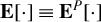
 . The expectation taken with respect to the true distribution P is denoted by
$\mathbf {E}[\cdot ] \equiv \mathbf {E}^P[\cdot ]$
 .
2.2 Sample ETEL Weights, Tilted Sample Distribution, and Likelihood
The empirical counterpart of (2.1) is the weighted restriction

where
$\{q_i\}_{i=1}^n$
 is a discrete distribution supported on
$\{w_i\}_{i=1}^n$
 . Equivalently, any such weight vector induces a discrete probability measure on
$\mathbb {R}^{d_w}$
 with support
$\{w_1,\ldots ,w_n\}$


where
$\delta _{w_i}$
 denotes the point mass at
$w_i$
 .
Since there might be no
$\theta \in \Theta $
 such that the uniform empirical distribution
$q_i\equiv 1/n$
 satisfies (2.3), we define the ETEL weights as the solution to the following KL-closest feasible reweighting problem:

which depends on the parameter vector
$\theta \in \Theta $
 . Let
$H_n\subset \Theta $
 be the set of
$\theta $
 values for which the program (2.5) is feasible, that is, the set of
$\theta $
 s such that the interior of the convex hull of
$\{g(w_{i},\theta ): i=1,\ldots ,n\}$
 contains zero. Assumption 3 below ensures that
$H_n$
 is non-empty with probability approaching
$1$
 .
For
$\theta \in H_n$
 , the ETEL (sample likelihood) is defined as the product of the ETEL weights

The ETEL arises as the integrated likelihood obtained by integrating out the unknown distribution Q with respect to a particular nonparametric prior that imposes the moment restrictions (2.3) conditional on a
$\theta \in H_n$
 (see Schennach, Reference Schennach2005).
Given a prior density
$\pi (\theta )$
 , the ETEL-based posterior is the truncated posterior

where
$I[A]$
 denotes the indicator function. Since (2.6) is not available in closed form, posterior summaries are obtained via tailored Markov chain Monte Carlo (MCMC) methods. Section C of the Supplementary Material describes computational details on MCMC sampling and related calculations.
2.3 Dual Representation and Log-ETEL Identities
A convenient way to compute
$\{\widehat {q}_{i}(\theta )\}$
 is via the dual representation of (2.5). Define the ETEL multiplier as, for every
$\theta \in H_n$
 ,

Then, for every
$\theta \in H_n$
 ,

It is useful to view (2.7) as an exponential tilting of the uniform empirical distribution
$P_n(\cdot ) := \frac {1}{n}\sum _{i=1}^n \delta _{w_i}(\cdot )$
 , which places mass
$1/n$
 on each observation. For fixed
$\theta \in H_n$
 , the ETEL weights
$\{\widehat q_i(\theta )\}$
 therefore define a tilted sample distribution

that is, absolutely continuous with respect to
$P_n$
 . In particular, for each support point
$w_i$
 ,

so
$\widehat Q_n(\cdot \mid \theta )$
 is the exponential tilt of
$P_n$
 that enforces the sample moment restriction (2.3). The multiplier
$\widehat \lambda (\theta )$
 satisfies the sample first-order condition

which is the sample analog of (2.1) under the ETEL weights. For later use, we record the log-ETEL in a form amenable to expansions. Summing
$\log \widehat q_i(\theta )$
 yields the exact identity

or equivalently,

2.4 Population KL Projection, Exponential Tilting, and Pseudo-True Values
The population counterpart of
$\{\widehat {q}_{i}(\theta )\}_{i=1}^n$
 is the distribution
$Q^*(\theta )\in \mathcal {Q}(\theta )$
 that is the closest to P in the KL divergence. For each
$\theta $
 such that
$\mathcal {Q}(\theta ) \neq \emptyset $
 , define

where

if Q is absolutely continuous with respect to P, and
$\mathrm {KL}(Q||P) = +\infty $
 , otherwise. The population counterpart of the ETEL multiplier
$\widehat {\lambda }(\theta )$
 is

for every
$\theta \in \Theta $
 such that
$\mathcal {Q}(\theta ) \neq \emptyset $
 . This induces the population exponential tilt

Under mild regularity conditions, the KL projection
$Q^*(\theta )$
 admits the Radon–Nikodym derivative representation

Thus, if P admits a Lebesgue density
$p(w)$
 , then
$Q^*(\theta )$
 has density given by an exponential tilt of
$p(w)$
 :

By a change of measure,

The right-hand side is the population tilted moment condition. It is the moment restriction expressed under P rather than under
$Q^*(\theta )$
 . If one or more moment conditions are misspecified, then
$Q^*(\theta )\neq P$
 for all
$\theta \in \Theta $
 , and the pseudo-true value
$\theta _*$
 is defined as the minimizer of the reversed KL divergence

where

whenever P is absolutely continuous with respect to
$Q^*(\theta )$
 . Under correct specification, there exists
$\theta _\circ \in \Theta $
 such that
$P\in \mathcal {Q}(\theta _\circ )$
 , in which case
$Q^*(\theta _\circ )=P$
 and
$\theta _* = \theta _\circ $
 . Moreover, in that case
$\lambda _*(\theta _\circ )=0$
 and hence
$q(w;\theta _\circ )\equiv 1$
 . Finally, when the dual representation holds, the pseudo-true value
$\theta _*$
 may also be expressed in terms of the population tilt as

where the term inside the logarithm is the Radon–Nikodym derivative
$[dQ^*(\theta )/dP](w)$
 in (2.14).
3 MODELS
In this section, we specialize the generic moment-restriction framework in Section 2 to the semiparametric linear regression setting introduced in Section 1.
3.1 Data, Regression Structure, and Target Parameter
Let
$w:=(y,x,z_{1},z_{2})\, \in \mathbb {R}^{d+1}$
 be distributed according to an unknown probability distribution P, where
$d := d_{x}+d_{z_{1}}+d_{z_{2}}$
 and
$d_w = d + 1$
 . Throughout,
$\mathbf {E}[\cdot ]:=\mathbf {E}^{P}[\cdot ]$
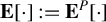 denotes expectation under P. We assume that under P, the random vector w follows the regression model

where
$\theta _{\circ }:=(\beta _{\circ },\gamma _{\circ })\in \Theta \subset \mathbb {R}^p$
 is the true value of the regression coefficients, viewed as a functional of P:
$\theta _{\circ } \equiv \theta _{\circ }(P)$
 and
$p=d_{x}+d_{z_{1}}$
 . In model (3.1), the vector
$z_{1}$
 contains exogenous controls (including an intercept), and
$z_{2}$
 contains IVs. The object of interest is the causal effect of x on y, represented by
$\beta _{\circ }$
 . For any
$\theta := (\beta ',\gamma ')'\in \Theta \subset \mathbb {R}^p$
 , with
$p=d_{x}+d_{z_{1}}$
 and
$\widetilde {w}_1 := (x',z_1')'$
 , define the regression residual

If x is endogenous under P, then
$\mathbf {E}[\varepsilon (\theta _\circ )x]\neq 0$
 . When
$d_{z_2}\geq d_x$
 , the instruments
$z_2$
 help identify
$\beta _\circ $
 despite endogeneity.
3.2 Base Model
$\mathcal {M}_b$
 (Possibly Misspecified)

The base model, denoted by
$\mathcal {M}_b$
 , imposes the moment restrictions

where the base-model moment function is

and the set of distributions satisfying the base-model restrictions is

Here,
$\mathbb {M}$
 denotes the set of all probability distributions on
$\mathbb {R}^{d+1}$
 . Under exogeneity,
$\mathbf {E}[\varepsilon (\theta _\circ )x]=0$
 and the true distribution P satisfies the base-model moments at
$\theta _\circ $
 , so that
$P\in \mathcal {Q}_b(\theta _\circ )$
 . Under endogeneity,
$\mathbf {E}[\varepsilon (\theta _\circ )x]\neq 0$
 and therefore
$P\notin \mathcal {Q}_b(\theta )$
 for every
$\theta \in \Theta $
 ; in that case,
$\mathcal {M}_b$
 is misspecified. In this case, the ETEL function, constructed from the sample
$w_{1:n}$
 , is the empirical counterpart of the distribution
$Q_{b}^{*}(\theta )$
 that for every
$\theta $
 solves the moment conditions:

and that is the closest to P in the KL divergence among all the distributions in the set
$\mathcal {Q}_{b}(\theta )$
 , that is,

Notice that
$\mathrm {KL}(Q\Vert P)$
 is set to
$+\infty $
 , if Q is not absolutely continuous with respect to P. In addition,

denotes the pseudo-true value in the base model. Assumption 1 given in Section 4.5 below guarantees that this value exists. On the other hand, if x is exogenous, then
$Q_{b}^{\ast }(\theta _{\ast })=P$
 and
$\theta _* = \theta _\circ $
 , where
$\theta _\circ $
 denotes the true value of
$\theta $
 as defined above. In the following, we denote the ETEL for the base model by
$\widehat {q}(w_{1:n}|\theta ,\mathcal {M}_b) := \prod _{i=1}^n \widehat {q}_i(\theta |\mathcal {M}_b)$
 , where
$\widehat {q}_i(\theta |\mathcal {M}_b)$
 is constructed as in (2.5) with
$g(w_i,\theta )$
 replaced by
$g_{b}(w_i,\theta )$
 .
3.3 Extended Model
$\mathcal {M}_e$
(Correctly Specified)

The extended model, denoted by
$\mathcal {M}_e$
 , augments the base model by explicitly parameterizing the endogeneity component

Let
$\mathcal {V}\subset \mathbb {R}^{d_x}$
 and define the extended parameter

The extended-model moment function is

and the model imposes the moment restrictions

where

By construction,
$\mathcal {M}_e$
 is correctly specified under both exogeneity and endogeneity of x. Indeed, let

Under (3.1), we have
$\mathbf {E}[\varepsilon (\theta _\circ )z_1]=0$
 and
$\mathbf {E}[\varepsilon (\theta _\circ )z_2]=0$
 , and therefore,

Consequently,
$P\in \mathcal {Q}_e(\psi _\circ )$
 and the KL projection satisfies

In the extended model, the minimizer,
$Q_{e}^{\ast }(\psi )=\arg \inf _{Q\in \mathcal {Q}_{e}(\psi )} \mathrm {KL}(Q\Vert P)$
 , is equal to P, and the population moment conditions in the extended model are

Moreover,

where
$\lambda _*(\psi ):=\arg \min _{\lambda \in \mathbb {R}^{d}}\mathbf {E}[e^{\lambda ^{\prime }g_{e}(w,\psi )}]$
 for every
$\psi \in \mathcal {V}$
 such that
$\mathcal {Q}_e(\psi )\neq \emptyset $
 . In the following, we denote the ETEL for the extended model by
$\widehat {q}(w_{1:n}|\theta ,\mathcal {M}_e) := \prod _{i=1}^n \widehat {q}_i(\theta |\mathcal {M}_e)$
 , where
$\widehat {q}_i(\theta |\mathcal {M}_e)$
 is constructed as in (2.5) with
$g(w_i,\theta )$
 replaced by
$g_{e}(w_i,\psi )$
 .
3.4 Numerical Illustration
To illustrate the fitting of the base and extended models, consider first the base model under endogeneity. Let the DGP be

for
$i=1,\ldots ,n$
 , where
$n\in \{250,500,1,000,2,000\}$
 . Suppose that the
$ (u_{i},v_{i},\omega _{i})$
 are marginally Gaussian, that
$\varepsilon _{i}$
 is marginally a skewed Gaussian mixture
$0.5\mathcal {N}(0.5,0.5^{2})+0.5 \mathcal {N}(-0.5,1.118^{2})$
 , that
$(\varepsilon _{i},u_{i},v_{i})$
 have a joint distribution induced by a Gaussian copula with covariance matrix
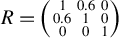 and that the covariance of
$\omega _{i}$
 with each of the other errors is zero. Also assume that each parameter is 1 (except for
$ \delta _{1}$
 , which is 0.5). Under this DGP,
$z_{1i}$
 is uncorrelated with
$ \varepsilon _{i}$
 and correlated with
$x_{i}$
 but since
$\omega _{i}$
 is uncorrelated with the other shocks,
$z_{2i}$
 is a valid instrument that is also relevant for
$x_{i} $
 . For each of the four sample sizes, the posterior of
$\theta :=(\beta ,\gamma _{0},\gamma _{1})$
 is calculated from the four moment conditions

The ETEL posterior is sampled by the tailored one-block Metropolis–Hastings (M–H) algorithm (Chib and Greenberg, Reference Chib and Greenberg1995) for 20,000 iterations beyond a burn-in of 1,000 cycles. The marginal posterior density of
$\beta $
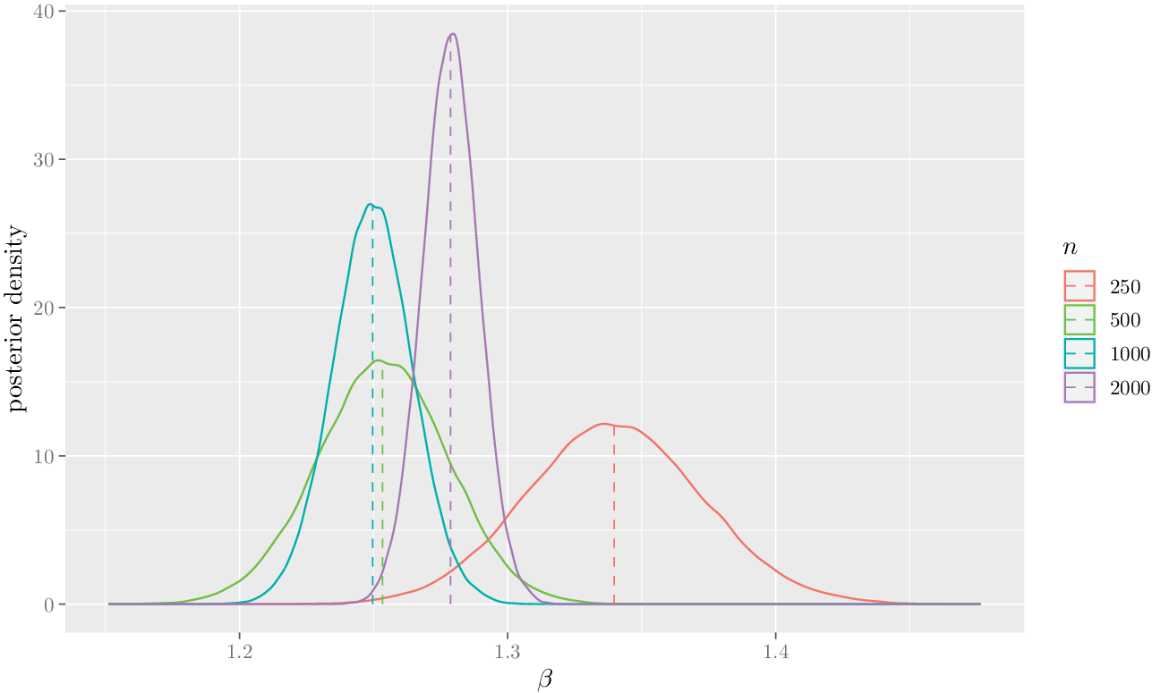
 for each sample size is computed from these MCMC sampled draws. Kernel smoothed versions of the posterior densities are given in Figure 1. As shown in Figure 1, as the sample size increases, the posterior density of
$\beta $
 under the base model concentrates on a value quite different from the true value of
$\beta $
 , indicating misspecification due to neglected endogeneity. In the extended (correctly specified) model, we have
Base model under neglected endogeneity: Marginal posterior densities of
$ \beta $
 for different sample sizes. Posterior mean is indicated by dashed vertical line.

Figure 1 Long description
The x-axis represents beta with values from 1.2 to 1.4. The y-axis represents posterior density with values from 0 to 40. Four bell-shaped curves are plotted, each with a dashed vertical line indicating its posterior mean.
* n equals 250 (red line): The shortest and widest curve, centered furthest to the right with a peak density of approximately 12 at beta equals 1.34.
* n equals 500 (green line): A slightly taller curve centered to the left of the red curve, with a peak density of approximately 16 at beta equals 1.25.
* n equals 1000 (teal line): A taller and narrower curve centered very close to the green curve, with a peak density of approximately 27 at beta equals 1.25.
* n equals 2000 (purple line): The tallest and narrowest curve, centered between the teal and red curves, with a peak density of approximately 38 at beta equals 1.28.
The legend on the right identifies the sample sizes n as 250, 500, 1000, and 2000, corresponding to the red, green, teal, and purple lines respectively.

The parameter of interest is now
$\psi := (\beta ,\gamma _{0},\gamma _{1},v)$
 . We use a default Student-t prior on v centered at the generalized method of moments (GMM) estimate and spread given by four times the GMM asymptotic variance. The prior of
$\theta $
 is the same as in the base model. The ETEL posterior for each of the four different sample sizes is sampled by the tailored one-block M–H method for 20,000 iterations beyond a burn-in of 1,000 cycles. The marginal posterior densities of
$\beta $
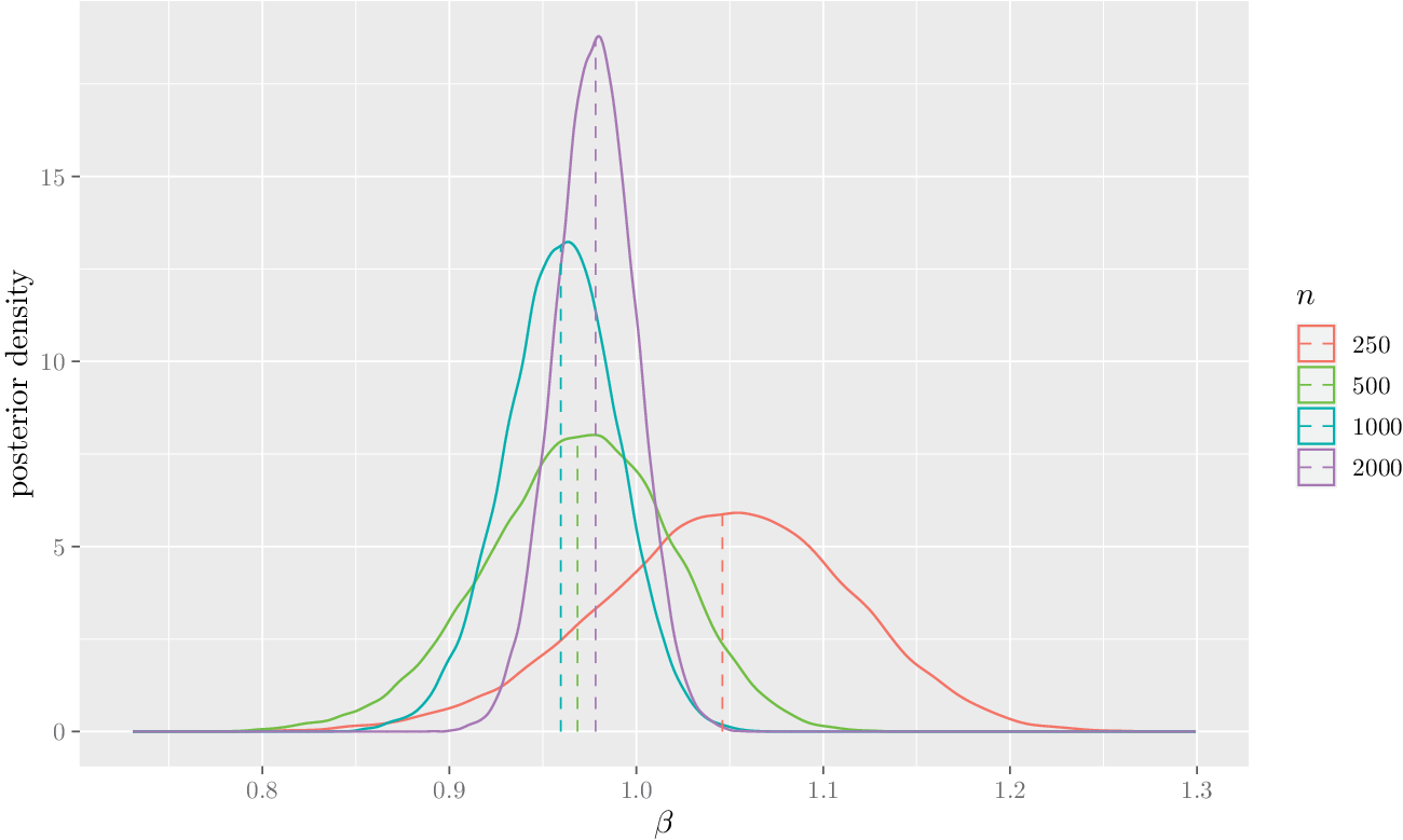
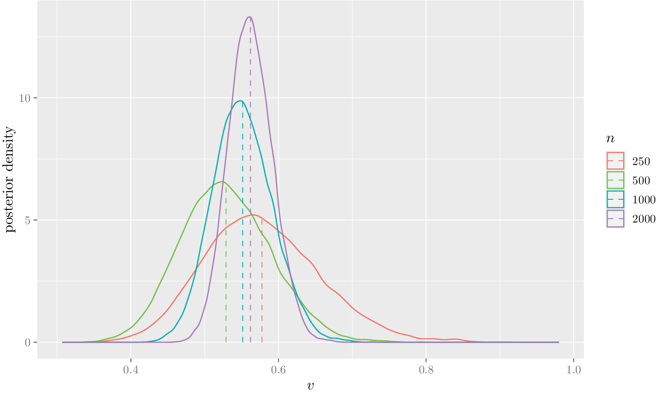
 are given in Figure 2 and those of v are in Figure 3. One can see that the posterior of
$\beta $
 , even for
$n=250$
 , is close to the true value of
$\beta $
 , and, for
$n=2,000$
 , is essentially centered around the true value. In addition, the posterior of v, the
$\text {cov}(x,\varepsilon )$
 , tends to concentrate around the true value of 0.6.
Extended model
($x_{i}$
 moment is inactive): Marginal posterior densities of
$ \beta $
 for different sample sizes. Posterior mean is indicated by dashed vertical line.

Figure 2 Long description
The X-axis represents beta, ranging from 0.8 to 1.3. The Y-axis represents posterior density, ranging from 0 to 15. Four bell-shaped curves are plotted, each with a dashed vertical line indicating its posterior mean.
* For n = 250 (red line), the curve is the widest and shortest, peaking at a density of approximately 6 near beta = 1.05.
* For n = 500 (green line), the curve is narrower and taller, peaking at a density of approximately 8 near beta = 0.97.
* For n = 1000 (teal line), the curve is significantly narrower and taller, peaking at a density of approximately 13 near beta = 0.96.
* For n = 2000 (purple line), the curve is the narrowest and tallest, peaking at a density of approximately 19 near beta = 0.98.
As the sample size n increases, the distribution of beta converges, indicated by the increasing height and decreasing width of the density peaks.
Extended model under neglected endogeneity: Marginal posterior densities of
$v = \text {cov}(x, \varepsilon )$
 for different sample sizes. Posterior mean is indicated by dashed vertical line.

Figure 3 Long description
The x-axis is labeled v and ranges from 0.4 to 1.0. The y-axis is labeled posterior density and ranges from 0 to over 10. Four bell-shaped curves are plotted, each with a corresponding dashed vertical line indicating its posterior mean.
* For n equals 250 (red line), the curve is the widest and shortest, peaking at a density of approximately 5 with a mean near 0.58.
* For n equals 500 (green line), the curve is slightly narrower and taller, peaking at a density of approximately 7 with a mean near 0.53.
* For n equals 1000 (teal line), the curve is significantly narrower, peaking at a density of approximately 10 with a mean near 0.55.
* For n equals 2000 (purple line), the curve is the narrowest and tallest, peaking at a density of approximately 14 with a mean near 0.56.
As the sample size n increases, the posterior density curves exhibit higher precision, characterized by a decrease in variance and an increase in peak height.
4 TESTING PROCEDURE
4.1 Bayes Factor
Our Bayesian test of endogeneity is given by the Bayes factor of model
$\mathcal {M}_{e}$
 versus model
$\mathcal {M}_{b}$
 defined as

where
$m(w_{1:n}|\mathcal {M}_{b}):=\int _{H_n} \widehat {q}(w_{1:n}|\theta ,\mathcal {M}_{b})\pi (\theta )d\theta $
 and
$m(w_{1:n}|\mathcal {M}_{e}) := \int _{H_n} \widehat {q}(w_{1:n}|\psi ,\mathcal {M}_{e})\pi (\psi )d\psi $
 are the model marginal likelihoods arising from the ETEL functions (also called marginal ETEL functions later on). We compute these by the method of Chib (Reference Chib1995), as extended to general M–H chains in Chib and Jeliazkov (Reference Chib and Jeliazkov2001). We select
$ \mathcal {M}_{e}$
 over
$\mathcal {M}_{b}$
 if
$\log ($
 BF
$_{eb})>0$
 and select
$ \mathcal {M}_{b}$
 otherwise.
According to the theory in Chib et al. (Reference Chib, Shin and Simoni2018), for valid comparisons of moment condition models, the competing models must arise from a common encompassing model and should have the same number of moment conditions. We have ensured that this condition is met by including the
$\mathbf {E} [\varepsilon _{i}(\theta )z_{2,i}]=0$
 restriction in the base model, and not excluding the
$\mathbf {E}[\varepsilon _{i}(\theta )x_{i}]=v$
 condition from the extended model.
Intuitively, the Bayes factor picks the correct model because
$\mathcal {M} _{b}$
 is correctly specified when x is exogenous and misspecified when x is endogenous; however,
$\mathcal {M}_{e}$
 is correctly specified in both cases. Therefore, from Chib et al. (Reference Chib, Shin and Simoni2018), it follows that
$\mathcal {M }_{b}$
 , which has
$(d-p)$
 overidentifying restrictions, rather than
$M_{e}$
 , which has
$(d-p-d_{x})$
 overidentifying restrictions, would be preferred by the Bayes factor when x is exogenous (because it has more overidentifying restrictions than
$\mathcal {M}_{e}$
 ), whereas
$\mathcal {M}_{e}$
 would be preferred when x is endogenous (because
$\mathcal {M}_{b}$
 in that case would be misspecified).
4.2 Rationale
In this section, we explain the rationale behind our testing procedure. The hypothesis that we want to test is the following:

against

Here, the subscripts
$miss$
 and
$cs$
 are for misspecification and correct specification, respectively. The previous hypothesis can equivalently be written as
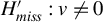
$H_{miss}': v\neq 0$
 and
$H_{cs}': v = 0$
 . Our approach based on
$\text {BF}_{eb}$
 is equivalent to a Bayes test for
$H_{miss}'$
 versus
$H_{cs}'$
 based on a mixture prior on v of the type
$\pi _0\delta _0(v) + (1 - \pi _0)\pi (v)$
 , where
$\delta _0(\cdot )$
 denotes a Dirac mass on zero,
$\pi _0\in [0,1]$
 , and
$\pi (\cdot )$
 is a continuous distribution. The two Bayes factors for these two approaches are numerically the same. The testing procedure works as follows: if
$\text {BF}_{eb}> 1$
 , we conclude that x is endogenous (that is, accept
$H_{miss}$
 ); if
$\text {BF}_{eb} < 1$
 , we conclude that x is exogenous (that is, accept
$H_{cs}$
 ). In the knife-edge case
$\text {BF}_{eb}=1$
 , the two models receive equal support from the data; for definiteness, we assign this tie to the base model.
The next theorem shows that
$H_{miss}$
 and
$H_{cs}$
 can be expressed in terms of KL divergences between P and the set
$\mathcal {Q}_{b}(\theta )$
 of distributions that satisfy the moment restriction that we want to test as well as additional moment restrictions that are known to hold for P.
Theorem 4.1. Suppose that there is a
$\theta \in \Theta $
 such that
$\mathbf {E}[\varepsilon _{i}(\theta )(z_{1,i}'z_{2,i}')']= 0$
 and that Assumption 1 holds true. Consider the following statements:
-
(i). P is such that $\nexists \theta \in \Theta $
such that
$\mathbf {E}[\varepsilon _{i}(\theta )x_{i}] = 0$
. -
(ii). $\mathrm {KL}(P||Q_b^*(\theta _*))>0$
. -
(iii). P is such that $\exists \theta \in \Theta $
such that
$\mathbf {E}[\varepsilon _{i}(\theta )x_{i}] = 0$
. -
(iv). $\mathrm {KL}(P||Q_b^*(\theta _*))=0$
.


Then, (i) is equivalent to (ii), and (iii) is equivalent to (iv).
This theorem makes clear that to test
$H_{miss}$
 and
$H_{cs}$
 one can equivalently focus on the KL divergence
$\mathrm {KL}(P||Q_b^*(\theta _*))$
 . Our Bayes test is based on Bayes factor and comparison of marginal likelihoods. There is a strict link between marginal likelihood and the KL divergence: log-marginal likelihood of the base model behaves asymptotically as
$- n \mathrm {KL}(P||Q_b^*(\theta _*))$
 plus a penalty term, where the penalty depends on the number of parameters to estimate, and similarly for the log-marginal likelihood of the extended model. We are going to demonstrate this fact in the rest of this section.
From the Chib (Reference Chib1995) identity, we have for the base model:
$\forall \theta \in H_n\subset \mathbb {R}^p$
 ,

and similarly for the extended model. Because this identity is true for every
$\theta \in H_n$
 , it is true for
$\theta = \theta _*$
 under Assumptions 1 and 3:
$\log m(w_{1:n}|\mathcal {M}_b) = \log \pi (\theta _*|\mathcal {M}_b) + \log \widehat {q}(w_{1:n}|\theta _*,\mathcal {M}_b) - \log \pi ^n(\theta _*|w_{1:n},\mathcal {M}_b)$
 . Next, let us introduce the local parameters
$h_{\theta }:=\sqrt {n}(\theta - \theta _*)$
 and
$h_{\psi }:=\sqrt {n}(\psi - \psi _\circ )$
 , so that by the formula for transformations of random variables:
$\pi ^n(\theta |w_{1:n},\mathcal {M}_b) = \pi _{h_{\theta }}^n(\sqrt {n}(\theta - \theta _{*})|w_{1:n},\mathcal {M}_b)n^{p/2}$
 and
$\pi ^n(\psi |w_{1:n},\mathcal {M}_e) = \pi _{h_{\psi }}^n(\sqrt {n}(\psi - \psi _{\circ })|w_{1:n},\mathcal {M}_e)n^{(p+d_x)/2}$
 , where
$\pi _{h_{\theta }}^n(\cdot |w_{1:n},\mathcal {M}_b)$
 and
$\pi _{h_{\psi }}^n(\cdot |w_{1:n},\mathcal {M}_e)$
 denote the posterior density of
$h_{\theta }$
 and
$h_{\psi }$
 , respectively. By replacing this in the expression of the marginal likelihoods, we obtain
$\forall \theta \in H_n\subset \mathbb {R}^p$
 ,

and,
$\forall \psi \in H_n\subset \mathbb {R}^{p+d_x}$
 ,

The intuition for expressing the posterior of
$\theta $
 in terms of the posterior of the local parameter is that the Jacobian of the transformation makes explicit the role played by the dimension of the model, while the local parameter has a posterior distribution that is approximately Gaussian. This is true in both cases (i) and (iii) of Theorem 4.1. Hence, the Jacobian induces an explicit dimension-dependent penalty through posterior concentration.
Therefore, the log-marginal likelihood decomposes into two terms that are bounded in probability as
$n\rightarrow \infty $
 (the prior ordinate evaluated at the pseudo-true value and the posterior ordinate of the local parameter) and two terms that diverge with n: the log-ETEL term and a model-dimension penalty of order
$\tfrac {1}{2}\log n$
 per parameter. Asymptotically, the marginal likelihood behaves like a penalized log-ETEL criterion, where the penalty arises endogenously from posterior concentration via the local reparameterization, rather than being imposed ad hoc.
Of course, for a testing procedure based on marginal likelihoods to be valid, it is necessary to establish that
$\pi _{h_{\theta }}^n(\sqrt {n}(\theta - \theta _{*}) \mid w_{1:n},\mathcal {M}_b)$
 and
$\pi _{h_{\psi }}^n(\sqrt {n}(\psi - \psi _{\circ }) \mid w_{1:n},\mathcal {M}_e)$
 are bounded in probability as
$n \rightarrow \infty $
 . This requirement can be quite challenging to verify, particularly in non-standard settings such as the one considered here, where there is no parametric likelihood and the models may be misspecified. We establish these results in Theorems D.6 and D.7 in the Supplementary Material, which refine Theorems 1 and 2 of Chib et al. (Reference Chib, Shin and Simoni2018).
A critical step in proving these results is to show that the log-ETEL function satisfies a stochastic local asymptotic normality (LAN) property. While the remainder of the Bernstein–von Mises argument follows standard lines, establishing stochastic LAN is challenging because the ETEL function is itself a random likelihood. In this article, we provide a new and more direct proof of the LAN property for the log-ETEL function (see Theorems D.1–D.3 in the Supplementary Material). Our proof leverages the specific structure of the IV regression problem: due to linearity, each term in the mean value theorem expansion of the log-ETEL function around
$\theta _*$
 can be controlled more directly and uniformly in
$h_{\theta }$
 over compact sets. This allows us to avoid the empirical process theory used in Chib et al. (Reference Chib, Shin and Simoni2018).
The final step toward understanding the asymptotic behavior of the marginal likelihood is provided by Theorems 4.2 and 4.3, which derive stochastic expansions of the log-ETEL function in the base and extended models. These expansions, which were not made explicit in Chib et al. (Reference Chib, Shin and Simoni2018), are new to the best of our knowledge.
Our starting point is the exact master identity for the log-ETEL, (2.12). Evaluating this identity at
$\theta =\theta _*$
 and writing
$\widehat \lambda (\theta _*)=\lambda _*(\theta _*)+ (\widehat \lambda (\theta _*)-\lambda _*(\theta _*))$
 , we obtain the expansion by performing a second-order Taylor expansion in
$\lambda $
 around
$\lambda _*(\theta _*)$
 . The stochastic LAN property delivers a linear representation for
$\sqrt {n}(\widehat \lambda (\theta _*)-\lambda _*(\theta _*))$
 , which, when substituted back into the master identity, yields the quadratic empirical-process terms reported below.
The assumptions under which the results hold are collected in Section 4.5. We use the notation
$\mathbf {E}_n[\cdot ] := n^{-1}\sum _{i=1}^n(\cdot )$
 for the empirical mean and
$\mathbb {G}_n f := \sqrt n(\mathbf {E}_n[f]-\mathbf {E}[f])$
 for the centered empirical process.
Theorem 4.2 (Base Model: Stochastic Expansion of Log-ETEL).
Let Assumptions 1–5 and 6 (d)–(f) hold. Then,

Moreover,

where
$\tau _i^{\dagger }(\lambda _*,\theta _*):=[dQ^*(\theta _*)/dP](w_i)$
 ,
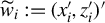
$\Omega _*^{\dagger }(\theta _*):= \mathbf {E}^{Q^*(\theta _*)}[\varepsilon _i(\theta _*)^2\widetilde w_i\widetilde w_i']$
 , and
$\widetilde {w}_i := (x_i',z_i')'$
 . In addition,

This theorem establishes a decomposition of the log-ETEL function for the base model
$\mathcal {M}_b$
 , characterizing its asymptotic behavior. This decomposition is used to prove the consistency of our Bayes factor testing procedure. Theorem 4.2 states that
$\log \widehat {q}(w_{1:n}|\theta _*,\mathcal {M}_{b}) + n\log n$
 can be expressed, up to an
$o_p(1)$
 term, as the sum of four random components. The third and fifth terms on the right-hand side of equation (4.3) are both of order
$\mathcal {O}_p(1)$
 , while the second and fourth terms are of order
$\mathcal {O}_p(n)$
 and
$\mathcal {O}_p(\sqrt {n})$
 , respectively, when
$x_i$
 is endogenous, and equal to zero when
$x_i$
 is exogenous. The fourth term is linear, with its rate
$\mathcal {O}_p(\sqrt {n})$
 following from the last part of the theorem, whereas the fifth term in (4.3) is quadratic. The term
$n\log n$
 does not affect the comparison, as it cancels out with the corresponding term in the log-ETEL function of the extended model, as shown in the next theorem.
For the extended model, we recall that
$\psi _\circ = (\theta _\circ ',v_\circ ')'$
 denotes the true value of the parameter in the extended model with
$v_{\circ } = \mathbf {E}[\varepsilon (\theta _\circ )x]$
 .
Theorem 4.3 (Extended Model).
Let Assumptions 2–4 with
$\Theta $
 replaced by
$\Psi $
 and Assumptions 5 and 6 (d)–(f) with
$\theta _*$
 and
$\lambda _*(\theta _*)$
 replaced with
$\theta _\circ $
 and
$0$
 , respectively, hold. Then,

where
$\Omega _{\psi _{\circ }} := \mathbf {E}[g_e(w_i,\psi _\circ )g_e(w_i,\psi _\circ )']$
 , and
$\mathbb {G}_n\left [g_e(w_i,\psi _\circ )'\right ] \Omega _{\psi _\circ }^{-1} \mathbb {G}_n\left [g_e(w_i,\psi _\circ )\right ]\xrightarrow {d}\chi _{d}^2$
 , where
$\chi _{d}^2$
 denotes a chi square distribution with d degrees of freedom.
Theorem 4.3 establishes the asymptotic behavior of the log-ETEL function of the extended model
$\mathcal {M}_e$
 . Unlike the base model,
$\log \widehat {q}(w_{1:n}|\psi _\circ ,\mathcal {M}_{e}) + n\log n$
 is equal, up to an asymptotically negligible term, to a quadratic random term that remains bounded in probability as
$n\rightarrow \infty $
 .
If
$\mathbf {E}[\varepsilon _i(\theta _\circ ) x_i] = 0$
 (exogenous case), so that the assumptions in Theorem 4.2 hold with
$\theta _*$
 replaced by
$\theta _\circ $
 and
$\lambda _*(\theta _*) = \lambda _*(\theta _\circ ) = 0$
 , then the log-ETEL function in the base model simplifies as

where
$\Omega _\circ := \mathbf {E}[\varepsilon _i(\theta _\circ )^2 \widetilde {w}_i\widetilde {w}_i']$
 ,
$\mathbb {G}_n\left [g_b(w_i,\theta _\circ )'\right ] \Omega _\circ ^{-1} \mathbb {G}_n\left [g_b(w_i,\theta _\circ )\right ]\xrightarrow {d}\chi _{d}^2$
 , and
$\chi _{d}^2$
 denotes a chi square distribution with d degrees of freedom. For the extended model, if
$\mathbf {E}[\varepsilon _i(\theta _\circ ) x_i] = 0$
 , then
$g_e(w_i,\psi _\circ ) = g_b(w_i,\theta _\circ )$
 and the log-ETEL function slightly simplifies as

where
$\mathbb {G}_n\left [g_b(w_i,\psi _\circ )'\right ] \Omega _{\psi _\circ }^{-1} \mathbb {G}_n\left [g_b(w_i,\psi _\circ )\right ]\xrightarrow {d}\chi _{d}^2$
 . Hence, when x is exogenous,
$\log \widehat {q}(w_{1:n}|\theta _\circ ,\mathcal {M}_{b}) $
 and
$\log \widehat {q}(w_{1:n}|\psi _\circ ,\mathcal {M}_{e})$
 are equal asymptotically and they cancel in the comparison of the marginal likelihoods.
In case of endogeneity, instead,
$\log \widehat {q}(w_{1:n}|\theta _\circ ,\mathcal {M}_{b}) $
 and
$\log \widehat {q}(w_{1:n}|\psi _\circ ,\mathcal {M}_{e})$
 are different and they play a central role in the comparison of marginal likelihoods. In this case, it is important to consider the behavior of the average log-ETEL function
$\frac {1}{n}\log \widehat {q}(w_{1:n}|\theta _*,\mathcal {M}_b)$
 which stays bounded asymptotically. The following two corollaries demonstrate that asymptotically the average log-ETEL functions behave as the KL divergence, up to a
$\log (n)$
 term. While these results are implicit in the definition of the ETEL, we provide here a formal and explicit statement and in the Appendix of their proof. This allows us to understand the behavior of the marginal likelihood.
Corollary 4.1 (Base Model).
Suppose Assumptions 1–5 and 6 (d)–(f) hold. Then, as
$n\rightarrow \infty $
 ,

where
$\mathbf {E}\left [\log (dQ_b^*(\theta _*)/dP)\right ] = \mathbf {E}\left [\log \Big (\frac {e^{\lambda _{*}(\theta _*)'g_b(w,\theta _*)}}{\mathbf {E}[e^{\lambda _*(\theta _*)'g_b(w,\theta _*)}]}\Big )\right ] = -\mathrm {KL}(P||Q_b^*(\theta _*))$
 .
Corollary 4.2 (Extended Model).
Suppose Assumptions 2–4 with
$\Theta $
 replaced by
$\Psi $
 , 5 and 6 (d)–(f) with
$\theta _*$
 and
$\lambda _*(\theta _*)$
 replaced with
$\theta _\circ $
 and
$0$
 , respectively, hold. Then, as
$n\rightarrow \infty $
 ,

where
$\mathbf {E}\left [\log (dQ_e^*(\psi _\circ )/dP)\right ] = \mathbf {E}\left [\log \Big (\frac {e^{\lambda _{*}(\psi _\circ )'g(w,\psi _\circ )}}{\mathbf {E}[e^{\lambda _*(\psi _\circ )'g(w,\psi _\circ )}]}\Big )\right ] = \mathrm {KL}(P||Q_e^*(\psi _\circ ))$
 .
Notice that
$\mathbf {E}\left [\log (dQ_e^*(\psi _\circ )/dP)\right ] = 0$
 since the extended model is correctly specified and so
$dQ_e^*(\psi _\circ )/dP = 1$
 .
From Theorems 4.2 and 4.3, and Theorems D.6 and D.7 in the Supplementary Material and from (4.1) and (4.2), there exists an N such that for every
$n>N$
 ,


These log-marginal likelihoods quantify the overall validity of the model. In fact, from these expressions, one sees that when
$x_i$
 is exogenous, that is,
$\mathbf {E}[\varepsilon _i(\theta _\circ ) x_i] = 0$
 , then
$\lambda _*(\theta _*) = 0$
 and
$\sum _{i=1}^n \log \left (\frac {e^{\lambda _*(\theta _*)'g_b(w_i,\theta _*)}}{\mathbf {E}_n[e^{\lambda _*(\theta _*)' g_b(w_j,\theta _*)}]}\right ) = 0$
 for every
$n\in \mathbb {N}$
 . Therefore, it is clear that asymptotically
$\log m(w_{1:n}|\mathcal {M}_b)$
 is larger than
$\log m(w_{1:n}|\mathcal {M}_e)$
 .
On the other hand, when there is no
$\theta \in \Theta $
 such that
$\mathbf {E}[\varepsilon _i(\theta ) x_i] = 0$
 , then
$\lambda _*(\theta _*) \neq 0$
 and
$\sum _{i=1}^n \log \left (\frac {e^{\lambda _*(\theta _*)'g_b(w_i,\theta _*)}}{\mathbf {E}_n[e^{\lambda _*(\theta _*)' g_b(w_j,\theta _*)}]}\right ) - n\log n$
 diverges to
$-\infty $
 faster than the last two terms in (4.9), so that asymptotically
$\log m(w_{1:n}|\mathcal {M}_b)$
 is smaller than
$\log m(w_{1:n}|\mathcal {M}_e)$
 . This is the main intuition of the consistency results in Theorems 4.4 and 4.5 in the next section. The proof of these theorems, which is provided in the Appendix, is more involved than this argument because the theorems provide an “if and only if” statement, which is stronger than consistency.
4.3 Consistency of the Testing Procedure
We now use the preceding theory to establish consistency of our testing procedure based on the Bayes factor constructed from the marginal ETEL functions. The theorems below establish that, as the sample size increases,
$BF_{eb}$
 selects
$\mathcal {M}_{b}$
 if and only if x is exogenous and selects
$\mathcal {M}_{e}$
 if and only if x is endogenous, with probability approaching 1.
Theorem 4.4. Let Assumptions 1–3, 5, 8, and 9 hold and let Assumptions 4 and 6 hold for
$\theta _*$
 and
$\lambda _*(\theta _*)$
 and also for
$\theta _*$
 and
$\lambda _*(\theta _*)$
 replaced with
$\theta _\circ $
 and
$0$
 , respectively. Let the priors on
$\theta $
 and
$\psi $
 be continuous probability measures that admit densities with respect to the Lebesgue measure and that are positive on a neighborhood of
$\theta _*$
 and
$\psi _{\circ }$
 , respectively. Let us consider the comparison of models
$\mathcal {M}_{b}$
 and
$\mathcal {M}_{e}$
 . Then,

if and only if there is no
$\theta \in \Theta $
 such that
$\mathbf {E}[\varepsilon _{i}(\theta )x_i]=0 $
 holds, and the limit is zero otherwise.
As we show in the proof, the failure of the necessary and sufficient condition
$\mathbf {E}[\varepsilon _{i}(\theta )x_{i}]=0$
 for any
$\theta \in \Theta $
 , is equivalent to the inequality
$\mathrm {KL}(P||Q_{e}^{\ast }(\psi ))<\mathrm {KL}(P||Q_{b}^{\ast }(\theta ))$
 , where
$\mathrm {KL}(P||Q_{e}^{\ast }(\psi _\circ )) = 0$
 . In this case, the log-ETEL function dominates the other components of the log-marginal ETEL function so that the built-in penalty does not play any role. Thus, as in the general result, in (Chib et al., Reference Chib, Shin and Simoni2018, Thm. 3.2) for moment condition models, comparing the log-marginal likelihoods of the base and extended models, and selecting the one with the higher value, in the limit, selects the model that is closest in the KL divergence to the true model. In the framework of the present paper, this means that the comparison of marginal likelihoods allows to correctly conclude that
$x_i$
 is endogenous.
Next, we show what happens when the variables
$x_i$
 are exogenous so that the moment restriction
$\mathbf {E}[\varepsilon _{i}(\theta )x_{i}]=0$
 holds for a particular value
$\theta _\circ $
 and the two models under comparison are correctly specified. The next theorem states that in this case the base model is selected. This is understandable through an argument of parsimony: the base model has the smaller number of parameters to estimate and so it is the preferred one when it is correctly specified.
Theorem 4.5. Let Assumptions 1–3, 5, 8, and 9 hold and let Assumptions 4 and 6 hold for both
$\theta _*$
 and
$\lambda _*(\theta _*)$
 and also for
$\theta _*$
 and
$\lambda _*(\theta _*)$
 replaced with
$\theta _\circ $
 and
$0$
 , respectively. Let the priors on
$\theta $
 and
$\psi $
 be continuous probability measures that admit densities with respect to the Lebesgue measure and that are positive in a neighborhood of
$\theta _*$
 and
$\psi _{\circ }$
 , respectively. Let us consider the comparison of models
$\mathcal {M}_{b}$
 and
$\mathcal {M}_{e}$
 . Then,

if and only if there is a
$\theta _\circ \in \Theta $
 such that
$\mathbf {E}[\varepsilon _{i}(\theta _\circ )x_i]=0 $
 holds.
When x is exogenous, as in the previous theorem, both the log-ETEL function and the built-in penalty play a role in selecting the correct model.
Discussion. In this and the previous section, we demonstrate that our model selection criteria favor a model with a smaller KL information criterion (KLIC). When two models share the same KLIC, our procedure opts for the model with a greater number of overidentifying restrictions, that is, a more parsimonious or less flexible model. Interestingly, this aligns with the goal of Sin and White (Reference Sin and White1996)’s penalized likelihood criteria for a parametric model. Consequently, our proposed model selection procedure in this article and Chib et al. (Reference Chib, Shin and Simoni2018) can be viewed as a fully Bayesian semi-parametric version of consistent model selection criteria, applied specifically to an endogeneity testing problem. Unlike other frequentist procedures, the “penalty” term required for consistency is inherently built into our Bayesian calculation. This point was not stressed in Chib et al. (Reference Chib, Shin and Simoni2018) and it is a contribution of this article.
Andrews (Reference Andrews1999), Andrews and Lu (Reference Andrews and Lu2001), and Hong, Preston, and Shum (Reference Hong, Preston and Shum2003) have proposed and studied model selection criteria for moment condition models, even though a formal likelihood function is not defined. These criteria involve a penalization term that is attached to the GMM and, more broadly, the generalized empirical likelihood (GEL) objective function, rather than the likelihood function. Examples of such frequentist model selection approaches based on GMM estimation can be found in Section A of the Supplementary Material. However, the relationship between these model selection criteria and the KLIC minimization principle of Sin and White (Reference Sin and White1996) for potentially misspecified parametric models is not immediately apparent.
It is noteworthy that our procedure exhibits the same asymptotic behavior as Hong and Preston (Reference Hong and Preston2012)’s GEL Bayes factor. They impose a separate prior on the Lagrangian multiplier that is independent of
$\theta $
 , which does not guarantee the imposition of moment restrictions. In contrast, we introduce an additional parameter v to the “inactive” moment restriction, ensuring that our prior on
$\theta $
 and v respects the moment restrictions.
4.4 Testing among More Than Two Models
Our testing procedure can be extended to settings in which more than two models are compared. Consider the case in which only a subset of the variables in x is endogenous. To start, suppose that
$d_x = 2$
 and that only
$x_1$
 is endogenous, whereas
$x_2$
 is exogenous. That is,
$\mathbf {E}[\varepsilon (\theta _{\circ })(x_2,z_1')']=0$
 , while there exists no
$\theta \in \mathbb {R}^p$
 such that
$\mathbf {E}[\varepsilon (\theta )x_1]=0$
 . If we compare only the base and extended models,
$\mathcal {M}_b$
 and
$\mathcal {M}_e$
 , we could erroneously conclude that
$x_1$
 and
$x_2$
 are both endogenous. Instead, it is more appropriate to consider the following models:
$\mathcal {M}_b$
 ,
$\mathcal {M}_e$
 ,
$\mathcal {M}_{e_1}$
 , and
$\mathcal {M}_{e_2}$
 , where, for
$i=1,2$
 ,
$\mathcal {M}_{e_i}$
 is the model defined by the moment condition

where

$\psi _i :=(\theta ,v^{(i)})\in \Psi $
 ,
$\Psi :=\Theta \times \mathcal {V}$
 ,
$\mathcal {V}\subset \mathbb {R}^{2}$
 with
$v^{(i)} = (v_1^{(i)}, v_2^{(i)})$
 and
$v_j^{(i)}\in \mathbb {R}$
 for
$j=1,2$
 , and
$\mathcal {Q}_{e_i}(\psi _i) := \left \{Q\in \mathbb {M};\,\mathbf {E}^{Q}[g_{e_i}(w,\psi _i)] = 0\right \} $
 . We enforce the restriction that one component of x is treated as exogenous by setting the corresponding element of
$v^{(i)}$
 to zero. Specifically, define
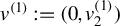
$v^{(1)} := (0,v_{2}^{(1)})$
 and
$v^{(2)} := (v_{1}^{(2)},0)$
 . Model
$\mathcal {M}_{e_{1}}$
 treats
$x_{1}$
 as exogenous and allows
$x_2$
 to be endogenous, while model
$\mathcal {M}_{e_{2}}$
 treats
$x_{2}$
 as exogenous and allows
$x_1$
 to be endogenous.
This construction allows a direct application of our baseline-versus-extended comparison. Treat
$\mathcal {M}_e$
 as the common reference extended model and compare
$\mathcal {M}_{e_i}$
 against
$\mathcal {M}_e$
 . If the marginal likelihood of
$\mathcal {M}_{e_2}$
 exceeds that of
$\mathcal {M}_e$
 , then the data support the restriction
$v_2=0$
 , suggesting that
$x_2$
 is exogenous while
$x_1$
 is treated as endogenous. Similarly, if the marginal likelihood of
$\mathcal {M}_{e_1}$
 exceeds that of
$\mathcal {M}_e$
 , then the data support
$v_1=0$
 , suggesting that
$x_1$
 is exogenous while
$x_2$
 is treated as endogenous.
More generally, when more than two models are under consideration, one can compare them via their marginal likelihoods. In our context, these candidate models are obtained from the extended model by setting a subset of the elements of v to zero. In total, there are
$2^{d_x}$
 models, including the base and extended models. Each model corresponds to a configuration of which elements of x are treated as endogenous:
$x_i$
 is treated as endogenous when the associated
$v_i$
 is unrestricted, whereas
$v_i=0$
 corresponds to
$x_i$
 being treated as exogenous. Marginal-likelihood comparison over this finite model set selects the configuration most supported by the data.
Moreover, our endogeneity testing can be enriched by comparing different model specifications. For example, suppose x is scalar and consider linear versus quadratic specifications,

Then endogeneity of
$x_i$
 can be assessed under each specification, leading to four candidate models, linear-exogenous, linear-endogenous, quadratic-exogenous, and quadratic-endogenous. A marginal likelihood comparison can be used to select the best model among these candidates. We apply this idea in our real data example (BLP model). In that setting, we consider four candidate models that jointly vary the functional form and the endogeneity status of price, namely, linear-exogenous, linear-endogenous, nonlinear-exogenous, and nonlinear-endogenous. Marginal likelihood comparison over these four candidates simultaneously assesses endogeneity within each specification and delivers a unified ranking across specifications.
Section B of the Supplementary Material reports Monte Carlo experiments for these two use cases (see Sections B.1 and B.2 of the Supplementary Material).
4.5 Assumptions
We provide the assumptions that we use to prove the results in the previous sections. The first assumption ensures that the set of distributions satisfying the moment conditions is non-empty, which is necessary for the ETEL to be well defined. It guarantees that the dual representation of the optimization problem (2.5) holds even when
$P\notin \mathcal {Q}_{b,\theta }$
 for every
$\theta \in \Theta $
 . In fact, in the latter case, it is possible that
$Q_b^*(\theta )$
 and P do not have a common support for any
$\theta $
 , in which case, the equality in (2.7) does not hold (see Sueishi (Reference Sueishi2013) for a discussion on this point).
Assumption 1 (Non-Emptiness).
When
$\mathbf {E}[\varepsilon _{i}(\theta )x_{i}]\neq 0$
 for every
$\theta \in \Theta $
 , there exists
$Q\in \bigcup _{\theta \in \Theta }\mathcal {Q}_{b,\theta }$
 such that Q is mutually absolutely continuous with respect to P, where
$\mathcal {Q}_{b,\theta }$
 is defined in (3.3).
This assumption implies that there is a
$\theta $
 for which
$\mathcal {Q}_{b,\theta }$
 is non-empty, that
$dQ_b^{*}(\theta )/dP = \Big (\frac {e^{\lambda _{*}(\theta )'g(w,\theta )}}{\mathbf {E}[e^{\lambda _*(\theta )'g(w,\theta )}]}\Big )$
 and that
$\theta _{\ast }$
 is identified by (3.4). In addition, by assuming mutual absolute continuity, it ensures that both
$\mathrm {KL}(Q_b^{*}(\theta )||P)$
 and
$\mathrm {KL}(P||Q_b^{*}(\theta ))$
 are well defined. We then assume that
$\theta _*$
 is unique.
Assumption 2 (Identification).
The maximizer
$\theta _*$
 defined as the minimizer of
$\mathrm {KL}(P||Q^*(\theta ))$
 with respect to
$\theta \in \Theta $
 is unique and is in the interior of
$\Theta $
 , where the interior is defined with respect to the topology in
$\mathbb {R}^p$
 .
Since under Assumption 1,
$\theta _*$
 coincides with the minimizer in (3.4), then the previous assumption implies uniqueness also of the latter.
As we have pointed out in Section 2, the ETEL is not defined at the
$\theta $
 s for which the optimization problem (2.5) does not have a feasible solution, that is, at the
$\theta $
 s that do not belong to the set
$H_n$
 in (2.6). Assumption 1 guarantees that asymptotically the optimization problem (2.5) is feasible at
$\theta _*$
 . Similarly, if the model is correctly specified, then the optimization problem (2.5) is feasible at
$\theta _{\circ }$
 (or
$\psi _{\circ }$
 depending on which model we consider). However, this is not enough for our asymptotic analysis. Instead, we need to assume that (2.5) has a solution for every
$\theta $
 that is sufficiently close to
$\theta _*$
 with probability approaching
$1$
 . The required notion of how close is specified in the next assumption, for which we introduce the following ball. For any sequence
$M_n\rightarrow \infty $
 as
$n\rightarrow \infty $
 , and any
$\widetilde \theta \in \Theta $
 , define the
$n^{-1/2}$
 -ball around
$\widetilde \theta $
 as
$B(\widetilde \theta ,M_n n^{-1/2}) := \{\theta \in \Theta :\,\|\theta - \widetilde \theta \| \leq M_n n^{-1/2}\}.$
 The ball
$B(\widetilde \theta ,M_n n^{-1/2})$
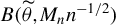 shrinks to
$0$
 slightly slower than
$n^{-1/2}$
 depending on how fast
$M_n$
 goes to
$\infty $
 . The
$n^{-1/2}$
 -ball
$B(\widetilde \psi ,M_n n^{-1/2})$
 around some
$\widetilde \psi \in \Psi $
 is defined similarly. In addition, denote by
$int \Delta _n := \{q := (q_1,\ldots ,q_n)'; \sum _{i=1}^n q_i = 1, \; q_1>0,\ldots ,q_n>0\}$
 the interior of the
$n-1$
 simplex. Finally, for any sequence
$M_n\rightarrow \infty $
 :
$B_{*,n} := \bigcap _{\{M_n; M_n\rightarrow \infty \} }B(\theta _*, M_n n^{-1/2})$
 and
$B_{\circ ,n} := \bigcap _{\{M_n; M_n\rightarrow \infty \} }B(\psi _{\circ },M_n n^{-1/2})$
 .
Assumption 3. As
$n\rightarrow \infty $
 , for every
$\theta \in B_{*,n}$
 ,

and
$\mathbf {E}^{Q_*}[g_b(w,\theta )]=0$
 . Similarly, as
$n\rightarrow \infty $
 and for every
$\psi \in B_{\circ ,n}$
 ,

and
$\mathbf {E}[g_e(w,\psi )]=0$
 .
This assumption is much weaker than requiring that (2.5) has a solution for every
$\theta \in \Theta $
 with probability approaching
$1$
 . Even if not explicitly stated in the literature, a similar assumption is necessary for the frequentist ETEL, EL, and ET estimators.
The next four assumptions concern the model. Compared to the assumptions in Chib et al. (Reference Chib, Shin and Simoni2018), our assumptions are weaker due to the linearity in
$\theta $
 of the moment functions
$g_b(w,\theta )$
 and
$g_e(w,\theta )$
 . Consequently, assumptions regarding the continuity of the moment functions and their derivatives are automatically satisfied. Recall the notation
$w_i:= (y_i, x_i', z_i')'$
 ,
$z_i := (z_{1,i}',z_{2,i}')'$
 and
$\tilde w_{1,i} := (x_i', z_{1,i}')'$
 . Moreover, we denote
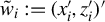
$\tilde w_i := (x_i', z_i')'$
 ,
$\|\cdot \|_2$
 the Euclidean norm and
$\|\cdot \|_{op}$
 the operator norm.
Assumption 4. (a)
$w_i$
 ,
$i=1,\ldots , n$
 are i.i.d. observable random variables with each one taking values in a complete probability space
$(\mathcal {W},\mathfrak {B}_{\mathcal {W}},P)$
 , where
$\mathcal {W}\subseteq \mathbb {R}^{d + 1}$
 ,
$\mathfrak {B}_{\mathcal {W}}$
 is the associated
$\sigma $
 -field, and P is a probability distribution satisfying model (3.1); (b)
$\Theta \subset \mathbb {R}^p$
 is compact and connected; (c) for every
$\lambda $
 in a neighborhood of
$\lambda _*(\theta _*)$
 , the matrix
$\mathbf {E}[e^{\lambda '\widetilde w_{i} \varepsilon _i(\theta _*)}\varepsilon _i(\theta _*)^2\widetilde w_i \widetilde w_i']$
 has the smallest (resp. largest) eigenvalue bounded away from zero (resp. infinity).
Assumption 5. (a)
$\mathbf {E}[\tilde w_i \tilde w_{1,i}']<\infty $
 with rank p.
Assumptions 4 and 5 are standard in the literature (see, e.g., Schennach Reference Schennach2007). The following assumption instead is new and it is used to prove the approximation for the marginal likelihood. We denote by
$\widetilde {w}_{i,k}$
 the kth component of
$\widetilde {w}_i$
 . Moreover, for any
$\delta>0$
 and for some constant
$C>0$
 , we denote by
$B_{\delta }(\lambda _*) := \{\lambda \in \mathbb {R}^d; \|\lambda - \lambda _*(\theta _*)\|_2 \leq C\delta \}$
 (resp.
$B_{\delta }(\theta _*) := \{\theta \in \mathbb {R}^p; \|\theta - \theta _*\|_2 \leq C\delta \}$
 ) a closed ball in
$\mathbb {R}^d$
 (resp. in
$\mathbb {R}^p$
 ) centered around
$\lambda _* := \lambda _*(\theta _*)$
 (resp.
$\theta _*$
 ) with radius
$\delta $
 , where
$\|\cdot \|_2$
 denotes the Euclidean norm. For any
$\delta>0$
 ,
$q\in \mathbb {N}_+$
 , a set B, and a function
$\gamma :\mathbb {R}^{d+1}\times \mathbb {R}^p\rightarrow \mathbb {R}$
 , we introduce the following set of functions:
$\mathcal {F}_{q,\delta }(B;\gamma ) := \{f:B\times \mathbb {R}^{d+1}\times B_{\delta }(\theta _*) \rightarrow \mathbb {R}^q; \|g(u,v,\theta )\|_2 \leq \gamma (v,\theta ),\, \forall u\in B\}$
 . For a random vector w, we denote with
$w_k$
 its kth component. Finally,
$K_n\subset \mathbb {R}^p$
 denotes a compact set centered on
$0$
 .
Assumption 6. For any
$\delta> 0$
 , there exist real-valued functions
$\gamma _j(w,\theta )$
 ,
$j=0,1,2,3,4,5$
 , defined on
$\mathbb {R}^{d+1}\times B_{\delta }(\theta _*) $
 and such that
$\mathbf {E}[\gamma _j(w,\theta )] < \infty $
 , for
$j=0,1,2,3,4,5$
 and
$\forall \theta \in B_{\delta }(\theta _*)$
 , and such that:
-
(a) the function $(\lambda ,w,\theta )\mapsto e^{\lambda '\widetilde w \varepsilon (\theta )} \widetilde w \varepsilon (\theta )\in \mathcal {F}_{d,\delta }(B_{\delta }(\lambda _*);\gamma _0)$
; -
(b) the function $(\lambda ,w,\theta )\mapsto e^{\lambda ' \widetilde w \varepsilon _i(\theta )} \in \mathcal {F}_{1,\delta }(B_{\delta }(\lambda _*);\gamma _1)$
; -
(c) the function $((\lambda ',h')',w,\theta )\mapsto e^{\lambda '\widetilde w \varepsilon (\theta _*)} \varepsilon (\theta )^{j - 1}\widetilde {w}_{k}^{\ell }(h'\widetilde {w}_{1})^{\ell '} \widetilde {w}_{k}^{\ell "} \in \mathcal {F}_{1,\delta }(B_{\delta }(\lambda _*)\times K_n;\gamma _2)$
for either
$(j,\ell ,\ell ',\ell ")=(1,1,1,0)$
, or
$(j,\ell ,\ell ',\ell ")=(1,2,2,0)$
, or
$(j,\ell ,\ell ',\ell ")=(2,1,1,1)$
; -
(d) the function $(\lambda ,w,\theta ) \mapsto e^{2\lambda '\widetilde w \varepsilon (\theta _*)}\varepsilon (\theta _*)^2 \left \|\widetilde w \right \|_2^2 \in \mathcal {F}_{1,\delta }(B_{\delta }(\lambda _*);\gamma _3)$
; -
(e) the function $(\lambda ,w,\theta )\mapsto e^{\ell \lambda 'g(w,\theta )}\widetilde w_{j} \widetilde w_{k}\varepsilon (\theta )^{\ell '} \widetilde w_{k'}^{i} \in \mathcal {F}_{1,\delta }(B_{\delta }(\lambda _*);\gamma _4)$
for every
$j,k,k'=1,\ldots ,d$
, and for either
$(\ell ,\ell ',i)=(1,1,1)$
, or
$(\ell ,\ell ',i)=(1,2,0)$
, or
$(\ell ,\ell ',i)=(1,3,1)$
, or
$(\ell ,\ell ',i)=(2,4,2)$
, and where
$\gamma _4$
may depend on all the previous indices; -
(f) the function $((\lambda ',h')',w,\theta )\mapsto e^{\lambda '\widetilde w \varepsilon (\theta _*)} \varepsilon (\theta )\widetilde {w}\,\lambda '\widetilde {w}\,h'\widetilde {w}_{1}\in \mathcal {F}_{d,\delta }(B_{\delta }(\lambda _*)\times K_n;\gamma _5)$
; -
(g) the function $((\lambda ',h')',w,\theta )\mapsto e^{\lambda '\widetilde w \varepsilon (\theta _*)} \varepsilon (\theta )^j\widetilde {w}\,\lambda '\widetilde {w}\,(h'\widetilde {w}_{1})^{\ell } \widetilde {w}_k\in \mathcal {F}_{d,\delta }(B_{\delta }(\lambda _*)\times K_n;\gamma _6)$
for every
$k=1,\ldots ,d$
, and for either
$(j,\ell )=(2,1)$
, or
$(j,\ell )=(1,2)$
.
















This regularity assumption is a weak moment condition, requiring the existence of an upper bound—dependent on the data and on
$\theta $
 —with finite expectation for every
$\theta \in B_{\delta }(\theta _*)$
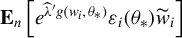
 . This condition ensures that a uniform Law of Large Number holds (see, e.g., (Newey and McFadden, Reference Newey and McFadden1994, Lemma 2.4)). In particular, we use this assumption in our proofs to establish the uniform convergence in probability of several terms, including:
$\mathbf {E}_n\left [e^{\widehat \lambda 'g(w_i,\theta _*)}\varepsilon _i(\theta _*)\widetilde {w}_{i}\right ]$
 ,
$\mathbf {E}_n\left [e^{\widehat \lambda 'g(w_i,\theta _*)}\widetilde {w}_{1,i}\widetilde {w}_{i}\right ]$
 ,
$h'\mathbf {E}_n\left [e^{\widehat \lambda 'g(w_i,\theta _*)} h'\widetilde {w}_{1,i}\widetilde {w}_{i}'\widehat \lambda \varepsilon _i(\theta _*)\widetilde {w}_i\right ]$
 , and
$\mathbf {E}_n\left [e^{\widehat \lambda 'g(w_i,\theta _*)}\varepsilon _i(\theta _*)\widetilde {w}_{1,i}\widetilde {w}_{i}\right ]$
 . The uniform convergence must hold uniformly over
$\widehat \lambda $
 in a closed ball
$B_{\delta }(\lambda _*(\theta _*))$
 . Additionally, this assumption also guarantees that the dominance condition required for the application of the dominated convergence theorem is satisfied, which is another result used in the proofs.
Part (e) of the previous assumption implies that

is bounded away from infinity for every
$k'\in \{1,\ldots ,d\}$
 which is what we need in the proof because this operator norm is upper bounded by
$d\,\max _{j,k\in \{1,\ldots ,d\}}|e^{\ell \lambda 'g(w,\theta _*)}\widetilde w_{j} \widetilde w_{k}\varepsilon (\theta _*)^{\ell } \widetilde w_{k'}^{i} |$
 for every
$k'\in \{1,\ldots , d\}$
 .
An assumption similar to Assumption 6 is necessary to establish uniform convergences of
$\mathbf {E}_n\left [\varepsilon _i(\theta )\widetilde {w}_{i}\right ]$
 and
$\mathbf {E}_n\left [\varepsilon _i(\theta )\widetilde {w}_{i} \widetilde {w_i}\right ]$
 uniformly over
$\theta \in B_{\delta }(\theta _*)$
 . For this, we introduce the following proposition.
Assumption 7. For any
$\delta> 0$
 , there exist real-valued functions
$\gamma _{\circ ,j}(w)$
 ,
$j=1,2$
 , defined on
$\mathbb {R}^{d+1}$
 and such that
$\mathbf {E}[\gamma _j(w)] < \infty $
 , for
$j=1,2$
 and:
-
(a) $\|\widetilde w \varepsilon (\theta )\| \leq \gamma _{\circ ,1}$
for every
$\theta \in B_{\delta }(\theta _*)$
; -
(b) $|\varepsilon (\theta )\widetilde w_j \widetilde w_k | \leq \gamma _{\circ ,2}$
for every
$\theta \in B_{\delta }(\theta _*)$
; -
(c) $\|h'\widetilde {w}_{1} \widetilde {w}'\| \leq \gamma _{\circ ,3}$
for every
$h\in K_n$
.





For the next assumption, we denote by
$\Theta _{n}:=\{\Vert \theta -\theta _{\ast }\Vert \leq M_{n}/\sqrt {n}\}$
 a ball around
$\theta _{*}$
 with the radius at most
$M_{n}/\sqrt {n}$
 , where
$M_{n}$
 is any sequence of positive constants diverging to
$+\infty $
 . We denote by
$\ell _{n,\theta }(w_i)$
 the log-likelihood function for one observation
$w_i$
 :
$\ell _{n,\theta }(w_i) := \log \widehat {q}_i(\theta |\mathcal {M}_b)$
 , and by
$\ell _{n,\theta }(w_{1:n}) := \sum _{i=1}^n \ell _{n,\theta }(w_i) = \log \widehat {q}(w_{1:n}|\theta ,\mathcal {M}_b)$
 the log-ETEL function. We recall that both
$\ell _{n,\theta }(w_i)$
 and
$\ell _{n,\theta }(w_{1:n})$
 are defined only for
$\theta \in H_n$
 and that under Assumption 3 they are at least defined on
$B_{*,n}$
 . The next assumption controls the behavior of the ETEL function
$\theta \mapsto \ell _{n,\theta }(w_{i})$
 at a distance from
$\theta _*$
 and it ensures that
$\theta _*$
 is well-separated from the
$\theta $
 s that are at a certain distance from it.
Assumption 8 (Base Model).
Assume that there exists a constant
$C>0$
 such that

where
$M_n$
 is the same sequence used to define
$\Theta _n$
 .
A condition similar to Assumption 8 is in (Kleijn and Van der Vaart, Reference Kleijn and Van der Vaart2012, Lemma 4.2) and it is also related to the classical condition in, for example, (Lehmann and Casella, Reference Lehmann and Casella1998, Assump. 6.B.3) and (Chernozhukov and Hong, Reference Chernozhukov and Hong2003, Assump. 3). However, in our case, the supremum in the assumption is taken over a smaller set, which is
$H_n\cap \Theta _n^c$
 , instead of over
$\Theta _n^c$
 as in the mentioned literature. To better understand the meaning of this assumption, note that asymptotically the log-ETEL function is maximized at the pseudo-true value
$\theta _*$
 . Hence, Assumption (4.14) requires that if the parameter
$\theta $
 is far from the pseudo-true value
$\theta _{*}$
 , that is
$\|\theta -\theta _* \|> M_{n}/\sqrt {n}$
 , then the sum
$\sum _{i=1}^{n} \ell _{n,\theta }(w_{i})$
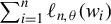 evaluated at such a
$\theta $
 must be small relative to the sum
$\sum _{i=1}^{n}\ell _{n,\theta _*}(w_{i})$
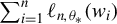 , which is the maximum value. Controlling this behavior is important because the posterior involves integration over the whole support of
$\theta $
 . Subsets of
$\Theta $
 that can be distinguished from
$\theta _*$
 uniformly (with probability approaching
$1$
 as
$n\rightarrow \infty $
 ) based on the ETEL function will receive a posterior probability that is asymptotically negligible. An alternative to this condition would be to require the existence of asymptotically consistent tests
$\phi _n$
 that are able to distinguish from the true distribution P in a uniform way, that is, for every
$\epsilon>0$
 , there exists a sequence of tests
$\{\phi _n\}$
 such that as
$n\rightarrow $
 0,

Similarly, for the extended model, we denote by
$\ell _{n,\psi }(w_i)$
 the log-likelihood function for one observation
$w_i$
 :
$\ell _{n,\psi }(w_i) := \log \widehat {q}_i(\psi |\mathcal {M}_e)$
 and by
$\ell _{n,\psi }(w_{1:n}) := \sum _{i=1}^n \ell _{n,\psi }(w_i) = \log \widehat {q}(w_{1:n}|\psi ,\mathcal {M}_e)$
 the log-ETEL function. The next assumption has the same interpretation of Assumption 8 but for the extended model.
Assumption 9 (Extended Model).
Assume that there exists a constant
$C>0$
 such that as
$n\rightarrow \infty $
 ,

where
$M_n$
 is any sequence of positive constants diverging to infinity.
4.6 Experiments
Consider the same generating process as in Section 3.4, and suppose that
$(\varepsilon _{i},u_{i},v_{i})$
 have a joint distribution induced by a Gaussian copula with covariance matrix
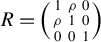 . The parameter
$\rho $
 controls the degree of endogeneity. We let
$\rho $
 take values in the set from
$-0.5$
 to 0.5, in increments of 0.1. For each value of
$\rho $
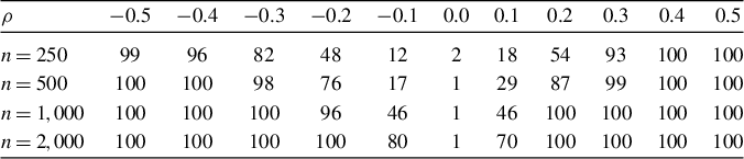
 in this set, we generate 100 samples of size n. For each sample, we compute the base and extended models and calculate the log-marginal likelihoods. We then count the number of times the log-marginal likelihood of
$\mathcal {M}_{e}$
 exceeds that of
$\mathcal {M}_{b}$
 . The results are given in Table 1. We can see from this table that even for small values of
$\rho $
 , our test of endogeneity correctly concludes that the correct model is
$\mathcal {M}_{e} $
 .
Model selection frequencies

Table 1 Long description
The table consists of 12 columns and 5 rows.
Header Row: The first column is labeled rho. Subsequent columns are labeled with rho values: minus 0.5, minus 0.4, minus 0.3, minus 0.2, minus 0.1, 0.0, 0.1, 0.2, 0.3, 0.4, and 0.5.
Row 2 (n = 250): Values are 99, 96, 82, 48, 12, 2, 18, 54, 93, 100, 100.
Row 3 (n = 500): Values are 100, 100, 98, 76, 17, 1, 29, 87, 99, 100, 100.
Row 4 (n = 1,000): Values are 100, 100, 100, 96, 46, 1, 46, 100, 100, 100, 100.
Row 5 (n = 2,000): Values are 100, 100, 100, 100, 80, 1, 70, 100, 100, 100, 100.
The data shows that as the absolute value of rho increases or the sample size n increases, the frequency of selecting model M sub e over model M sub b approaches 100. The lowest selection frequencies occur when rho is 0.0.
Note: Results are from 100 replications of data simulated from the design in Example 1. For each combination of n and
$\mathrm {Cov}(\varepsilon ,u)=\rho $
 , the entries give the number of times in 100 replications of the data that the log-marginal likelihood of
$\mathcal {M}_{e}$
 exceeds the log-marginal likelihood of
$\mathcal {M}_{b}$
 .
5 REAL DATA EXAMPLES
5.1 Causal Effect of Price on Automobile Demand
We consider the classic problem of automobile demand studied in Berry, Levinsohn, and Pakes (Reference Berry, Levinsohn and Pakes1995). This problem has recently been revisited by Chernozhukov, Hansen, and Spindler (Reference Chernozhukov, Hansen and Spindler2015), henceforth, BLP and CHS, respectively. Apart from its intrinsic value, this problem is worth analyzing because it involves a realistically large number of controls and instruments.
To set up the problem, let
$y_{ijt}$
 denote the log of the ratio of the market share of product i in market j at time t, relative to an external option, and let
$x_{ijt}$
 denote the potentially endogenous automobile price variable. In the sample data, this variable is demeaned. For controls, let
$z_{ijt}$
 denote the observed characteristics of the product. In BLP, these are taken to be a constant, an air conditioning dummy (
$air$
 ), horsepower divided by weight (
$hpwt$
 ), miles per dollar (
$mpd$
 ), and vehicle size (
$space$
 ). In our notation,
$y_{ijt} = x_{ijt} \, \beta + {z}_{1ijt}^{\prime }{\gamma }+ \varepsilon _{i}$
 , where
${z}_{1ijt}=(1, mpd_{ijt}, space:{ijt}, hpwt_{ijt}, air_{ijt})$
 . BLP used 10 instruments, 5 formed by summing the value of these 5 characteristics over other automobiles produced by the same firm and 5 formed by summing the above characteristics over automobiles produced by other firms. These form
$z_{2ijt}$
 . In revisiting this analysis, CHS augment the original controls with quadratics and cubics in
$trend$
 ,
$mpd$
 ,
$space$
 ,
$hpwt$
 , and all first-order interactions, and then used sums of these characteristics as potential instruments.
In our analysis, we consider both formulations, but in the augmented variant, we introduce nonlinear controls by transforming each of
$trend$
 ,
$hpwt$
 ,
$mpd $
 , and
$space$
 by natural cubic spline basis functions, each centered at five equally spaced quantile knots (the cubic spline basis functions are taken from Chib and Greenberg, Reference Chib and Greenberg2010). We opt for this approach to avoid widely different covariate values from parametric quadratic and cubic terms of these covariates. After the imposition of an identification restriction on the basis expansions, which reduces the number of nonlinear terms to four for each continuous covariate, the right-hand side of the augmented outcome model is defined by x (price) and
$z_1$
 (consisting of an intercept, 16 nonlinear covariates denoted by
$trend{_Bj}$
 ,
$mpd_{Bj}$
 ,
$space:{Bj}$
 , and
$hpwt_{Bj}$
 for
$j = 1,\ldots ,4$
 , and the air-conditioning dummy). The set of augmented instruments that form
$z_2$
 in this augmented model is then constructed as in BLP.
We fit four models to these data: the base and extended models under the controls and instruments in BLP, and the base and extended models under the augmented set of controls and instruments. In the BLP version, the base and extended models contain 6 and 7 parameters, respectively, and 10 instruments, while in the augmented variant, the base and extended models have 19 and 20 parameters, respectively, and
$53$
 moment restrictions. We assume that the
$n = 2,217$
 observations on
$(y_{ijt},x_{ijt},z_{1ijt})$
 are a random sample from the population of automobile products across markets and time. Because it is difficult to formulate priors on the parameters by a priori considerations, we randomly select
$15\%$
 of the sample to make training sample priors. In particular, we used the GMM estimate and its standard error fitted on the training data (model by model) as the prior mean and twice the GMM standard error as the prior standard deviation (sd). The ETEL is constructed from the remaining data and the posterior distribution of each model is sampled by the single block M–H algorithm of Chib and Greenberg (Reference Chib and Greenberg1995). This algorithm is fast and efficient despite the relatively large numbers of parameters and instruments. The results show that, for the extended model under the augmented BLP (nonlinear) specification, the posterior mean of the coefficient on
$price$
 is
$-0.143$
 , and the 95% posterior credibility interval is
($-$
 0.16,
$-$
 0.13). The posterior mean is larger in magnitude than the OLS estimate originally reported by BLP. Note that the posterior distribution of the covariance parameter, v, is concentrated to the right of zero, indicating that the
$price$
 is likely endogenous.
For confirmation, we turn to our formal test of endogeneity. The results are reported in Table 2. We can see that the marginal likelihood is larger for the extended models in both the original BLP and the augmented BLP specifications, supporting the conclusion that price is endogenous.
Results from the proposed Bayesian test of endogeneity

Table 2 Long description
The table consists of three columns and three rows.
Column headers from left to right are:
1. An empty cell for row labels.
2. Original B L P (linear).
3. Augmented B L P (nonlinear).
Row 1: Base model (price is exogenous).
- Original B L P (linear): minus 14,386.81.
- Augmented B L P (nonlinear): minus 14,431.86.
Row 2: Extended model (price is endogenous).
- Original B L P (linear): minus 14,364.59.
- Augmented B L P (nonlinear): minus 14,397.67.
The values represent log-marginal likelihoods calculated using M C M C iterations and the Chib method.
Note: The table reports the log-marginal likelihoods for the base and extended models under the original BLP model and its augmented variant. Results are based on a training sample prior (using randomly selected 15% of the data) and 10,000 MCMC iterations (beyond a burn-in of 1,000) of a tailored single block M–H algorithm. The logarithms of the marginal likelihoods are computed by the method of Chib (Reference Chib1995) and Chib and Jeliazkov (Reference Chib and Jeliazkov2001).
We conclude this analysis by plotting the posterior distributions of the price coefficient from each model. The estimated effect of price on automobile demand is larger (in absolute value) when endogeneity of price is taken into account. Interestingly, the price effect is smaller and more concentrated in the augmented models, suggesting that some of the excess sensitivity to price observed in the original BLP model is due to the omission of the nonlinear controls. In addition, it is worth noting that if we were to fit only the base model (which the marginal likelihood confirms is misspecified in this case), we would miss the fact that incorporating nonlinearities impacts the posterior distribution.
5.2 Effect of Airfares on Passenger Traffic
The emphasis of the theory and applications in this article is on situations with a single outcome variable; however, our framework can be applied more broadly. An important example is clustered longitudinal data. Let
$y_{i} = (y_{i1},\ldots ,y_{iT})$
 denote T potentially correlated and heteroskedastic measurements on subject i. The outcome is thus a
$T\times 1 $
 vector, rather than a scalar. Adjusting the dimensions of the controls and instruments, respectively, suppose that independently across i the clustered outcomes follow the linear model
$y_{i}= X_{i} \beta +Z_{1,i} \gamma + \varepsilon _{i} $
 , where
$X_{i}$
 is
$T \times d_{x}$
 ,
$Z_{1,i}$
 is
$T \times d_{z_{1}}$
 ,
$Z_{2,i}$
 is
$T \times d_{z_{2}}$
 , and
$\varepsilon _{i}$
 is
$T \times 1$
 . Now assume that
$Z_{1,i}$
 and
$Z_{2,i}$
 satisfy the clustered data exogeneity restrictions
$\mathbf {E}[Z_{j,i}'\varepsilon _{i}(\theta )] = 0$
 ,
$j = 1,2$
 , but that the clustered data exogeneity restrictions
$\mathbf {E}[X_{i}^{\prime }\varepsilon _{i}(\theta )] = 0$
 related to
$X_i$
 are in doubt. We can apply our framework to this problem by defining a base model in which the latter restrictions are imposed and an extended model that contains the inactive restrictions
$\mathbf {E}[X_{i}'\varepsilon _{i}(\theta )]=v$
 , where v is now a
$d_x \times 1$
 vector of unknown parameters. In parallel to the approach developed above, the marginal likelihood comparison of these models is a test for the exogeneity of X.
As an illustration of this extended set-up, we consider a
$T=4$
 balanced longitudinal data set on airfares and passenger traffic for the years 1997, 1998, 1999, and 2000 from Wooldridge (Reference Wooldridge2010). For each year t,
$t\leq 4$
 , the data are clustered by route i,
$i\leq n=1,149$
 . For each flight route defined by the origin and destination cities, one has the log of the average number of passengers per day (
$lpassen$
 ), the log of the average one-way fare in dollars (
$l\,fare$
 ), the log of the distance in miles (
$ldist$
 ), and the fraction of the market corralled by the biggest carrier (
$concen$
 ). The model of interest is
$lpassen_{it}=\beta \, l\,fare_{it} +\gamma _{1}trend_{t}+\gamma _{2}ldist_{it}+\varepsilon _{it}$
 , where
$trend$
 is a trend variable taking values
$1,2,3,$
 and
$4$
 , and each of the variables in this regression is mean centered. The goal is to estimate the price elasticity parameter
$\beta $
 , but one is concerned that
$l\,fare$
 is possibly endogenous. In the estimation, we assume that
$concen$
 is a valid instrument (it does not directly appear in the outcome model and it affects
$l\,fare$
 , both reasonable assumptions).
Clustered by route i, we have

or compactly as
$y_{i}=\widetilde {W}_{1,i}\theta +\varepsilon _{i}$
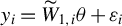 ,
$i=1,2,\ldots ,1149$
 , where
$\theta :3\times 1$
 is the unknown parameter of interest. In this model, the distribution of
$\varepsilon _{i}$
 is not specified. Moreover, the elements of
$\varepsilon _{i}$
 can be serially correlated and heteroskedastic in an arbitrary, unknown way.
BLP models: Marginal posterior distributions of the coefficient on the price variable,
$ \beta $
 . Posterior mean and standard deviation of
$ \beta $
 are
$-$
 0.089 and 0.004, respectively, for the base model with the original BLP (linear) specification, while they are
$-$
 0.087 and 0.004, respectively, with the augmented BLP (nonlinear) specification. For the extended model, posterior mean and standard deviation of
$ \beta $
 are
$-$
 0.183 and 0.015, respectively, for the linear specification and
$-$
 0.143 and 0.009, respectively, for the nonlinear specification.

Figure 4 Long description
A density plot with the x-axis labeled Effect of Price on Automobile Demand ranging from minus 0.25 to minus 0.05 and the y-axis labeled Density. The plot displays four colored distributions, each with a vertical dashed line indicating its mean.
* The Extended model, Linear specification, shown in green, is the leftmost and widest distribution, peaking near minus 0.183.
* The Extended model, Nonlinear specification, shown in yellow, is centered further to the right with a higher peak near minus 0.143.
* The Base model, Linear specification, shown in purple, is a very narrow, tall peak concentrated near minus 0.089.
* The Base model, Nonlinear specification, shown in blue, is the rightmost distribution, also very narrow and tall, peaking near minus 0.087.
The base models show much higher precision and smaller standard deviations compared to the wider, more varied extended models.
Now, let
$Z_{i} := \left (\widetilde {W}_{1,i},1,concen_{i}\right )$
 ,
$i \leq n$
 , be a
$4\times 5$
 matrix, where
$1$
 is a vector of ones, and
$concen_{i}=\left (concen_{i1},\ldots ,concen_{i4}\right ) ^{\prime }:4\times 1$
 is the vector of
$concen$
 values for route i. In the base model,
$l\,fare$
 is exogenous. The model is defined by the five moments

In the extended model, the
$l\,fare$
 moment condition is inactive. Specifically,

The ETEL-based estimation of these two models makes no assumption about the joint distribution of the cluster-level errors.
We specify the prior from a training sample. We randomly split the sample into a training sample (of say 115 clusters, equal to 10% of the total clusters) and an estimation sample (consisting of the remaining 1,034 clusters). We then estimate the base model on the training sample with a Student-t prior centered on the system wide 2SLS estimate from the training data, sd of 10 and 2.5 degrees of freedom. The posterior mean and sd are calculated from these training data under this prior. We then take the posterior mean and twice the sd from the training sample fit as the mean and sd of the prior. This determination of the prior from the training sample is helpful in the fitting, but, due to the thick tails of the prior, the information brought in by the prior pales in comparison with the information from the estimation sample.
We sample the posterior in each model by the one-block tailored MCMC algorithm. Figure 4 presents the posterior distributions from all four models. In the base model, from 10,000 MCMC draws beyond a burn-in of 1,000, we find that the posterior mean of
$\beta $
 is
$-0.551$
 and its 95% posterior credibility interval is
($-$
 0.683,
$-$
 0.419). Moreover, computation shows that
$\log (m(w_{1:n}|\mathcal {M}_{b}))=-7190.222$
 and
$\log (m(w_{1:n}|\mathcal {M}_{e})) =-7191.06$
 , signaling that
$l\,fare$
 in this problem can be viewed as exogenous.
6 CONCLUDING REMARKS
This article develops a Bayesian test for exogeneity/endogeneity of the treatment vector of interest in a linear mean regression model. This endogeneity problem is generally assumed away in the Bayesian literature, but this leads to a serious misspecification problem since endogeneity, in practice, is the rule rather than the exception. In order to avoid the risk of distributional misspecification, the framework we have developed relies only on moment restrictions. The analysis in the article revolves around the study of two models: the base model, where the exogeneity assumption is enforced, and an extended model, where the exogeneity moment is included but is made inactive.
The testing procedure for exogeneity/endogeneity is based on the Bayes factor, where the marginal ETEL of the base and the extended models are compared. The procedure is validated from a frequentist point of view because we establish the large sample consistency of the Bayes factor test. In addition, we provide a comprehensive study of the log-marginal ETEL function and determine which parts of it play a role in the testing procedure depending on whether the covariates x are exogenous or endogenous.
The real data examples discussed in the article showcase the practical relevance of the methods.
It is important to mention that the approach proposed here can be extended to situations where the controls are assumed to enter the model nonparametrically. While the finite sample analysis of such models, after approximating the unknown functions by (say) spline basis expansion methods, would proceed in much the same way as discussed in this article, the specification of the prior and the large sample analysis would require new developments to account for a growing number of basis function parameters with sample size. We intend to describe the theory in a future paper.
Another interesting extension would involve relaxing our current strong identification assumption, which is based on a fixed number of relevant instruments, to allow for weak and many-IVs. This would require substantial changes to our asymptotic results, as it would necessitate developing local-asymptotic Bayes factors for ETEL and incorporating instrument-growth penalties or shrinkage to prevent overfitting.
A APPENDIX: PROOFS OF THE MAIN RESULTS
The following notation will be used in the proofs of this section. Further notation will be introduced in Section D.1 of the Supplementary Material and will be used in the proofs there. When we omit
$y_i$
 from the vector of the i-th observation we use the notation
$\widetilde w_{i}:=(x_i',z_i')'$
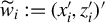 , and when in addition we omit
$z_{2,i}$
 we use the notation
$\widetilde w_{1,i}:=(x_i',z_{1,i}')'$
 . We use the notation
$\mathbf {E}_n[\cdot ]:=\frac {1}{n}\sum _{i=1}^n[\cdot ]$
 for the empirical mean. For a probability Q, we use the notation
$\mathbf {E}^{Q}[\cdot ]$
 to denote the expectation with respect to Q and
$\mathbb {V}ar_Q$
 the variance with respect to Q. For the true distribution P:
$\mathbf {E}[\cdot ] := \mathbf {E}^P[\cdot ]$
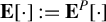 , we use the notation:
$\mathbb {P}_n: = \mathbf {E}_n[\delta _{w_i}]$
 , where
$\delta _{x}$
 is the Dirac measure at x, and
$\mathbb {G}_n f:= \sqrt {n}(\mathbf {E}_n[f] - \mathbf {E}[f])$
 for the centered empirical process, for every function f.
Let g denote a generic moment function, where
$g = g_b$
 for the base model
$\mathcal {M}_b$
 and
$g = g_e$
 for the extended model
$\mathcal {M}_e$
 . We define
$g_i(\theta ) := g(w_i,\theta )$
 the moment function evaluated at
$w_i$
 and
$\widehat \lambda (\theta ):=\widehat \lambda (w_{1:n},\theta )$
 the tilting parameter. For a function
$\lambda (\theta )$
 of
$\theta $
 , define
$\tau _i(\lambda ,\theta ):= \frac {e^{\lambda (\theta )'g_i(\theta )}}{\mathbf {E}_n[ e^{\lambda (\theta )'g_j(\theta )}]}$
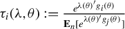 ,
$\tau _i^{\dagger }(\lambda ,\theta ):= \frac {e^{\lambda (\theta )'g_i(\theta )}}{\mathbf {E}[ e^{\lambda (\theta )'g_j(\theta )}]}$
 ,
$\tau _i^{\diamond }(\lambda ,\theta ) := e^{\lambda (\theta )'g_i(\theta )}$
 , so that
$\tau _i(\widehat \lambda ,\theta ) = n \widehat {p}_i(\theta )$
 and
$\tau _i^{\dagger }(\lambda _*,\theta ) = dQ^*(\theta )/dP$
 . We also use the notation:
$\Omega _*^{\diamond }(\lambda , \theta ) := \mathbf {E}[\tau _i^{\diamond }(\lambda ,\theta )\varepsilon _i(\theta )^2\widetilde {w}_i \widetilde {w}_i']$
 ,
$\Omega _*^{\diamond }(\theta ) := \Omega _*^{\diamond }(\lambda _*, \theta )$
 ,
$\Omega _*^{\dagger }(\theta ) := \mathbf {E}[\tau _i^{\dagger }(\lambda _*,\theta )\varepsilon _i(\theta )^2\widetilde {w}_i \widetilde {w}_i'] = \mathbf {E}^{Q^*(\theta )}[\varepsilon _i(\theta )^2\widetilde {w}_i \widetilde {w}_i']$
 , and
$\Omega _\circ := \mathbf {E}[\varepsilon _i(\theta _\circ )^2\widetilde {w}_i \widetilde {w}_i']$
 . Moreover,
$\Omega _* \equiv \Omega _*^{\diamond }(\theta _\circ )$
 .
A.1 Proof of Theorem 4.1
We first show that (i) is equivalent to (ii). Let
$H_{\infty }:=\{\theta \in \Theta; \mathcal {Q}_{b}(\theta ) \neq \emptyset \}$
 . Suppose (i) is true. Then,
$P\notin \mathcal {Q}_{b}(\theta )$
 for every
$\theta \in \Theta $
 and the I-projection of P on the set
$\mathcal {Q}_{b}(\theta )$
 is different from P, that is, for every
$\theta \in H_{\infty }$
 ,
$Q_b^*(\theta )\neq P$
 and
$KL(Q_b^*(\theta )||P)>0$
 , and it is not defined for every
$\theta \in \Theta \setminus H_{\infty }$
 because for these values of
$\theta $
 , the set
$\mathcal {Q}_b^*(\theta )$
 is empty. It follows that also the reverse KL divergence (where we have inverted the role played by the two probabilities) is strictly positive under Assumption 1:
$\mathrm {KL}(P||Q_b^*(\theta ))>0$
 for every
$\theta \in H_{\infty }$
 . Since this is true for every
$\theta \in H_{\infty }$
 , it is also true for
$\theta _*$
 . Hence, (ii) holds.
Now, suppose that (ii) is true. Because
$\mathrm {KL}(P||Q_b^*(\theta _*))>0$
 , then
$P\neq Q_b^*(\theta _*)$
 and so
$P\notin \mathcal {Q}_{b}(\theta _*)$
 . Since
$\theta _*$
 minimizes
$\mathrm {KL}(P||Q_b^*(\theta ))$
 over all the
$\theta $
 s for which
$\mathcal {Q}_{b}(\theta ) \neq \emptyset $
 , then we also have that
$P\notin \mathcal {Q}_{b}(\theta )$
 for every
$\theta \in \Theta $
 such that
$\mathcal {Q}_{b}(\theta )\neq \emptyset $
 . Since for the
$\theta $
 s for which
$\mathcal {Q}_{b}(\theta )= \emptyset $
 the condition (i) trivially holds then we have proved that (i) holds for every
$\theta \in \Theta $
 .
Next, we show that (iii) is equivalent to (iv). Suppose (iii) holds. Then, there is a
$\theta \in \Theta $
 , say
$\theta _*$
 , for which
$P\in \mathcal {Q}_{b}(\theta _*)$
 . Hence,
$Q_b^*(\theta _*) = P$
 and
$\mathrm {KL}(P||Q_b^*(\theta )) = 0$
 . Hence, (iv) holds.
Now, suppose that (iv) holds. By the properties of the KL divergence,
$\mathrm {KL}(P||Q_b^*(\theta _*))\, =\, 0$
 if and only if
$P=Q_b^*(\theta _*)$
 . It follows that
$P\in \mathcal {Q}_{b}(\theta _*)$
 because
$Q_b^*(\theta _*)\in \mathcal {Q}_{b}(\theta _*)$
 , and therefore, P satisfies the moment restriction
$\mathbf {E}^P[\varepsilon _{i}(\theta _*)x_{i}] = 0$
 . Hence, (iii) holds.
A.2 Proof of Theorem 4.2
Let us consider the expression for the likelihood evaluated at
$\theta _*$
 :

where
$\widetilde {g}_b(w_i,\theta _*) := g_b(w_i,\theta _*) - \mathbf {E}[g_b(w_i,\theta _*)]$
 . We first deal with the second term on the right-hand side of (A.1). By using the result of Lemma D.4 in the Supplementary Material,

Next, we analyze the fourth term on the right-hand side of (A.1). Let
$\widetilde \lambda $
 be on the line joining
$\lambda _*(\theta _*)$
 and
$\widehat \lambda (\theta _*)$
 , then a second-order Taylor expansion of
$\lambda \mapsto \frac {1}{n}\sum _{j=1}^n e^{\lambda ' g_b(w_j,\theta _*)}$
 around
$\lambda _*(\theta _*)$
 gives

Under Assumption 4 and because
$\|\tilde \lambda - \lambda _*(\theta _*)\|_2 = \mathcal {O}_p(n^{-1/2})$
 (since by Lemma D.3 in the Supplementary Material
$\|\widehat \lambda (\theta _*) - \lambda _*(\theta _*)\|_2 = \mathcal {O}_p(n^{-1/2})$
 and
$\tilde \lambda = \tau (\widehat \lambda (\theta _*) - \lambda _*(\theta _*)) + \lambda _*(\theta _*)$
 for some
$\tau \in [0,1]$
 ) we can apply the same argument as in the proof of Lemma D.6 in the Supplementary Material to get

By replacing this in (A.3) and by using Lemma D.3 in the Supplementary Material to get the rate of the term
$o_p(1/n)$
 term, we obtain

We now use the first-order Taylor expansion of the function
$u\mapsto \log (u)$
 around
$u_1$
 :
$\log (u) = \log (u_1) +\frac {u-u_1}{u_1} + o(|u-u_1|)$
 , and plug (A.5) in it to obtain

where to get the term
$o_p\left (\frac {1}{n}\right )$
 , we have used Lemma D.3 in the Supplementary Material and the fact that
$|\mathbf {E}_n\left [ e^{\lambda _*(\theta _*)' g_b(w_i,\theta _*)}\right ] - \mathbf {E}\left [ e^{\lambda _*(\theta _*)' g_b(w_i,\theta _*)}\right ]| = \mathcal {O}_p(1/\sqrt {n})$
 . By using again the latter convergence to show that
$\tau _i(\lambda _*,\theta _*)\xrightarrow {p} \tau _i^{\dagger }(\lambda _*,\theta _*)$
 , Lemma D.4 in the Supplementary Material, and the facts that
$\mathbf {E}[\tau _i^{\dagger }(\lambda _*,\theta _*) g_b(w_i,\theta _*)] = 0$
 and

then

Finally, we have to deal with
$\left |\frac {1}{n}\sum _{i=1}^n e^{\widehat \lambda (\theta _*)' g_b(w_i,\theta _*)} - \mathbf {E}_n\left [ e^{\lambda _*(\theta _*)' g_b(w_i,\theta _*)}\right ]\right |$
 inside the
$\mathcal {o}(\cdot )$
 term in (A.6). By using (A.5) and (A.7), we get that
$\left |\frac {1}{n}\sum _{i=1}^n e^{\widehat \lambda (\theta _*)' g_b(w_i,\theta _*)} - \mathbf {E}_n\left [ e^{\lambda _*(\theta _*)' g_b(w_i,\theta _*)}\right ]\right | = \mathcal {O}_p(1/n)$
 .
By replacing this result, (A.2), (A.6), and (A.7) in (A.1), we get

where
$\mathbb {G}_n\left [\tau _i^{\dagger }(\lambda _*,\theta _*) g_b(w_i,\theta _*)\right ] \xrightarrow {d} \mathcal {N}(0,\Omega _*^{\dagger }(\theta _*))$
 . By noticing that
$\lambda _*(\theta _*)'\sum _{i=1}^n \widetilde g_b(w_i,\theta _*) - n\log \left (\mathbf {E}_n\left [ e^{\lambda _*(\theta _*)' g_b(w_i,\theta _*)}\right ]\right ) = \sum _{i=1}^n \log \left (\tau _i(\lambda _*,\theta _*)\right ) - n\lambda _*(\theta _*)'\mathbf {E}[g_b(w_i,\theta _*)]$
 , we prove (4.3).
The last part of the theorem follows from Lemma D.4 in the Supplementary Material.
A.3 Proof of Theorem 4.3
Since we are in the extended model, then there exists a
$\psi _\circ := (\theta _\circ ', v_\circ ')'$
 such that
$\mathbf {E}[\varepsilon _i(\theta _\circ )\widetilde w_i] = (v_\circ ',0')'$
 and
$\lambda _*(\psi _\circ ) = 0$
 . Let us consider the expression for the likelihood evaluated at
$\psi _\circ $
 :

We start with dealing with the second term on the right-hand side of (A.9). By using the result of Lemma D.17 in the Supplementary Material,

Let
$\widetilde \lambda $
 be on the line joining
$0$
 and
$\widehat \lambda (\psi _\circ )$
 , then a second-order Taylor expansion of the function
$\lambda \mapsto \frac {1}{n}\sum _{j=1}^n e^{\lambda 'g_e(w_j,\theta _\circ )}$
 around
$0$
 gives

Under Assumption 4 and because
$\tilde \lambda = \mathcal {O}_p(n^{-1/2})$
 (since by Lemma D.18 in the Supplementary Material
$\widehat \lambda (\psi _\circ ) = \mathcal {O}_p(n^{-1/2})$
 and
$\widetilde \lambda $
 is between
$0$
 and
$\widehat \lambda (\psi _\circ )$
 ), we can apply the same argument as in the proof of Lemma D.6 in the Supplementary Material to get

By replacing this in (A.11) and by using Lemma D.18 in the Supplementary Material to get the rate of the
$o_p(1/n)$
 term, we obtain

We now use the first-order Taylor expansion of the function
$u\mapsto \log (u)$
 around
$1$
 :
$\log (u) = u-1 + o(|u-1|)$
 and apply it to u given by the left- hand side of (A.13) to obtain

By using the result of Lemma D.17 in the Supplementary Material and the fact that
$\mathbf {E}[g_e(w_i,\psi _\circ )] = 0$
 , then

Finally, we have to deal with
$\left |\frac {1}{n}\sum _{i=1}^n e^{\widehat \lambda (\psi _\circ )' g_e(w_i,\psi _\circ )} - 1\right |$
 . By (A.14) and (A.15), we get that
$\left |\frac {1}{n}\sum _{i=1}^n e^{\widehat \lambda (\psi _\circ )' g_e(w_i,\psi _\circ )} - 1\right | = \mathcal {O}_p(1/n)$
 .
By replacing this result and (A.15) in (A.14), and then by plugging (A.10) and (A.14) in (A.9), we get

Moreover, by the central limit theorem,

and

A.4 Proof of Corollary 4.1
By result (4.3) in Theorem 4.2, we have that

By Lemma D.3 in the Supplementary Material,
$\|\widehat \lambda (\theta _*) - \lambda _*(\theta _*)\|_2\xrightarrow {p} 0$
 . By the Law of Large Numbers,

This concludes the proof.
A.5 Proof of Corollary 4.2
By result (4.4) in Theorem 4.3, we have that

Since
$\lambda _*(\psi _\circ ) = 0$
 then,
$\frac {e^{\lambda _*(\psi _\circ )'\sum _{i=1}^n g_b(w_i,\psi _\circ )}}{\mathbf {E}[e^{\lambda _*(\psi _\circ )'\sum _{j=1}^n g_b(w_j,\psi _\circ )}]} = 1$
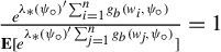 and so we can equivalently write

By the Law of Large Numbers,

This concludes the proof.
A.6 Proof of Theorem 4.4
The proof is organized in two parts. In the first part, we show that
$\mathrm {KL}(P||Q_{e}^{*}(\psi _\circ )) < \mathrm {KL}(P||Q_b^{*}(\theta _{*}))$
 if and only if there is no
$\theta $
 such that
$\mathbf {E}[\varepsilon _{i}(\theta )x_i]=0$
 . In the second part, we show that

if and only if
$\mathrm {KL}(P||Q_{e}^{*}(\psi _\circ )) < \mathrm {KL}(P||Q_b^{*}(\theta _{*}))$
 .
A.6.1 First Part
We first prove that
$\mathrm {KL}(P||Q_{e}^{*}(\psi _\circ )) < \mathrm {KL}(P||Q_b^{*}(\theta _{*}))$
 if and only if there is no
$\theta \in \Theta $
 such that
$\mathbf {E}[\varepsilon _{i}(\theta )x_i]=0$
 . Notice that
$\mathrm {KL}(P||Q_{e}^{*}(\psi _\circ ))=0$
 . Suppose that
$\mathrm {KL}(P||Q_{e}^{\ast }(\psi _\circ ))<\mathrm {KL}(P||Q_b^{\ast }(\theta _{*}))$
 and suppose that there exists a
$\theta \in \Theta $
 such that
$\mathbf {E}[\varepsilon _{i}(\theta )x_i] = 0$
 so that
$P\in \mathcal {Q}_{b}(\theta )$
 . By Assumption 2 with
$\theta _*$
 replaced by
$\theta _\circ $
 , then this
$\theta $
 must be equal to
$\theta _\circ $
 , which in turn equals
$\theta _*$
 . It follows that
$P\in \mathcal {Q}_{b}(\theta _*)$
 and by definition of
$Q_b^{\ast }(\theta _{*})$
 :
$Q_b^{\ast }(\theta _{*})=P$
 since
$Q_b^{\ast }(\theta _{*})$
 is the closest to P, in the KL sense, among all the distributions in
$\mathcal {Q}_{b}(\theta _*)$
 . Hence,
$\mathrm {KL}(P||Q_b^{\ast }(\theta _{*}))=0$
 . But this contradicts, the assumption that
$\mathrm {KL}(P||Q_{e}^{\ast }(\psi _\circ ))<\mathrm {KL}(P||Q_b^{\ast }(\theta _{*}))$
 . Hence, there is no
$\theta \in \Theta $
 such that
$\mathbf {E}[\varepsilon _{i}(\theta )x_i]=0$
 .
We now prove the reverse implication. Suppose that there is no value
$\theta \in \Theta $
 such that
$\mathbf {E}[\varepsilon _{i}(\theta )x_i]=0$
 . Hence,
$P\notin \mathcal {Q}_{b}(\theta )$
 for every
$\theta \in \Theta $
 , which implies
$P\notin \mathcal {Q}_{b}(\theta _*)$
 and
$\mathrm {KL}(P||Q_b^{*}(\theta _*))> 0$
 . On the other hand, there exists a unique
$\psi _\circ \in \mathbb {R}^{d_x}$
 such that
$P\in \mathcal {Q}_{e}(\psi _\circ )$
 since
$\mathcal {M}_e$
 is always correctly specified. This implies that
$\mathrm {KL}(P||Q_{e}^{*}(\psi _\circ )) = 0$
 and so
$\mathrm {KL}(P||Q_{e}^{*}(\psi _\circ )) < \mathrm {KL}(P||Q_b^{*}(\theta _*))$
 .
A.6.2 Second Part
We show that
$P\left (\log m(w_{1:n}|\mathcal {M}_{e})> \log m(w_{1:n}|\mathcal {M}_{b})\right ) \rightarrow 1$
 if and only if
$\mathrm {KL}(P||Q_{e}^{*}(\psi _\circ ))\, <\, \mathrm {KL}(P||Q_b^{*}(\theta _{*}))$
 . By Theorems 4.2 and 4.3, and Theorems D.6 and D.7 in the Supplementary Material and by (4.1) and (4.2), then (4.9) and (4.10) hold. By (4.9), the
$\log m(w_{1:n}|\mathcal {M}_b)$
 is equal to

and by (4.10),
$\log m(w_{1:n}|\mathcal {M}_e) = -n\log (n) - \frac {p+d_x}{2}\log (n) + \mathcal {O}_p(1)$
 . Hence, since from the Law of Large Numbers,

it follows that

where we have used Lemma D.3 in the Supplementary Material to control
$\sqrt {n}(\widehat \lambda (\theta _*) - \lambda _*(\theta _*))$
 . Suppose that
$\mathrm {KL}(P||Q_b^*(\theta _*))>0$
 , then the previous probability converges to
$1$
 . On the other hand, suppose that
$P\left (0> - \mathrm {KL}(P||Q_b^*(\theta _*)) + \mathcal {O}_p(\log (n)/\sqrt {n})\right ) \rightarrow 1$
 as
$n\rightarrow \infty $
 . This is possible only if
$\mathrm {KL}(P||Q_b^*(\theta _*))>0$
 . By the first part of the proof
$\mathrm {KL}(P||Q_b^*(\theta _*))>0$
 , if and only if there is no
$\theta $
 such that
$\mathbf {E}[\varepsilon _{i}(\theta )x_i]=0$
 .
We now prove the last assertion of the theorem. In the case, where there is a
$\theta _{\circ }$
 such that
$\mathbf {E}[\varepsilon _{i}(\theta _\circ )x_i]=0$
 , then
$\mathrm {KL}(P||Q_b^*(\theta _\circ ))=0$
 and the probability
$P (0> - \mathrm {KL}(P||Q_b^*(\theta _*)) + \mathcal {O}_p(\log (n)/\sqrt {n}) )$
 is equal to zero as
$n\rightarrow \infty $
 . This concludes the proof.
A.7 Proof of Theorem 4.5
We start by supposing that
$\mathbf {E}[\varepsilon _i(\theta _\circ ) x_i] = 0$
 . In this case,
$\theta _* = \theta _\circ $
 ,
$\lambda _*(\theta _*) = \lambda _*(\theta _\circ ) = 0$
 and by Theorems 4.2 and 4.3,

Let
$\pi _{h_{\theta }}^n(\cdot |w_{1:n},\mathcal {M}_b)$
 and
$\pi _{h_{\psi }}^n(\cdot |w_{1:n},\mathcal {M}_e)$
 denote the posterior density of
$h_{\theta }$
 and
$h_{\psi }$
 , respectively. By Corollary D.1 in the Supplementary Material (which is valid if
$\mathbf {E}[\varepsilon _i(\theta _\circ ) x_i] = 0$
 holds),

and by Theorem D.7 in the Supplementary Material,

where
$V_{\theta _\circ }$
 and
$V_{\psi _\circ }$
 are defined in Corollary D.1 and Theorem D.7 in the Supplementary Material. Hence, by replacing (A.18), (A.19), and (A.20) in
$\log m(w_{1:n}|\mathcal {M}_b) - \log m(w_{1:n}|\mathcal {M}_e)$
 by using the expressions for the log-marginal likelihoods given in (4.1) and (4.2) with
$\theta _*$
 replaced by
$\theta _\circ $
 , we obtain

Because
$\mathbb {G}_n\left [\varepsilon _i(\theta _\circ )\widetilde {w}_i\right ] = \mathcal {O}_p(1)$
 ,
$|V_{\theta _\circ }^{-1}| = \mathcal {O}(1)$
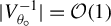 and
$|V_{\psi _\circ }^{-1}| = \mathcal {O}(1)$
 (since
$V_{\theta _\circ }$
 and
$V_{\psi _\circ }$
 are positive definite under Assumption 5), then we can factorize
$\log (n)$
 in (A.21) and get

as
$n\rightarrow \infty $
 . This proves the first implication.
We now prove the reverse implication. Suppose that
$P (\log m(w_{1:n}|\mathcal {M}_b)> \log m(w_{1:n}|\mathcal {M}_e) ) \rightarrow 1$
 . By (4.1) and (4.2),

By using Theorems 4.2 and 4.3, we get

where
$\mathcal {A}_n := \mathbb {G}_n\left [\tau _i^{\dagger }(\lambda _*,\theta _*) g_b(w_i,\theta _*)'\right ] \xrightarrow {d} \mathcal {N}(0,\Omega _*^{\dagger }(\theta _*))$
 ,
$\mathcal {B}_n := \mathbb {G}_n\left [g_b(w_i,\theta _*)'\right ] \xrightarrow {d} \mathcal {N}(0,\mathbf {E}[\varepsilon _i(\theta _\circ )]\widetilde {w}_i\widetilde {w}_i')$
 and
$\mathbb {G}_n\left [g_e(w_i,\psi _\circ )'\right ] \Omega _{\psi _\circ }^{-1} \mathbb {G}_n\left [g_e(w_i,\psi _\circ )\right ]\xrightarrow {d} \chi _{d}^2$
 and so they are bounded in probability. Moreover, by the Law of Large Numbers,

where
$\mathbf {E}\left [\log (dQ_b^*(\theta _*)/dP)\right ] = - \mathrm {KL}(P||Q_b^*(\theta _*))$
 , and by Lemma D.4 in the Supplementary Material,

Therefore,

By replacing (A.26) in (A.24), and by using Theorems D.6 and D.7 in the Supplementary Material to show that
$\log \pi _{h_{\theta }}^n(0|w_{1:n},\mathcal {M}_b) = \mathcal {O}_p(1)$
 and
$\log \pi _{h_{\psi }}^n(0|w_{1:n},\mathcal {M}_e) = \mathcal {O}_p(1)$
 , the expression in (A.24) is equal to

where
$\mathcal {O}_p(1)\sqrt {n} - n\mathrm {KL}(P||Q_b^*(\theta _*))$
 in the left-hand side converges to
$-\infty $
 if
$\mathrm {KL}(P||Q_b^*(\theta _*))>0$
 (since the term in n is diverging faster than the term in
$\sqrt {n}$
 ) while the term on the right-hand side also converges towards
$-\infty $
 . The inequality is then satisfied with probability approaching
$1$
 only if
$\mathrm {KL}(P||Q_b^*(\theta _*)) = 0$
 . This is equivalent to have
$\mathbf {E}[\varepsilon _i(\theta _\circ ) x_i] = 0$
 (by the first part of the proof of Theorem 4.4) and we have proved the second part of the “if and only if” statement.
SUPPLEMENTARY MATERIAL
The supplementary material for this article can be found at https://doi.org/10.1017/S0266466626100644.
FUNDING STATEMENT
A.S. gratefully acknowledges financial support from Hi!Paris, and ANR-21-CE26-0003.
COMPETING INTERESTS
The authors declare that no competing interests exist.