1 Introduction
Both in nature and in industrial applications, one regularly finds small inertial particles embedded in turbulent flows. By small inertial particles, we mean particles that are smaller than the smallest scales of the turbulence and have significantly higher material density than the fluid. For such particles, there will be momentum exchange between the particles and the turbulent fluid, and, depending on the conditions, there may also be heat and mass transfer. This is particularly so for chemically reacting particles, but there are also a large number of other applications where heat and mass transfer between particles and fluid are important. Here, the main focus will be on reacting particles that consume one or more of the species in the embedding gas through surface reactions. Relevant examples are chemical reactions on the surface of a catalytic particle, fuel oxidation on the surface of an oxygen carrying particle in a chemical looping combustion reactor, condensation of water vapour on cloud droplets and combustion or gasification of char.
The presence of turbulence in a fluid will enhance the transport properties of the flow. This means that the mean-field viscosity, diffusivity and conductivity may be drastically increased from their laminar values. This effect has been studied for many years, and a large number of different models exist in the literature, such as the
 $k$
-
 $\unicode[STIX]{x1D716}$
model (Jones & Launder Reference Jones and Launder1972) and different versions of the Reynolds stress models (e.g. Pope Reference Pope2003). Turbulence may also modify gas phase combustion, and even though this is somewhat more complicated, a significant number of models have been developed during the last decades. Some examples are the eddy dissipation model (Magnussen & Hjertager Reference Magnussen and Hjertager1976), the eddy dissipation concept (Ertesvåg & Magnussen Reference Ertesvåg and Magnussen2000) and variations of probability density function (e.g. Dopazo Reference Dopazo, Libby and Williams1994) models.
With the above knowledge in mind, it is interesting to realize that, except for the recent work of Kruger et al. (Reference Kruger, Haugen, Løvas and Mitra2017), there is currently no model describing the effect of turbulence on the heat and mass transfer of small inertial particles. When a reacting particle is embedded in a turbulent flow, the turbulence can potentially influence the mass transfer, and hence the surface reaction rates in two ways. The first way is through particle clustering, where particles form dense clusters due to turbulence, and where the gas phase reactants within the cluster are quickly consumed while there are no particles that can consume the reactants in the particle voids outside the clusters. The main effect of the clustering is to decrease the overall mass transfer rate. The second way turbulence influences the mass transfer rate is by increasing the mean velocity difference between the particle and the gas. This effect will increase the mass transfer rate.
The same two effects are also active for the heat transfer. The similarity between heat and mass transfer can be seen by considering the expressions for the transfer coefficients of mass,
 $$\begin{eqnarray}\displaystyle \unicode[STIX]{x1D705}=\frac{ShD}{d_{p}}, & & \displaystyle\end{eqnarray}$$
and heat,
 $$\begin{eqnarray}\displaystyle \unicode[STIX]{x1D705}_{th}=\frac{NuD_{th}}{d_{p}}, & & \displaystyle\end{eqnarray}$$
where
 $d_{p}$
is the particle diameter,
 $Sh$
and
 $Nu$
are the Sherwood and Nusselt numbers and
 $D$
and
 $D_{th}$
are the mass and thermal diffusivities. For single spherical particles in flows with low and medium particle Reynolds numbers, where the particle Reynolds number
 $Re_{p}$
is given by (2.11), the Sherwood and Nusselt numbers can be approximated by the empirical expressions of Ranz & Marshall (Reference Ranz and Marshall1952):
 $$\begin{eqnarray}\displaystyle \left.\begin{array}{@{}c@{}}Sh=2+0.69Re_{p}^{1/2}Sc^{1/3},\\ Nu=2+0.69Re_{p}^{1/2}Pr^{1/3},\end{array}\right\} & & \displaystyle\end{eqnarray}$$
where
 $$\begin{eqnarray}\displaystyle Sc=\unicode[STIX]{x1D708}/D & & \displaystyle\end{eqnarray}$$
is the Schmidt number and
 $$\begin{eqnarray}\displaystyle Pr=\unicode[STIX]{x1D708}/\unicode[STIX]{x1D6FC} & & \displaystyle\end{eqnarray}$$
is the Prandtl number, while
 $\unicode[STIX]{x1D708}$
is the viscosity and
 $D$
and
 $\unicode[STIX]{x1D6FC}$
are the mass and thermal diffusivities, respectively.
A well-known example where reacting particles are consumed in a turbulent fluid is the case of pulverized coal combustion, where turbulence influences the process in several ways that are understood to varying degrees. The combustion of coal can be divided into four separate processes: (i) drying, (ii) devolatilization, (iii) combustion of volatiles and (iv) burnout of the remaining char. Processes (i) and (ii) involve the evaporation of fluids and thermal cracking of hydrocarbons, while process (iii) involves homogeneous reactions. In process (iv), gas phase species diffuse to the particle surface and react with the solid carbon. This happens via adsorption of e.g. an oxygen radical to a carbon site on the particle surface and a subsequent desorption of carbon monoxide into the gas phase. This makes process (iv) dominated by heterogeneous chemical reactions. Many published studies utilize Reynolds averaged Navier–Stokes (RANS) based simulation tools that describe simulations of pulverized coal conversion in the form of combustion or gasification with an Eulerian–Eulerian approach (Gao et al. Reference Gao, Xu, Lin and Yang2004; Zhang et al. Reference Zhang, Wei, Zhou and Sheng2005) or a Lagrangian–Eulerian approach (Silaen & Wang Reference Silaen and Wang2010; Chen et al. Reference Chen, Yong and Ghoniem2012, Reference Chen, Horio and Kojima2000; Vascellari et al. Reference Vascellari, Schulze, Nikrityuk, Safronov and Hasse2014, Reference Vascellari, Roberts, Hla, Harris and Hasse2015; Klimanek et al. Reference Klimanek, Adamczyk, Katelbach-Wozniak, Wecel and Szlek2015). However, none of these papers take into account the effect of turbulence on the heterogeneous char reactions. To the knowledge of the authors, the only studies that take account of this effect are the papers of Luo et al. (Reference Luo, Wang, Fan and Yi2012), Brosh & Chakraborty (Reference Brosh and Chakraborty2014), Brosh et al. (Reference Brosh, Patel, Wacks and Chakraborty2015) and Hara et al. (Reference Hara, Muto, Kitano, Kurose and Komori2015) where the direct numerical simulation (DNS) approach is used. In a DNS, all turbulence scales are explicitly resolved on the computational grid, such that the effect of turbulence is implicitly accounted for. However, the DNS approach is extremely costly and can therefore only be used for small simulation domains. For simulations of large scale applications, the RANS or LES (large eddy simulation) based simulation tools will therefore be the only applicable tools for the foreseeable future.
In the current paper, the same framework developed by Kruger et al. (Reference Kruger, Haugen, Løvas and Mitra2017) has been used and extended. The aim of the paper is to identify the effect of turbulence on the mass and heat transfer of solid particles, and to develop models that describe this effect for all Damköhler numbers. Here, the Damköhler number is defined as the ratio between the integral time scale of the turbulence and the characteristic time scale of the chemical reactions.
2 Mathematical model and implementation
In the current work, the so called point-particle direct numerical simulation (PP-DNS) approach is used. Here, the turbulent fluid itself is solved with the DNS methodology, where all turbulent scales are resolved and no modelling is needed. The particles are however not resolved, but rather treated as point particles where the fluid–particle momentum, mass and heat interactions are modelled. The point-particle approach is a simplification that relies heavily on the quality of the models. The alternative approach, which is to resolve the particles and their boundary layer, is extremely computationally intensive and can currently not be done for more than a few hundred particles, even on the largest computers (Deen & Kuipers Reference Deen and Kuipers2014).
In this work we use the Pencil Code (The Pencil Code 2009), which is a high-order finite-difference code for compressible hydrodynamic flows on a Cartesian mesh. It is highly modular and can easily be adapted to different types of problems. The code runs efficiently under the Message Passing Interface (MPI) library on massively parallel shared- or distributed-memory computers, like e.g. large Beowulf clusters. In the Pencil Code, the fluid flow is described by the Eulerian formalism, while the Lagrangian formalism is used for the particle transport. Using the Eulerian formalism for the fluid flow is a valid approximation as long as the fluid can be assumed to be a continuum and as long as the diameter of each Lagrangian particle is not much smaller than the mean free path of a typical fluid molecule.
A number of simplifications are made in this paper. This has been done in order to make the simulations less computationally intensive, and, even more importantly, to isolate the dominating physical mechanisms. The particles are considered to be everlasting, i.e. they are not consumed. This has been done in order to get more accurate statistics for the model development, but has no effect on the results as such. The results obtained with everlasting particles are equally valid also for particles with variable radii. The reaction on the particle surface converts reactant
 $A$
to product
 $B$
:
 $$\begin{eqnarray}\displaystyle A\rightarrow B & & \displaystyle\end{eqnarray}$$
isothermally, i.e. there is no production or consumption of heat, such that only the mass transfer effect is considered. As explained in the Introduction, the effect on the heat transfer rate will be similar to the effect on the mass transfer rate. As reactant
 $A$
is converted to product
 $B$
, the thermodynamical and transport properties are not changed. The fact that the reactions are isothermal, and that the products do not influence the thermodynamical or transport properties of the gas phase in our simulations, will obviously have an influence on the results of individual runs, but it will not, however, influence the resulting model that is built in this paper. The model is made generic and independent of these kinds of application dependent properties. The reason for this is that the model, which will be used in RANS simulations of some application with particles that experience surface reactions at their solid surface, will always use the real instantaneous temperature and composition field from the RANS simulation. Furthermore, the reactions are assumed to be diffusion controlled, i.e. the chemical kinetics are infinitely fast. This has been done in order to identify the interesting effects. Note that the effects we are considering here are only affecting the transfer rates to the particles, not the chemical kinetics. This means that if the reactions were kinetics controlled, there would be no effect of the turbulence. Finally, particle collisions are ignored since, even in the densest clusters, the volume fraction of the particles is relatively small. Additionally, since particles that do collide will typically continue to stay within the cluster, allowing for particles to collide will not have an effect on the results as long as they do not agglomerate.
2.1 Fluid equations
The equations determining the motion of the carrier fluid are given by the continuity equation
 $$\begin{eqnarray}\displaystyle \frac{\unicode[STIX]{x2202}\unicode[STIX]{x1D70C}}{\unicode[STIX]{x2202}t}+\unicode[STIX]{x1D735}\boldsymbol{\cdot }(\unicode[STIX]{x1D70C}\boldsymbol{u})=0, & & \displaystyle\end{eqnarray}$$
and the Navier–Stokes equation
 $$\begin{eqnarray}\displaystyle \unicode[STIX]{x1D70C}\frac{\text{D}\boldsymbol{u}}{\text{D}t}=-\unicode[STIX]{x1D735}P+\unicode[STIX]{x1D735}\boldsymbol{\cdot }(2\unicode[STIX]{x1D707}\unicode[STIX]{x1D64E})+\unicode[STIX]{x1D70C}\boldsymbol{f}+\boldsymbol{F}. & & \displaystyle\end{eqnarray}$$
Here,
 $\unicode[STIX]{x1D70C}$
,
 $\boldsymbol{u}$
,
 $\unicode[STIX]{x1D707}=\unicode[STIX]{x1D70C}\unicode[STIX]{x1D708}$
and
 $\unicode[STIX]{x1D708}$
are the density, velocity and dynamic and kinematic viscosities of the carrier fluid, respectively. The pressure
 $P$
and the density
 $\unicode[STIX]{x1D70C}$
are related by the isothermal sound speed
 $c_{s}$
, i.e.
 $$\begin{eqnarray}\displaystyle P=c_{s}^{2}\unicode[STIX]{x1D70C}, & & \displaystyle\end{eqnarray}$$
while the traceless rate of strain tensor is given by
 $$\begin{eqnarray}\displaystyle \unicode[STIX]{x1D64E}={\textstyle \frac{1}{2}}(\unicode[STIX]{x1D735}\boldsymbol{u}+(\unicode[STIX]{x1D735}\boldsymbol{u})^{T})-{\textstyle \frac{1}{3}}\unicode[STIX]{x1D735}\boldsymbol{\cdot }\boldsymbol{u}. & & \displaystyle\end{eqnarray}$$
Kinetic energy is injected into the simulation box through the forcing function
 $f$
, which is solenoidal and non-helical and injects energy and momentum perpendicular to a random wave vector whose direction changes every time step (Haugen & Brandenburg Reference Haugen and Brandenburg2006; Haugen et al.
Reference Haugen, Kleeorin, Rogachevskii and Brandenburg2012). Similar kinds of forcing have also previously been used for particle laden flows by other groups (Bec et al.
Reference Bec, Biferale, Cencini, Lanotte, Musacchio and Toschi2007). The energy injection rate is maintained at a level such that the maximum Mach number is always below 0.5. The domain is cubic with periodic boundaries in all directions. The momentum exchange term,
 $\boldsymbol{F}$
, is chosen to conserve momentum between the fluid and the solid particles, i.e.
 $$\begin{eqnarray}\boldsymbol{F}=-\frac{1}{V_{cell}}\mathop{\sum }_{k}m^{k}\boldsymbol{a}^{k},\end{eqnarray}$$
where
 $V_{cell}$
is the volume of the grid cell of interest and
 $m^{k}$
and
 $\boldsymbol{a}^{k}$
are the mass and acceleration (due to fluid drag) of the
 $k$
th particle within the grid cell.
The equation of motion of the reactant has the well-known advection–reaction–diffusion form
 $$\begin{eqnarray}\displaystyle \frac{\unicode[STIX]{x2202}X}{\unicode[STIX]{x2202}t}+\boldsymbol{u}\boldsymbol{\cdot }\unicode[STIX]{x1D735}X=D\unicode[STIX]{x1D6FB}^{2}X+\tilde{R}, & & \displaystyle\end{eqnarray}$$
where
 $X$
,
 $\bar{M}_{c}$
and
 $D$
are the mole fraction, the mean molar mass and the diffusivity of the reactant, respectively. The last term in (2.7),
 $\tilde{R}$
, is the sink term due to the gas–solid reactions on the surface of the solid particles.
2.2 Particle equations
The
 $N_{p}$
particles that are embedded in the flow are treated as point particles, which means that they are assumed to be significantly smaller than the viscous scale of the fluid and the diffusive scale of the reactant. The motion of the
 $k$
th particle is described by the equations for position,
 $$\begin{eqnarray}\displaystyle \frac{\text{d}\boldsymbol{r}^{k}}{\text{d}t}=\boldsymbol{V}^{k}, & & \displaystyle\end{eqnarray}$$
and velocity,
 $$\begin{eqnarray}\displaystyle \frac{\text{d}\boldsymbol{V}^{k}}{\text{d}t}=\boldsymbol{a}^{k}, & & \displaystyle\end{eqnarray}$$
where the particle acceleration due to fluid drag is given by
 $\boldsymbol{a}^{k}=[\boldsymbol{u}(\boldsymbol{r}^{k})-\boldsymbol{V}^{k}]/\unicode[STIX]{x1D70F}^{k}$
. Note that gravity is neglected in this work. The particle response time is given by (Schiller & Naumann Reference Schiller and Naumann1933)
 $$\begin{eqnarray}\displaystyle \unicode[STIX]{x1D70F}^{k}=\frac{\unicode[STIX]{x1D70F}_{St}}{1+f_{c}^{k}}, & & \displaystyle\end{eqnarray}$$
where
 $\unicode[STIX]{x1D70F}_{St}=Sd_{p}^{2}/18\unicode[STIX]{x1D708}$
is the Stokes time,
 $f_{c}^{k}=0.15(Re_{p}^{k})^{0.687}$
is a Reynolds number correction term to the classical Stokes time,
 $S=\unicode[STIX]{x1D70C}_{p}/\unicode[STIX]{x1D70C}$
is the density ratio,
 $\unicode[STIX]{x1D70C}_{p}$
is the material density of the particles,
 $$\begin{eqnarray}\displaystyle Re_{p}^{k}=\frac{|\boldsymbol{u}(\boldsymbol{r}^{k})-\boldsymbol{V}^{k}|d_{p}}{\unicode[STIX]{x1D708}}=\frac{u_{rel}^{k}d_{p}}{\unicode[STIX]{x1D708}} & & \displaystyle\end{eqnarray}$$
is the particle Reynolds number of particle
 $k$
, and
 $d_{p}$
is the particle diameter.
2.3 Surface reactions
Let us now model the reactive term. We assume that the reactions are limited to the surface of the particles and that the reactions are diffusion controlled, i.e. that all reactant that reaches the particle surface is consumed immediately. (It is possible to relax the assumption of diffusion controlled reactions by also accounting for chemical kinetics at the particle surface: see Kruger et al. (Reference Kruger, Haugen, Løvas and Mitra2017).) The reactive term can then be written as
 $$\begin{eqnarray}\displaystyle \tilde{R}=\frac{1}{V_{cell}}\mathop{\sum }_{k}A_{p}^{k}\unicode[STIX]{x1D705}X_{\infty }^{k}, & & \displaystyle\end{eqnarray}$$
where
 $A_{p}=\unicode[STIX]{x03C0}d_{p}^{2}$
is the external surface area of the particle, the mass transfer coefficient is given by (1.1) and
 $Sh$
is the Sherwood number.
To couple the reactive particle with the continuum equations we use the following prescription: for the
 $k$
th particle, which is at position
 $\boldsymbol{r}^{k}$
, we set
 $$\begin{eqnarray}X_{\infty }^{k}=X(\boldsymbol{r}^{k}),\end{eqnarray}$$
i.e. the far field reactant mole fraction is set equal to the reactant mole fraction of the fluid cell where the particle is. In the current work, the particle Sherwood number is determined by the expression of Ranz & Marshall (Reference Ranz and Marshall1952) (see (1.3) in the Introduction), which is in contrast to the work of Kruger et al. (Reference Kruger, Haugen, Løvas and Mitra2017) where the Sherwood number was set to a constant value of 2, which corresponds to the Sherwood number in a quiescent flow (see (1.3)).
2.4 The reactant consumption rate
It is useful to define a reactant consumption rate as
 $$\begin{eqnarray}\displaystyle \unicode[STIX]{x1D6FC}=-\overline{\left(\frac{\tilde{R}}{X_{\infty }}\right)}=n_{p}\overline{A_{p}\unicode[STIX]{x1D705}}, & & \displaystyle\end{eqnarray}$$
where
 $\overline{O}$
represents the volume average of flow property
 $O$
and
 $n_{p}$
is the particle number density. If everything is assumed to be homogeneously distributed over the volume, the reactant consumption rate is given by
 $$\begin{eqnarray}\displaystyle \unicode[STIX]{x1D6FC}_{hom}=n_{p}A_{p}\overline{\unicode[STIX]{x1D705}}=n_{p}A_{p}\frac{\overline{Sh}D}{d_{p}} & & \displaystyle\end{eqnarray}$$
for a given diffusivity, particle size and number density. The mass transfer coefficient and Sherwood number averaged over all particles are given by
 $\overline{\unicode[STIX]{x1D705}}$
and
 $\overline{Sh}$
, respectively. The averaging should be made over the scale of the unresolved turbulent eddies.
In many RANS based simulation tools, where the local fluid velocity is not resolved, it is common to neglect the relative velocity difference between the turbulent eddies and the particles. From (1.3) it is clear that neglecting the relative velocity, which means that
 $Re_{p}=0$
, yields that
 $Sh=2$
. Since the effect of particle clustering is also neglected in such models, the modelled reactant consumption rate becomes
 $$\begin{eqnarray}\displaystyle \unicode[STIX]{x1D6FC}_{Sh,Da}=\lim _{Sh\rightarrow 2,Da\rightarrow 0}\unicode[STIX]{x1D6FC}=n_{p}A_{p}\frac{2D}{d_{p}}. & & \displaystyle\end{eqnarray}$$
In the following,
 $\unicode[STIX]{x1D6FC}_{Sh,Da}$
will be used for normalization, such that the normalized decay rate is given by
 $$\begin{eqnarray}\displaystyle \tilde{\unicode[STIX]{x1D6FC}}=\frac{\unicode[STIX]{x1D6FC}}{\unicode[STIX]{x1D6FC}_{Sh,Da}}. & & \displaystyle\end{eqnarray}$$
It is useful to define the Damköhler number, which is the ratio of the typical turbulent and chemical time scales, as
 $$\begin{eqnarray}\displaystyle Da=\frac{\unicode[STIX]{x1D70F}_{L}}{\unicode[STIX]{x1D70F}_{c}}, & & \displaystyle\end{eqnarray}$$
where
 $\unicode[STIX]{x1D70F}_{L}=L/u_{rms}$
is the integral time scale of the turbulence,
 $L$
is the turbulent forcing scale,
 $u_{rms}$
is the root-mean-square turbulent velocity and the chemical time scale is
 $$\begin{eqnarray}\displaystyle \unicode[STIX]{x1D70F}_{c}=1/\unicode[STIX]{x1D6FC}_{Sh,Da}. & & \displaystyle\end{eqnarray}$$
Particles in a turbulent flow field will tend to form clusters with higher particle number density than the average (Squires & Eaton Reference Squires and Eaton1991; Eaton & Fessler Reference Eaton and Fessler1994; Wood et al. Reference Wood, Hwang and Eaton2005; Toschi & Bodenschatz Reference Toschi and Bodenschatz2009). If the chemical time scale is short compared to the lifetime of the clusters, the reactant concentration within the clusters will be much lower than that outside the clusters. On the other hand, if the particle number density is low, the particle clusters will not have enough time to consume a significant fraction of the reactant during the lifetime of the cluster, and hence, the reactant concentration will be roughly the same inside as it is outside the clusters. By assuming that the lifetime of the clusters is of the order of the turbulent time scale, it is clear that the reactant concentration of particle flows with low Damköhler number will behave as if the particles were homogeneously distributed over the volume, i.e. for small Damköhler numbers there is no effect of particle clustering on the reactant consumption.
From (2.15)–(2.19) it can be deduced that for the homogeneous case, and then also for all cases with low Damköhler numbers, the reactant consumption rate will scale linearly with the Damköhler number for a given turbulent flow field, such that
 $$\begin{eqnarray}\displaystyle \unicode[STIX]{x1D6FC}_{hom}=\frac{Da}{\unicode[STIX]{x1D70F}_{L}}\frac{\overline{Sh}}{2}. & & \displaystyle\end{eqnarray}$$
When relaxing the restriction to small Damköhler numbers, the effect of particle clustering eventually comes into play. Kruger et al. (Reference Kruger, Haugen, Løvas and Mitra2017) have shown that the reactant consumption rate is given by
 $$\begin{eqnarray}\displaystyle \unicode[STIX]{x1D6FC}=\frac{\unicode[STIX]{x1D6FC}_{c}\unicode[STIX]{x1D6FC}_{hom}}{\unicode[STIX]{x1D6FC}_{c}+\unicode[STIX]{x1D6FC}_{hom}}, & & \displaystyle\end{eqnarray}$$
where
 $\unicode[STIX]{x1D6FC}_{c}$
is a cluster dependent decay rate. (Note that since Kruger et al. assumed the Sherwood number to be 2, their
 $\unicode[STIX]{x1D6FC}_{hom}$
equals our
 $\unicode[STIX]{x1D6FC}_{Sh,Da}=Da/\unicode[STIX]{x1D70F}_{L}$
.) From this expression, the following normalized reactant consumption rate is found to be
 $$\begin{eqnarray}\displaystyle \tilde{\unicode[STIX]{x1D6FC}}=\frac{\unicode[STIX]{x1D6FC}}{\unicode[STIX]{x1D6FC}_{Sh,Da}}=\frac{\unicode[STIX]{x1D6FC}_{c}\unicode[STIX]{x1D70F}_{L}}{\unicode[STIX]{x1D6FC}_{c}\unicode[STIX]{x1D70F}_{L}+Da\overline{Sh}/2}\frac{\overline{Sh}}{2}, & & \displaystyle\end{eqnarray}$$
where
 $Sh$
is given by (1.3) and the corresponding relative velocity between the particle and the fluid is determined by a model (which will be obtained in the next subsection). For diffusion controlled reactions, the modified reactant decay rate, as given by (2.22), is a measure of the relative modification to the mass transfer rate due to the effect of turbulence. This means that a modified Sherwood number can now be defined that accounts for the effect of turbulence:
 $$\begin{eqnarray}\displaystyle Sh_{mod}=2\tilde{\unicode[STIX]{x1D6FC}}=\overline{Sh}\frac{\unicode[STIX]{x1D6FC}_{c}\unicode[STIX]{x1D70F}_{L}}{\unicode[STIX]{x1D6FC}_{c}\unicode[STIX]{x1D70F}_{L}+Da\overline{Sh}/2}. & & \displaystyle\end{eqnarray}$$
In the limit of small Damköhler numbers, this expression reduces to
 $Sh_{mod}=\overline{Sh}$
, as expected.
By employing the modified Sherwood number given by (2.23), one can now use the common expression for the reactant consumption rate, as given by (2.15), to find the real reactant consumption rate. In most cases, however, one needs the particle conversion rate
 ${\dot{n}}_{reac}$
for individual particles, which is closely connected to the reactant decay rate. For diffusion controlled reactions, the particle conversion rate is given by
 ${\dot{n}}_{reac}=-\overline{\unicode[STIX]{x1D705}}X_{\infty }C_{g}$
, where
 $C_{g}$
is the molar concentration of the gas phase. The mass transfer coefficient is now obtained by using the modified Sherwood number in (1.1), such that
 $$\begin{eqnarray}\displaystyle \overline{\unicode[STIX]{x1D705}}=\frac{DSh_{mod}}{d_{p}}. & & \displaystyle\end{eqnarray}$$
In many applications, the reaction rate is not purely diffusion controlled. This can be accounted for by including the effect of reaction kinetics at the particle surface. The corresponding particle conversion rate can then be expressed as (Kruger et al. Reference Kruger, Haugen, Løvas and Mitra2017)
 $$\begin{eqnarray}\displaystyle {\dot{n}}_{reac}=-\frac{\unicode[STIX]{x1D706}\overline{\unicode[STIX]{x1D705}}}{\unicode[STIX]{x1D706}+\overline{\unicode[STIX]{x1D705}}}X_{\infty }C_{g}, & & \displaystyle\end{eqnarray}$$
where
 $\unicode[STIX]{x1D706}$
is the surface specific molar conversion rate. Since the reaction kinetics is only dependent on the conditions at the particle surface, the surface specific molar conversion rate is not affected by the turbulence. This is, as we have already seen, not the case for the mass transfer coefficient, which is now given by (2.24).
The main conclusion of this paper is that particles with surface reactions must account for the effect of turbulence on the mass transport to the particles. This is done by using the modified Sherwood number, as defined in (2.23). In this way, all the common machinery for calculating particle reaction rates can still be used since the effects of the turbulence are incorporated into the modified Sherwood number.
3 Results
In all of the following, statistically stationary homogeneous and isotropic turbulence is considered. The Reynolds number is varied by changing the domain size while maintaining constant viscosity and turbulence intensity. The Damköhler number is varied by changing the number of particles, while keeping everything else the same. For the simulations in this work, up to
 $12.8\times 10^{6}$
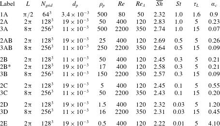
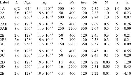
particles have been used. The accuracy of the simulations have been assessed by performing grid independence studies to verify that the turbulence is properly resolved. In addition, the number of particles has been increased to check that the results are independent of this parameter. When increasing the number of particles, the size and material density of the particles had to be augmented in order to maintain constant Damköhler and Stokes numbers. All relevant simulations are listed in table 1.
Summary of the different groups of simulations. For every row in the table, a range of simulations with different Damköhler numbers have been performed. This means that each row in the table corresponds to a given line in figures 5 and 6, while individual points in the same figures correspond to individual simulations. The fluid density is unity while the Schmidt number is 0.2 and the viscosity is
 $2\times 10^{-4}~\text{m}^{2}~\text{s}^{-1}$
for all simulations. The Taylor micro-scale Reynolds number is given by
 $Re_{\unicode[STIX]{x1D706}}=u^{\prime 2}[15/\unicode[STIX]{x1D708}\unicode[STIX]{x1D716}]^{1/2}$
where
 $u^{\prime }=u_{rms}/\sqrt{3}$
. Columns 2–5 list input parameters, while the last six columns give output from the simulations. The averaged Sherwood number for all particles is given by
 $\overline{Sh}$
. The cluster decay rate, which is defined in (3.15), is given by
 $\unicode[STIX]{x1D6FC}_{c}$
.
3.1 The mean relative particle velocity
In order to predict a representative value of the particle Sherwood number from (1.3), the particle Reynolds number
 $Re_{p}$
is required. From (2.11) it is clear that this also requires the relative particle velocity
 $u_{rel}$
, which will be found in this subsection.
Given a particle with a response time that equals the Stokes time,
 $$\begin{eqnarray}\displaystyle \unicode[STIX]{x1D70F}_{p}=\frac{Sd_{p}^{2}}{18\unicode[STIX]{x1D708}}, & & \displaystyle\end{eqnarray}$$
such that
 $\unicode[STIX]{x1D70F}_{k}<\unicode[STIX]{x1D70F}_{p}<\unicode[STIX]{x1D70F}_{L}$
, where
 $\unicode[STIX]{x1D70F}_{k}$
is the Kolmogorov time scale and
 $\unicode[STIX]{x1D70F}_{L}$
is the integral time scale. With respect to the particle–turbulence interactions, the turbulent power spectrum may be divided into three distinct regimes, based on the relation between the particle response time and the turbulent eddy turnover time
 $\unicode[STIX]{x1D70F}_{eddy}$
. The first regime is defined as the section of the turbulent power spectrum where the turbulent eddies have turnover times that are much larger than the response time of the particles, i.e. where
 $\unicode[STIX]{x1D70F}_{eddy}\gg \unicode[STIX]{x1D70F}_{p}$
. All the turbulent eddies in this regime will see the particles as passive tracers, which follow the fluid perfectly. i.e. there will be no relative velocity between the particles and the eddies. The third regime is defined as the part of the power spectrum where the turbulent eddies have much shorter time scales than the particles, i.e. where
 $\unicode[STIX]{x1D70F}_{eddy}\ll \unicode[STIX]{x1D70F}_{p}$
. The eddies in regime three will see the particles as ‘heavy bullets’ that move in straight lines, without being affected by the motion of the eddies. Hence, the velocity of these eddies will contribute to the relative particle–fluid velocity. The second regime is now defined as the relatively thin band in between regimes one and three, where
 $\unicode[STIX]{x1D70F}_{eddy}\approx \unicode[STIX]{x1D70F}_{p}$
. These are the eddies that are responsible for particle clustering, since they are able to accelerate the particles to a level where they are thrown out of the eddy due to their inertia. In the following, we will refer to a typical eddy in regime two as a resonant eddy, and we define the scale of this eddy as
 $\ell$
. The resonant eddies are identified by their time scale,
 $\unicode[STIX]{x1D70F}_{\ell }$
, which is of the order of the particle response time,
 $\unicode[STIX]{x1D70F}_{p}$
. For convenience, we set the two time scales equal, such that
 $$\begin{eqnarray}\displaystyle \unicode[STIX]{x1D70F}_{\ell }=\unicode[STIX]{x1D70F}_{p}. & & \displaystyle\end{eqnarray}$$
Based on the definitions above, it is clear that the largest turbulent eddies that yield a relative velocity between the fluid and the particles are the resonant eddies. By assuming Kolmogorov scaling, the velocity of the resonant eddies is known to be
 $u_{\ell }=u_{rms}(\ell /L)^{1/3}$
, which can be combined with the above expression for the time scales to yield
 $$\begin{eqnarray}\displaystyle k_{\ell }=k_{L}St^{-3/2}, & & \displaystyle\end{eqnarray}$$
where the particle Stokes number is defined as
 $$\begin{eqnarray}\displaystyle St=\frac{\unicode[STIX]{x1D70F}_{p}}{\unicode[STIX]{x1D70F}_{L}} & & \displaystyle\end{eqnarray}$$
and
 $k_{\ell }=2\unicode[STIX]{x03C0}/\ell$
and
 $k_{L}=2\unicode[STIX]{x03C0}/L$
are the wavenumbers of the resonant eddies and the integral scale, respectively. In obtaining (3.3), the turnover time of the resonant eddies is
 $\unicode[STIX]{x1D70F}_{\ell }=\ell /u_{\ell }$
has also been used, while that of the integral scale eddies is
 $\unicode[STIX]{x1D70F}_{L}=L/u_{rms}$
.
Since all scales smaller than
 $\ell$
will induce a relative velocity between the particles and the fluid, it is reasonable to assume that the mean relative velocity between the fluid and the particles will be a certain fraction
 $\unicode[STIX]{x1D6FD}$
of the integrated turbulent velocity
 $\tilde{u} _{\ell }$
of all scales smaller than
 $\ell$
, such that
 $$\begin{eqnarray}\displaystyle u_{rel}=\unicode[STIX]{x1D6FD}\tilde{u} _{\ell }, & & \displaystyle\end{eqnarray}$$
where
 $\tilde{u} _{\ell }$
is defined as
 $$\begin{eqnarray}\displaystyle \frac{1}{2}\tilde{u} _{\ell }^{2}=\int _{k_{\ell }}^{k_{\unicode[STIX]{x1D702}}}E(k)\,\text{d}k & & \displaystyle\end{eqnarray}$$
and
 $k_{\unicode[STIX]{x1D702}}=2\unicode[STIX]{x03C0}/\unicode[STIX]{x1D702}$
is the wavenumber of the Kolmogorov scale (
 $\unicode[STIX]{x1D702}=(\unicode[STIX]{x1D708}^{3}/\unicode[STIX]{x1D716})^{1/4}$
), where
 $\unicode[STIX]{x1D716}$
is the dissipation rate of turbulent kinetic energy. Integration of (3.6) yields
 $$\begin{eqnarray}\displaystyle \tilde{u} _{\ell }=u_{rms}\sqrt{\frac{k_{\ell }^{-2/3}-k_{\unicode[STIX]{x1D702}}^{-2/3}}{k_{L}^{-2/3}-k_{\unicode[STIX]{x1D702}}^{-2/3}}} & & \displaystyle\end{eqnarray}$$
for
 $E(k)=c\unicode[STIX]{x1D716}^{2/3}k^{-5/3}$
where we have used that the total turbulent kinetic energy is given by
 $$\begin{eqnarray}\displaystyle \frac{1}{2}u_{rms}^{2}=\int _{k_{1}}^{k_{\unicode[STIX]{x1D702}}}E(k)\,\text{d}k, & & \displaystyle\end{eqnarray}$$
where
 $k_{1}$
is the wavenumber of the largest scale in the simulation. Combining (3.3) and (3.7) with (3.5) finally yields
 $$\begin{eqnarray}\displaystyle u_{rel}=\unicode[STIX]{x1D6FD}u_{rms}\sqrt{\frac{Stk_{L}^{-2/3}-k_{\unicode[STIX]{x1D702}}^{-2/3}}{k_{L}^{-2/3}-k_{\unicode[STIX]{x1D702}}^{-2/3}}}. & & \displaystyle\end{eqnarray}$$
The unknown constant in this equation,
 $\unicode[STIX]{x1D6FD}$
, can be determined numerically from (3.5), i.e.
 $\unicode[STIX]{x1D6FD}=u_{rel}/\tilde{u} _{\ell }$
. Here, the mean relative particle velocity
 $u_{rel}$
is found directly from DNS simulations, while
 $\tilde{u} _{\ell }$
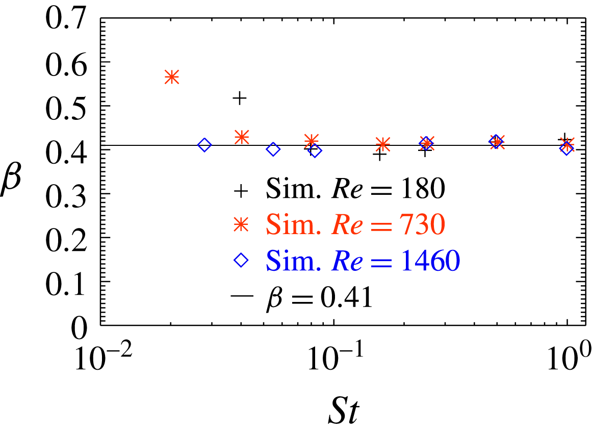
is calculated from (3.7). It is seen from figure 1 that
 $\unicode[STIX]{x1D6FD}$
is close to 0.41 for most Stokes and Reynolds numbers. The main exception is for low Reynolds and Stokes numbers, where
 $\unicode[STIX]{x1D6FD}$
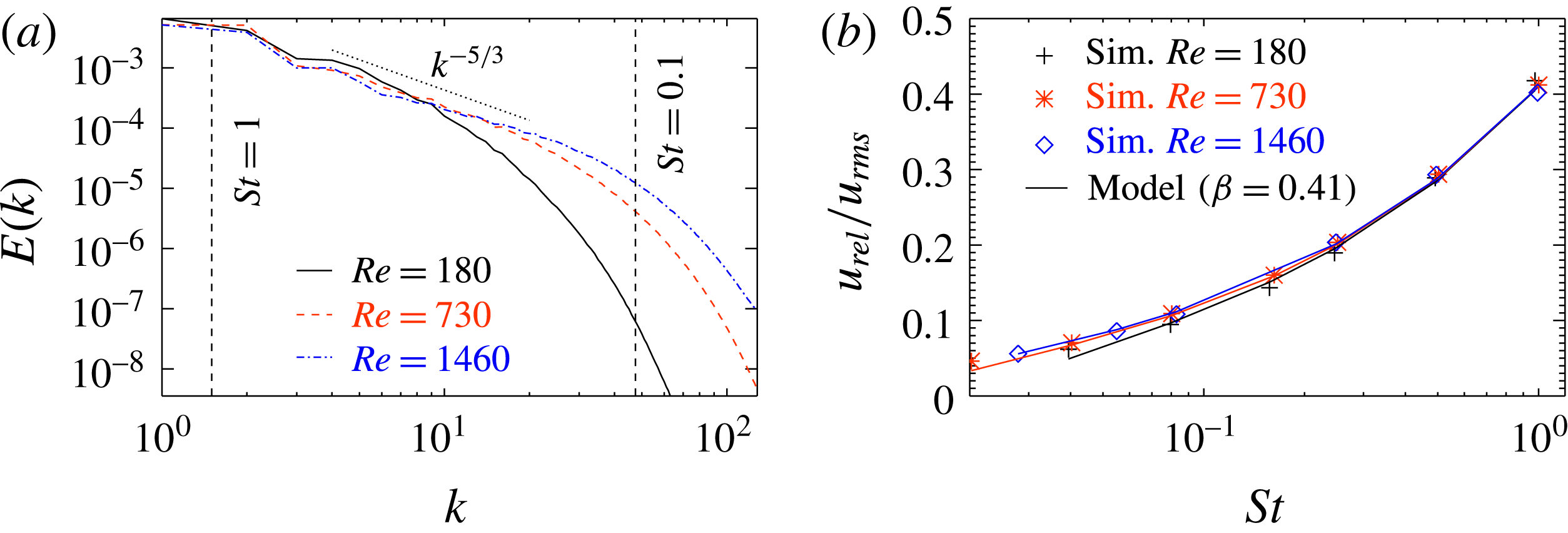
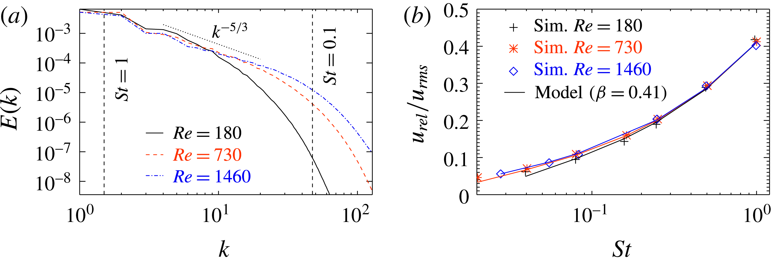
is significantly larger. This can be understood by inspecting figure 2(a), where it is seen that for
 $Re=180$
and
 $St<0.1$
, we are already far into the dissipative sub-range, where our model is not expected to be correct since it relies on a Kolmogorov scaling.
The parameter
 $\unicode[STIX]{x1D6FD}$
, relating the relative particle velocity to the sub-scale velocity as defined in (3.9), is shown for a number of different DNS simulations as a function of Stokes number.

(a) Kinetic energy spectrum for DNS simulations with different Reynolds numbers. (b) Relative particle velocity as a function of Stokes number. In (b), symbols represent simulation results, while lines correspond to the model given by (3.9) where the value of
 $\unicode[STIX]{x1D6FD}$
has been chosen to be 0.41.
It is surprising to see that (3.9) reproduces the relative particle velocity for such low Stokes numbers, even for the smaller Reynolds numbers. This may be explained by reconsidering (3.2), where we assumed that the resonant eddies correspond to the eddies that have exactly the same turnover time as the response time of the particles. This is just an order of magnitude estimate, and a more correct expression would probably be
 $$\begin{eqnarray}\displaystyle \unicode[STIX]{x1D70F}_{\ell }=\unicode[STIX]{x1D6FE}\unicode[STIX]{x1D70F}_{p}, & & \displaystyle\end{eqnarray}$$
where
 $\unicode[STIX]{x1D6FE}$
is of the order of unity. More work should, however, be devoted to understanding the coupling between the particles and the turbulent eddies. In particular, a more exact definition of the resonant eddies is needed. We nevertheless believe that
 $\unicode[STIX]{x1D6FD}$
is a universal property of the heavy inertial particles approximation and the Navier–Stokes equations that will have a constant value for all
 $Re$
and
 $St$
as long as the resonant eddies are within the inertial range.
In figure 2(b), the average relative particle velocity, as found from the DNS simulations (symbols), is compared with the predicted values from (3.9) (solid lines). It is seen that the fit is rather good for most Reynolds and Stokes numbers. This supports the use of (3.9) for predicting the relative particle velocity.
3.2 The cluster size
The typical size of the clusters
 $\ell$
is assumed to be the size of the resonant eddies. From (3.3) this yields a cluster size of
 $$\begin{eqnarray}\displaystyle \ell =LSt^{3/2}. & & \displaystyle\end{eqnarray}$$
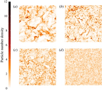
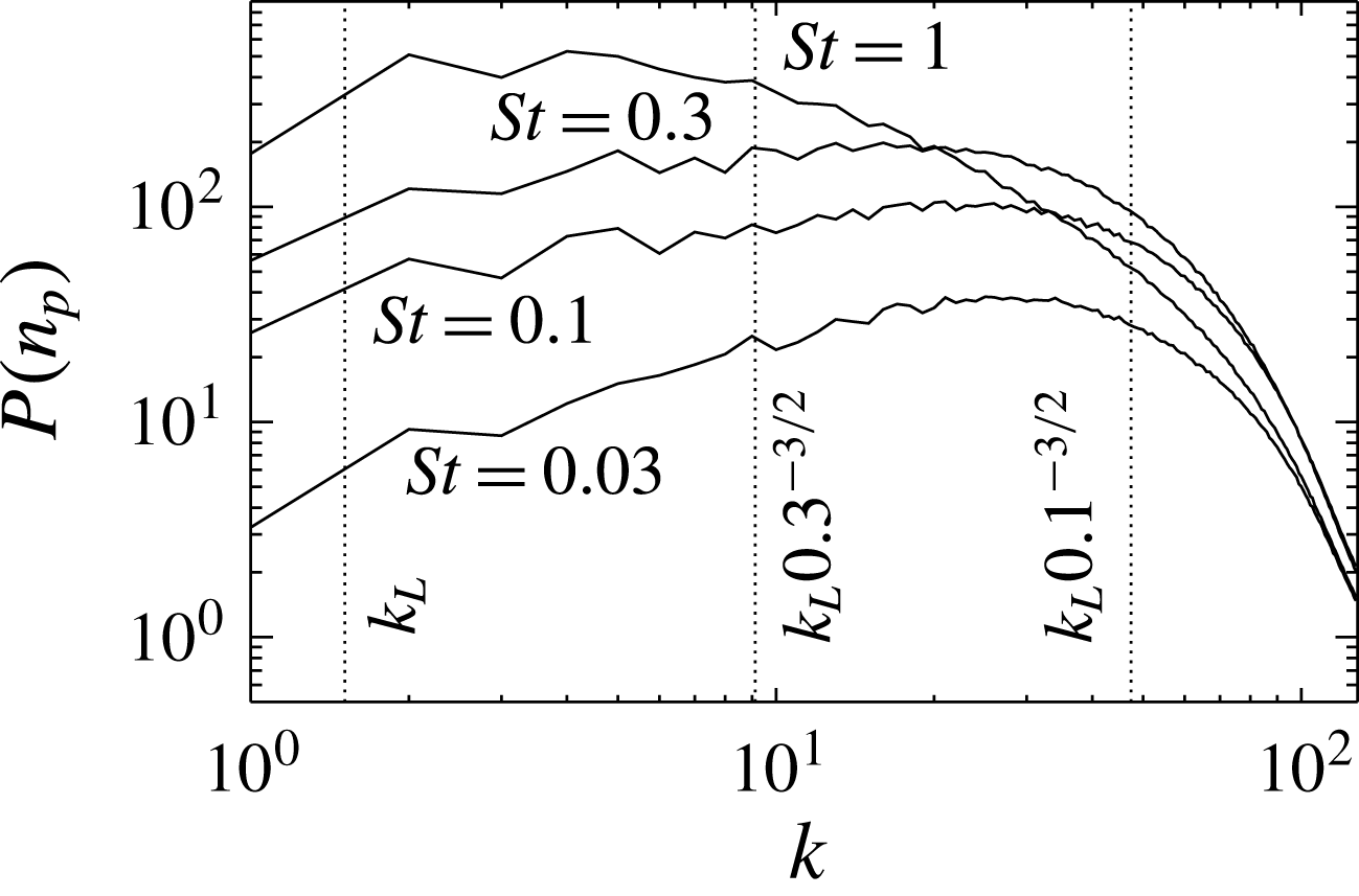
It can be seen from figure 3 that the distribution of the particle number density, which is defined as the number of particles per unit volume, does indeed show more small scale variation for the smaller Stokes numbers. This has been quantified in figure 4 where the power spectrum of the particle number density is shown. Here we see that the spectrum peaks at large scales for
 $St=1$
while the peak is located at much smaller scales for smaller Stokes numbers. The peak in the spectrum does not, however, follow (3.11) as accurately as expected. The reason for this is most likely that power spectra are not the right diagnostics to study the size of particle clusters. Alternatively, the constant in the definition of the resonant eddies may not be unity (see e.g. (3.10)). Another possible reason for the discrepancy may be finite Reynolds number effects, which means that the clustering eddies are outside, or close to being outside, the inertial range. Since (3.11) is based on Kolmogorov statistics, this would give simulation results that violate (3.11). Finally, even poor statistics due to too few particles relative to the number of clustering eddies, which means that the clusters are not populated with enough particles, may also yield results that do not follow (3.11). This can be understood by assuming a case with only two particles and a thousand clustering eddies. By visualizing a snapshot of the particle positions, it would not be possible to identify any particle cluster, because the two particles would seem to be randomly distributed. If, on the other hand, there were a thousand particles and only two turbulent eddies, it would be straightforward to see that the particles tend to cluster outside the eddies.
The power spectrum
 $P$
can be integrated to yield a measure of the strength in the particle number density fluctuations, given by the root-mean-square (r.m.s.) particle number density:
 $$\begin{eqnarray}\displaystyle n_{rms}=\int P\,\text{d}k. & & \displaystyle\end{eqnarray}$$
It is found that the r.m.s. particle number density is decreasing with Stokes number. More specifically,
 $n_{rms}$
is 1.6, 1.5, 1.2 and 0.8 for Stokes numbers of 1, 0.3, 0.1 and 0.03, respectively. This means that the high density regimes have higher particle number densities for larger Stokes numbers.
Particle number density for
 $St=1$
(a),
 $St=0.3$
(b),
 $St=0.1$
(c) and
 $St=0.03$
(d) (runs 3A, 3B, 3C and 3D in table 1). It is only the Stokes number that differs between the four simulations; all other parameters, including the total number of particles, are the same.

Power spectrum of particle number density for runs 3A, 3B, 3C and 3D in table 1.

3.3 Reactant consumption rate
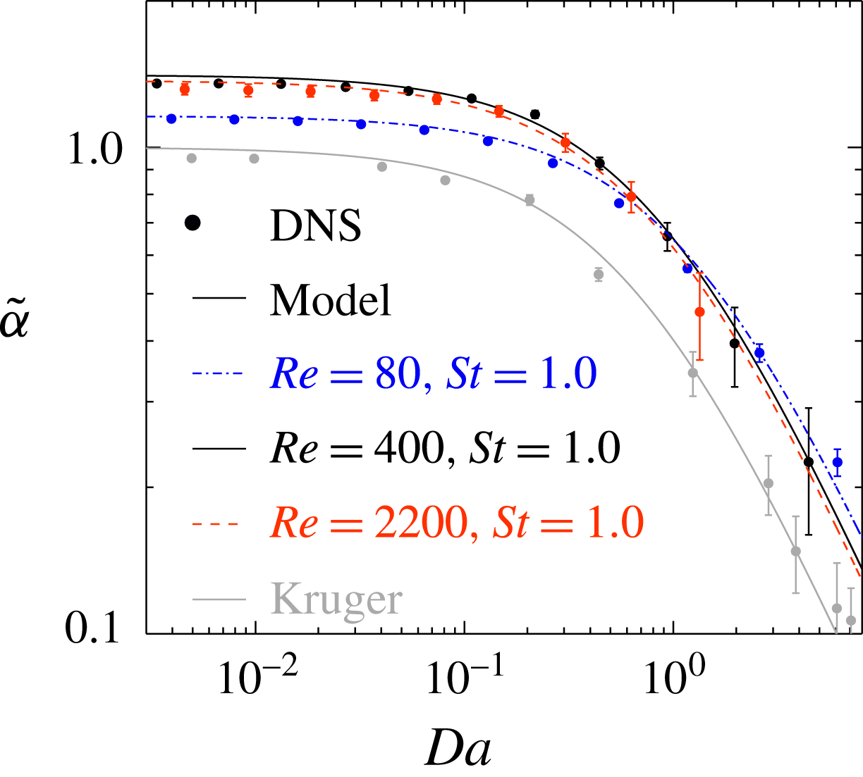
The normalized reactant consumption rate is shown in figure 5. The symbols correspond to the results from the DNS simulations, as given by (2.17), where
 $\unicode[STIX]{x1D6FC}$
is found from (2.14), while the solid lines are given by (2.22). Here, the Stokes number is found by using the model for the relative velocity, as given by (3.9), in the expression for the Sherwood number (1.3). The value of the cluster decay rate,
 $\unicode[STIX]{x1D6FC}_{c}$
, is the only free parameter and it is chosen by a best fit approach between the DNS results (2.14) and the model results (2.21) for
 $\unicode[STIX]{x1D6FC}$
. The values of
 $\unicode[STIX]{x1D6FC}_{c}$
are found in table 1.
The value of
 $\tilde{\unicode[STIX]{x1D6FC}}$
for small Damköhler numbers equals the Sherwood number divided by two, while the Damköhler number for which
 $\tilde{\unicode[STIX]{x1D6FC}}$
starts to decrease is determined by the cluster decay rate
 $\unicode[STIX]{x1D6FC}_{c}$
. Overall, the model seems to follow the results from the DNS simulations rather well.
From figure 5 it can be seen that for large Stokes numbers, the curves for the normalized decay rates of a given Stokes number overlap for different Reynolds numbers if the Reynolds number is high enough. This is because the resonant eddies are at scales larger than the dissipative sub-range. So increasing the Reynolds number, which may be considered a shift of the dissipative sub-range to smaller scales, does not affect the resonant eddies, and hence also the clustering is unaffected. If, however, the Reynolds or the Stokes number is small, such that the resonant eddies are in the dissipative sub-range, a change in Reynolds number will have an effect on the normalized decay rate (
 $\tilde{\unicode[STIX]{x1D6FC}}$
). The line labelled ‘Kruger’ represents the results presented in Kruger et al. (Reference Kruger, Haugen, Løvas and Mitra2017), where
 $Re=250$
and the Sherwood number was set to 2, while the Stokes number was unity. Except from a downwards shift, the results from Kruger et al. (Reference Kruger, Haugen, Løvas and Mitra2017) follow the same trends as obtained with
 $Sh>2$
. The reason for the downward shift can be seen from (2.22), where it is shown that for small Damköhler numbers the value of
 $\tilde{\unicode[STIX]{x1D6FC}}$
scales linearly with the mean Sherwood number, hence, the smaller Sherwood number of Kruger et al. (Reference Kruger, Haugen, Løvas and Mitra2017) leads to smaller values of
 $\tilde{\unicode[STIX]{x1D6FC}}$
.
Normalized decay rate as a function of Damköhler number for Stokes number of unity (runs 1A–3A). Symbols represent simulation results, while lines correspond to the model given by (2.22). The values of
 $\unicode[STIX]{x1D6FC}_{c}$
, which are used in (2.22), can be found from table 1. The line labelled ‘Kruger’ corresponds to the results shown in Kruger et al. (Reference Kruger, Haugen, Løvas and Mitra2017), where the Sherwood number was set to 2. The Reynolds number for this case was 250, while the Stokes number was unity.

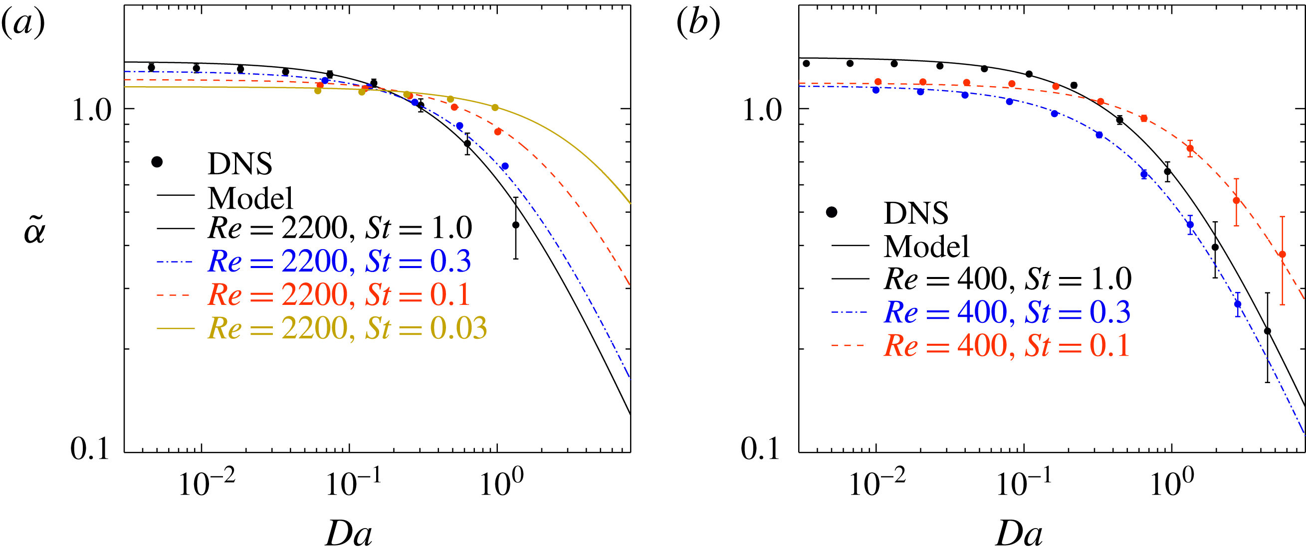
Normalized decay rate as a function of Damköhler number for different Stokes numbers. (a) The results for
 $Re=400$
(runs 2A–C), (b)
 $Re=2200$
(runs 3A–3D). Symbols represent simulation results, while lines correspond to the model given by (2.22). The values of
 $\unicode[STIX]{x1D6FC}_{c}$
, which are used in (2.22), can be found from table 1.

Figure 6 shows that by decreasing the Stokes number, the normalized reactant decay rate stays unchanged up to larger Damköhler numbers. This means that the effect of particle clustering is weaker for smaller Stokes numbers. This is expected since the limit of very small clusters corresponds to individual particles, where
 $\tilde{\unicode[STIX]{x1D6FC}}$
is independent of
 $Da$
.
If the turbulence is unchanged, a reduction in the Stokes number will, as is apparent from (3.9), yield a reduced relative velocity between the particles and the fluid. Based on (1.3), it is clear that this results in a decreased Sherwood number as long as the particle diameter is not changed while changing the Stokes number. This effect is identified in figure 6(b), where it is observed that the normalized reactant decay rate is monotonically decreasing with the Stokes number for small Damköhler numbers. (Please note that for small Damköhler numbers, the normalized reactant decay rate equals half of the Sherwood number.) The same monotonic decrease is, however, not observed for the cases with
 $Re=400$
, which is visualized in figure 6(a). This is because, as can be seen from table 1, for the
 $Re=400$
cases the particle diameter is smaller for
 $St=0.3$
than for
 $St=0.1$
, which happens to yield the same Sherwood number for
 $St=0.1$
and
 $St=0.3$
, and hence, the normalized reactant decay rates for small Damköhler numbers are equal.
Particle size is important, and in the following it is considered by the effects it has on the Sherwood number. From (2.23), it is clear that
 $$\begin{eqnarray}\displaystyle \tilde{\unicode[STIX]{x1D6FC}}=\overline{Sh}/2 & & \displaystyle\end{eqnarray}$$
for
 $Da\rightarrow 0$
. By inserting (2.11) and (3.9) into (1.3), the following expression for the mean particle Sherwood number is obtained:
 $$\begin{eqnarray}\displaystyle \overline{Sh}=2+0.69Sc^{1/3}\sqrt{\frac{u_{rms}\unicode[STIX]{x1D6FD}d_{p}}{\unicode[STIX]{x1D708}}}\left[\frac{Stk_{L}^{-2/3}-k_{\unicode[STIX]{x1D702}}^{-2/3}}{k_{L}^{1/3}-k_{\unicode[STIX]{x1D702}}^{-2/3}}\right]^{1/4}. & & \displaystyle\end{eqnarray}$$
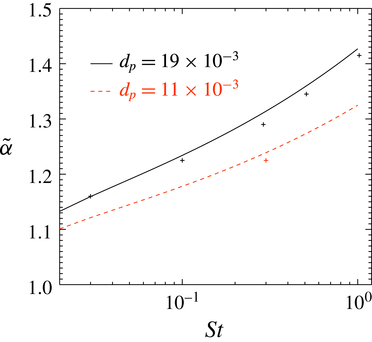
By combining the two equations above, one can now plot
 $\tilde{\unicode[STIX]{x1D6FC}}$
as a function of Stokes number for different particle diameters. This is done in figure 7, where the solid lines correspond to the expression discussed above and the symbols represent data from individual simulations with
 $Da=0.01$
. One can see from the figure that, except from a small downward shift, the simulation results follow the predictions. The reason for the downward shift is that the Damköhler number for the simulations is not infinitely small in reality, and hence the normalized decay rate is slightly smaller than it would have been for
 $Da\rightarrow 0$
.
Sherwood number as a function of Stokes number for
 $Re=400$
and
 $Da=0.01$
. Solid lines correspond to modelled results while symbols represent results from individual simulations.

3.4 The cluster decay rate
If the chemical time scale is much shorter than the lifetime of the particle clusters, the interior of the clusters will quickly be void of reactants. This means that the reactant consumption rate is controlled by the flux of reactant to the surface of the clusters, where the reactant will be consumed at the exterior of the cluster. Based on this, it is clear that for large
 $Da$
(small
 $\unicode[STIX]{x1D70F}_{c}$
), the clusters behave as large solid particles, or super-particles. Following Kruger et al. (Reference Kruger, Haugen, Løvas and Mitra2017), the reactant decay rate is then given by the so-called cluster decay rate:
 $$\begin{eqnarray}\displaystyle \unicode[STIX]{x1D6FC}_{c}=n_{c}\overline{\unicode[STIX]{x1D705}}_{c}\overline{A}_{c}, & & \displaystyle\end{eqnarray}$$
where
 $n_{c}=A_{1}\ell ^{-3}$
is the number density of clusters (or super-particles),
 $\overline{\unicode[STIX]{x1D705}}_{c}=D_{t}\overline{Sh}/\ell$
is the reactant diffusion rate to the super-particles,
 $\overline{A}_{c}=A_{2}\ell ^{2}$
is the surface area of the clusters,
 $D_{t}$
is the turbulent diffusivity that carries the reactant from the surrounding fluid to the surface of the clusters and
 $A_{1}$
and
 $A_{2}$
are constants that depend on the dimensionality of the clusters. It is clear that turbulent eddies larger than
 $\ell$
, as given by (3.11), cannot participate in the turbulent transport of reactants to the clusters, while eddies slightly smaller than
 $\ell$
will participate. A first approximation of the turbulent diffusivity to the surface of the clusters is therefore given by
 $$\begin{eqnarray}\displaystyle D_{t}=u_{\ell }\ell =u_{L}LSt^{2}. & & \displaystyle\end{eqnarray}$$
By combining the above, taking into account (3.11), it is found that
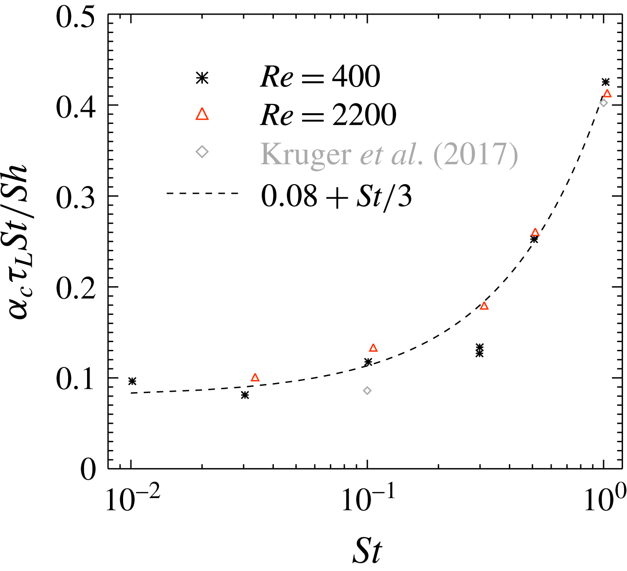
 $$\begin{eqnarray}\displaystyle \frac{\unicode[STIX]{x1D6FC}_{c}\unicode[STIX]{x1D70F}_{L}St}{\overline{Sh}}=A_{1}A_{2}, & & \displaystyle\end{eqnarray}$$
where the right-hand side should be constant for resonant eddies well inside the inertial range. From figure 8, it can be seen that the right-hand side of the above equation is constant only for Stokes numbers smaller than
 ${\sim}0.3$
. The values of the variables on the left-hand side of (3.17) are all found in table 1. Since the value of the right-hand side starts to increase already for
 $St=0.3$
, this may once again indicate that
 $\unicode[STIX]{x1D6FE}$
from (3.10) is different from unity. The discrepancy may also be due to the fact that when it comes to the shape of the particle clusters, a large scale strain may stretch them. For
 $St\sim 1$
, there are no vortices that are larger than the clusters, and hence the dimensionality of the clusters becomes different. This will inevitably yield different values of
 $A_{1}A_{2}$
. The value of the geometric coefficients can be fitted by
 $$\begin{eqnarray}\displaystyle A_{1}A_{2}=0.08+St/3, & & \displaystyle\end{eqnarray}$$
but this is just an empirical fit and more work is required in order to understand the fundamentals behind the shape and size of the particle clusters.
The product
 $\unicode[STIX]{x1D6FC}_{c}\unicode[STIX]{x1D70F}_{L}St$
as a function of
 $St$
for runs with resonant eddies in the inertial range. Symbols represent simulation results, while the line corresponds to the model given by (3.18). The points labelled ‘Kruger’ correspond to results obtained from data found in Kruger et al. (Reference Kruger, Haugen, Løvas and Mitra2017), where the Sherwood number was set to 2 and the Reynolds number was 250.

In figure 8, it can be seen that the two points for
 $St=0.3$
and
 $Re=400$
are very close together. Since these two simulations had different particle sizes, the fact that they yield essentially the same value of
 $A_{1}A_{2}$
supports the assumption that the expression for
 $A_{1}A_{2}$
, as shown in (3.18), is independent on particle size.
4 Conclusion
In this work, the effect of turbulence on the mass (and heat) transfer between inertial particles and the embedding fluid is studied. The turbulence is shown to have two effects on the mass transfer. The first effect is active for all Damköhler numbers, and here the turbulence increases the mass transfer rate due to the relative velocity between the particles and the fluid. A corresponding model for the relative velocity between the fluid and the particles is given by (3.9), which uses basic variables of the flow. This model is the first main result of this paper. With this, adding effects of relative velocity into RANS based simulations is straightforward.
The second effect with which turbulence influences the mass transfer rate is through the clustering of particles. It is shown in §§ 3.2 and 3.3 that the size of the particle clusters increases with the particle Stokes number, and that the clustering decreases the overall mass transfer rate between the particles and the fluid. It is also clear that the effect of clustering is strong, and a reduction in reactant decay by a factor of 10 is seen already for Damköhler numbers of the order of 10. This is a confirmation of the findings of Kruger et al. (Reference Kruger, Haugen, Løvas and Mitra2017). For many applications, it may therefore lead to critically large errors if the effect turbulent clustering of particles has on the reaction rate is neglected. In the current work, a model has been developed that takes this effect into account and incorporates it into a modified Sherwood number. This is done by combining (2.22) and (2.23) with (3.17), such that the modified Sherwood number becomes
 $$\begin{eqnarray}\displaystyle Sh_{mod}=\overline{Sh}\frac{A_{1}A_{2}}{A_{1}A_{2}+DaSt/2}, & & \displaystyle\end{eqnarray}$$
where
 $A_{1}A_{2}$
is given by (3.18). The above equation should be used, together with e.g. (2.24) and (2.25), to obtain the correct mass transfer rate to the particles in standard RANS simulation tools. This is the second main result of this paper.
More work is still required in order to fully understand the size and dimensionality of the particle clusters. As of now, a unique way of characterizing particle clusters does not exist, and very little work has actually been put into the study of large scale clustering of particles.
The work presented here is related to mono-disperse particles. Since particles of different Stokes numbers will cluster in different regions of the flow, one may expect that the effect of particle clustering on the reactant decay rate is reduced for very broad particle size distributions. This should be studied in future work.
Acknowledgements
The research leading to these results has received funding from the Polish-Norwegian Research Program operated by the National Centre for Research and Development under the Norwegian Financial Mechanism 2009-2014 in the frame of Project Contract No. Pol-Nor/232738/101/2014. The Research project ‘Gaspro’, financed by the research council of Norway (267916), has also contributed to this research. This work was supported by the grant ‘Bottlenecks for particle growth in turbulent aerosols’ from the Knut and Alice Wallenberg Foundation, no. KAW 2014.0048, and by a grant from the Swedish Research Council (no. 638-2013-9243). N.E.L.H. and D.M. also acknowledge the Research Council of Norway under the FRINATEK grant 231444.