2.1. Governing equations

The flow of the film is governed by the incompressible, axisymmetric Navier–Stokes equations:

(2.1a)\begin{gather} \bar{\rho}(\bar{u}_{\bar{t}}+\bar{u}\bar{u}_{\bar{r}}+\bar{w}\bar{u}_{\bar{z}})={-}\bar{p}_{\bar{r}}+\bar{\mu}\left[\frac{1}{\bar{r}}\partial_{\bar{r}}(\bar{r}\bar{u}_{\bar{r}})+\bar{u}_{\bar{z}\bar{z}}-\frac{\bar{u}}{\bar{r}^2}\right], \end{gather}

(2.1b)\begin{gather}\bar{\rho}(\bar{w}_{\bar{t}}+\bar{u}\bar{w}_{\bar{r}}+\bar{w}\bar{w}_{\bar{z}})={-}\bar{p}_{\bar{z}}+\bar{\mu}\left[\frac{1}{\bar{r}}\partial_{\bar{r}}(\bar{r}\bar{w}_{\bar{r}})+\bar{w}_{\overline{zz}}\right]-\bar{\rho}\bar{g}, \end{gather}

(2.1c)\begin{gather}\frac{1}{\bar{r}}\partial_{\bar{r}}(\bar{r}\bar{u})+\bar{w}_{\bar{z}}=0, \end{gather}

where $(\bar {u},\bar {w})$ denote velocity in the radial, $\bar {r}$, and axial, $\bar {z}$, directions respectively, with $\bar {z}$ increasing in the upward direction along the tube. Other variables and parameters include pressure $\bar {p}$, density $\bar {\rho }$, viscosity $\bar {\mu }$ and acceleration due to gravity $\bar {g}$. Figure 1 shows a schematic of the tube and the variables; additional variables include $\bar {R}_0$ denoting the average distance from the tube centre $\bar {r}=0$ to the film's free surface, and $\bar {R}(\bar {z},\bar {t})$ denoting the distance from the tube centre to the free surface. The radius of the tube is given by $\bar {a}$ and $\bar {\kappa }$ is a typical length scale in the axial direction, such as a wavelength of a typical disturbance. Quantities with dimensions are denoted with an overbar, and subscripts denote partial derivatives.

Figure 1.

Schematic diagram of the rigid tube set-up and definition of variables.

Typically a no-slip boundary condition is applied at the tube wall $\bar {r}=\bar {a}$. Here, we investigate the effects of slip on the film flow with a Navier slip boundary condition with slip length $\bar {\varLambda }$:

(2.2a)\begin{gather} \bar{w}={-}\bar{\varLambda}\, \bar{w}_{\bar{r}}, \end{gather}

(2.2b)\begin{gather}\bar{u}=0. \end{gather}

We note that boundary condition (2.2a) also arises in the study of flow of a film along a porous tube wall since, under certain simplifying assumptions, the flow of the film decouples from the flow within the pores. Briefly, the axial velocity in the porous medium, governed by Darcy's law, is given by $\bar {w}^{(m)}=-\bar {K}(\bar {p}_{\bar {z}}-\bar {\rho } \bar {g})/\bar {\mu }$, where $\bar {K}$ is the permeability. Permeability values for natural materials vary widely. Typical values for soils are between $10^{-9}$ and $10^{-10}$ whereas for clean gravel they are between $10^{-7}$ and $10^{-9}$. At the fluid–porous wall interface, the Beavers–Joseph boundary condition $\bar {w}_{\bar {r}}=-\bar {\alpha }(\bar {w}-\bar {w}^{(m)})/\sqrt {\bar {K}}$ may be used for the axial velocity (Beavers & Joseph Reference Beavers and Joseph1967), where $\alpha$ is a parameter with value determined by the properties of the porous medium. If the pore velocity $\bar {w}^{(m)}$ is much smaller than the film velocity $\bar {w}$, a condition that holds if $\bar {K}/\bar {h}_0^2\ll 1$, where $\bar {h}_0$ is the mean film thickness, then this boundary condition may be approximated by (2.2a); see, for example, Pascal (Reference Pascal1999) and Liu & Ding (Reference Liu and Ding2017) and references therein for further discussion.

At the free surface $\bar {r}=\bar {R}(\bar {z},\bar {t})$ we require continuity of tangential stress:

(2.3)\begin{equation} (\bar{w}_{\bar{r}}+\bar{u}_{\bar{z}})(1-\bar{R}^2_{\bar{z}})+2(\bar{u}_{\bar{r}}-\bar{w}_{\bar{z}})\bar{R}_{\bar{z}}=\bar{\tau}^{(g)}, \end{equation}

with $\bar {\tau }^{(g)}$ denoting the tangential stress exerted by the gas flow on the film's free surface; a jump in normal stress (according to the Young–Laplace law):

(2.4)\begin{align} &2\bar{\mu}(\bar{u}_{\bar{r}}+\bar{w}_{\bar{z}}\bar{R}^2_{\bar{z}})+\bar{\mu}\bar{R}_{\bar{z}}(\bar{w}_{\bar{r}}+\bar{u}_{\bar{z}})-2\bar{\mu}^{(g)}(\bar{u}_{\bar{r}}^{(g)}+\bar{w}_{\bar{z}}^{(g)}\bar{R}^2_{\bar{z}})-\bar{\mu}^{(g)}\bar{R}_{\bar{z}}(\bar{w}^{(g)}_{\bar{r}}+\bar{u}^{(g)}_{\bar{z}}) \nonumber\\ &\quad = (\bar{p}-\bar{p}^{(g)})(1+\bar{R}_{\bar{z}}^2)+\bar{\sigma}(1+\bar{R}^2_{\bar{z}}) \left(\frac{1}{\bar{R}(1+\bar{R}^2_{\bar{z}})^{1/2}}-\frac{\bar{R}_{\overline{zz}}}{(1+\bar{R}^2_{\bar{z}})^{3/2}}\right), \end{align}

with $\bar {\sigma }$ the surface tension and superscripts of $(g)$ denoting variables in the core gas flow; and the kinematic condition

(2.5)\begin{equation} \bar{u}=\bar{R}_{\bar{t}}+\bar{w}\bar{R}_{\bar{z}}. \end{equation}

There is a steady ‘flat-film’ solution to (2.1)–(2.5) with $\bar {w}=\bar {w}(\bar {r})$, $\bar {p}=\bar {p}(\bar {z})$, $\bar {u}=0$ and with free surface $\bar {R}=\bar {R}_0$:

(2.6)\begin{align} \bar{w}=\frac{1}{4}\left(\frac{\bar{p}_{\bar{z}}^{(g)}+\bar{\rho}\bar{g}}{\bar{\mu}}\right)\left(\bar{r}^2-\bar{a}^2-2\bar{R}_0^2\ln\frac{\bar{r}}{\bar{a}}-\frac{2\bar{\varLambda}}{\bar{a}}(\bar{a}^2-\bar{R}_0^2)\right)+\bar{R}_0\bar{\tau}^{(g)}\left(\ln\frac{\bar{r}}{\bar{a}}-\frac{\bar{\varLambda}}{\bar{a}}\right). \end{align}

In the no-slip limit, i.e. $\bar {\varLambda }=0$, the velocity profile takes on the form seen in, for example, Camassa & Ogrosky (Reference Camassa and Ogrosky2015). As this solution is unstable to long-wave disturbances, long-wave asymptotics will be used to derive a model for the evolution of the free surface next.

2.2. Model derivation

Equations (2.1)–(2.5) may be made dimensionless using the following reference scales:

(2.7a–g)\begin{align} r=\frac{\bar{r}}{\bar{R}_0}, \quad z=\frac{\bar{z}}{\bar{\kappa}}, \quad u=\frac{\bar{u}}{\bar{U}_0}, \quad w=\frac{\bar{w}}{\bar{W}_0}, \quad t=\frac{\bar{t}\bar{W}_0}{\bar{\kappa}}, \quad p=\frac{\epsilon\bar{p}{\bar{R}_0}}{\bar{\mu}\bar{W}_0}, \quad \tau=\frac{\bar{\tau}\bar{R}_0}{\bar{\mu}\bar{W}_0}, \end{align}

where $\bar {U}_0$ and $\bar {W}_0$ are reference velocity scales. Since we will be considering airflow moving up the tube at a constant volume flux due to an imposed pressure gradient, here we use the mean centreline velocity of the air for the axial velocity scale:

(2.8)\begin{equation} \bar{W}_0=\frac{2\bar{Q}^{(g)}}{{\rm \pi} \bar{R}_0^2}, \end{equation}

where $\bar {Q}^{(g)}$ is the (constant) volume flux of air. This choice of scales is similar to that used by Camassa et al. (Reference Camassa, Forest, Lee, Ogrosky and Olander2012). In the following model derivation, the ‘long-wave’ assumption,

(2.9)\begin{equation} \epsilon=\frac{\bar{R}_0}{\bar{\kappa}}\ll 1, \end{equation}

is made. Using the relation (2.9), we also obtain that $\bar {U}_0=\epsilon \bar {W}_0$ due to the continuity equation (2.1c). The exact value of the length scale $\bar {\kappa }$, which denotes a typical free-surface wavelength, need not necessarily be specified when deriving the model (though this value could be taken to be one of several reasonable choices, including (i) the most unstable wavelength, $2\sqrt {2}{\rm \pi} \bar {R}_0$, arising due to the Plateau–Rayleigh instability as found in § 3, or (ii) the typical wavelength of a travelling wave seen in simulations). Note that while other length-scale ratios could be employed in the asymptotic expansion, the ratio of $\bar {R}_0/\bar {\kappa }$ is a natural one to use due to the dependence of the most unstable free-surface wavelength on the mean free-surface radius $\bar {R}_0$.

Substituting (2.7a–g) into (2.1)–(2.5) results in

(2.10a)\begin{gather} \epsilon^3 Re(u_t+uu_r+wu_z)={-}p_r+\epsilon^2\left[\frac{1}{r}\partial_r(ru_r)+\epsilon^2 u_{zz}+\frac{u}{r^2}\right], \end{gather}

(2.10b)\begin{gather}\epsilon Re(w_t+uw_r+ww_z)={-}p_z+\left(\frac{1}{r}\partial_r(rw_r)+\epsilon^2w_{zz}\right)-\frac{Re}{Fr^2}, \end{gather}

(2.10c)\begin{gather}\frac{1}{r}\partial_r(ru)+w_z=0, \end{gather}

where $Re=\bar {\rho }\bar {W}_0\bar {R}_0/\bar {\mu }$ and $Fr=\bar {W}_0/\sqrt {\bar {g}\bar {R}_0}$ are the Reynolds and Froude numbers, respectively.

The boundary conditions at the wall $r=a$ are

(2.11a,b)\begin{equation} w={-}\varLambda w_r,\quad u=0.\end{equation}

The boundary conditions at the free surface $r=R(z,t)$ are given by

(2.12a)\begin{equation} (w_r+\epsilon^2u_z)(1+\epsilon^2R_z^2)+2\epsilon^2(u_r+w_z)R_z=\tau^{(g)},\\ \end{equation}

(2.12b)\begin{align} &2\epsilon(u_r+\epsilon^2w_z R_z^2)+\epsilon R_z(w_r+\epsilon^2 u_z)-2\epsilon(u_r^{(g)}+\epsilon^2w_z^{(g)} R_z^2)-\epsilon R_z(w_r^{(g)}+\epsilon^2 u_z^{(g)})\nonumber\\ &\quad=(1+\epsilon^2R_z^2)\left[\frac{p-p^{(g)}}{\epsilon} +\frac{1}{C}\left(\frac{1}{R(1+\epsilon^2 R_z^2)^{1/2}}-\frac{\epsilon^2 R_{zz}}{ (1+\epsilon^2 R_z^2)^{3/2}}\right)\right], \end{align}

(2.12c)\begin{equation} u=R_t+wR_z, \end{equation}

where ${C}=\bar {\mu }\bar {W}_0/\bar {\sigma }$ is the capillary number.

In the limit $\epsilon \to 0$, the governing equations become

(2.13a)\begin{gather} 0=p_r, \end{gather}

(2.13b)\begin{gather}\frac{1}{r}(\partial_r(rw_r))=p_z+\frac{Re}{Fr^2}, \end{gather}

(2.13c)\begin{gather}\frac{1}{r}\partial_r(ru)+w_z=0, \end{gather}

while the boundary conditions at the free surface $r=R(z,t)$ are

(2.14a)\begin{gather} w_r=\tau^{(g)}, \end{gather}

(2.14b)\begin{gather}-p={-}p^{(g)}+\frac{\epsilon}{C}\left(\frac{1}{R}-\epsilon^2R_{zz}\right), \end{gather}

(2.14c)\begin{gather}u=R_t+wR_z. \end{gather}

While the surface tension terms in (2.14b) do not appear strictly at leading order, they are retained as in numerous other modelling studies of such film flows. These terms have been shown in previous studies to accurately capture the upper bound on unstable wavenumbers, and the second term has been demonstrated to be the lowest-order one that prevents shock formation. For flows down an inclined plane with high surface tension and low volume flux, Gjevik (Reference Gjevik1970) explored the role of these terms in the saturation of instability growth and identified their impact on the phase speed and amplitude of free-surface waves of finite amplitude.

Our model equation for the evolution of the film's free surface may be found by integrating (2.13c) across the fluid layer to obtain

(2.15)\begin{equation} R_t-\frac{1}{R}\frac{\partial}{\partial z}\int_R^a wr\,{\rm d}r=0. \end{equation}

In order to produce a closed model, an approximate expression is needed for $w$. This may be found by solving (2.13b) for $w$ by integrating twice and making use of the boundary conditions (2.11a,b) and (2.14a) to get

(2.16)\begin{equation} w=\frac{1}{4}\left(p_z+\frac{Re}{Fr^2}\right)(r^2-a^2-2\tilde{\varLambda} a^2)+\left(R\tau^{(g)}- \frac{R^2}{2}\left(p_z+\frac{Re}{Fr^2}\right)\right)\left(\ln \left(\frac{r}{a}\right)- \tilde{\varLambda}\right),\end{equation}

where $\tilde {\varLambda }=\varLambda /a$ is a rescaled slip length.

Next, estimates for the stresses $\tau ^{(g)}$ and $p_z^{(g)}$ imparted by the air at the free surface are needed. There are many options for estimating these stresses; here, we use the ‘locally Poiseuille’ approach of Camassa et al. (Reference Camassa, Forest, Lee, Ogrosky and Olander2012) in which a laminar profile for the core flow is assumed. This approach has the advantage of providing an extremely simple estimate of the stresses with the drawback that these estimates have been shown to be underestimates in some experiments with turbulent airflow (though a modified effective viscosity can mitigate these issues; see e.g. Camassa et al. (Reference Camassa, Forest, Lee, Ogrosky and Olander2012) for details). Other options which may be more appropriate for turbulent airflow include those of Trifonov (Reference Trifonov2010), Tseluiko & Kalliadasis (Reference Tseluiko and Kalliadasis2011) and Camassa et al. (Reference Camassa, Ogrosky and Olander2017); incorporating these closures into this model with slip is left for future work.

In this ‘locally Poiseuille’ approach, the free-surface variations are assumed to be slowly varying in the axial direction, consistent with the long-wave derivation used above. The core flow is modelled with the simple laminar profile of Poiseuille flow through a pipe, with the free surface, slowly varying in $z$, serving as the air's ‘tube wall’ here. A brief derivation is now given. The air is assumed to flow at a constant volume flux $\bar {Q}^{(g)}$:

(2.17)\begin{equation} \bar{Q}^{(g)}=\int_0^{\bar{R}} 2{\rm \pi} \bar{r}\bar{w}^{(g)}\,{\rm d}\bar{r}.\end{equation}

The velocity profile $\bar {w}^{(g)}(\bar {r})$ for $0<\bar {r}<\bar {R}(\bar {z},\bar {t})$ is estimated by a slowly varying Poiseuille flow profile with zero velocity at the free surface $\bar {r}=\bar {R}(\bar {z},\bar {t})$:

(2.18)\begin{equation} \bar{w}^{(g)}=\frac{\bar{p}_{\bar{z}}^{(g)}}{4\bar{\mu}^{(g)}}(\bar{r}^2-\bar{R}^2).\end{equation}

Substituting (2.18) into (2.17), integrating and solving for $\bar {p}_{\bar {z}}^{(g)}$ gives an estimate of the gas pressure gradient:

(2.19)\begin{equation} \bar{p}_{\bar{z}}^{(g)}={-}\frac{8\bar{\mu}^{(g)}\bar{Q}^{(g)}}{{\rm \pi} \bar{R}^4}. \end{equation}

Similarly, the tangential stress applied by the core flow on the free surface may be estimated by evaluating $\bar {\mu }^{(g)}\bar {w}_{\bar {r}}$ at the free surface $\bar {r}=\bar {R}(\bar {z},\bar {t})$:

(2.20)\begin{equation} \bar{\tau}^{(g)}=\frac{4\bar{Q}^{(g)}}{{\rm \pi}\bar{R}^3}.\end{equation}

In dimensionless form, and after substituting (2.19) and (2.20) into (2.14a) and (2.14b), respectively, we get the estimates needed to close the model:

(2.21a,b)\begin{equation} p_z={-}\frac{4}{mR^4}+\frac{\varepsilon}{\mathrm{C}R^2}(R_z+\varepsilon^2 R^2R_{zzz}) \quad \text{and} \quad \tau^g ={-}\frac{2}{mR^3}, \end{equation}

where $m=\bar {\mu }/\bar {\mu }^{(g)}$. Plugging these stresses into the velocity results in the final model equation:

(2.22)\begin{equation} {R_t+[S_1\,f_1(R,a)+S_2\,f_2(R,a)]R_z+\frac{S_3}{R}[f_3(R,a)(R_z+R^2R_{zzz})]_z}=0,\end{equation}

where

(2.23a–c)\begin{equation} S_1=\frac{1}{m}, \quad S_2=\frac{Re}{2Fr^2}, \quad S_3=\frac{1}{16{C}}, \end{equation}

and where

(2.24a)\begin{gather} {f_1(R,a)}=\frac{a^2}{R^4}\left[\frac{a^2}{R^2}-1+2\tilde{\varLambda}\left(\frac{2a^2}{R^2}-1\right)\right], \end{gather}

(2.24b)\begin{gather}{f_2(R;a)}=R^2-a^2+2R^2\ln\left(\frac{a}{R}\right)-2\tilde{\varLambda}(a^2-R^2), \end{gather}

(2.24c)\begin{gather}{f_3(R,a)}=\frac{a^4}{R^2}+3R^2-4a^2+4R^2\ln\left(\frac{a}{R}\right)+\frac{4\tilde{\varLambda}}{R^2}(a^2-R^2)^2. \end{gather}

The notation adopted here is similar to that used by Camassa et al. (Reference Camassa, Forest, Lee, Ogrosky and Olander2012) to provide ease of comparison. The $S_1$ term represents the effects of core flow acting through the free-surface stresses, while the $S_2$ term contains the effect of gravity acting on the film. The $S_3$ terms contain the effects of surface tension acting at the free surface. Equation (2.22), a conservation law for $R^2$, conserves fluid volume. As in Camassa et al. (Reference Camassa, Forest, Lee, Ogrosky and Olander2012), here $z$ and $t$ are rescaled by $\epsilon$ in order to return to the original aspect ratio. As a result, $\epsilon$ is scaled out of (2.22), but the validity of the derivation still relies on the assumption $\epsilon \ll 1$.

If $S_1=0$, the model is identical to the one derived by Liu & Ding (Reference Liu and Ding2017) for film flow over a porous wall. In the no-slip limit, i.e. $\tilde {\varLambda }=0$, the model of Camassa et al. (Reference Camassa, Forest, Lee, Ogrosky and Olander2012) is recovered; furthermore, if $\tilde {\varLambda }=0$ and $S_1=0$ the no-slip falling-film model of Camassa et al. (Reference Camassa, Ogrosky and Olander2014) is recovered. (There is a slight difference in the definition of $S_2$ here and in Camassa et al. (Reference Camassa, Ogrosky and Olander2014) due to having neglected the density of the core fluid – taken here to be air – in the current derivation.) Note that for a falling film, time may be rescaled by $S_2$ and the dynamics is governed by the single parameter ratio $S_3/S_2$. Finally, if $\tilde {\varLambda }=0$, $S_2=0$ and $S_1\ne 0$, the no-slip model of Camassa & Ogrosky (Reference Camassa and Ogrosky2015) is recovered; in this case, time may be rescaled by $S_1$ with the dynamics governed by $S_3/S_1$.

We note that for the falling-film case with passive core ($S_1=0, S_2>0$) it would be appropriate to derive the model equation using a different velocity scale (e.g. the Nusselt velocity $\bar {W}_N=\bar {\rho } \bar {g} \bar {h}_0^2/\bar {\mu }$) from the core flow scale of (2.8), as done in Camassa et al. (Reference Camassa, Ogrosky and Olander2014) and Liu & Ding (Reference Liu and Ding2017) for the no-slip and slip cases, respectively. As the resulting model equation, however, is identical in form to those of (2.22), a separate derivation is omitted here.

2.3. Thin-film limit

If the film thickness is assumed to be small relative to the tube radius, the model may be simplified. Defining a rescaled film thickness

(2.25)\begin{equation} \eta=\frac{a-R}{a-1}, \end{equation}

so that $\eta =0$ at the wall and $\eta =1$ at the undisturbed free surface $r=R_0$, substituting $R=a-\beta \eta$, where $\beta =a-1$, into (2.22) and expanding about $\beta =0$ results in

(2.26)\begin{align} &\eta_t+2\beta S_1\left[(\eta+\varLambda^*)+\beta\left(\frac{11}{2}\eta^2+8\varLambda^*\right)\right]\eta_z-2\beta^2S_2(\eta^2+2\varLambda^*\eta)\eta_z \nonumber\\ &\quad +\frac{16\beta^3S_3}{3}[(\eta^3+3\varLambda^*\eta^2)(\eta_z+\eta_{zzz})]_z=0. \end{align}

Here $\varLambda ^*=\varLambda /\beta$ is a rescaled slip length, and terms up to $O(\beta ^2)$ have been retained in both the $S_1$ and $S_2$ terms, while terms of $O(\beta ^3)$ have been retained in the $S_3$ terms. Several models previously reported in the literature can be recovered in various limits. In the no-slip limit with $\varLambda ^*=0$, the thin-film model of Camassa & Ogrosky (Reference Camassa and Ogrosky2015) is recovered; if, in addition, $S_1=0$, the model of Frenkel (Reference Frenkel1992) is recovered while if $S_2=0$, the model of Kerchman (Reference Kerchman1995) is recovered. In the absence of any base flow, i.e. $S_1=S_2=0$ and $\tilde {\varLambda }=0$, then the model of Hammond (Reference Hammond1983) is recovered. In the case of slip where $\varLambda ^*>0$, if $S_1=0$, the model reduces to that derived by Halpern & Wei (Reference Halpern and Wei2017) for flow down a fibre.

Note that the $S_1$ term appears at $O(\beta )$ while the $S_2$ term appears at $O(\beta ^2)$. We also note that (2.26) is a conservation law for film thickness $h$ while (2.22) is a conservation law for fluid volume. Note that in the thin-film limit $h/a\rightarrow 0$, conserving $h$ and conserving $R^2$ are identical; for moderately thick films, however, approximating fluid volume conservation can lead to distinct behaviour in model solutions (e.g. Camassa & Ogrosky Reference Camassa and Ogrosky2015).

2.4. Parameter values

Before finding model solutions, we briefly discuss parameter values that are relevant for experiments from the literature. First, it should be emphasized that terms of $O(\epsilon Re)$ have been assumed small in the derivation here. This model is thus only applicable in situations where the Plateau–Rayleigh instability may be expected to dominate the Kapitza instability. For higher-Reynolds-number flows, one might opt to retain the inertial terms in the derivation, or use an integral boundary layer modelling approach, which has been shown to have success matching experiments with moderate to high liquid Reynolds number.

Second, relevant values of slip length parameter $\varLambda$ are discussed. For liquid flows over rough surfaces without any superhydrophobic properties, slip lengths are typically of the order of hundreds of nanometres. These slip lengths may be larger for flows involving polymeric liquids like silicone oil; such liquids have been shown to produce an apparent wall slip length of $1\unicode{x2013}10\ \mathrm {\mu }{\rm m}$ (Brochard-Wyart et al. Reference Brochard-Wyart, de Gennes, Hervert and Redon1994). Thus, for example, for films inside tubes with mean free surface $\bar {R}_0$ of the order of 1 mm ($10\ \mathrm {\mu }{\rm m}$), one may have $\varLambda \approx 0.001$ (0.1). Slip lengths within this range may be expected in some of the falling-film experiments conducted by Camassa et al. (Reference Camassa, Ogrosky and Olander2014) using silicone oil inside tubes of radius $\bar {a}=0.5$, 0.295 and 0.17 cm; the smallest tube had films with mean free surface $\bar {R}_0 = 0.5$–1.2 mm, resulting in $\varLambda$ taking on values as large as 0.01. The experiments of Camassa et al. (Reference Camassa, Forest, Lee, Ogrosky and Olander2012) consider a silicone oil film driven up a tube by airflow with $\bar {R}_0\approx 0.4$ cm, resulting in $\varLambda$ taking on values of the order of 0.001. For flow over hydrophobic surfaces or over a porous medium, larger values of slip length may be appropriate, as discussed in related studies; for example, Liu & Ding (Reference Liu and Ding2017) consider a falling film with dimensionless slip lengths that, in the scaling used here, correspond to $\varLambda \approx 0.1$. For film flows outside of a tube, Halpern & Wei (Reference Halpern and Wei2017) have shown that inclusion of slip in a falling-film model can account for discrepancies between no-slip models and the experiments of Quéré (Reference Quéré1990) on falling films and droplets along fibres; in these experiments, the film thickness was as small as $20\ \mathrm {\mu }{\rm m}$. With these applications in mind, we present results for values of $\tilde {\varLambda }$ primarily covering a range of values from a few thousandths to a tenth. In a few instances results are also presented for larger values of $\tilde {\varLambda }$ in order to explore the mathematics of the model at larger slip lengths.

Third, the values of $S_1$, $S_2$ and $S_3$ used here were chosen to be compatible with previous experiments. In the falling-film experiments of Camassa et al. (Reference Camassa, Ogrosky and Olander2014), the silicone oil used had viscosity $\bar {\mu }=129$ P, density $\rho =0.97\ {\rm g}\ {\rm cm}^{-3}$ and surface tension $\gamma =21.5\ {\rm dyn}\ {\rm cm}^{-1}$, corresponding to a Kapitza number $Ka=3.3\times 10^{-3}$. For experiments with $\bar {a}=0.295$ cm, this results in the ratio $S_3/S_2$ taking on values in the range 0.05–0.8; for $\bar {a}=0.17$ cm, the ratio $S_3/S_2$ takes on values in the range 0.2–1.1. 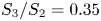Results are presented below for $S_3/S_2=0.35$ which fall within both of these ranges. The value of $a$ in these smaller-radius experiments took on a wide range of values, from 1.28 to 6. In the air-driven experiments of Camassa et al. (Reference Camassa, Forest, Lee, Ogrosky and Olander2012), which used silicone oil with the same density, viscosity and surface tension as those of Camassa et al. (Reference Camassa, Ogrosky and Olander2014), $\bar {a}=0.5$ cm, the volume flux of air $Q^{(g)}$ ranged from 330 to $1170\ {\rm cm}^3\ {\rm s}^{-1}$ and $\bar {R}_0$ took on values from 0.35 to 0.45 cm. The value of $a=\bar {a}/\bar {R}_0$ ranged from 1.1 to 1.45. The ratio $S_2/S_1$ used in the no-slip model to compare with these experiments covered a range of values from 1 to near 100, with this range partly dependent on whether a modified effective viscosity is used as a model for the effects of airflow turbulence; while admittedly crude, this approach was shown to qualitatively capture features of the experiments. The ratio $S_3/S_1$, which may be expected to govern the dynamics for strong airflow, took on values of 0.01–1.

Here, results are presented with $S_2/S_1=8$ which with $a=2$ corresponds to $Re^{(g)}=3700$ and $Re^{(l)}=\bar {\rho }\bar {W}_N\bar {R}_0/\bar {\mu }=8.7\times 10^{-4}$. These values could be realized, for example, in the experiments of Camassa et al. (Reference Camassa, Forest, Lee, Ogrosky and Olander2012) with tube radius $\bar {a}=0.5$ cm, air volume flux $\bar {Q}^{(g)}=670\ {\rm cm}^3\ {\rm s}^{-1}$, an effective viscosity $\bar {\mu }^{(g)}=5.4\times 10^{-4}\ {\rm g}\ {\rm cm}^{-3}$ and mean free-surface radius $\bar {R}_0=0.25$ cm, resulting in $S_3/S_1=0.36$. For falling films, results are presented with $S_3/S_2=0.35$, which with $a=1.9$ corresponds to $Re^{(l)}=2.8\times 10^{-5}$. These values correspond to the smallest-tube-radius experiments of Camassa et al. (Reference Camassa, Ogrosky and Olander2014) with $\bar {a}=0.17$ cm and $\bar {R}_0=0.09$ cm.

4.1. Transient solutions

Equation (2.22) may be solved approximately using the method of lines; a brief outline is given here, with more details available elsewhere (e.g. Camassa et al. Reference Camassa, Ogrosky and Olander2014). Periodic boundary conditions in $z$ were used. The initial condition consisted of a constant free surface $R_0$ perturbed by one or more small-amplitude Fourier modes. A variety of wavenumbers, amplitudes and phase shifts were used. For the most part, the results were independent of initial conditions used; one exception is that there is a range of unperturbed film thickness for which the occurrence and timing of plug formation may depend on the initial conditions. This dependence, however, only occurs over a small range and further exploration of this sensitivity is left for future work.

The algorithm used is pseudospectral with spatial derivatives being calculated in Fourier space while nonlinear terms are calculated in physical space. To integrate with respect to time, a second-order predictor–corrector scheme is used. The strongly nonlinear terms required that the Fourier coefficients be dealiased after every time step. The total volume of fluid was monitored during the simulation; if this value varied more than some small specified tolerance, the simulation was rerun with smaller $\Delta z$ and $\Delta t$. These numerical solutions were verified by comparing instability growth and propagation early in simulations with the linear stability analysis results and with no-slip results from earlier studies.

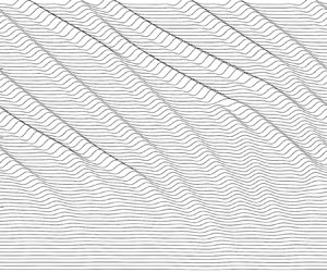
The case of passive core flow ($S_1=0$) is considered first. Figure 6 shows successive snapshots of the free surface taken at regularly spaced time intervals from numerical solutions to (2.22). In order to track the wave crests properly, each snapshot has been aligned by shifting it in $z$ by an amount corresponding to the phase speed found in § 3 (or approximately the phase speed, due to the discretization used when numerically finding solutions). It is worth noting that gravity is acting from right to left in these plots; hence, the waves are moving in the negative $z$ direction. In each of the simulations shown, $S_1=0$, $S_3/S_2=0.35$ and $a=1.27$ (here $S_2=1.607$, $S_3=0.568$, though the specific values do not affect the dynamical outcomes, only the time scale of the evolution). In the absence of pressure-driven airflow, the film flows down the tube. During the early stages, waves grow in amplitude with the expected growth rate; at later stages, one of two things happen. For small values of $\tilde {\varLambda }$, the nonlinearities in the model cause the saturation of wave growth, resulting in wave trains propagating down the tube; these waves interact with one another, but maintain a mostly steady shape.

Figure 6.

(a–c) Time snapshots showing the evolution of the free surface for (2.22) in a periodic domain with $S_1=0$, $S_3/S_2=0.35$ and $a=1.25$: (a) $\tilde {\varLambda }=0$, (b) $\tilde {\varLambda }=0.015$ and (c) $\tilde {\varLambda }=0.07$. The free-surface profiles are shown for equal time intervals. Profiles are shown in a frame of reference moving with the phase speed according to (3.7). (d–f) Time snapshots at the end of the simulations shown in (a–c), respectively; snapshots are shown inside a tube. For (f), snapshot shown occurs just after the final snapshot in (c). (g) Plots of $\max _zh(z,t)$ and $\min _zh(z,t)$ for simulations in (a–c). Waves flowing down the tube due to gravity are moving in the negative $z$ direction.

For larger values of $\tilde {\varLambda }$, the fastest-growing wave may undergo accelerated growth, with the wave crest appearing to approach the centre of the tube in finite time. This $R\rightarrow 0$ behaviour is an indication of plug formation and may be taken as a model prediction that plugs will form. This same behaviour can also occur due to the merger of two free-surface waves as occurs in figure 6(c) near the right of the final snapshot shown. In order to see the amplitude of these waves during the late-time stages of each simulation more clearly, figures 6(d)–6(f) show the free surface in the tube geometry at the final time of each simulation shown in figures 6(a)–6(c), respectively. In order to show the free surface as close to plug formation as possible, the free surface shown in figure 6(f) corresponds to the simulation shown in figure 6(c) but at $t=370.74$, which is just past the final time shown in figure 6(c). We note that the model solution cannot be continued all the way to $R=0$ due to the inverse powers and logarithms of $R$ in (2.22); it is also likely that the simplifying assumptions used in deriving the model (e.g. negligible inertia) may not be satisfied during the latter stages of plug formation. The maximum and minimum film thickness for each simulation is shown in figure 6(g). The accelerated growth for $\tilde {\varLambda }=0.07$ as $\min R\rightarrow 0$ in finite time is clearly seen.

There appears to be a critical value of $\tilde {\varLambda }$ above which plug formation occurs. It is likewise the case that, for fixed $\tilde {\varLambda }$, there is a critical value of film thickness parameter $a$ above which plug formation occurs, as has been shown for the no-slip limit of (2.22) in Camassa et al. (Reference Camassa, Ogrosky and Olander2014) (similarly, for fixed $a$, increasing the $S_3/S_2$ ratio past a critical value promotes plug formation as in Ogrosky (Reference Ogrosky2021b)). Thus it appears that in the absence of pressure-driven flow, both slip and increasing film thickness promote plug formation, consistent with the findings of Liu & Ding (Reference Liu and Ding2017).

In the case of no slip, i.e. $\tilde {\varLambda }=0$, it has been shown that the free surface in (2.22) exhibits self-similar behaviour during the pinch-off process (see e.g. Ding et al. Reference Ding, Liu, Liu and Yang2019), i.e. where $R(z,t)$ may be written as $(t_p-t)^{1/5}F(\zeta )$ with $\zeta =(z-z_p)/(t_p-t)^{1/5}$, where $z_p$ is the axial location of liquid pinch-off and $t_p$ is the time of pinch-off. This 1/5 scaling law matches the early stages of plug formation observed in experiments by Pahlavan et al. (Reference Pahlavan, Stone, McKinley and Juanes2019).

Does slip alter this 1/5 scaling? Following the approach of, for example, Ding et al. (Reference Ding, Liu, Liu and Yang2019), self-similar solutions to (2.22) are sought. Substituting

(4.1a–c)\begin{equation} R(z,t)=\Delta t^{\lambda}F(\zeta),\quad \Delta t=t_p-t,\quad \zeta=\frac{z-z_p}{\Delta t^{\gamma}}, \end{equation}

with $\lambda >0$ and $\gamma >0$, into (2.22) and retaining only leading-order terms in $\Delta t$ produces

(4.2)\begin{align} &\Delta t^{2\lambda-1}F(-\lambda F+\gamma \zeta F') \nonumber\\ &\quad +S_3a^4(1+4\tilde{\varLambda})\left[\Delta t^{-\lambda-2\gamma}\left(-\frac{2(F')^2}{F^3}+\frac{F''}{F^2}\right)+\Delta t^{\lambda-4\gamma}F^{(4)}\right]=0. \end{align}

Balancing these leading-order terms produces $\lambda =\gamma =1/5$ as in the case with no slip; the presence of slip simply modifies the effective value of $S_3$.

This scaling is confirmed in the numerical solutions found. Figure 7(a) shows the later stages of plug formation as $\min R$ approaches zero in simulations for three values of $\tilde {\varLambda }$; all three cases exhibit the 1/5 scaling of the no-slip case. Figure 7(b) shows the profile of the wave close to pinching off in each of the three simulations. These are overlaid on the self-similar solution profile, which was found by numerically solving (4.2).

Figure 7.

(a) Plot of $\min _zR(z,t)$ as a function of time prior to time $t_p$ of plug formation for $S_1=0$, $S_3/S_2=0.35$, $a=1.32$ and three values of $\tilde {\varLambda }$. (b) Solution to (4.2) (red line) with solutions to (2.22) (symbols) shown near the time and location of plug formation; solutions to (2.22) have been rescaled using (4.1a–c).

There is a second way in which model equations like (2.22) may be used to predict whether plugs will form. In Camassa et al. (Reference Camassa, Ogrosky and Olander2014) it was shown that turning points in families of travelling wave solutions serve as a reliable indicator of plug formation in model simulations and experiments in the case of no slip; this method has been further verified in other studies by Camassa et al. (Reference Camassa, Marzuola, Ogrosky and Vaughn2016), Ding et al. (Reference Ding, Liu, Liu and Yang2019) and Dietze et al. (Reference Dietze, Lavalle and Ruyer-Quil2020). This perspective is explored next for (2.22).

4.2. Travelling wave solutions

Since the solutions in figure 6 appear to consist of waves travelling with a relatively fixed profile and speed, we next look for travelling wave solutions to (2.22). These solutions will have the form

(4.3)\begin{equation} R(z,t)=Q(Z) , \end{equation}

where $Z=z-ct$, with $c$ being the wave speed. Substituting (4.3) into (2.22) and integrating once, we get the third-order ordinary differential equation

(4.4)\begin{align} K&={-}c\left(\frac{Q^2}{2}\right)+S_1 \left[-\frac{a^4}{4Q^4}+\frac{a^2}{2Q^2}-\frac{\tilde{\varLambda}a^4}{Q^4}+\frac{\tilde{\varLambda}a^2}{Q^2}\right]\nonumber\\ &\quad +S_2\left[\frac{3Q^4}{8}-\frac{Q^2a^2}{2}-\frac{Q^4}{2}\ln\left(\frac{Q}{a}\right)-\tilde{\varLambda}a^2Q^2+\frac{\tilde{\varLambda}Q^4}{2}\right] \nonumber\\ &\quad +S_3\left[\left(\frac{a^4}{Q^2}+3Q^2-4a^2+4Q^2\ln\left(\frac{a}{Q}\right)+\frac{4\tilde{\varLambda}}{Q^2}(a^2-Q^2)^2\right)(Q'+Q^2Q''')\right], \end{align}

where primes denote differentiation with respect to $Z$ and $K$ is a constant of integration that becomes an additional parameter in the problem.

Solutions to (4.4) may be found using numerical continuation software AUTO (Doedel et al. Reference Doedel, Champneys, Dercole, Fairgrieve, Kuznetsov, Oldeman, Paffenfroth, Sandstede, Wang and Zhang2008) in the following way. Starting with a constant solution, the film thickness $a$ may be varied until a Hopf bifurcation is reached. The wave speed, $c$, is a free parameter and the constant of integration, $K$, is prescribed using (4.4). Using (4.4) exactly as written presents some numerical challenges, as the bifurcation is a zero-Hopf bifurcation. In order to more easily identify the bifurcation, a small amount of viscosity, $\beta Q''$, is added to (4.4). Once we have moved onto the family of periodic solutions from the Hopf, this viscosity parameter is taken to 0; see e.g. Camassa et al. (Reference Camassa, Marzuola, Ogrosky and Swygert2021) for more details and a justification of this numerical smoothing procedure.

Families of these periodic solutions may be traced out by varying $\tilde {\varLambda }$ or $a$. Figure 8(a) shows families of travelling wave solutions for $S_1=0$, $S_2=1.607$, $S_3=0.598$, fixed period of $4{\rm \pi}$ and four different values of $\tilde {\varLambda }$. Each family of solutions contains a turning point in the solution family at a value $a_c$. For $a>a_c$, no travelling wave solutions were found; for $a< a_c$, two travelling wave solutions were found, one with higher amplitude and one with lower amplitude. The lower-amplitude solutions correspond to the waves seen in the numerical solutions to the evolution equation (2.22), while the higher-amplitude solutions do not appear in these solutions. Figure 8(b) shows the solutions at $a=a_c$ for the values of $\tilde {\varLambda }$ in figure 8(a).

Figure 8.

(a) Families of travelling wave solutions for $S_1=0$, $S_3/S_2=0.35$, period $L=4{\rm \pi}$ and four values of $\tilde {\varLambda }$. Dashed lines indicate critical film thickness parameter value $a_c$. Pluses (circles) denote $\min _zR(z,t)$ in solution to (2.22) with $L=4{\rm \pi}$ ($L=12{\rm \pi}$); see text for details. Shading denotes $a$ values that lie between the critical thickness found for $L=4{\rm \pi}$ and $L=12{\rm \pi}$. (b) Travelling wave profiles corresponding to the critical film thickness $a_c$ and slip combinations in (a). (c) Evolution of $\min _zh(z,t)$ and $\max _zh(z,t)$ for simulations corresponding to black pluses and circles in (a). The value of $a$ used during each time interval of the simulation is listed near the top of the plot; see text for details.

It is important to note that the value of $a_c$ does depend on the period size specified when finding travelling wave solutions. We briefly justify the selection of $4{\rm \pi}$ used here. One reasonable choice for the period size would be to use the most unstable wavelength, $2\sqrt {2}{\rm \pi}$. However, once the wave growth in solutions to (2.22) has saturated, the typical distance from one wave crest to another is larger than this value. For example, in figure 6(a–c), the simulations show 6–7 wave crests within a $24{\rm \pi}$ domain. The period $4{\rm \pi}$ was used as an approximate average wavelength for these saturated waves. Other methods could be used, including the approach used by Dietze et al. (Reference Dietze, Lavalle and Ruyer-Quil2020); see also Camassa et al. (Reference Camassa, Marzuola, Ogrosky and Vaughn2016) for discussion of the impact of period size on critical thickness $a_c$ without slip.

These $a_c$ values may be taken as an approximate value for the critical film thickness past which plugs may be expected to form. Increasing $\tilde {\varLambda }$ results in decreasing $a_c$, consistent with numerical solutions showing that increasing $\tilde {\varLambda }$ promotes plug formation. The travelling wave solutions at the critical film thickness value $a_c$ are shown for each of the four families in figure 8(b).

How well does $a_c$ approximate the critical thickness required for plug formation to occur in solutions to the evolution equation (2.22), and how much do domain length and initial conditions affect this agreement? To answer this, additional simulations of (2.22) were conducted for each value of $\tilde {\varLambda }$ shown in figure 8(a). In these simulations, the value of $a$ was initially set to be lower than the critical value $a_c$ to ensure no plugs would form. Once the free-surface instability growth had saturated as a series of travelling waves, the value of $a$ was increased by 0.005, and the simulation was continued for an additional 1200 time units. After each subsequent 1200 time units, the value of $a$ was further increased by 0.005, with the simulation being allowed to run until $\min R$ began to approach zero, indicating plug formation. For each value of $\tilde {\varLambda }$, this test was first conducted with a small domain of length $4{\rm \pi}$, chosen to match the period of the travelling wave solutions found in figure 8(a). The test was conducted a second time with larger domain ($12{\rm \pi}$) in order to briefly explore the impact of domain length on plug formation. See figure 8(c) for the evolution of $\max _zh(z,t)$ and $\min _zh(z,t)$ for both tests with $\tilde {\varLambda }=0$. For each value of $\tilde {\varLambda }$, the smaller domain produces plugs at a value of $a$ that matches the travelling wave turnaround point quite well, while the larger domain produces plugs at a smaller value of $a$ than the $a_c$ identified by travelling wave solutions. This is due to the formation of plugs occurring from the interactions and mergers of multiple waves in these longer domain simulations. The shaded areas of figure 8(a) represent the difference between values of $a$ for which plugs formed in the small- and large-domain tests; the width of the shaded areas is slightly larger for higher values of $\tilde {\varLambda }$, suggesting an increased sensitivity to domain length for higher slip.

As mentioned above, the final state of the solution (plugs or no plugs) can be sensitive to the initial conditions. This sensitivity is seen only in simulations with large domain and thickness near but less than $a_c$ so that plugs may form due to wave mergers. Figure 9 provides an example of this dependence of plug formation on initial conditions. Two model solutions were found using $a=1.25$, $S_1=0$, $S_3/S_2=0.35$ and $\tilde {\varLambda }$ in a domain of length $L=24{\rm \pi}$. Each initial condition consisted of the constant free-surface $R=1$ perturbed by 20 modes with amplitude and phase shift chosen randomly; the initial conditions are shown in figure 9(a), and the evolution of $\max h$ and $\min h$ is shown in figure 9(b). Solution 1 displays no plug formation during the first 8000 time units, while solution 2 displays plug formation prior to $S_2t=2000$. It is of course possible that solution 1 will eventually produce a wave merger that results in a plug, though none was seen in the simulation run here, and the relevance for experiments conducted with tubes of reasonable length seems minimal.

Figure 9.

(a) Initial conditions used in two solutions to (2.22) using $a=1.25$, $S_1=0$, $S_3/S_2=0.35$, $\tilde {\varLambda }=0.02$ and domain length $L=24{\rm \pi}$. (b) Evolution of $\min _z h(z,t)$ (dashed line) and $\max _z h(z,t)$ (solid line) for solutions from (a).

Before proceeding, a brief discussion of the stability of these travelling waves is given. For the no-slip case, the travelling wave solutions with higher amplitude, lying on the solution branch with $\min R$ smaller than that at $a_c$, were shown to be unstable (Camassa et al. Reference Camassa, Marzuola, Ogrosky and Vaughn2016); the stability of these waves in the presence of slip is briefly explored next. When a travelling wave solution, plus a small perturbation, is used as an initial condition in the solver for (2.22), one of two things occurs. As the wave travels, either the amplitude grows and $\min R$ approaches 0, or the amplitude decreases and the wave profile approaches that of the lower-amplitude travelling wave solution with the same parameter values. Figure 10 shows the second case; the evolution of a higher-amplitude travelling wave solution with noise for $S_1=0$, $S_3/S_2=0.35$, $a=1.21$ and $\tilde {\varLambda }=0.13$ is shown in figure 10(a) with solutions shifted so that the wave crest is always in the centre of the domain. The evolution of $\max _z h(z,t)$ is shown in figure 10(b). This second case has also been observed in the no-slip case (Camassa et al. Reference Camassa, Marzuola, Ogrosky and Vaughn2016). These simulations suggest that in both cases, these higher-amplitude waves are unstable. The stability of the smaller-amplitude waves with no slip was discussed in Camassa et al. (Reference Camassa, Marzuola, Ogrosky and Swygert2021); our simulations here suggest those findings appear unchanged by slip.

Figure 10.

(a) Snapshots from the evolution of a high-amplitude travelling wave solution with $S_1=0$, $S_3/S_2=0.35$, $a=1.21$ and $\tilde {\varLambda }=0.13$. Waves have been shifted so that the wave crest is in the centre of the domain. (b) Plot of $\max _zh(z,t)$ for solution shown in (a); crosses correspond to snapshots shown in (a); dashed lines show $\max _zh(z)$ for the two travelling wave solutions identified for these parameter values.

The dependence of $a_c$ on slip, $a_c(\tilde {\varLambda })$, is shown in figure 11. For small slip, the critical thickness value $a_c$ decreases rapidly as $\tilde {\varLambda }$ increases. For large values of $\tilde {\varLambda }$, this critical thickness $a_c$ decreases very slowly. For example, for the parameter values used in figure 11, when $\tilde {\varLambda }=200$, $a_c\approx 1.16$. It is not unreasonable to conjecture that the value of $a_c$ approaches some minimum value above 1 as $\tilde {\varLambda }\rightarrow \infty$. This could suggest that there is some small film thickness for which plugs are not expected to form regardless of slip; exploring this further analytically is, however, a challenging task as one cannot obtain an explicit formula for $a_c$ in terms of $\tilde {\varLambda }$.

Figure 11.

Critical film thickness parameter $a_c$ as a function of $\tilde {\varLambda }$ for $S_1=0$, $S_2=1.607$, $S_3=0.568$ and period $4{\rm \pi}$. The solid line represents the tangent line approximation from (4.6) which can be used to predict the critical $a$ value for small $\tilde {\varLambda }$. The coloured triangles correspond to the travelling waves in figure 8(b) with the same colour.

A functional form of $a_c(\tilde {\varLambda })$ valid for small $\tilde {\varLambda }$ may be found analytically by exploiting the apparent weak dependence of the profiles in figure 8(b) on $\tilde {\varLambda }$ as follows. Setting $S_1=0$, holding $S_2$ and $S_3$ constant, letting $a_c=a_c(\tilde {\varLambda })$, $c=c(\tilde {\varLambda })$ and $K=K(\tilde {\varLambda })$, and taking a derivative with respect to $\tilde {\varLambda }$ results in

(4.5)\begin{align} &\frac{{\rm d}K}{{\rm d}\tilde{\varLambda}}+\frac{Q^2}{2}\frac{{\rm d}c}{{\rm d}\tilde{\varLambda}} \nonumber\\ &\quad =\left[S_2\left({-}a_cQ^2+\frac{Q^4}{2a_c}\right)+S_3\left(\frac{4a_c^3}{Q^{2}}-8a_c+\frac{4Q^2}{a_c}\right)(Q'+Q^2Q''')\right]\left(\frac{{\rm d}a_c}{{\rm d}\tilde{\varLambda}}+a_c\right), \end{align}

where terms of $O(\tilde {\varLambda })$ have been omitted. In addition, the values of $c$ and $K$ for turning point solutions found numerically at small values of $\tilde {\varLambda }$ suggest that ${{\rm d}c}/{{\rm d}\tilde {\varLambda }}$ and ${{\rm d}K}/{{\rm d}\tilde {\varLambda }}$ may also be neglected in (4.5) for $\tilde {\varLambda }\ll 1$. The remaining terms are clearly satisfied so long as ${\rm d}a_c/{\rm d}\tilde {\varLambda }=-a_c$. Solving this ordinary differential equation using initial condition $a_c(0)=a_{c,0}$ results in $a_c=a_{c,0}\exp (-\tilde {\varLambda })$. For $\tilde {\varLambda }\ll 1$, this is well approximated by

(4.6)\begin{equation} a_c(\tilde{\varLambda})=a_{c,0}(1-\tilde{\varLambda}). \end{equation}

This simple prediction for the critical thickness as a function of slip is shown by the solid line in figure 11.

Before proceeding, we note that the validity of the model depends on the condition $\epsilon =\bar {\kappa }/\bar {R}_0\ll 1$, sometimes referred to as a ‘small-slope’ approximation (e.g. Gauglitz & Radke Reference Gauglitz and Radke1988), being satisfied. Since $\bar {\kappa }$ is not directly specified, the validity of the model may be checked a posteriori by ensuring that the model solution satisfied this criterion at all times. This has been done previously in no-slip cases (see e.g. Ogrosky Reference Ogrosky2021b), and was briefly checked here as well. Figure 12 shows the evolution of $\max _z|R_z(z,t)|$ for the two solutions in figure 9(a). For all time in solution 1, $\max _z|R_z(z,t)|<0.3$; for solution 2, this value can reach as high as 1.5 in the late stages of plug formation. While these values attained immediately prior to a plug forming violate the ‘small-slope’ approximation, it has been shown that this long-wave modelling approach produces remarkable agreement with experiments during the early stages of plug formation; only during the final stages does the accuracy break down (Pahlavan et al. Reference Pahlavan, Stone, McKinley and Juanes2019).

Figure 12.

Evolution of $\max _z|R_z(z,t)|$ for solutions from figure 9(a).

Next, the case where $S_1>0$ is considered. In this case, the possibility of plug formation in the model is eliminated owing to the fixed volume flux of air; see Camassa & Ogrosky (Reference Camassa and Ogrosky2015) for more discussion of this point. With both $S_1>0$ and $S_2>0$, the waves grow and saturate, with movement up or down the tube depending on the relative magnitude of $S_1$ and $S_2$. In the case $S_2=0$, the waves move strictly up the tube as expected and as shown in figure 3(a).

For the no-slip case with $S_2=0$, it has been shown that as long as the film is thin enough, the fluid within travelling waves may form a region of recirculation, or ‘trapped core’ of fluid that effectively rolls along the film substrate; such waves may also be referred to as ‘roll waves’. This region of recirculation can be distinguished from the underlying substrate by a separatrix present in a plot of the streamlines. If the film is thicker than some threshold value (which depends on the value of $S_1$ and $S_3$), travelling wave solutions show streamlines that may be fanned or constricted but do not form regions of recirculation (Camassa et al. Reference Camassa, Forest, Lee, Ogrosky and Olander2012). This topological difference in streamlines was shown not to be present in the thin-film model of Kerchman (Reference Kerchman1995), for which regions of recirculation are present in all solutions explored. This streamline topology can have consequences for the transport of the film along the tube and the transport of insoluble surfactant or other particles lying at the free surface, and we explore the impact of slip on streamline topology next.

The Stokes streamfunction $\varPsi$ for a travelling wave solution is defined by

(4.7a,b)\begin{equation} u={-}\partial_z \varPsi \quad \text{and} \quad w-c=\frac{1}{r}\partial_r(r\varPsi), \end{equation}

where $c$ is the speed of the travelling wave solutions. Using (2.16) for $w$, the radial velocity $u$ may be solved for using the continuity equation (2.13c) and boundary condition $u=0$ at $r=a$. Integrating $u$ with respect to $z$ then yields the streamfunction:

(4.8) \begin{align} \varPsi&={-}\frac{cr}{2}+\frac{1}{4r}\left(-\frac{S_1}{R^4}+\frac{S_2}{2}+\frac{4S_3}{R^2}(R_z+R^2R_{zzz})\right)((a^2-r^2)^2-4\tilde{\varLambda}a^2(r^2-a^2))\nonumber\\ &\quad -\frac{1}{4r}(S_2R^2+8S_3(R_z+R^2R_{zzz}))\left(a^2-r^2+2r^2\ln\left(\frac{r}{a}\right)-2\tilde{\varLambda}(r^2-a^2)\right). \end{align}

Figure 13 shows three travelling wave solutions with $S_1=0.1$, $S_2=0$, $S_3=0.568$, $a\approx 1.25$ and different values of $\tilde {\varLambda }$. For small values of $\tilde {\varLambda }$, there is a small but distinct region of recirculation at the wave crest, as in figure 13(b). For larger $\tilde {\varLambda }$, no such recirculation region is present, as in figure 13(c). The absence of any region of recirculation was confirmed by comparing the travelling wave speed $c$ with the velocity of the fluid at the wave crest $w_c$: in figure 13(c), $c-w_c>0$, while for figure 13(b), $c-w_c<0$.

Figure 13.

Travelling wave solutions and streamlines for $S_1=0.1$, $S_2=0$, $S_3=0.568$ and $a=1.25$. (a) $\tilde {\varLambda }=0, c=0.134$; a region of recirculation exists. (b) $\tilde {\varLambda }=0.25, c=0.586$; recirculation continues. (c) $\tilde {\varLambda }=0.40, c=0.872$; no region of recirculation is present.

The quantity $c-w_c$ is plotted in figure 14 for a variety of solutions with $S_1=0.1$, $S_2=0$, $S_3=0.568$ and $a\approx 1.25$. For no slip, $c-w_c<0$, indicating a region of recirculation at the wave crest. For very small $\tilde {\varLambda }$, $c-w_c$ actually decreases, reaching a minimum near $\tilde {\varLambda }=0.1$. For larger values of $\tilde {\varLambda }$, $c-w_c$ increases, becoming positive near $\tilde {\varLambda }=0.35$, indicating a threshold value for $\tilde {\varLambda }$ past which recirculation does not occur.

Figure 14.

The quantity $c-w_c$ plotted as a function of $\tilde {\varLambda }$ for travelling wave solutions with $S_1=0.1$, $S_2=0$, $S_3=0.568$ and $a\approx 1.25$. Velocity $w_c$ refers to the fluid velocity at the wave crest. Positive values of $c-w_c$ indicate the existence of a region of recirculation.

This recirculation was explored for other film thicknesses and parameter values. For films thicker than some threshold value, there was no recirculation present for any value of $\tilde {\varLambda }$. Likewise, for the falling-film case of $S_1=0$ and $S_2>0$, recirculation was not found for the parameter values used, regardless of slip.