

Introduction
The extremely rich and diverse marine ichthyofauna of Mexico's Pacific coast includes many fisheries vital to coastal fishers. For example, 292 marine fish species have been reported along the coast of Guerrero state (Palacios-Salgado et al., Reference Palacios-Salgado, Ramírez-Valdez, Rojas-Herrera, Granados-Amores and Melo-García2014). However, little research has been done on the biology or ecology of most of these marine fish species, and particularly on their metazoan parasite communities (Gallegos-Navarro et al., Reference Gallegos-Navarro, Violante-González, Monks, García-Ibáñez, Rojas-Herrera, Pulido-Flores and Rosas-Acevedo2018; Santos-Bustos et al., Reference Santos-Bustos, Violante-González, Monks, Rojas-Herrera, García-Ibáñez, Flores-Rodríguez, Almazán-Núñez and Moreno-Díaz2018; Villalba-Vásquez et al., Reference Villalba-Vásquez, Violante-González, Monks, Marino-Romero, García-Ibáñez, Rojas-Herrera, Flores-Garza and Rosas-Guerrero2018).
Due mainly to its high market value and strong demand the Pacific red snapper Lutjanus peru (Nichols & Murphy, 1922) is the most commercially important target marine fish species in artisanal fisheries in Mexico (Santamaría-Miranda et al., Reference Santamaría-Miranda, Elorduy-Garay, Villalejo-Fuerte and Rojas-Herrera2003; Rojas-Herrera et al., Reference Rojas-Herrera, Mascaro and Chiappa-Carrara2004). This fish is distributed along the Pacific coast from the Gulf of California to Peru (Allen, Reference Allen1985) and it is a nocturnal generalist predator that feeds mainly on crustaceans and small fish of other species (Santamaría-Miranda et al., Reference Santamaría-Miranda, Elorduy-Garay, Villalejo-Fuerte and Rojas-Herrera2003; Rojas-Herrera et al., Reference Rojas-Herrera, Mascaro and Chiappa-Carrara2004; Moreno-Sánchez et al., Reference Moreno-Sánchez, Abitia-Cárdenas, Trujillo-Retana, Navia, Ramírez-Pérez and Shirasago-German2016). Because of its role in marine food chains as predator and prey (for example, in the juvenile stage) (Moreno-Sánchez et al., Reference Moreno-Sánchez, Abitia-Cárdenas, Trujillo-Retana, Navia, Ramírez-Pérez and Shirasago-German2016), it can function throughout its life cycle as a final or intermediate host for several endoparasite species.
Only limited research has been done on the parasite fauna of L. peru from the Pacific coast of Mexico; indeed, the few parasitological studies done in lutjanid species are mainly taxonomic (García-Vargas et al., Reference García-Vargas, Fajer-Ávila and Lamothe-Argumedo2008; Soler-Jiménez et al., Reference Soler-Jiménez, García-Gasca and Fajer-Ávila2012). Some recent research has examined the dynamics of marine parasite communities in tropical regions (Gallegos-Navarro et al., Reference Gallegos-Navarro, Violante-González, Monks, García-Ibáñez, Rojas-Herrera, Pulido-Flores and Rosas-Acevedo2018; Villalba-Vásquez et al., Reference Villalba-Vásquez, Violante-González, Monks, Marino-Romero, García-Ibáñez, Rojas-Herrera, Flores-Garza and Rosas-Guerrero2018; Santos-Bustos et al., Reference Santos-Bustos, Violante-González, Monks, Villalba-Vásquez, Salas-Villalobos, Acosta-Hernández and Diaz-Gallegos2020). Spatial or temporal variations in community structure may indicate how important local environmental factors (abiotic and biotic conditions) are in structuring a parasite community (Tavares & Luque, Reference Tavares and Luque2008; Gallegos-Navarro et al., Reference Gallegos-Navarro, Violante-González, Monks, García-Ibáñez, Rojas-Herrera, Pulido-Flores and Rosas-Acevedo2018; Villalba-Vásquez et al., Reference Villalba-Vásquez, Violante-González, Monks, Marino-Romero, García-Ibáñez, Rojas-Herrera, Flores-Garza and Rosas-Guerrero2018; Santos-Bustos et al., Reference Santos-Bustos, Violante-González, Monks, Villalba-Vásquez, Salas-Villalobos, Acosta-Hernández and Diaz-Gallegos2020). However, there is still no consensus on whether marine parasite communities in the tropics exhibit temporal variations in structure and species composition. Some studies suggest that the infection levels of most parasite species do not vary significantly over time and that community species composition generally remains stable over long periods (Balboa & George-Nascimento, Reference Balboa and George-Nascimento1998; Garcias et al., Reference Garcias, Mendoza and George-Nascimento2001; Díaz & George-Nascimento, Reference Díaz and George-Nascimento2002; Soares et al., Reference Soares, Vieira and Luque2014). Others report that even though parasite species composition may be relatively stable over time, a community can undergo substantial changes in structure due to variation in local environmental factors (Gallegos-Navarro et al., Reference Gallegos-Navarro, Violante-González, Monks, García-Ibáñez, Rojas-Herrera, Pulido-Flores and Rosas-Acevedo2018; Villalba-Vásquez et al., Reference Villalba-Vásquez, Violante-González, Monks, Marino-Romero, García-Ibáñez, Rojas-Herrera, Flores-Garza and Rosas-Guerrero2018; Santos-Bustos et al., Reference Santos-Bustos, Violante-González, Monks, Villalba-Vásquez, Salas-Villalobos, Acosta-Hernández and Diaz-Gallegos2020).
The present study objectives were therefore to characterize the metazoan parasite communities of L. peru and identify the possible factors that generate variations in the structure and species composition of these communities during some anomalous climatic events.
Materials and methods
Study area
Acapulco Bay (16°51′N; 99°52′W) is located in the Central–South region of the Mexican Pacific coast (CMP). This region is subject to wind-driven offshore Ekman transport so the near-surface flow is south–southwest (Kessler, Reference Kessler2006). The CMP is seasonally covered by the ‘warm pool,’ which forms off Central America during the spring and which expands during the summer, reaching its maximum expanse in September–October, when it extends northward to the entrance of the Gulf of California. A subsurface current, the West Mexican Current (WMC), flows to the north close to the coast. The WMC is stronger in spring and autumn, when it reaches an average velocity of 10 cm/s (Kessler, Reference Kessler2006). During the period covered by this study, two anomalous climatic events were recorded: a warming phase of the El Niño–Southern Oscillation (ENSO) (El Niño 2018–2019); and a cooling phase (La Niña 2020–2021). Therefore, the multivariate El Niño index values (MEI) for each sampling date, were obtained from the National Oceanic and Atmospheric Administration database.
Fish collection and biometric data
A total of 421 L. peru specimens were obtained from commercial fishermen as six samples over a four-year period (August 2018, February and July 2019, January and June 2020 and April 2021). The fish were caught wíth hook by local fishermen. Fish were measured and weighed at the moment of collection and later pooled into three size-classes: inmature (<20 cm); pre-adults (20–30 cm); and adults (>30 cm) (Moreno-Sánchez et al., Reference Moreno-Sánchez, Abitia-Cárdenas, Trujillo-Retana, Navia, Ramírez-Pérez and Shirasago-German2016). The Fulton's condition factor (CF) was calculated using the equation: CF = Wt/Lt 3, where Wt is total weight, and Lt = total length. Possible differences in the fish body size between sampling date, were determined using a one-way analysis of variance (ANOVA).
Parasite collection methods
A complete necropsy was done of all specimens and all parasites collected from the internal and external organs. Digestive tract contents were examined to identify prey items consumed by this fish at each sampling. Prey item analysis was done using the frequency of occurrence method (Lima-Junior & Goitein, Reference Lima-Junior and Goitein2001). The host diet diversity was calculated as the diversity of items consumed by host populations in each sampling date, through the use of the Shannon–Wiener index at the family level.
Parasites were identified to the lowest possible taxonomic level and vouchers of the most abundant and best-preserved specimens were deposited in the Colección de Helmintos (CHE: P00111 to P00127), Centro de Investigaciones Biológicas, Universidad Autónoma del Estado de Hidalgo (UAEH), México.
Infection parameters
Infection levels for each species of parasite were described using prevalence (percentage of fish infected with a particular parasite species); mean abundance (mean number of individual parasites of a particular species per examined fish), expressed as the mean ± standard deviation (SD); and intensity (number of a particular parasite species per infected fish), expressed as range (minimum–maximum) (Bush et al., Reference Bush, Lafferty, Lotz and Shostak1997). Possible differences in infection levels between sampling date and climatic seasons were identified using G-tests (Sokal & Rohlf, Reference Sokal and Rohlf1998), and factorial ANOVAs (general linear model (GLM)) for abundance. The normality of data was determined with the Kolmogorov–Smirnov test with the use of Lilliefors’ approach. When important deviations from normality were found, data were log-transformed (ln [X + 1]). The dispersion index (DI = variance to mean ratio) was applied to describe parasite dispersion patterns. Spearman's correlation coefficient (rs) was used to determine possible relationships between host total length and abundance or DI values of each parasite species.
Study levels
Analyses were done at the levels of component community (i.e. total parasite species in all fish collected at a sampling year) and infracommunity (i.e. total parasite species in each individual fish). Component community parameters included total species richness; total number of individuals of each parasite species; the Shannon–Wiener index (H) as a measure of parasite diversity; species evenness (equitability); and the Berger–Parker index (BPI) as a measure of numerical dominance (Magurran, Reference Magurran2004). Rank-abundance curves were used to visualize changes in the parasite community structure between sampling date. The quantitative percentage of similarity (PS) index was used to evaluate similarity and difference in parasite community species composition between sampling date. Differences between component community parameters were identified using the non-parametric Kruskal–Wallis test, or Student t-test, considering data of the total population of examined host on each sampling date as a component community.
Infracommunity values were described in terms of mean number of parasite species per host, mean number of individuals of each species and the mean Brillouin diversity index (H′) value per host. The multivariateGLM was used to identify possible differences in infracommunity parameters (dependent variables) between sampling date and climatic seasons (predictor variables); and fish body size (total length) was used as a covariate to control for the influence of host body size. Raw quantitative infracommunity data (the number of individuals of each parasite species) from each sampling date were transformed by square root. The significance of all statistical analyses was established at α = 0.05, unless stated otherwise.
Principal component analysis (PCA) was applied to identify factors that influenced parasite infracommunity species richness and diversity. The variables used were: Fulton's condition factor (Froese, Reference Froese2006); host diet diversity; climatic season: (dry and rainy seasons); MEI values; and sampling year.
Discriminant function analyses based on Mahalanobis distances were used to identify possible differences in parasite community structure between sampling years; in order to minimize the possible effect of sample size as a source of variability, only one sample of 2019 (July) and one of 2020 (June) were included in this analysis. Because the host's body size was negatively correlated with two infracommunity parameters evaluated, only fish >20 cm (i.e. pre-adults and adults) were included in order to minimize the effect of the host's body size. The probability of correct classification expected by chance alone of fishes to any of the four sampling years, was calculated using the proportional chance criterion, which is a simple method for accounting of differences in simple sizes between the groups being compared (Poulin & Kamiya, Reference Poulin and Kamiya2015). Only parasite species with a prevalence >10% in at least one of the sampling years (a component species; sensu Bush et al., Reference Bush, Aho and Kennedy1990) were included in this analysis.
Results
Species composition
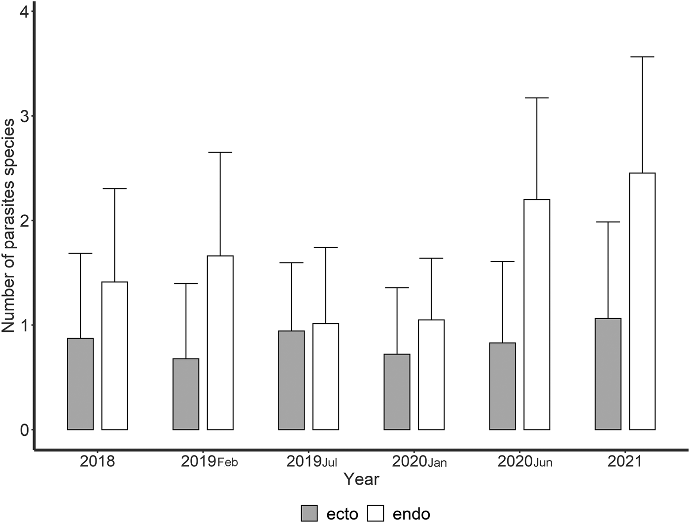
Twenty-five taxa of metazoan parasites (15 helminth species and ten Crustacea) were identified, and 9648 individual parasites recovered from 421 L. peru collected from Acapulco Bay, Mexico. Two of these species were Monogenea (adults), seven were Digenea (six adults and one metacercaria), one was Acanthocephala (adult), one was Cestoda (larvae), four were Nematoda (one adult and three larvae), seven were Copepoda, and three were Isopoda (table 1). The best represented parasite groups were the digeneans and the copepods, with 28% of total recovered species each. Based on infection site, twelve parasite species were classified as ectoparasites and thirteen as endoparasites. Endoparasite species numbers (fig. 1) varied significantly from 1.01 ± 0.72 in July 2019 to 2.45 ± 1.11 in April 2021 (ANOVA F 5,420 = 30.42, P < 0.01), and were higher than those of ectoparasites in most of the samples (fig. 1).
Box plot of species number of ectoparasites (monogenean and crustacean), and endoparasites (larvae and adults) in Lutjanus peru from Acapulco Bay.

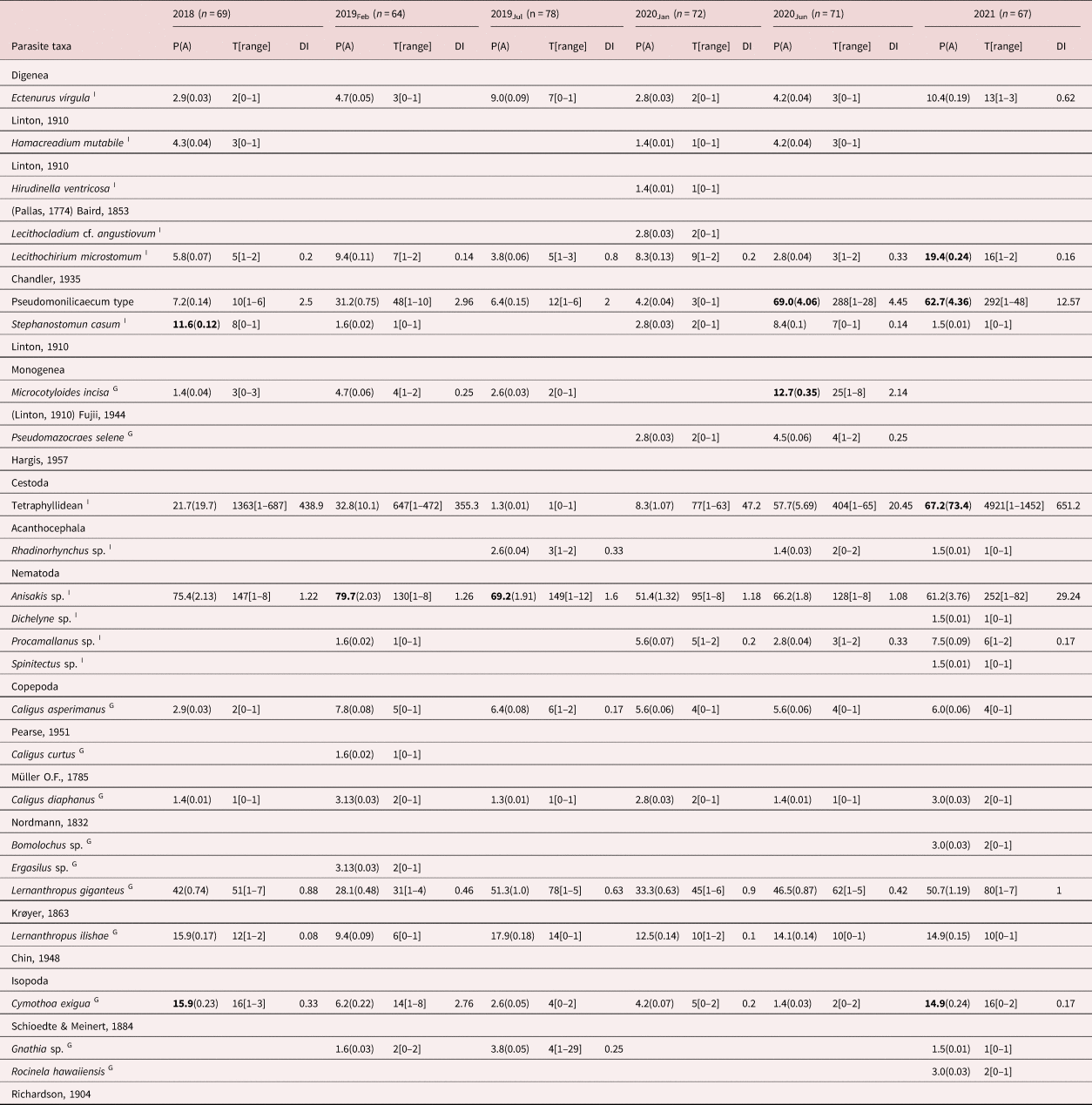
Parasite infection parameters for Lutjanus peru from Acapulco Bay. Site of infection: I = intestine, G = gills. P = prevalence, (A) = number of parasites per fish, T = total number of individual parasites collected, [range] = minimum to maximum number of parasites present, DI = variance to mean ratio. Subscripts to the right of the sampling year indicate the sampling month: Jan = January, Feb = February, Jun = June, Jul = July. Significantly different measurements of prevalence (G-test) and abundance (factorial analysis of variance) (P < 0.05), are in boldface type.

Interannual variation in infection levels
Eleven parasite species occurred in the L. peru parasite communities in all or most samplings (table 1), but only for five of these widely-distributed species prevalence varied significantly, although no clear interannual variation pattern was observed. For example, the digenean Pseudomonilicaecum type (G = 143.8, P < 0.05) and tetraphyllidean cestode (G = 111.3, P < 0.05) registered higher infection percentages during the last two samplings (January 2020 and April 2021, table 1). For the digenean Stephanostomun casum prevalence was highest during August 2018 (G = 16.3, P < 0.05), and for Lecithochirium microstomum during April 2021 (G = 11.6, P < 0.05). While the isopod Cymothoa exigua (G = 11.6, P < 0.05) exhibited its highest prevalence during the first and last sampling date (August 2018 and April 2021, table 1). Only four of these parasite species (except for C. exigua) exhibited significant interannual variation in their mean abundance (GLM: ANOVA P < 0.5). Prevalence values correlated positively with mean abundance values, indicating that the most prevalent parasite species were also the most abundant (rs = 0.958, P < 0.01, n = 73).
Relationship between the host body size and the infection parameters
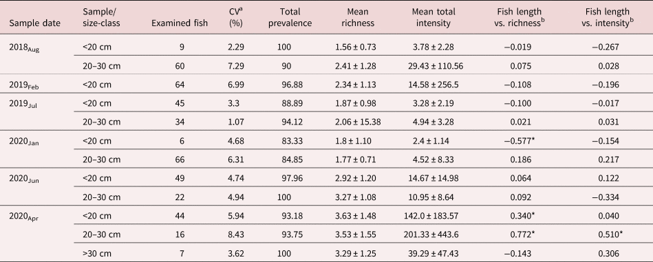
Host body size correlated negatively with the abundance values of some of the parasite taxa; for example. Ectenurus virgula (rs = −0.102, P < 0.05, n = 421), Pseudomonilicaecum type (rs = −0.198, P < 0.01, n = 421) and the tetraphyllidean cestode (rs = −0.161, P < 0.01, n = 421). Analyses of host size-classes by sampling date (table 2) also indicated that mean species richness and mean total intensity tended to decrease from the smallest to largest size-classes in some samples (table 2). No correlation was observed between the total number of examined fish in each size-class and mean species richness (rs = −0.098, P > 0.05, n = 12), or mean total intensity (rs = −0.098, P > 0.05, n = 12) indicating that the different sample sizes used in this analysis did not affect the results.
Relationships between host body size and the parasite infection parameters for Lutjans peru from Acapulco Bay. Subscripts to the right of the sampling year indicate the sampling month: Jan = January, Feb = February, Apr = April, Jun = June, Jul = July, Aug = August.

a Coefficient of variation in fish length (%).
b Spearman rank correlation coefficient.
* Significant at P < 0.05.
Spatial dispersion
The DI values indicated that at least five parasite taxa (20%) exhibited an aggregate dispersion pattern in one or more samplings (table 1). Higher mean aggregation values (DI > 5) occurred in several samplings for the digenean Pseudomonilicaecum type, tetraphyllidean cestode and the nematode Anisakis sp. (table 1). The DI values of each parasite taxa correlated positively with its prevalence (rs = 0.636, P < 0.01), total number of individuals (rs = 0.802, P < 0.01, n = 73), and mean abundance (rs = 0.795, P < 0.01, n = 73) values, but not with host body size or sample size (P > 0.05, n = 73).
Host diet composition
The alimentary spectrum of L. peru included 11 prey items of which crab larvae (27.4%), amphipods (26.7%) and snail larvae (14.4%) represented the largest proportions. Additonal prey items accounted for 31.5% of the diet, and included stomatopods, clam larvae, young octopus, penneid larvae, and small fish, among others. Diet composition varied between sampling date (t = 2.99; d.f. = 5, P < 0.05). For example, in April 2021 diet composition was more varied (H = 0.845, table 3), with crab larvae being the main prey of L. peru. Feeding habit also changed with fish body size, since larger individuals (>30 cm) consumed higher percentages of fish, while smaller ones (<20 cm) fed on higher percentages of crustaceans and other prey.
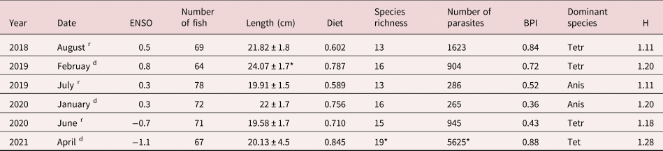
Characteristics of the parasite component communities in the Pacific red snapper Lutjanus peru from Acapulco Bay.

ENSO = multivariate El Niño index (positive values represent the warm phase, while negative values the cooling phase), Length = total length, Diet = diet variety, BPI = Berger–Parker index; H = Shannon–Wiener diversity index. Anis = Anisakis sp., Tetr = tetraphyllidean. Numbers and letters as superscripts represent codes of assignment ranges of locations and climatic seasons (d = dry, r = rainy) used in the multivariate statistical analysis.
*Significant at P < 0.05.
Component community
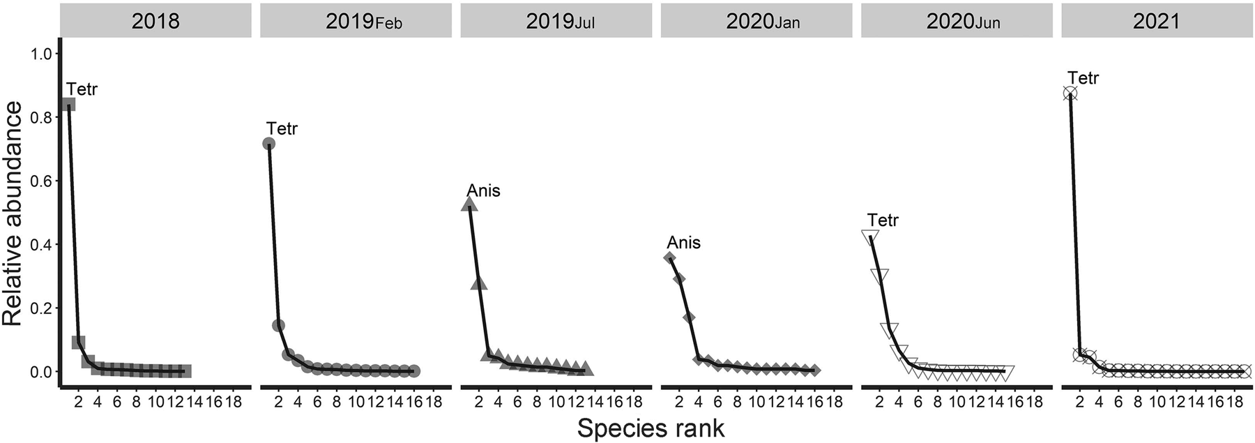
Parasite species richness by sampling date (table 3) varied from 13 (August 2018 and July 2019) to 19 (April 2021) (Kruskal–Wallis test = 87.96, d.f. = 5, P < 0.01). No correlation was observed between sample size and species richness at this level (rs = −0.530, P > 0.05, n = 5). The total number of individual parasites ranged from 265 (January 2020) to 5655 (April 2021) (Kruskal–Wallis test = 108.51, d.f. = 5, P < 0.01). The digenean Pseudomonilicaecum type, and the tetraphyllidean cestode numerically dominated the parasite communities (table 3). Shannon–Wiener diversity index values were generally high for all samplings dates (H > 1.10). Rank-abundance curves (fig. 2) showed that parasite species abundance distribution changed notably throughout the study period. Although abundance distribution in all samples was best described by a log-series model (fig. 2), the parasite communities exhibited a gradual decline in abundance of the dominant species during most of the study period, followed by an increase at the end of the period (fig. 2).
Range-abundance curves for parasite component communities in Lutjanus peru, from Acapulco Bay.

Between component communities, similarity varied widely from 8.83% (January 2020–April 2021) to 68.79% (February 2019–June 2020).
Infracommunities
Lutjanus peru body size ranged from 19.58 ± 1.7 cm (June 2020) to 24.07 ± 1.7 cm (February 2019) (table 3) and differed between sampling dates (ANOVA F 5,420 = 35.9, P < 0.05). The infracommunity parameters varied sgnificanly between sampling dates. Mean parasite species richness varied from 1.77 ± 0.74 to 2.96 ± 1.54 (GLM: ANOVA F 5,420 = 23.57, P < 0.05), mean number of individual parasites from 4.03 ± 2.8 to 89.29 ± 232.7 (GLM: ANOVA F 5,420 = 6.29, P < 0.05) and Brillouin diversity index (H’) values varied from 0.38 ± 0.35 to 0.85 ± 0.37 (GLM: ANOVA F 5,420 = 12.36, P < 0.05). All infracommunity parameters generally exhibited the same pattern, tending to decrease during the first four samples and increase in the last two (fig. 3). When considering all the samples, mean diversity (rs = −0.107, P < 0.05, n = 421) and mean number of parasite individuals (rs = −0.113, p < 0.05, n = 421) exhibited negative correlations with host body.
Mean values of the infracommunity parameters (±standard deviation) in Lutjanus peru from Acapulco Bay.

Multivariate analyses
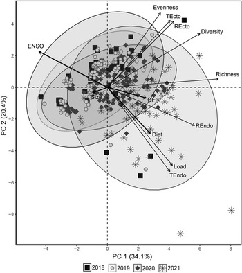
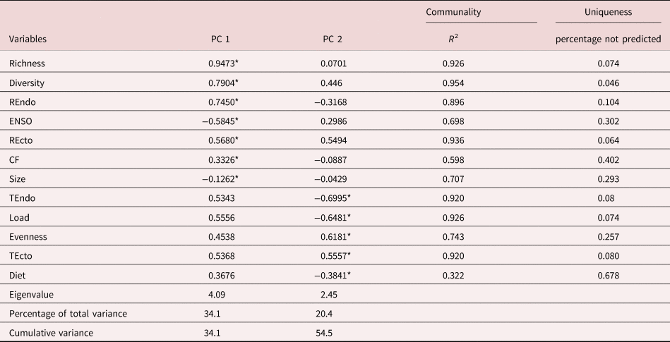
In the PCA applied to identify the possible influence of biotic and abiotic factors on parasite infracommunity structure (fig. 4), the first two component variables generated by the model explained 49% of total variance: they contributed 29.6% (eigenvalue = 4.14) and 19.4% (eigenvalue = 2.71), respectively. The first component variable associated the fish condition factor, sampling year and climatic anomalies with the diversity and species richness parameters (table 4).
Scatter plot of principal component analysis (PCA) of factors that influence the species richness and diversity of the parasite infracommunities of Lutjanus peru, from Acapulco Bay. Predictor variables: size = host body size (total length), CF = condition factor, Year = sampling year, Season = climatic season (dry/rainy), Diet = host diet variety, ENSO = multivariate El Niño index values. Infracommunity parameters: REcto = number of ectoparasite species, REndo = number of endoparasite species, TEcto = total number of ectoparasites, TEndo = total number of endoparasites, Diversity = Brillouin diversity index values, Evenness = species evenness, Richness = number of parasite species per host.

Summary of the principal component analysis (PCA) on biotic and abiotic factors that influence the diversity and species richness of the infracommunities of Lutjanus peru. The first and second principal component axes are indicated by PC 1 and PC 2, respectively. Variables that contribute to the total explained variance in each principal component are indicated by an asterisk. Eigenvalues, percentage of variance and cumulative variance are shown at the end of the table. Communality = total influence of the variable with respect to all other associated variables. Uniqueness = percentage of variability that is not predicted by the variable in the model.

Richness = Number of parasite species per host, Diversity = Brillouin diversity index values, REndo = number of endoparasite species, ENSO = Multivariate El Niño index values, REcto = number of ectoparasite species, CF = condition factor, Size = host body size (total length), TEndo = total number of endoparasites, Load = total number of parasites per infracommunity, Evenness = species evenness, TEcto = total number of ectoparasites, Diet = host diet variety.
This variable indicated that fish with better condition and a varied diet were collected during the last sampling years, when water surface temperature was slightly cooler (table 4). Both diversity and parasite species richness were higher in the parasite infracommunities of these fish. The second variable associated the host body size, climatic season and diet variety with the total and endoparasite loads (table 4).
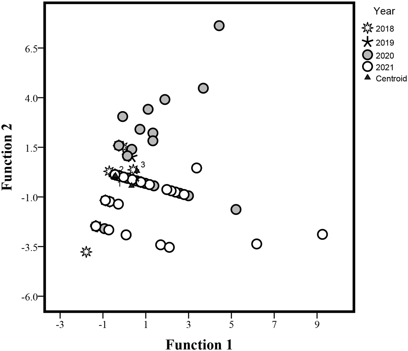
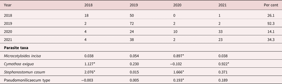
In the model constructed to identify possible interannual differences in parasite community structure, the first two discriminant variables explained 84.7% of total variance, contributing 63.7% (eigenvalue = 0.217) and 21% (eigenvalue = 0.071), respectively. A significant overall group effect was observed (Wilks’ lambda = 0.729, P < 0.001). Individual fish were mainly distributed along the first axis (fig. 5). Dimensionality tests showed that the four sampling years were significantly different in both dimensions (χ 2 = 88.42, d.f. = 12, P < 0.001). Each fish was correctly classified to one of the four sampling years with a 43.2% accuracy, which is almost double that achieved by chance alone (25%). Of the 12 selected component species (i.e. prevalence >10%), only four were accepted by the model (table 5) based on their lower Wilks’ lambda values. High abundance of the monogenean Microcotyloides incisa was characteristic of hosts collected in April 2020. The digenean S. casum and the isopod C. exigua effectively functioned to assign hosts to August 2018, while the digenean Pseudomonilicaecum type distinguished between hosts from June 2020 and April 2021.
Graphic of multivariate discriminant analyses for parasite infracommunities of Lutjanus peru, from Acapulco Bay. The symbols represent each one of the fish examined during each sampling year. Centroid = mean group.

Discriminant analysis classification showing the numbers and percentages of the Lutjanus peru classified in each sampling year (rows correspond to group memberships). The bottom of the table, shows the matrix of classification coefficient values for parasites that allowed differentiation between sampling years; asterisks indicate the importance of each parasite species in distinguishing among years.

Discussion
Parasite community species composition
All the recorded parasite species (15 helminths and ten crustaceans) are new geographical records for L. peru on the Pacific coast of Mexico (table 1). Parasite communities of L. peru were characterized for having greater species richness of digenean and copepods (seven species each); indeed, these parasite groups represented 56% of the total species recovered. In tropical regions, digeneans are the most diverse group of helminth parasites in fish from all environments (fresh, marine and brackish water) (Luque & Poulin, Reference Luque and Poulin2007; Violante-González et al., Reference Violante-González, Aguirre-Macedo and Mendoza-Franco2007; García-Prieto et al., Reference García-Prieto, Mendoza-Garfias and Perez-Ponce de Leon2014). Copepods are also a highly diverse group, that mainly parasitize marine fish (Morales-Serna et al., Reference Morales-Serna, Pinacho-Pinacho, Gomez and Perez-Ponce de León2014; Soler-Jiménez et al., Reference Soler-Jiménez, Morales-Serna and Aguirre Macedo2019).
Lutjanid fish are usually parasitized by copepods of the Caligidae, Acanthosomatidae and Dichelesthiidae families (Pilla et al., Reference Pilla, Vankara and Chikkam2012; Morales-Serna et al., Reference Morales-Serna, Pinacho-Pinacho, Gomez and Perez-Ponce de León2014), but there are few reports of these crustaceans as parasites in lutjanids from the Pacific coast of Mexico (Morales-Serna et al., Reference Morales-Serna, Pinacho-Pinacho, Gomez and Perez-Ponce de León2014). Endoparasites represented 94% of the total individual parasites recovered in this host species. Fish species with carnivorous habits, such as L. peru, tend to be associated with higher parasite species numbers and total endoparasite loads, which they acquire by consuming infected prey (Luque et al., Reference Luque, Mouillot and Poulin2004; Miranda-Delgado et al., Reference Miranda-Delgado, Violante-González, Monks, Rojas-Herrera, García-Ibáñez, Flores-Rodríguez, Romero-Ramírez and Santos-Bustos2019; Santos-Bustos et al., Reference Santos-Bustos, Violante-González, Monks, Villalba-Vásquez, Salas-Villalobos, Acosta-Hernández and Diaz-Gallegos2020).
Interannual variation in parasite infection levels
At least five parasite taxa (four endoparasites – Lecithochirium microstomum, Pseudomonilicaecum type, S. casum and a Tetraphyllidae cestode; and one ectoparasite – C. exigua) exhibited significant interannual differences in infection levels (table 1). Endoparasites are trophically-transmitted, so variations in their infection levels can be explained by interannual changes in host diet and availability of prey harbouring infective stages (Garcias et al., Reference Garcias, Mendoza and George-Nascimento2001; Luque et al., Reference Luque, Mouillot and Poulin2004; Iannacone et al., Reference Iannacone, Moron and Guizado2010; Miranda-Delgado et al., Reference Miranda-Delgado, Violante-González, Monks, Rojas-Herrera, García-Ibáñez, Flores-Rodríguez, Romero-Ramírez and Santos-Bustos2019; Santos-Bustos et al., Reference Santos-Bustos, Violante-González, Monks, Villalba-Vásquez, Salas-Villalobos, Acosta-Hernández and Diaz-Gallegos2020).
Like other snappers, L. peru is considered an opportunistic carnivorous predator with variations in its feeding behaviour linked to age, location and climatic season (Santamaría-Miranda et al., Reference Santamaría-Miranda, Elorduy-Garay, Villalejo-Fuerte and Rojas-Herrera2003; Rojas-Herrera et al., Reference Rojas-Herrera, Mascaro and Chiappa-Carrara2004; Moreno-Sánchez et al., Reference Moreno-Sánchez, Abitia-Cárdenas, Trujillo-Retana, Navia, Ramírez-Pérez and Shirasago-German2016). In other words, L. peru feeds on the prey which are more abundant during a specific season or at a specific location. The present results show that the diet of L. peru is more variable in some years and/or climatic seasons (table 3).
The crustacean isopod C. exigua is considered a common parasite of the lutjanids (Ruiz & Madrid, Reference Ruiz and Madrid1992). It was more prevalent in August 2018 and April 2021 (table 1), during different local environmental conditions (ENSO warming and cooling phases, respectively), suggesting that its occurrence and abundance may not be influenced by changes in water temperature, as has been observed in other crustacean ectoparasites (Hamre et al., Reference Hamre, Bui, Oppedal, Skern-Mauritzen and Dalvin2019).
Importance as intermediate host
The numerical dominance of the Pseudomonilicaecum type, the tetraphyllidean cestode and the nematode Anisakis sp. in the parasite communities of L. peru indicates that this fish can act as an intermediate host for these intestinal parasites during its life cycle. The didymozoid Pseudomonilicaecum type matures in scombrid fishes (Madhavi & Ram, Reference Madhavi and Ram2000; Mele et al., Reference Mele, Macias, Gomez-Vives, Garippa, Alemany and Merella2012); the nematode Anisakis sp. matures in marine mammals (Moravec, Reference Moravec1998); and the unidentified tetraphyllidean cestode uses elasmobranch fish as definitive hosts (Khalil et al., Reference Khalil, Jones and Bray1994). This suggests that younger L. peru individuals could be a prey species for these final hosts. The negative correlations between the abundance of Pseudomonilicaecum type, and tetraphyllidean cestode with the host body size, indicate that smaller L. peru were more heavily parasitized by these helminths. Helminths’ larvae are transmitted to their definitive hosts via predation, meaning that the fish functioning as intermediate hosts are usually smaller in size (Luque & Poulin, Reference Luque and Poulin2004).
Dispersion pattern
Aggregation is considered a typical dispersion pattern of many parasite speces in marine fish (Rohde, Reference Rohde2005; Iannacone et al., Reference Iannacone, Moron and Guizado2010; Amarante et al., Reference Amarante, Tassinari, Luque and Pereira2015). However, the widely variable aggregation levels of three parasite taxa (the digenean Pseudomonilicaecum type, tetraphyllidean cestode and the nematode Anisakis sp.) suggest the existence of differences in host exposure rates to parasites over time. Differing exposure rates could be due to the influence of local environmental factors (Poulin, Reference Poulin2013), or differences in host feeding behaviour between years and climatic seasons, as revealed in the diet analysis of L. peru (table 3). On the other hand, some studies suggest that DI values can be influenced by differences in sample size (Poulin, Reference Poulin1993), but there was no positive correlation between DI values and sample sizes in the present analysis.
Component communities
Species richness at the component level (13–19 species, table 3) was similar to that reported for other Lutjanus species: L. Lutjanus guttaus (19 species); Lutjanus campechanus (21 species); Lutjanus synagris (25 species); and Lutjanus griseus (20 species) (Argáez-García et al., Reference Argáez-García, Guillén-Hernández and Aguirre-Macedo2010; Montoya-Mendoza et al., Reference Montoya-Mendoza, Jiménez-Badillo, Salgado-Maldonado and Mendoza-Franco2014, Reference Montoya-Mendoza, Castañeda-Chávez, Lango-Reynoso and Rojas-Castañeda2016; Morales-Serna et al., Reference Morales-Serna, García-Vargas, Medina-Guerrero and Fajer-Ávila2017). However, the overall parasite fauna for L. peru was 25 species even though the highest species richness registered at the component level was 19 parasite species (April 2019, table 3). Rank-abundance curves of parasite species have been used to represent changes in parasite community structure over time (Norton et al., Reference Norton, Lewis and Rollinson2004; Poulin et al., Reference Poulin, Luque, Guilhaumon and Mouillot2008). The rank-abundance curves (fig. 2) constructed for each of the L. peru parasite community suggest that relative abundance of the numerically dominant species changed remarkably between sampling years. For example, the degree of dominance of the most abundant species within the community changed year on year, and there was also alternation between two dominant species (fig. 2). Similarity in species composition between parasite communities was generally low (mean = 37.8%), which can be attributed to the fact that 37% (nine species: four endoparasites and five ectoparasites) of the identified parasite species occurred on only one or two sampling dates (table 1). This suggests that species composition in the L. peru parasite communities can be unstable and may vary due to the addition of rare species. However, species diversity was high at this study level (table 3), indicating low aggregate variability (Micheli et al., Reference Micheli, Cottingham and Bascompte1999); that is, there was greater stability or repeatability in this parameter of the structure of this parasite community. According to Micheli et al. (Reference Micheli, Cottingham and Bascompte1999), the possible variability scenario of the parasite community of L. peru could be in compensation phase (i.e. high compositional variability and low aggregate variability). This result suggests that ontogenetic changes in diet, as well as interannual variations in prey consumption, could have affected the relative importance of prey types at each ontogenetic level, causing variations between years in the relative abundance of each taxon of parasite and this in the parasite species composition (Garcias et al., Reference Garcias, Mendoza and George-Nascimento2001); although other characteristics of the community structure such as species diversity, remained stable over the years. Similar results have been reported for other parasite communities of marine fish. The parasite communities of Cilus gilberti and Scartichthys viridis, had high compositional variability and low aggregate variability (i.e. richness, abundance, diversity and dominance values) (Balboa & George-Nascimento, Reference Balboa and George-Nascimento1998; Garcias et al., Reference Garcias, Mendoza and George-Nascimento2001; Díaz &George-Nascimento, Reference Díaz and George-Nascimento2002).
Infracommunities
Several biotic and abiotic factors are important determinants of species richness and diversity in parasite communities (Timi & Poulin, Reference Timi and Poulin2003; Luque et al., Reference Luque, Mouillot and Poulin2004; Gallegos-Navarro et al., Reference Gallegos-Navarro, Violante-González, Monks, García-Ibáñez, Rojas-Herrera, Pulido-Flores and Rosas-Acevedo2018; Villalba-Vásquez et al., Reference Villalba-Vásquez, Violante-González, Monks, Marino-Romero, García-Ibáñez, Rojas-Herrera, Flores-Garza and Rosas-Guerrero2018; Santos-Bustos et al., Reference Santos-Bustos, Violante-González, Monks, Villalba-Vásquez, Salas-Villalobos, Acosta-Hernández and Diaz-Gallegos2020). The PCA results (fig. 4) indicated that variations in the diet and differences in the host body size were important factors that generated interannual changes in the parasite infracomunity structure, confirming previous results.
Host diet is vital in structuring the intestinal parasite infracommunities of marine fish (Sasal et al., Reference Sasal, Morand and Guegan1997; Luque et al., Reference Luque, Mouillot and Poulin2004), while the host body size has proved to be the main predictor of total species richness of parasites (Sasal et al., Reference Sasal, Morand and Guegan1997; Luque et al., Reference Luque, Mouillot and Poulin2004). Large body size can facilitate parasite colonization since larger individuals tend to ingest greater quantities of food and are older, meaning they have had more time to accumulate parasites than smaller individuals (Timi & Poulin, Reference Timi and Poulin2003; Luque et al., Reference Luque, Mouillot and Poulin2004; Luque & Poulin, Reference Luque and Poulin2008; Villalba-Vásquez et al., Reference Villalba-Vásquez, Violante-González, Monks, Marino-Romero, García-Ibáñez, Rojas-Herrera, Flores-Garza and Rosas-Guerrero2018). In L. peru, however, body size had a more important effect in the structuring of parasite infracommunities in smaller fish than in larger ones, as indicated by the PCA results (size: r = −0.1262, table 4). This also supported by the negative correlations between host body size and the abundance of the helminths E. vírgula, Pseudomonilicaecum type and tetraphyllidean cestode; as well as between host body size and two infracommunity parameters (diversity and number of parasite individuals). These patterns suggest that the more complex infracommunity structure observed in smaller fish did not result from a difference in periods of parasite accumulation and infection exposure, as has been suggested for other host species (Luque & Chaves, Reference Luque and Chaves1999; Campos et al., Reference Campos, Fonseca, Takemoto and Moraes2009; Villalba-Vásquez et al., Reference Villalba-Vásquez, Violante-González, Monks, Marino-Romero, García-Ibáñez, Rojas-Herrera, Flores-Garza and Rosas-Guerrero2018).
Rather, the higher prevalence or abundance of some parasites in small L. peru specimens may be the result of other factors such as young fish acquiring parasites that are later eliminated when they mature (e.g. via development of an immune reaction in older organisms), and/or the intermediate hosts preyed on by young fish may differ from those preyed on by older fish (Luque & Chaves, Reference Luque and Chaves1999; Campos et al., Reference Campos, Fonseca, Takemoto and Moraes2009; Villalba-Vásquez et al., Reference Villalba-Vásquez, Violante-González, Monks, Marino-Romero, García-Ibáñez, Rojas-Herrera, Flores-Garza and Rosas-Guerrero2018; Violante-González et al., Reference Violante-González, Monks, Gallegos-Navarro, Santos-Bustos, Villalba-Vásquez, Padilla-Serrato and Pulido-Flores2020). For example, small fish (<20 cm) had a more variable diet than pre-adult and adult fish, meaning they may have been more exposed than larger fish to a greater number of infective endoparasites from a broader range of parasite taxa than the larger ones (Villalba-Vásquez et al., Reference Villalba-Vásquez, Violante-González, Monks, Marino-Romero, García-Ibáñez, Rojas-Herrera, Flores-Garza and Rosas-Guerrero2018; Violante-González et al., Reference Violante-González, Monks, Gallegos-Navarro, Santos-Bustos, Villalba-Vásquez, Padilla-Serrato and Pulido-Flores2020). Analyses of host size-classes by sampling date (table 2) also indicated that mean species richness and mean total intensity tended to decrease inversely with fish size-classes in some of the samples (e.g. January 2020, June 2020 and April 2021, table 2).
Parasites are known to be useful as biological tags in distinguishing between fish marine stocks of the same species (Timi, Reference Timi2007; Poulin & Kamiya, Reference Poulin and Kamiya2015; Violante-González et al., Reference Violante-González, Monks, Gallegos-Navarro, Santos-Bustos, Villalba-Vásquez, Padilla-Serrato and Pulido-Flores2020), but the parasite fauna method has only rarely been applied to quantify any possible variation in community structure and species composition over time (Violante-González et al., Reference Violante-González, Monks, Gallegos-Navarro, Santos-Bustos, Villalba-Vásquez, Padilla-Serrato and Pulido-Flores2020). The discriminant analysis results (table 5) indicated that the high variation in the infection levels of at least four parasite species (the monogenean M. incisa, the digeneans Pseudomonilicaecum type and S. casum; and the isopod C. exigua) may generate substantial interannual changes in the parasite community structure of L. peru in Acapulco Bay.
Conclusions
Overall, the parasite communities of L. peru were characterized by high numerical dominance of endoparasite larvae. The communities had high variability in species composition, but low aggregate variability, suggesting that other features of the community structure such as the diversity and species richness may be quite stable over time. Therefore, a clear pattern of interannual variation was not observed, indicating that each parasite species of L. peru may respond differently to environmental changes. Variations in community structure probably were due to factors such as host traits (e.g. feeding behaviour and body size) and possible interannual differences in environmental factors and availability of infected prey.
Acknowledgements
The authors thank the fishermen who caught the fish in each sampling date, as well as to the students of the Marine Ecology Faculty (UAGro) for their assistance with field, and laboratory work. Two anonymous reviewers provided useful comments that substantially improved this manuscript.
Conflicts of interest
None.
Financial support
The Consejo Nacional de Ciencia y Tecnología (CONACYT) provided a scholarship (no. 780025) to P.J.V.-D.
Ethical standards
In this study we examined fish obtained from commercial catches, so the populations of Lutjanus peru were not affected.