1. Introduction
A key public health consideration throughout the COVID-19 pandemic has been when and how to act to control the disease. In infectious disease epidemiology there is a balance to be struck between rapid introduction of control measures to limit the size of an epidemic outbreak and the costs (for example, economic, social, and mental health costs) associated with control measures. Given that the probability of a small epidemic outbreak can be close to 1 for a super-critical epidemic (basic reproduction number
 $R_0 >1$
), it is important to utilise information from the epidemic outbreak to decide whether or not intervention will be cost-effective at any given point in time.
The control of an epidemic outbreak, whether it is at a national or local level, needs to take place early in the outbreak, before the disease has taken significant hold within the population. During the early stages of an epidemic, a branching process approximation can be utilised (see [Reference Ball2], [Reference Ball and Donnelly3], and [Reference Whittle19]), with the probability of a small epidemic equated with the extinction probability of the approximating branching process. Therefore, a significant focus of this paper is on modelling the approximating branching process.
Branching process approximations of epidemic processes are built upon coupling infective individuals to individuals in a branching process, with infectious contacts and removals of infectives respectively corresponding to births and deaths in the branching process. At any point in time, given the current state of the population, we can then compute properties of the branching process (epidemic), such as the probability of extinction. However, in reality we rarely know the current state of the population and instead have a partial observation of the epidemic process; see, for example, [Reference O’Neill and Roberts15] and [Reference Trapman and Bootsma18]. Typically, we do not know when an individual becomes infected, but we can have information on when they show symptoms. Specifically, we consider susceptible–infectious–removed (SIR) epidemic models where all individuals, except an initial infective, start in the susceptible state. A susceptible individual on receiving an infectious contact becomes infected, and immediately infectious, and is able to infect other individuals until their removal (for example, through recovery, quarantining, or death). Removed individuals play no further role in the epidemic. Moreover, we assume that individuals are potentially detected on removal but nothing is known about infectious individuals prior to removal. This corresponds to observing only some of the deaths of individuals in the approximating branching process.
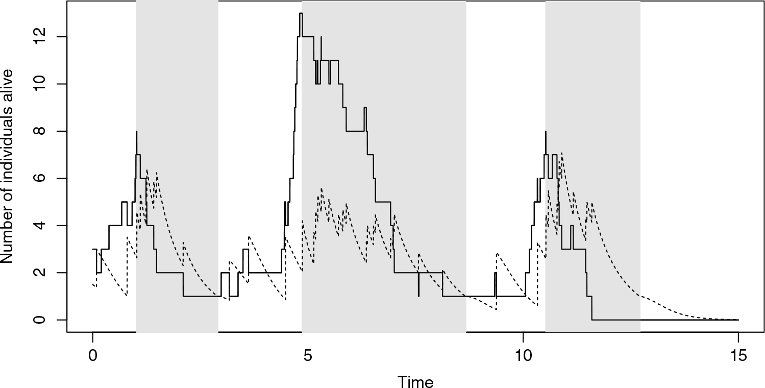
This paper’s focus is the distribution of the number of infectives in an epidemic (the number of individuals alive in a branching process) at any given point in time,
 $t \geq 0$
, based upon only the detected removals (deaths) up to and including time t, with the first detected removal (death) being observed at time
 $t=0$
. We focus primarily on the case where all removals are detected. We consider a time-inhomogeneous Markovian SIR epidemic model and its approximating branching (birth–death) process. For time-inhomogeneous epidemics, the approximating branching process has a varying environment, and all individuals alive at a given point in time have the same birth rate. The environment can depend upon the number of removals/deaths observed (cf. [Reference O’Neill14]). We show that the distribution of the number of individuals alive in the approximating branching process at time
 $t \geq 0$
can be expressed as a mixture of
 $(k_t+1)$
negative binomial random variables, where
 $k_t$
denotes the total number of observed deaths/removals up to and including time t. Given that we allow for time-inhomogeneity in the model, we are able to derive the distribution of the number of infectives in the presence of control measures or seasonal effects which change the infection and/or the removal rates. In particular, given only removal data, we can easily obtain the probability that the epidemic is over, and hence provide a guide for when to lift control measures.
The papers [Reference Lambert and Trapman9] and [Reference Trapman and Bootsma18] consider the distribution of the number of individuals alive in a branching process at the first detection, where each individual is detected an exponentially distributed time after their birth (infection) assuming that they are still alive (infectious) at their detection time. Individuals are assumed to have independent and identically distributed lifetime distributions and, whilst alive, to reproduce at the points of a homogeneous Poisson point process with rate
 $\alpha$
, say. These papers show that the population size at the first detection follows a geometric distribution with support
 $\mathbb{N}$
, and [Reference Lambert and Trapman9] studies further properties of the population at the first detection, such as the ages of individuals and the residual lifetimes. A key tool in [Reference Lambert and Trapman9] is to obtain the (shifted geometric) distribution of the population t units after the birth of the initial individual, conditional upon there being no detections up to time t. We take the same approach in this paper to obtain, in Section 4, Lemma 4.1, a geometric distribution with support
 $\mathbb{N}$
for the size of the population t units after the birth of the initial individual, conditional upon there being no deaths up to time t. The Markovian models considered in this paper allow for explicit expressions for the parameters of the geometric distribution, in contrast to [Reference Lambert and Trapman9], where the key quantities are expressed in terms of Laplace transforms. Moreover, we allow for time-inhomogeneity in the model in both the birth and death rates. In [Reference Lefèvre, Picard and Utev11], a birth–death process with detections is considered, and this corresponds to the model of [Reference Lambert and Trapman9] with an exponential lifetime distribution. In [Reference Lefèvre, Picard and Utev11], the distribution of the number of individuals alive at the kth detection is considered, but times between detections are not considered. Finally, in [Reference Lefèvre and Picard10] the general stochastic epidemic model (i.e. the Markovian SIR epidemic model with exponentially distributed infectious periods) is considered, with detections possibly occurring at the removal of individuals; the authors investigate the distribution of the number of infectives at the kth detection. Both [Reference Lefèvre and Picard10] and [Reference Lefèvre, Picard and Utev11] allow for the parameters of the models to change at the detection times. Since we consider the full time dynamics of the branching (epidemic) process, we can allow for more general temporal behaviour of the parameters, but an important special case is where the parameters are piecewise constant between detection times.
The paper is structured as follows. In Section 2, we introduce the time-inhomogeneous Markovian SIR epidemic model and its branching (birth–death) process approximation. In Section 3, we present the main result, Theorem 3.1, which shows that the distribution of the number of individuals alive in the birth–death process, given only death times, can be expressed as a mixture of negative binomial distributions. This is extended in Theorem 3.2 to the case where only a subset of the death times are detected. The probability that the birth–death process will go extinct and the likelihood of observing a given set of death times, given in Corollary 3.1, follow immediately from Theorem 3.1. In Theorem 3.3 we derive the exact distribution of the number of infectives in the SIR epidemic given only removal times, which is useful for assessing the accuracy of the birth–death process approximations. In Sections 4–6 we provide the proofs of Theorems 3.1–3.3 respectively. In Section 7 we present numerical results using simulations to illustrate the estimation of the number of individuals over time, the implementation of control measures, and comparisons between the number of infectives in the epidemic and the number of individuals alive in the approximating birth–death process. In particular, a time-inhomogeneous birth–death process is shown to give a good approximation of the epidemic process over its full trajectory. Finally, in Section 8 we present concluding remarks regarding how the findings of this paper can be utilised from statistical inference and public health perspectives.
2. Epidemic and branching process models
In this section, we introduce formally the time-inhomogeneous Markovian SIR epidemic model and its approximating branching (birth–death) process.
The time-inhomogeneous Markovian SIR epidemic model is defined as follows. There is assumed to be a closed population of size N with the epidemic initiated by a single infective in an otherwise susceptible population. Whilst infectious, individuals make infectious contacts at the points of a time-inhomogeneous Poisson point process with rate
 $\beta_t$
at time t. The individual contacted by an infectious contact is chosen uniformly at random from the whole population, independently of any other infectious contacts. If a susceptible individual is contacted by an infectious contact, the individual becomes infected and is immediately able to transmit the disease to other individuals. Infectious contacts with non-susceptible individuals have no effect on the recipient. Infective individuals recover from the disease and are removed from the epidemic process, playing no further role in the epidemic, at rate
 $\gamma_t$
at time t. Let S(t), I(t), and
 $R(t)\;(= N - S(t) - I(t))$
denote the total numbers of susceptibles, infectives, and removed individuals, respectively, in the population at time t. Then it suffices to keep track of
 $\{ (S(t), I(t) )\}$
, and the model satisfies, for
 $h \geq 0$
,
 \begin{align} & \mathbb{P} \left( (S(t+h),I(t+h)) = (x,y) \left| (S(t),I(t)) = (s,i) \right. \right) \nonumber \\[5pt] & \qquad = \left\{ \begin{array}{l@{\quad}l@{\quad}l} \dfrac{s i}{N} \beta_t h + o(h), & (x,y) =(s-1,i+1) & \textrm{(infection)}, \\[9pt] i \gamma_t h + o(h), & (x,y) =(s,i-1) & \textrm{(removal)}, \\[5pt] 1 - i \left\{ \beta_t \frac{s}{N} + \gamma_t \right\} h + o(h), & (x,y) =(s,i) & \textrm{(no event)}, \end{array} \right. \end{align}
with all other events occurring with probability o(h). We place no restriction on the form of
 $\beta_t$
and
 $\gamma_t$
, and these could be continuously varying and/or contain discontinuities. The former can be used to model seasonal variability, whilst the latter allows for the implementation and removal of control measures.
In the early stages of the epidemic, whilst the total number of individuals ever infected is small, the epidemic process can be coupled to a branching process. Specifically, each infective in the epidemic has a corresponding individual in the coupled branching process whose lifetime is identical to the infectious period of the infective, so the individual in the branching process dies when the infective is removed from the population. The individual in the branching process gives birth to new individuals whenever the corresponding infective makes infectious contacts in the epidemic process. Thus the two processes can be coupled (see, for example, [Reference Ball and Donnelly3]) until the first time that there is an infectious contact with a previously infected individual. For large N this does not occur until
 $O(\sqrt{N})$
of the population have been infected; see [Reference Ball and Donnelly3]. Specifically, the time-inhomogeneous Markovian SIR stochastic epidemic model can be approximated by a time-inhomogeneous linear birth–death process [Reference Kendall8]. Let B(t) denote the total number of individuals alive in the time-inhomogeneous linear birth–death process at time t. Then for
 $h \geq 0$
, B(t) satisfies
 \begin{align} \mathbb{P} (B (t + h) = j | B(t) = i) = \left\{ \begin{array}{l@{\quad}l@{\quad}l} i \beta_t h + o(h), & j = i+1& \mbox{(birth)}, \\[5pt] i \gamma_t h + o(h), & j = i-1 & \mbox{(death)}, \\[5pt] 1 - i \{ \beta_t + \gamma_t \} h+ o(h), & j = i & \mbox{(no event)}, \\[5pt] \end{array} \right. \end{align}
with all other events occurring with probability o(h).
Suppose that at time t we can estimate the proportion,
 $s_t$
, of the population who are susceptible in the epidemic process. We can then replace
 $\beta_t$
by
 $\beta_t s_t$
in (2.2) to obtain a birth–death approximation of the epidemic which is valid after the epidemic has taken off. In Section 7 we outline a simple estimate of
 $s_t$
using only the inter-removal times, up to and including time t, to create a time-inhomogeneous birth–death process approximation to the epidemic process. In Figure 4 we show the excellent agreement between the estimates obtained from these two processes of the mean number of infectives at time t, given only the inter-removal times up to and including time t.
3. Main results
3.1. Overview
In this section, we present the main results along with the necessary notation. Throughout, we set time so that the first death (removal) of the birth–death (epidemic) process occurs at time 0. The time-varying parameters in (2.1) and (2.2) can be adjusted accordingly.
In Section 3.2 we present Theorem 3.1, which states that the distribution of the number of individuals alive in a time-inhomogeneous linear birth–death process given only times of deaths follows a mixture of negative binomial distributions. We present an outline of the arguments used to prove Theorem 3.1, with the details of the proof provided in Section 4. We note that Theorem 3.1 allows computation of the probability that the birth–death process will go extinct. In Corollary 3.1 we derive the likelihood of observing the given death times, which can be used in statistical inference for inferring the parameters of the birth–death process given data.
In Section 3.3, we consider the special case of the time-homogeneous linear birth–death process. Lemma 3.1 specialises Theorem 3.1 to the time-homogeneous birth–death process and Lemma 3.2 gives the distribution of the number of individuals alive in the birth–death process immediately after the kth death, conditioning only upon there having been k deaths. The proof of Lemma 3.2 is presented immediately after the lemma and is informative about why, in general, the distribution of the number of individuals alive follows a mixture of negative binomial distributions.
In Section 3.4, we consider the important extension of assuming that not all deaths are detected. In Theorem 3.2, we show that the number of individuals alive given only the times of detected deaths follows a mixture of negative binomial distributions. The overall structure of the proof is similar to that of Theorem 3.1, but there are key differences, as Lemma 4.1, which is a major component in the proof of Theorem 3.1, does not carry over to partial detection of deaths. Therefore we need to resort to an alternative argument based on probability generating functions, whose details are provided in Section 5. In Section 3.5, Theorem 3.3, we derive the number of infectives in the general stochastic epidemic model at time t given only the times of removals. This enables us, in Section 7, to compare the approximate distribution given by the birth–death process for the number of infectives (individuals alive) with the exact distribution given by Theorem 3.3. For succinctness of presentation in Sections 3.4 and 3.5, we assume that the birth (infection) and death (removal) parameters are piecewise constant between observed deaths (removals), although more general piecewise-constant parameter scenarios could easily be considered.
3.2. Time-inhomogeneous linear birth–death process
For
 $k=1,2,\ldots$
, let
 $X_k$
denote the number of individuals alive immediately after the kth death, and for
 $t \geq 0$
, let Y(t) denote the number of individuals alive at time t, with
 $Y(0) \equiv X_1$
. For
 $k=2,3,\ldots$
, let
 $T_k$
denote the inter-arrival time from the
 $(k-1)$
th to the kth death, with the convention that
 $T_k = \infty$
if fewer than k deaths occur, and let
 $S_k = \sum_{j=2}^k T_j$
denote the time of the kth death, with
 $S_1 =0$
. Let
 $\textbf{T}_{2:k} = (T_2, T_3, \ldots, T_k)$
. For
 $k=2,3,\ldots$
, let
 $t_k$
denote the observed inter-arrival time from the
 $(k-1)$
th to the kth death and
 $s_k =\sum_{j=2}^k t_j$
, with
 $s_1 =0$
. For
 $k =2,3, \ldots$
, let
 $\textbf{t}_{2:k} = (t_2, t_3, \ldots, t_k)$
; we consider the distribution of
 $X_k | \textbf{T}_{2:k} = \textbf{t}_{2:k}$
. For
 $t \geq 0$
, let
 $k_t$
denote the number of deaths, and let
 $s_{k_t}$
denote the time of the last death, up to and including time t. Then for
 $t \geq 0$
, we consider the distribution of
 $Y(t) | \textbf{T}_{2:k_t} = \textbf{t}_{2:k_t}$
. Note that
 $Y (s_k) \equiv X_k$
, which is used repeatedly.
Before stating Theorem 3.1 we introduce some notation for probability distributions. Throughout this paper,
 $G \sim \textrm{Geom}(p)$
denotes a geometric random variable with parameter p and probability mass function
 \begin{equation} \mathbb{P} (G = x) = (1-p)^x p \hspace{0.5cm} (x=0,1,\ldots). \end{equation}
Also, for
 $r=0,1,\ldots$
,
 $V = \sum_{i=1}^r G_i \sim \textrm{NegBin}(r,p)$
denotes a negative binomial random variable, where
 $G_1, G_2, \ldots, G_r$
are independent and identically distributed according to
 $\textrm{Geom}(p)$
, and for
 $r=0$
,
 $\mathbb{P}(V =0) =1$
.
Theorem 3.1 starts with the assumption that there exists
 $0 < \pi_0 <1$
such that
 $X_1 \equiv Y(0) \sim \textrm{Geom} (\pi_0)$
. In the important special case where the birth and death rates are constant prior to the first death—that is, for
 $t \leq 0$
,
 $\beta_t = \alpha_1$
, and
 $\gamma_t = \mu_1$
—it is trivial (cf. the start of the proof of Lemma 3.2) to show that the number of individuals alive immediately after the first death is
 $\textrm{Geom } (\pi_0)$
with
 $\pi_0 = \mu_1/(\alpha_1 + \mu_1)$
. (See also [Reference Lambert and Trapman9] and [Reference Trapman and Bootsma18].) We discuss how the arguments can be modified to other scenarios in Section 4, after the proof of Theorem 3.1.
Theorem 3.1.
Suppose that
 $X_1 \equiv Y(0) \sim \textrm{Geom} (\pi_0)$
for some
 $0 < \pi_0 <1$
.
For
 $t \geq 0$
, let
 $\pi_t$
solve the ordinary differential equation (ODE)
 \begin{eqnarray} \pi_t^\prime = \gamma_t - (\beta_t + \gamma_t) \pi_t,\end{eqnarray}
with initial condition
 $0 < \pi_0 <1$
.
For
 $k =2,3, \ldots$
, the distribution
 $X_k$
of the number of individuals alive immediately following the kth death satisfies
 \begin{eqnarray} \{X_k |\textbf{T}_{2:k} = \textbf{t}_{2:k}\} \sim \textrm{NegBin} (R_k,\pi_{s_k}), \end{eqnarray}
where
 $R_k$
is a random variable with support on
 $\{2,3,\ldots, k\}$
, and
 $\mathbb{P} (R_k =j) = B_{k,j}$
with
 $\textbf{B}_k =(B_{k,2}, B_{k,3}, \ldots, B_{k,k})$
given by (3.11) below.
For
 $t \geq 0$
, the distribution Y(t) of the number of individuals alive at time t satisfies
 $Y(t) \equiv X_{k_t}$
if
 $t = s_{k_t}$
, and if
 $t>s_{k_t}$
,
 \begin{eqnarray} \{Y (t)|\textbf{T}_{2:k_t} = \textbf{t}_{2:k_t} \} \sim \textrm{NegBin} (Z(t),\pi_t), \end{eqnarray}
where Z(t) is a random variable with support on
 $\{0,1,\ldots, k_t\}$
, and
 $\mathbb{P} (Z(t)=j) = D_{t,j}$
with
 $\textbf{D}_t = (D_{t,0}, D_{t,1}, \ldots, D_{t,k_t})$
given by (3.12) and (3.13) below. If
 $k_t =1$
, then
 $T_2 > t$
replaces
 $\textbf{T}_{2:k_t} = \textbf{t}_{2:k_t}$
in (3.4).
We begin by defining the notation required to obtain the distributions of
 $R_k$
and Z(t) introduced in Theorem 3.1. The process
 $\{Z(t)\;:\; t \ge 0\}$
is clarified in the proof of Corollary 4.1. Briefly, it is an integer-valued stochastic process that decreases in steps of size 1 between deaths until either it reaches 0, in which case the number of individuals alive is 0 and no further deaths occur, or a death occurs, in which case Z(t) increases by 1. The process
 $\{Z(t)\;:\; t \ge 0\}$
is Markovian given also the death times prior to t. We also further explore
 $\pi_t$
before presenting an outline of the main steps in the proof of Theorem 3.1, with the details provided in Section 4.
For
 $t \in \mathbb{R}$
, let
 $p_t = \beta_t / \{\beta_t + \gamma_t\}$
(resp.
 $q_t = \gamma_t/\{\beta_t + \gamma_t\}$
) denote the probability that an event occurring at time t is a birth (resp. death). Then for
 $t \geq 0$
, we can rewrite the ODE (3.2) for
 $\pi_t$
as
 \begin{eqnarray} \pi_t^\prime = (\beta_t + \gamma_t) [q_t - \pi_t],\end{eqnarray}
with initial condition
 $0 < \pi_0 <1$
. This highlights that
 $\pi_t$
is increasing (decreasing) if
 $q_t > \pi_t$
(
 $q_t < \pi_t$
), with
 $\pi_0$
defined by the birth and death rates prior to the first death.
For
 $t, \tau \geq 0$
, let
 \begin{eqnarray} \phi (t;\; \tau) = \exp\!\bigg( - \int_t^{t+\tau} \{ \beta_s + \gamma_s \} \, ds \bigg),\end{eqnarray}
the probability that an individual alive at time t does not give birth or die in the interval
 $(t, t+\tau]$
, and let
 \begin{eqnarray} \psi(t;\; \tau) = \int_t^{t+\tau} \beta_u \exp \!\bigg( - \int_{u}^{t+\tau} \{\beta_s + \gamma_s \} \, ds \bigg)\, du, \end{eqnarray}
the probability that an individual alive at time t has at least one offspring and their first offspring (looking back from time
 $t+ \tau$
) survives to time
 $t+ \tau$
. We can then rewrite (3.2) in integral form as
 \begin{align} \pi_{t+\tau} &= \pi_t \exp\!\bigg( - \int_t^{t+\tau} \{ \beta_s + \gamma_s \} \, ds \bigg) + \int_t^{t+\tau} \gamma_u \exp\!\bigg( - \int_u^{t+\tau} \{ \beta_s + \gamma_s \} \, ds \bigg) \, du \nonumber \\[5pt] &= \pi_t \phi (t;\; \tau) + \{1 - \phi (t;\; \tau) - \psi (t;\;\tau) \}.\end{align}
We can now define the matrices needed for the probability mass functions of
 $R_k$
and Z(t), which define the distributions of
 $X_k$
and Y(t) in Theorem 3.1. For
 $k=2,3,\ldots$
and for
 $t,\tau \geq 0$
, let
 $\textbf{M}_k (t;\;\tau)$
be the
 $(k-1) \times k$
matrix with (i, j)th element
 \begin{align} [\textbf{M}_k (t;\;\tau)]_{i,j} &= \left\{ \begin{array}{l@{\quad}l} (i+1) \binom{i}{j-1} \bigg\{\dfrac{(1-\pi_t) \pi_t}{(1-\pi_{t+\tau}) \pi_{t+\tau}} \phi (t;\;\tau)\bigg\}^{j-1} \bigg\{\dfrac{\pi_t }{1- \pi_{t+\tau}} \psi(t;\; \tau) \bigg\}^{i+1-j} & \!\!\mbox{for } j \leq i+1, \\[10pt] 0 & \!\!\mbox{otherwise}, \end{array} \right. \nonumber \\ & \end{align}
and let
 $\textbf{J}_k (t;\;\tau)$
be the
 $(k-1) \times (k+1)$
matrix with (i, j)th element
 \begin{eqnarray} [\textbf{J}_k (t;\;\tau)]_{i,j} = \left\{ \begin{array}{l@{\quad}l} \binom{i+1}{j-1} \bigg\{\dfrac{(1-\pi_t) \pi_t}{(1-\pi_{t+\tau}) \pi_{t+\tau}} \phi (t;\;\tau) \bigg\}^{j-1} \bigg\{ \dfrac{\pi_t}{1-\pi_{t+\tau}} \psi(t;\; \tau) \bigg\}^{i+2-j} & \mbox{for } j \leq i+2, \\[10pt] 0 & \mbox{otherwise}. \end{array} \right. \nonumber \\[5pt] \end{eqnarray}
Let
 $\textbf{B}_2 = (1)$
, and for
 $k=3,4,\ldots$
let
 $\textbf{B}_k=(B_{k,2}, B_{k,3}, \ldots, B_{k,k})$
be given by
 \begin{eqnarray} \textbf{B}_{k} = \Bigg\{ \Bigg( \prod_{j=2}^{k-1} \textbf{M}_j (s_j;\; t_{j+1}) \Bigg) \cdot \textbf{1}_{k-1}^\top\Bigg\}^{-1} \prod_{j=2}^{k-1} \textbf{M}_j (s_j;\; t_{j+1}),\end{eqnarray}
with
 $\textbf{1}_{k-1}$
denoting a row vector of 1s of length
 $k-1$
. Let
 $\textbf{D}_t =(D_{t,0}, D_{t,1}, \ldots, D_{t,k_t})$
be given by, for
 $0 \leq t < s_2$
,
 \begin{eqnarray} \textbf{D}_t = \bigg( \frac{\pi_t \psi(0;\;t)}{\pi_t \psi(0;\;t)+(1-\pi_0) \phi (0;\;t)}, \frac{(1-\pi_0) \phi (0;\;t)}{\pi_t \psi(0;\;t)+(1-\pi_0) \phi (0;\;t)} \bigg), \end{eqnarray}
and for
 $t \geq s_2$
,
 \begin{align} \textbf{D}_t &= \Bigg\{ \Bigg( \prod_{j=2}^{k_t -1} \textbf{M}_j (s_j;\; t_{j+1}) \Bigg) \textbf{J}_{k_t} (s_{k_t};\;t-s_{k_t}) \cdot \textbf{1}_{k_t+1}^\top\Bigg\}^{-1} \nonumber \\[5pt] &\quad \times \Bigg( \prod_{j=2}^{k_t -1} \textbf{M}_j (s_j;\; t_{j+1}) \Bigg) \textbf{J}_{k_t} (s_{k_t};\;t-s_{k_t}), \end{align}
with the convention
 $\prod_{j=2}^{1} \textbf{M}_j (s_j;\;t_{j+1}) =\textbf{I}_1$
(the
 $1 \times 1$
identity matrix).
To prove Theorem 3.1, we start by showing in Lemma 4.1 that the number of living individuals at time
 $t + \tau$
originating from a single individual at time t, conditional on no deaths in the interval
 $(t, t+\tau]$
, is
 $1 + \textrm{Geom} (1- \psi(t;\; \tau))$
. This is proved using a probabilistic construction of the process. We can use this to consider how the birth–death process evolves between the first and second death when we have
 $\textrm{Geom } (\pi_0)$
rather than one initial individual. In Lemma 4.3, we show that for any given time t between the first and second deaths, the distribution of the number of individuals alive follows a mixture of a geometric distribution,
 $G_1 (\pi_{t}) \sim \textrm{Geom} (\pi_t) $
, and a point mass at 0. This leads, through size-biased sampling in Lemma 4.4, to the number of individuals alive immediately after the second death (time
 $s_2 =t_2$
) being distributed as a negative binomial distribution,
 $\sum_{i=1}^{2} G_i (\pi_{s_2}) =\textrm{NegBin} (2, \pi_{s_2})$
.
Finally, the dynamics of the process between the first and second death, along with the Markovian nature of the process, allow us to relatively straightforwardly write down the full dynamics. In particular, given that
 $\{X_k | \textbf{T}_{2:k} = \textbf{t}_{2:k}\} = \sum_{i=1}^{R_k} G_i (\pi_{s_k}) $
, we can consider the evolution of
 $R_k$
independent processes each starting from
 $\textrm{Geom} (\pi_{s_k}) $
individuals. At time
 $s_{k+1}$
, the
 $(k+1)$
th death will occur, and the death will belong to one of the
 $R_k$
processes starting with
 $\textrm{Geom} (\pi_{s_k}) $
individuals. The process with the death will have
 $\textrm{NegBin} (2, \pi_{s_{k+1}})$
individuals alive at time
 $s_{k+1}$
to contribute to
 $X_{k+1}$
. The remaining
 $R_k-1$
processes will have experienced no deaths in the interval
 $(s_k, s_{k+1}]$
, and the number of individuals alive in each of these processes is distributed according to a mixture of
 $\textrm{Geom} (\pi_{s_{k+1}})$
and a point mass at 0. This leads to the binomial terms in (3.9) and (3.10) for the number of processes which have
 $\textrm{Geom} (\pi_{s_{k+1}})$
individuals alive; see Corollary 4.1. It is then straightforward, using Lemma 4.5, to iteratively compute the distribution of
 $\{X_k | \textbf{T}_{2:k} = \textbf{t}_{2:k}\}$
and complete the proof of Theorem 3.1.
We briefly discuss some interesting results which follow straightforwardly from Theorem 3.1.
Given that Theorem 3.1 provides the probability mass function of Z(t), it is straightforward to compute moments of Y(t), the number of individuals alive at time t. However, the forms of (3.4) and (3.13) do not permit any simplifications for rapid calculations of the moments of Y(t).
From [Reference Kendall8, Equation (18)] we have that at time t, the probability of non-extinction of the time-inhomogeneous birth–death process from a single individual is
 \begin{eqnarray} \rho_t = \bigg\{ 1 + \int_t^\infty \gamma_s \exp\!\bigg( \int_t^s [ \gamma_u - \beta_u ] \, du \bigg)ds \bigg\}^{-1}. \end{eqnarray}
Therefore, given
 $\textbf{t}_{2:k_t}$
, at time t we have that the probability that the birth–death process will go extinct is
 \begin{eqnarray} \mathbb{E} \Big[ \left. (1 - \rho_t)^{Y(t)} \right| \textbf{T}_{2:k_t} = \textbf{t}_{2:k_t} \Big] = \mathbb{E} \Bigg[ \!\left. \bigg( \frac{\pi_t}{1-(1-\pi_t) (1-\rho_t)} \bigg)^{Z(t)} \right| \textbf{T}_{2:k_t} = \textbf{t}_{2:k_t} \!\Bigg]. \end{eqnarray}
It is straightforward to compute the right-hand side of (3.15) using the probability mass function of Z(t), which is given by (3.13). Note that if, for all
 $u \geq t$
,
 $\beta_u = \alpha$
and
 $\gamma_u = \mu$
, then
 $\rho_t = 1 - \min \{1,\mu/\alpha \}$
, and (3.15) gives the probability of extinction if the current birth and death rate were to persist.
We can compute the likelihood of observing inter-death times
 $\textbf{t}_{2:k}$
using Corollary 3.1.
Corollary 3.1.
For
 $k=2,3,\ldots$
and
 $s_k < \infty$
, we have that the probability density function of
 $\textbf{T}_{2:k}$
is given by
 \begin{eqnarray} f_{\textbf{T}_{2:k}} (\textbf{t}_{2:k}) = \prod_{j=2}^{k} \frac{\pi_{s_{j-1}} ( 1 - \pi_{s_{j-1}}) \gamma_{s_j} \phi (s_{j-1};\; t_j)}{\pi_{s_j}^2} \times \Bigg\{ \Bigg[\prod_{j=2}^{k-1} M_j (s_j;\;t_{j+1}) \Bigg] \cdot \textbf{1}_{k-1}^\top \Bigg\}, \nonumber \\[5pt] \end{eqnarray}
with, for
 $k=2$
, the vacuous latter term set equal to 1.
Corollary 3.1 is the key result in using the findings of this paper for statistical inference and inferring the parameters of the birth–death process given
 $\textbf{t}_{2:k}$
. The generality of the time-inhomogeneous birth–death process allows for different features such as the periodicity or control measures to be incorporated. We will explore likelihood inference for the birth–death process given only death times in future work.
3.3. Time-homogeneous linear birth–death process
An important special case of Theorem 3.1 is the time-homogeneous model, where, for all
 $t \in \mathbb{R}$
,
 $\beta_t = \alpha$
and
 $\gamma_t = \mu$
. In this case, for all
 $t \geq 0$
,
 \begin{align*} \pi_t =q_t= \frac{\mu}{\alpha + \mu} = \hat{\pi}, \quad \mbox{ say}, \end{align*}
and for all
 $\tau \geq 0$
,
 $\phi (t;\; \tau) = \hat{\phi} (\tau) = \exp\!\left( - [ \alpha + \mu] \tau \right)$
and
 $\psi(t;\; \tau) = \hat{\psi} (\tau) = \hat{\pi} \big\{ 1 - \hat{\phi} (\tau) \big\}$
. For
 $k=2,3,\ldots$
, let
 $\hat{\textbf{M}}_k (\tau)$
be the
 $(k-1) \times k$
matrix with (i, j)th element
 \begin{eqnarray} \Big[\hat{\textbf{M}}_k (\tau)\Big]_{i,j} = \left\{ \begin{array}{l@{\quad}l} (i+1) \binom{i}{j-1} \Big\{ \hat{\phi (\tau)}\Big\}^{j-1} \Big\{\hat{\pi} (1- \hat{\phi} (\tau) )\Big\}^{i+1-j} & \mbox{for } j \leq i+1, \\[5pt] 0 & \mbox{otherwise}, \end{array} \right.\end{eqnarray}
and let
 $\hat{\textbf{J}}_k (t;\;\tau)$
be the
 $(k-1) \times (k+1)$
matrix with (i, j)th element
 \begin{eqnarray} \Big[ \hat{\textbf{J}}_k (t;\;\tau) \Big]_{i,j} = \left\{ \begin{array}{l@{\quad}l} \binom{i+1}{j-1} \Big\{ \hat{\phi (\tau)}\Big\}^{j-1} \Big\{\hat{\pi} (1- \hat{\phi} (\tau) )\Big\}^{i+2-j} & \mbox{for } j \leq i+2, \\[5pt] 0 & \mbox{otherwise}. \end{array} \right.\end{eqnarray}
Lemma 3.1.
For the time-homogeneous birth–death process with birth rate
 $\beta_t = \alpha$
and death rate
 $\gamma_t = \mu$
, the number of individuals alive immediately following the first death at time
 $t=0$
satisfies
 \begin{align*} X_1 \equiv Y(0) \sim \textrm{Geom} (\hat{\pi}). \end{align*}
For
 $k =2,3, \ldots$
,
 $X_k$
satisfies (3.3) with
 $\pi_{s_k} = \hat{\pi}$
and
 $\textbf{B}_{k}$
given by (3.11), with
 $\hat{\textbf{M}}_k (\tau)$
given in (3.17) replacing
 $\textbf{M}_k (t;\; \tau) $
.
Similarly, for
 $t \geq 0$
, Y(t) satisfies (3.4) with
 $\pi_t = \hat{\pi}$
and
 $\textbf{D}_t$
given by (3.12) and (3.13), with
 $\hat{\textbf{M}}_k (\tau)$
and
 $\hat{\textbf{J}}_k (\tau)$
given in (3.17) and (3.18) replacing
 $\textbf{M}_k (t;\; \tau) $
and
 $\textbf{J}_k (t;\; \tau) $
, respectively.
From Lemma 3.1, we observe that
 $X_k | S_k = \sum_{j=2}^k T_j < \infty$
(conditioning on at least k deaths occurring in the birth–death process) is a mixture of negative binomial random variables
 $\{ Q_j \sim \textrm{NegBin} (j, \hat{\pi});\;\, j=2,3,\ldots,k \}$
. We can look to integrate over
 $\textbf{T}_{2:k}$
to obtain the distribution of
 $X_k | S_k < \infty$
, which can be equivalently expressed as
 $X_k |X_{k-1} >0$
. However, a direct argument, which we present below, yields Lemma 3.2 and gives a straightforward illustration of how the number of individuals alive immediately after a death follows a mixture of negative binomial distributions.
Lemma 3.2.
For
 $k=2,3,\ldots$
, let
 $\hat{R}_k$
be a discrete random variable with support
 $\{2,3,\ldots, k\}$
and probability mass function
 \begin{align*} \mathbb{P} \big( \hat{R}_k = j | X_{k-1} >0 \big) = \frac{c_{k-1,k-j} \hat{\pi}^{k-j}}{\sum_{l=2}^k c_{k-1,k-l} \hat{\pi}^{k-l}}, \hspace{0.5cm} \end{align*}
where
 $\{c_{m,j} \}$
are the entries of Catalan’s triangle (see, for example, [Reference Shapiro17]), a triangular array satisfying the following: for
 $j=0,1,\ldots$
and
 $m=1,2,\ldots$
,
 $c_{m,0} =1$
,
 $c_{m,j} = 0$
 $(j \geq m)$
, and
 \begin{eqnarray} c_{m,j} = \sum_{i=0}^j c_{m-1,i} = c_{m-1,j} + c_{m,j-1} = \frac{m-j}{m+j} \binom{m+j}{m}.\end{eqnarray}
Then for
 $k=2,3, \ldots$
,
 \begin{align*} \{X_k |X_{k-1} >0\} \sim \textrm{NegBin} (\hat{R}_k, \hat{\pi}). \end{align*}
Proof. Given that the outcome (birth/death) of each event is independent, the number of births which take place between each pair of deaths are independent and are distributed according to
 $\hat{G} \sim \textrm{Geom} (\hat{\pi})$
. Therefore, for
 $k=1,2,\ldots$
,
 \begin{eqnarray} X_k \stackrel{D}{=} X_{k-1} + \hat{G} -1,\end{eqnarray}
subject to
 $X_{k-1} >0$
. Given
 $X_0 =1$
(the birth of the initial individual), it immediately follows from (3.20) that
 $X_1 \sim \hat{G}$
.
To study
 $X_k$
 $(k>1)$
, we consider a Markov chain for the evolution of the birth–death process until the kth individual is born (which guarantees at least k deaths occur) or the process goes extinct. Let (a, d) denote the state in the Markov chain corresponding to a births and d deaths having occurred. Then for
 $k =2, 3, \ldots$
, the possible states are
 \begin{align*} \{ (a,d);\; a= 1,2, \ldots, k-1, d=0,1,\ldots, a \} \cup \{ (k,d);\; d=0, 1, \ldots, k-2 \}, \end{align*}
with a total of
 $L_k = (k+4)(k-1)/2$
possible states. The Markov chain starts in state (1,0), the birth of the initial individual, and has absorbing states
 $\mathcal{E} = \{ (x,x);\; x=1,2, \ldots, k-1\}$
(the birth–death process dies out before the kth birth) and
 $\mathcal{I} = \{ (k,d);\; d=0, 1, \ldots, k-2 \}$
(there are at least k births in the birth–death process). For
 $(a,d) \not\in \mathcal{E} \cup \mathcal{I}$
, we have that the probability of transiting from state (a, d) to state
 $(a+1,d)$
(birth) is
 $1-\hat{\pi}$
and the probability of transiting from state (a, d) to state
 $(a,d+1)$
(death) is
 $\hat{\pi}$
. Note that the process reaches an absorbing state in at most
 $2k-3$
transitions, and if the birth–death process reaches
 $a=k$
, it does so through a birth, so that there are at least two individuals alive (
 $a-d \geq 2$
).
Let
 $V_k$
denote the final (absorbing) state of the Markov chain. For
 $d=0,1,\ldots, k-2$
,
 \begin{eqnarray} \mathbb{P} (V_k = (k,d) ) = c_{k-1,d} (1-\hat{\pi})^{k-1} \hat{\pi}^d,\end{eqnarray}
where
 $\{c_{k-1,d} \}$
are the Catalan numbers given in (3.19). The derivation of (3.21) is as follows. Any path from (1,0) to (k, d) must include
 $k-1$
births and d deaths, so has probability
 $(1-\hat{\pi})^{k-1} \hat{\pi}^d$
of occurring. The admissible paths are those for which, at any point on the path, the number of births (including the initial ancestor) is always greater than the number of deaths. Therefore, the number of admissible paths is equivalent to the number of ways of counting the votes in the ballot theorem with candidates A and B having k and d votes, respectively, such that after the first vote, candidate A always has more votes than candidate B, with there being
 $c_{k-1,d}$
such paths. Hence, for
 $j=2,3,\ldots, k$
,
 \begin{align} \mathbb{P} (V_k = (k,k-j) | V_k \in \mathcal{I}) &= \frac{c_{k-1,k-j} (1-\hat{\pi})^{k-1} \hat{\pi}^{k-j}}{\sum_{l=2}^k c_{k-1,k-l} (1-\hat{\pi})^{k-1} \hat{\pi}^{k-l}} \nonumber \\[5pt] &= \frac{c_{k-1,k-j} \hat{\pi}^{k-j}}{\sum_{l=2}^k c_{k-1,k-l} \hat{\pi}^{k-l}}. \end{align}
Conditioned upon the birth–death process reaching state
 $(k,k-j)$
 $(j=2,3,\ldots, k)$
, the number of additional births until the kth death is the sum of j independent and identically distributed
 $\hat{G}$
random variables. Hence, the number of individuals alive immediately following the kth death is distributed according to
 \begin{eqnarray} \sum_{i=1}^j \hat{G}_i \sim \textrm{NegBin} (j,\hat{\pi}), \end{eqnarray}
3.4. Partial observations of deaths
We turn our attention to the case where not every death is detected. Suppose
 $\delta_t$
denotes the probability that a death at time t is detected and that the detection or otherwise of a death is independent of all other events. The epidemic model considered in [Reference Lefèvre and Picard10] can be constructed in this manner. We are in a situation similar to that studied in [Reference Lambert and Trapman9] and [Reference Lefèvre, Picard and Utev11], although in those papers (i) the death and detection processes are independent and (ii) individuals do not die upon detection.
We modify the notation slightly to take account of partial detection of the death process. For
 $k=2,3, \ldots$
, let
 $\tilde{T}_k$
denote the length of time between the
 $(k-1)$
th and kth detected deaths, with the convention that
 $\tilde{T}_1$
denotes the time from the birth of the initial individual to the first detected death (with
 $\tilde{T}_1 = \infty$
if no death is ever detected). Given that
 $\tilde{T}_1 < \infty$
, i.e. that a death is detected, we set time 0 to be the time at which the first death is detected. Let
 $\tilde{X}_k$
denote the number of individuals alive immediately after the kth detected death. In Theorem 3.2 we show that
 $\tilde{X}_k$
is a mixture of negative binomial random variables with mixture weights depending on
 $\tilde{T}_{2:k} = \tilde{t}_{2:k}$
, similarly to Theorem 3.1. Note that we set
 $\tilde{s}_k = \sum_{j=2}^k \tilde{t}_j$
.
As stated in Section 3.1, we assume that the birth and death rates are piecewise constant between detected deaths. That is, setting
 $\tilde{s}_0 = - \infty$
, we assume for
 $\tilde{s}_{k-1} < t \leq \tilde{s}_k$
that
 $(\beta_t, \gamma_t, \delta_t) = (\tilde{\alpha}_k, \tilde{\mu}_k, \tilde{d}_k)$
. Let
 $\tilde{q}_k = \tilde{\mu}_k/(\tilde{\alpha}_k + \tilde{\mu}_k)$
and
 $\tilde{p}_k = 1- \tilde{q}_k$
. Note that for
 $\tilde{s}_{k-1} < t \leq \tilde{s}_k$
,
 $q_t = \tilde{q}_k$
and
 $p_t = \tilde{p}_k$
. Let
 \begin{align} \begin{array}{ll@{\quad}ll}u_k &= \sqrt{1 - 4 \tilde{p}_k \tilde{q}_k (1-\tilde{d}_k)}, & \lambda_k &=\dfrac{1 + u_k - 2 \tilde{p}_k}{1 + u_k}, \\[10pt] \nu_k &= \dfrac{1-u_k}{2\tilde{p}_k}, & \zeta_k &= \dfrac{1 + u_k}{2\tilde{p}_k} = \dfrac{1}{1- \lambda_k}, \\[10pt] \tilde{\phi}_k (\tau) &= \exp\!(- [\tilde{\alpha}_k + \tilde{\mu}_k] u_k \tau), &\tilde{\psi}_k (\tau) &= \dfrac{(1-\lambda_k) (1- \tilde{\phi}_k (\tau)}{1- \nu_k (1-\lambda_k) \tilde{\phi}_k (\tau)}.\end{array} \end{align}
Note that if
 $\tilde{d}_k =1$
, i.e. all deaths are detected, then the above simplify to
 $u_k =1$
,
 $\lambda_k= \tilde{q}_k$
,
 $\nu_k = 0$
,
 $\zeta_k = 1/\tilde{p}_k$
,
 $\tilde{\phi}_k (\tau) = \exp\!(- [\tilde{\alpha}_k + \tilde{\mu}_k] \tau)$
, and
 $\tilde{\psi}_k (\tau) = \tilde{p}_k [1- \exp\!(- [\tilde{\alpha}_k + \tilde{\mu}_k] \tau) ]$
. Thus
 $\lambda_k$
,
 $\tilde{\phi}_k (\tau)$
, and
 $\tilde{\psi}_k (\tau) $
take the roles of
 $q_t$
,
 $\phi (t;\; \tau)$
, and
 $\psi(t;\;\tau)$
in Section 3.2.
Let
 $\tilde{\pi}_1 = \lambda_1$
, and for
 $k=2,3,\ldots$
let
 \begin{eqnarray} \tilde{\pi}_k = \frac{\lambda_k [1 - \nu_k (1-\tilde{\pi}_{k-1})] - (1-\nu_k) [ \lambda_k - \tilde{\pi}_{k-1}] \tilde{\phi}_k (\tilde{t}_k)}{1 - \nu_k (1-\tilde{\pi}_{k-1}) + \nu_k [ \lambda_k - \tilde{\pi}_{k-1}] \tilde{\phi}_k (\tilde{t}_k)}.\end{eqnarray}
Thus
 $\tilde{\pi}_k = \pi_{\tilde{s}_k}$
, the success probability of the geometric at the kth detected death, and we can modify (3.25) to obtain
 $\pi_t$
 $(t \geq 0)$
; see (3.29).
Theorem 3.2.
For the piecewise time-homogeneous linear birth–death process with parameters
 $(\beta_t, \gamma_t, \delta_t) = (\tilde{\alpha}_k, \tilde{\mu}_k, \tilde{d}_k)$
 $(\tilde{s}_{k-1} < t \leq \tilde{s}_k)$
, we have the following:
-
1.
 $\tilde{X}_1 | \tilde{T}_1 < \infty \sim \textrm{Geom} (\tilde{\pi}_1)$
.
-
2. Let
$\tilde{\textbf{B}}_2 = (1)$
, and for
$k=3,4,\ldots$
, let
$\tilde{\textbf{B}}_{k}=(\tilde{B}_{k,2}, \tilde{B}_{k,3}, \ldots, \tilde{B}_{k,k})$
be given by
(3.26)where, for
\begin{eqnarray} \tilde{\textbf{B}}_{k} = \Bigg\{ \Bigg( \prod_{j=2}^{k-1} \tilde{\textbf{M}}_j ( \tilde{t}_{j+1}) \Bigg) \cdot \textbf{1}_{k-2}^\top\Bigg\}^{-1} \prod_{j=2}^{k-1} \tilde{\textbf{M}}_j ( \tilde{t}_{j+1}),\end{eqnarray}
$\tau \geq 0$
,
$\tilde{\textbf{M}}_k (\tau)$
is the
$(k-1) \times k$
matrix with (i,j)th element
where
\begin{eqnarray*} \Big[\tilde{\textbf{M}}_k (\tau) \Big]_{i,j} = \Bigg\{ \begin{array}{l@{\quad}l} (i+1) \binom{i}{j-1} \tilde{h}_{k+1} (\tau)^{j-1} \big[1-\tilde{h}_{k+1} (\tau)\big]^{i+1-j} \tilde{r}_{k+1}(\tau)^i & \textit{for } j \leq i+1, \\[5pt] 0 & \textit{otherwise}, \end{array} \nonumber\end{eqnarray*}
(3.27)and
\begin{eqnarray} \tilde{h}_{k+1} (\tau) = \frac{1 - \tilde{\pi}_{k+1} - \tilde{\psi}_{k+1} (\tau)}{\big(1- \tilde{\pi}_{k+1}\big)\big(1- \tilde{\psi}_{k+1} (\tau)\big)}\end{eqnarray}
Then for
\begin{eqnarray*}\tilde{r}_{k+1} (\tau) = \frac{\tilde{\pi}_k \big[\lambda_{k+1} + (1-\lambda_{k+1}) (1-\nu_{k+1}) \tilde{\phi}_{k+1} (\tau)\big]}{\lambda_{k+1} \big[ 1- \nu_{k+1} \big(1-\tilde{\pi}_k\big)\big] - (1-\nu_{k+1}) \big[ \lambda_{k+1} - \tilde{\pi}_k\big] \tilde{\phi}_{k+1} (\tau)}.\end{eqnarray*}
$k=2,3,\ldots$
,
$\tilde{X}_k$
, the number of individuals alive immediately following the kth detected death, satisfies
(3.28)where
\begin{eqnarray} \big\{\tilde{X}_k |\tilde{\textbf{T}}_{2:k} = \tilde{\textbf{t}}_{2:k}\big\} \sim \textrm{NegBin} \big(\tilde{R}_k,\tilde{\pi}_k\big), \end{eqnarray}
$\tilde{R}_k$
has support
$\{2,3,\ldots, k\}$
and
$\mathbb{P} (\tilde{R}_k =j) =\tilde{B}_{k,j}$
$(j=2,3,\ldots,k)$
.
-
3. For
$k=2,3,\ldots$
, let
$\tilde{\textbf{J}}_k (\tau)$
be the
$(k-1) \times (k+1)$
matrix with (i,j)th entry
For
\begin{eqnarray*} \Big[ \tilde{\textbf{J}}_k (\tau) \Big]_{i,j} = \Bigg\{ \begin{array}{l@{\quad}l} \binom{i+1}{j-1} \tilde{h}_{k+1} (\tau)^{j-1} \big[1-\tilde{h}_{k+1} (\tau)\big]^{i+2-j} \tilde{r}_{k+1}(\tau)^{i+1} & \textit{for } j \leq i+2, \\[5pt] 0 & \textit{otherwise}. \end{array} \end{eqnarray*}
$t \geq 0$
, let
$\tilde{k}_t$
and
$\tilde{s}_{\tilde{k}_t}$
denote the number of detected deaths and the time of the last detected death, respectively, up to and including time t. Let
$\tilde{\textbf{D}}_t =(\tilde{D}_{t,0}, \tilde{D}_{t,1}, \ldots, \tilde{D}_{t,k_t})$
satisfy, for
$t < \tilde{s}_2$
,where
\begin{align*} \tilde{\textbf{D}}_t = \Bigg( \frac{\tilde{\pi}_t \tilde{\psi}_2 (t)}{(1-\tilde{\pi}_t) (1-\tilde{\psi}_2 (t))},\frac{1-\tilde{\pi}_t- \tilde{\psi}_2 (t)}{(1-\tilde{\pi}_t) (1-\tilde{\psi}_2 (t))} \Bigg), \end{align*}
(3.29)and for
\begin{eqnarray} \tilde{\pi}_t = \frac{\lambda_{\tilde{k}_t} \big[1 - \nu_{\tilde{k}_t} \big(1-\tilde{\pi}_{{\tilde{k}_t}-1}\big)\big] - \big(1-\nu_{\tilde{k}_t}\big) \big[ \lambda_{\tilde{k}_t} - \tilde{\pi}_{{\tilde{k}_t}-1}\big] \tilde{\phi}_{\tilde{k}_t} \big(t-\tilde{s}_{\tilde{k}_t}\big)}{1 - \nu_{\tilde{k}_t} \big(1-\tilde{\pi}_{{\tilde{k}_t}-1}\big) + \nu_{\tilde{k}_t} \big[ \lambda_{\tilde{k}_t} - \tilde{\pi}_{{\tilde{k}_t}-1}\big] \tilde{\phi}_{\tilde{k}_t} \big(t-\tilde{s}_{\tilde{k}_t}\big)},\end{eqnarray}
$t \geq \tilde{s}_2$
,Then Y(t) satisfies
\begin{eqnarray*} \tilde{\textbf{D}}_t = \Bigg\{ \Bigg( \prod_{j=2}^{k_t -1} \tilde{\textbf{M}}_j (t_{j+1}) \Bigg) \tilde{\textbf{J}}_{k_t} \big(t-\tilde{s}_{\tilde{k}_t}\big) \cdot \textbf{1}_{k-1}^\top\Bigg\}^{-1} \Bigg( \prod_{j=2}^{k_t -1} \tilde{\textbf{M}}_j (t_{j+1}) \Bigg) \tilde{\textbf{J}}_{k_t} \big(t-\tilde{s}_{\tilde{k}_t}\big).\nonumber \end{eqnarray*}
$Y(t) \equiv \tilde{X}_{\tilde{k}_t}$
, if
$t = \tilde{s}_{\tilde{k}_t}$
, and
where
\begin{eqnarray*} \Big\{Y (t)| \tilde{\textbf{T}}_{2:\tilde{k}_t} = \tilde{\textbf{t}}_{2:\tilde{k}_t} \Big\} \sim \textrm{NegBin} \big(\tilde{Z} (t),\pi_t\big), \nonumber \end{eqnarray*}
$\tilde{Z} (t)$
has support
$\{0,1,\ldots,k_t\}$
and
$\mathbb{P} (\tilde{Z}(t) =j) = \tilde{D}_{t,j}$
$(j=0,1,\ldots, \tilde{k}_t)$
.


3.5. General stochastic epidemic
Finally, we turn our attention to the time-inhomogeneous general stochastic epidemic, defined by (2.1) in Section 2, with one initial infective in an otherwise susceptible population of size N. Let
 $\{(S(t),I(t))\}$
denote the process of the numbers of susceptibles and infectives at time t; as with the birth–death process, we employ the convention that the first removal takes place at time 0. In a natural change of terminology for moving from the birth–death process to the epidemic process, let
 $T_k$
denote the inter-arrival time between the
 $(k-1)$
th and kth removals, and let
 $S_k$
denote the time of the kth removal, with the convention that
 $S_1=0$
.
The Markovian nature of the general stochastic epidemic model allows us to model the evolution of
 $\{(S(t),I(t))\}$
using continuous-time Markov chains; see, for example, [Reference Gani and Purdue5] and [Reference Lefèvre and Simon12]. To facilitate analysis of the model, we assume that the infection and removal parameters are piecewise constant, and for succinctness of presentation we assume, as with the birth–death process with partial detection of deaths, that the parameters are piecewise constant between removals. That is, we assume that for
 $s_{k-1} < t \leq s_k$
, between the
 $(k-1)$
th and kth removal,
 $\beta_t = \alpha_k$
and
 $\gamma_t = \mu_k$
in (2.1).
For
 $k=1,2,\ldots, N$
and
 $s_k\leq t < s_{k+1}$
, we derive the distribution of
 $ \{I(t)|\textbf{T}_{2:k} = \textbf{t}_{2:k} \}$
in Theorem 3.3 as a product of matrices which determine the transition in the number of infectives between removal events and the transition at a removal event. We continue by defining the required matrices before stating Theorem 3.3.
For
 $k=0,1,\dots,N$
, let
 \begin{align*}\Omega_k=\{(N-k-i,i)\;:\;i=1,2,\dots,N-k\}\end{align*}
be the set of states of
 $\{(S(t), I(t))\}$
in which the epidemic is still going (i.e. there is at least one infective) and precisely k removals have occurred. Give the states in
 $\Omega_k$
the labels
 $k_1, k_2,\dots,k_{N-k}$
, where the state
 $(N-k-i,i)$
has label
 $k_i$
 $(i=1,2,\dots, N-k)$
. For
 $k=0,1,\dots,N$
, let
 $\textbf{Q}_{k,k}=[q_{k_i,k_j}]$
be the
 $(N-k)\times (N-k)$
transition-rate matrix for transitions of
 $\{(S(t), I(t))\}$
within
 $\Omega_k$
. Then, using (2.1), with
 $\beta_t = \alpha_{k+1}$
and
 $\gamma_t = \mu_{k+1}$
,
 \begin{equation}q_{k_i,k_j}= \left\{\begin{array}{l@{\quad}l} -\bigg(\dfrac{\alpha_{k+1}}{N}(N-k-i)i+ \mu_{k+1} i\bigg) & \text{ if } j=i,\\[13pt] \dfrac{\alpha_{k+1}}{N}(N-k-i)i & \text{ if } j=i+1,\\[10pt] 0 & \text{ otherwise}. \end{array} \right. \end{equation}
For
 $k=0,1,\dots,N-1$
, let
 $\textbf{Q}_{k,k+1}=[q_{k_i,(k+1)_j}]$
be the
 $(N-k) \times (N-k-1)$
transition-rate matrix for transitions of
 $\{(S(t), I(t))\}$
from
 $\Omega_k$
to
 $\Omega_{k+1}$
(a removal), so that, using (2.1),
 \begin{equation*}q_{k_i,(k+1)_j}= \Bigg\{\begin{array}{l@{\quad}l} i \mu_{k+1} & \text{ if } i \in \{2,3,\dots, N-k\} \text{ and } j=i-1,\\[5pt] 0 & \text{ otherwise}. \end{array}\end{equation*}
The above partitioning of the state space differs from that of both [Reference Gani and Purdue5] and [Reference Lefèvre and Simon12], where the state space is partitioned on the basis of the number of susceptibles remaining and the focus is on the final size (number of removals) of the epidemic.
In a similar vein, for
 $k=0,1,\dots,N$
, let
 \begin{align*}\tilde{\Omega}_k=\{(N-k-j,j)\;:\;j=0,1,\dots,N-k\}\end{align*}
be the set of all states of
 $\{(S(t), I(t))\}$
in which precisely k removals have occurred. Thus
 $\tilde{\Omega}_k=\Omega_k \cup \{(N-k,0)\}$
. Let
 $\tilde{\textbf{Q}}_{k,k}$
be the
 $(N-k+1)\times (N-k+1)$
transition-rate matrix for transitions of
 $\{(S(t), I(t))\}$
within
 $\tilde{\Omega}_k$
. The elements of
 $\tilde{\textbf{Q}}_{k,k}$
are given by (3.30), except that the indices now run from 0 to
 $N-k$
. Note that the first row of
 $\tilde{\textbf{Q}}_{k,k}$
comprises all zeros as the process has been absorbed. Finally, for
 $k=0,1,\dots,N$
, let
 $\tilde{\textbf{Q}}_{k,k+1}$
be the
 $(N-k) \times (N-k)$
transition-rate matrix for transitions of
 $\{(S(t), I(t))\}$
from
 $\Omega_k$
to
 $\tilde{\Omega}_{k+1}$
. Note that
 $\tilde{\textbf{Q}}_{k,k+1}$
is the diagonal matrix with successive diagonal elements
 $\mu_{k+1},2 \mu_{k+1},\dots, (N-k) \mu_{k+1}$
.
Theorem 3.3.
Consider an epidemic satisfying (2.1) with one initial infective in an otherwise susceptible population of size N, and let
 $s_1 = 0$
, so the first removal occurs at time 0.
For
 $k=2,3,\ldots, N$
,
 $i=0,1,\ldots,N-k$
, and
 $\tau \geq 0$
, let
 \begin{align*} v_{k,i} (\tau| \textbf{t}_{2:k}) = \mathbb{P} ( I (s_k + \tau) = i | \textbf{T}_{2:k} = \textbf{t}_{2:k}, T_{k+1} >\tau), \end{align*}
with
 $v_{1,i} (\tau) = \mathbb{P} ( I ( \tau) = i | T_{2} >\tau)$
, and let
 \begin{align*} \textbf{v}_k (\tau| \textbf{t}_{2:k})= ( v_{k,0} (\tau| \textbf{t}_{2:k}), v_{k,1} (\tau| \textbf{t}_{2:k}), \ldots, v_{k,N-k} (\tau| \textbf{t}_{2:k}) ). \end{align*}
Then
 \begin{equation}\textbf{v}_{k}(\tau|\textbf{t}_{2:k})=\frac{1}{c_k(\tau)}{\textbf{u}}_1\textbf{Q}_{0,0}^{-1}\Bigg(\prod_{i=1}^{k-1}\textbf{Q}_{i-1,i}\exp\!(\textbf{Q}_{i,i}t_{i+1})\Bigg)\tilde{\textbf{Q}}_{k-1,k}\exp\!\big(\tilde{\textbf{Q}}_{k,k}\tau\big),\end{equation}
where
 ${\textbf{u}}_1$
is the row vector of length N whose first element is 1 and all other elements are 0,
 \begin{equation}c_k(\tau)=\textbf{u}_1\textbf{Q}_{0,0}^{-1}\Bigg(\prod_{i=1}^{k-1}\textbf{Q}_{i-1,i}\exp\!(\textbf{Q}_{i,i}t_{i+1})\Bigg)\tilde{\textbf{Q}}_{k-1,k}\exp\!(\tilde{\textbf{Q}}_{k,k}\tau)\cdot \textbf{1}_{N+1-k}^\top,\end{equation}
and the product in (3.31) is equal to
 $\textbf{I}_{N-1}$
if
 $k=1$
.
Also setting
 $\tau=0$
in (3.31) yields the conditional distribution of the number infected immediately after the kth removal, given only the removal times. Note that
 $\exp\!(\tilde{\textbf{Q}}_{k,k} 0) = \textbf{I}_{N-k+1}$
.
The key difference from the approach for the birth–death process is the effect of the finite size of the population, which means that infectives do not behave independently, but that for moderate N, matrix multiplication directly yields the distribution of I(t) given only removal times. To obtain the distribution of I(t) we require matrix exponentials and matrix multiplication with the initial matrices of size
 $N \times N$
. By comparison, the computation of the distribution of Z(t) involves successive vector–matrix multiplication with the largest matrices of size
 $(k_t -1) \times (k_t +1)$
. Therefore, it is much faster to compute the distribution of Z(t), and subsequently the distribution of Y(t), than the distribution of I(t).
4. Time-inhomogeneous Markov model
In this section, we study the time-inhomogeneous linear birth–death process, with the main aim of proving Theorem 3.1. We begin by assuming that at time
 $t=0$
(the first death),
 $X_1 \sim \textrm{Geom} (\pi_0)$
for some
 $0 < \pi_0 <1$
. For example, if the birth and death rates are constants,
 $\alpha_1$
and
 $\mu_1$
respectively, prior to the first death, then we can follow Section 3.3 and obtain
 $\pi_0 = \alpha_1/(\alpha_1 + \mu_1)$
. We address the distribution of
 $X_1$
(Y(0)) more fully at the end of this section, after the proof of Theorem 3.1.
The first step to proving Theorem 3.1 is to show how the birth–death process progresses between death events. In Lemma 4.1 we show that if we start with one initial individual at time t, then given that no deaths have been observed by time
 $t+\tau$
, the number of offspring originating from the initial individual follows a geometric distribution. Before stating and proving Lemma 4.1 we introduce some notation.
For a non-negative, integer random variable W,
 $t \geq 0$
, and
 $\tau >0$
, let
 $E_{t,\tau}^W$
and
 $D_{t,\tau}^W$
respectively denote the events that there are no deaths in the interval
 $[t, t+\tau)$
and that the first death in the birth–death process after time t is at time
 $t+ \tau$
, given that there are W individuals in the population at time t. For
 $w \in \mathbb{N}$
, if
 $\mathbb{P} (W=w) =1$
, we employ the convention
 $E_{t,\tau}^w$
.
Lemma 4.1.
For
 $t \geq 0$
and
 $\tau >0$
, let
 $Y^{(t)} (\tau)$
denote the number of individuals alive at time
 $t + \tau$
, given that one individual is alive at time t. Then for
 $n \in \mathbb{N}$
,
 \begin{eqnarray} \mathbb{P} \Big(Y^{(t)} (\tau)=n, E_{t,\tau}^{1} \Big)= \psi (t;\; \tau)^{n-1} \phi (t;\; \tau), \end{eqnarray}
where
 $\phi (t;\; \tau) = \exp\!\Big( - \int_t^{t+\tau} (\beta_s + \gamma_s) \; ds \Big)$
and
 $\psi (t;\; \tau) = \int_t^{t + \tau} \beta_u \exp\!\Big(\!-\!\int_u^{t+\tau} (\beta_s + \gamma_s)ds\Big)du$
(see (3.6) and (3.7)). Therefore, we have that
 \begin{eqnarray} \mathbb{P}\big(E_{t,\tau}^{1}\big) = \frac{\phi (t;\; \tau)}{1 -\psi (t;\; \tau)} , \end{eqnarray}
and
 \begin{eqnarray} Y^{(t)} (\tau) | E_{t,\tau}^{1} \sim 1+ \textrm{Geom} (1- \psi (t;\; \tau)). \end{eqnarray}
Proof. The proof is similar to the exploration process in [Reference Lambert and Trapman9, Section 2].
First, we note that the probability that the initial individual survives to time
 $t + \tau$
is
 $\exp\!\Big( - \int_t^{t+\tau} \gamma_s \, ds \Big)$
. We then start at time
 $t+\tau$
and explore the lifeline of the initial individual back from time
 $t + \tau$
until we either discover an offspring or reach time t. The probability that we reach time t, i.e. that the initial individual has no offspring, is
 $\exp\!\Big(- \int_t^{t + \tau} \beta_s \, ds \Big)$
, with
 $\exp\!\Big( - \int_t^{t+\tau} \gamma_s \, ds \Big) \times \exp\!\Big(- \int_t^{t + \tau} \beta_s \, ds \Big) = \phi (t;\; \tau)$
.
The (defective) probability density function for the time of the first offspring, looking back from time
 $t+\tau$
, is
 $\beta_u \exp\!\left( - \int_{t+u}^{t+\tau} \beta_s \, ds \right) $
. Therefore the probability that the initial individual has at least one offspring and their first offspring (looking back from time
 $t+\tau$
) survives to time
 $t+\tau$
is given by
 $\psi (t;\; \tau)$
. If the initial individual has at least one offspring and their first offspring survives to time
 $t +\tau$
, then we repeat the above process of exploring lifelines back from time
 $t+\tau$
until we either discover an offspring or reach time t. This will start with the offspring’s lifeline, and if they have no offspring, we will continue with the unexplored lifeline of the initial individual. The total length of the lifeline to explore is again of length
 $\tau$
, and therefore, as above, the probability of no additional offspring is
 $\exp\!\left(- \int_t^{t+\tau} \beta_s \, ds \right)$
, while the probability of at least one offspring and that the first offspring discovered survives until time
 $t+\tau$
is
 $ \psi (t;\; \tau)$
. We can repeat this process by at each stage considering the combined unexplored lifelines of length
 $\tau$
and whether or not an offspring is discovered, and if an offspring is discovered whether or not it survives to time
 $t+\tau$
. This yields (4.1).
By summing over n in (4.1), we have (4.2), and (4.3) follows immediately.
Before we consider the birth–death process evolving from a random number of individuals at time t, and specifically a geometrically distributed number of individuals in Lemma 4.3, we give the following elementary lemma concerning the sums of geometric random variables, which will prove useful throughout the remainder of the paper.
Lemma 4.2.
Let
 $X, Y_1, Y_2,\dots$
be independent, with
 $X \sim \textrm{Geom}(q_1)$
and
 $Y_i \sim 1+\textrm{Geom}(q_2)$
 $(i=1,2,\dots)$
. Let
 \begin{align*}Z=\sum_{i=1}^X Y_i,\end{align*}
where
 $Z=0$
if
 $X=0$
. Then
 \begin{eqnarray*} Z \stackrel{D}{=} \left\{ \begin{array}{l@{\quad}l} \tilde{X} & \textit{with probability } \dfrac{1-q_1}{1-q_1q_2}, \\[14pt] 0 & \textit{with probability } \dfrac{q_1 (1-q_2)}{1-q_1q_2} , \end{array} \right. \nonumber \end{eqnarray*}
where
 $\tilde{X} \sim \textrm{Geom}(q_1q_2)$
.
Proof. This is elementary using probability generating functions. An alternative, more constructive, proof is available by noting that if
 $X' \sim 1+\textrm{Geom}(q_1)$
and
 $Y_i \sim 1+\textrm{Geom}(q_2)$
 $(i=1,2,\dots)$
are independent then
 $\sum_{i=1}^{X'} Y_i \sim 1+\textrm{Geom}(q_1q_2)$
.
For
 $t \geq 0$
, let
 \begin{eqnarray} G_t \sim \textrm{Geom} (\pi_t),\end{eqnarray}
where
 $\pi_t$
is given by (3.2) with initial condition
 $\pi_0$
satisfying
 $0 < \pi_0 <1$
.
Lemma 4.3.
For
 $t \geq 0$
, suppose that the number of individuals alive in a birth–death process at time t is distributed according to
 $G_t$
. For
 $\tau >0$
, let
 $W_t (\tau)$
denote the number of individuals alive at time
 $t+\tau$
. Then
 \begin{eqnarray} W_t (\tau) |E_{t;\;\tau}^{G_t} \stackrel{D}{=} \left\{ \begin{array}{l@{\quad}l} G_{t+\tau} & \textit{with probability } h (t;\; \tau) = \dfrac{(1 -\pi_t) \phi (t;\; \tau)}{(1- \pi_{t+\tau}) [1 - \psi (t;\;\tau)]}, \\[15pt] 0 & \textit{with probability } 1 - h (t;\; \tau) = \dfrac{\pi_{t+\tau} \psi(t;\; \tau)}{(1- \pi_{t+\tau}) [1 - \psi (t;\;\tau)]}. \end{array} \right. \end{eqnarray}
Proof. Firstly, using Lemma 4.1, it is easily shown that
 \begin{eqnarray*} \Big\{G_t| E_{t;\;\tau}^{G_t} \Big\} \stackrel{D}{=} \tilde{X} \sim \textrm{Geom} \bigg( 1 - \frac{ (1-\pi_t)\phi (t;\; \tau)}{1 -\psi (t;\; \tau)} \bigg). \nonumber \end{eqnarray*}
The birth–death processes from each individual alive at time t proceed independently, so by Lemma 4.1,
 \begin{eqnarray} \Big\{W_t (\tau) |E_{t;\;\tau}^{G_t}\Big\} = \sum_{i=1}^{\tilde{X}} \tilde{Y}_i, \end{eqnarray}
where the
 $\tilde{Y}_i$
s are independent and identically distributed according to
 $\tilde{Y} \sim 1+ \textrm{Geom} (1- \psi(t;\; \tau))$
. From (3.8), we have that
 \begin{eqnarray} \bigg( 1 - \frac{(1-\pi_t) \phi (t;\; \tau)}{1 - \psi (t;\;\tau)} \bigg) \{1 - \psi (t;\;\tau) \} = \pi_{t + \tau}. \end{eqnarray}
Then the lemma follows immediately from (4.6) and (4.7), using Lemma 4.2.
An immediate consequence of Lemma 4.3 is that if
 $T_2 > t$
, then
 \begin{eqnarray*} Y (t) \stackrel{D}{=} \Big\{W_0 (t) | E_{0;\;t}^{G_0} \Big\}, \nonumber\end{eqnarray*}
thus proving (3.4) for
 $0 \leq t <s_2$
.
We are now in a position to show that if a second death is observed in the birth–death process, then the distribution of
 $X_2$
only depends on
 $T_2 =t_2$
through
 $\pi_{t_2}$
.
Lemma 4.4.
For any
 $0 < t_2 < \infty$
,
 \begin{eqnarray*} \{ X_2 |T_2 =t_2 \} \sim Q_2 (t_2) =\textrm{NegBin} (2,\pi_{t_2}). \nonumber \end{eqnarray*}
Proof. Given that
 $X_1 \stackrel{D}{=} G_0$
and
 $T_2 = t_2$
, for any
 $0 \leq \tau< t_2$
, we have that
 $Y (\tau) \stackrel{D}{=} W_0 (\tau) |E_{0;\;\tau}^{G_0}$
, given in Lemma 4.3, (4.5). Therefore, for
 $x=0,1,\ldots$
,
 \begin{align} \mathbb{P} (X_2= x | T_2 =t_2) &= \lim_{\tau \uparrow t_2} \mathbb{P} (Y(\tau) = x+1 | T_2 =t_2) \nonumber \\[5pt] & = \lim_{\tau \uparrow t_2} \frac{f_{T_2} (t_2 |Y(\tau) =x+1, T_2 > \tau) \mathbb{P} (Y(\tau) =x+1| T_2 > \tau) \mathbb{P} (T_2 > \tau)}{f_{T_2} (t_2)}. \end{align}
We consider the four terms on the right-hand side of (4.8). The first two terms are
 \begin{eqnarray} \lim_{\tau \uparrow t_2} f_{T_2} (t_2 |Y(\tau) =x+1, T_2 > \tau) = (x+1) \gamma_{t_2}\end{eqnarray}
and, using Lemma 4.3,
 \begin{eqnarray} \lim_{\tau \uparrow t_2} \mathbb{P} (Y(\tau) =x+1| T_2 > \tau) = \frac{(1-\pi_0) \phi (0;\;t_2)}{(1-\pi_{t_2})[1 - \psi(0;\;t_2)]} \times (1-\pi_{t_2})^{x+1} \pi_{t_2}.\end{eqnarray}
Since
 $\mathbb{P} (T_2 > \tau) = \mathbb{P} (E_{0;\;\tau}^{G_0})$
, it is straightforward, using (4.2) and (3.8), to show that
 \begin{eqnarray} \lim_{\tau \uparrow t_2} \mathbb{P} (T_2 > \tau) = \lim_{\tau \uparrow t_2} \frac{\pi_0 [1 - \psi(0;\;\tau)]}{\pi_\tau} = \frac{\pi_0 [1 - \psi(0;\;t_2)]}{\pi_{t_2}}.\end{eqnarray}
Finally, for
 $t \geq 0$
,
 \begin{eqnarray*} f_{T_2} (t) = - \frac{d\;}{dt} \mathbb{P} (T_2 > t). \nonumber \end{eqnarray*}
Since
 $\pi_t = 1 - \psi(0;\;t)- (1-\pi_t) \phi (0;\;t)$
, with
 $\phi^\prime (0,t) = - \{ \beta_t + \gamma_t \} \phi(0,t)$
and
 \begin{eqnarray*} \psi^\prime (0,t) = -\{ \beta_t + \gamma_t\} \psi (0;\;t) + \beta_t, \nonumber \end{eqnarray*}
it follows by the quotient rule that
 \begin{align} & f_{T_2} (t) =\nonumber \\ & \quad -\pi_0 \frac{\psi^\prime (0,t) \{1 - \psi (0;\;t) - (1-\pi_0) \phi (0;\;t) \} - [1 -\psi (0,t)] \{-\psi^\prime (0,t) - (1-\pi_0) \phi^\prime (0;\;t)\}}{\pi_t^2} \nonumber \\[5pt] & \quad = - \pi_0 (1-\pi_0) \phi (0;\;t) \frac{\psi^\prime (0,t) - \beta_t - \gamma_t + (\beta_t + \gamma_t) \psi (0,t)}{\pi_t^2} \nonumber \\[5pt] & \quad = \frac{\pi_0 (1-\pi_0) \phi (0;\;t) \gamma_t}{\pi_t^2}. \end{align}
Substituting (4.9)–(4.12) into (4.8), we obtain, for
 $x=0,1,\ldots$
,
 \begin{align*} \mathbb{P} (X_2= x | T_2 =t_2) &= (x+1) \gamma_{t_2} \times (1-\pi_{t_2})^{x+1} \pi_{t_2} \frac{(1-\pi_0) \phi (0;\;t_2)}{(1-\pi_{t_2}) (1-\psi (0;\;t_2))} \nonumber \\[5pt] & \left. \quad \times \frac{\pi_0 (1 - \psi (0;\;t_2))}{\pi_{t_2}} \right/ \frac{\pi_0 (1-\pi_0) \phi (0;\;t_2) \gamma_{t_2}}{\pi_{t_2}^2} \nonumber \\[5pt] & = (x+1) (1- \pi_{t_2})^x \pi_{t_2}^2, \end{align*}
as required.
An immediate consequence of Lemma 4.4 is that the distribution of
 $X_k | \textbf{T}_{2:k} = \textbf{t}_{2:k}$
given by (3.3) holds for
 $k=2$
with
 $\mathbb{P} (R_2 =2) =1$
. We proceed by building upon Lemmas 4.3 and 4.4 to derive Z(t) for
 $t > s_2$
, and
 $R_k = Z (s_k)$
 $(k=3,4,\ldots)$
.
Corollary 4.1.
Suppose that at time
 $t \geq 0$
there exists
 $j \in \mathbb{N}$
such that
 $Z(t) = j$
; that is, there are
 $Q_j (t) \sim \textrm{NegBin} (j,\pi_t)$
individuals in the population. Then
 \begin{eqnarray} \Big\{Z(t + \tau) | Z(t) = j, E_{t, t+\tau}^{Q_j (t)} \Big\} \sim \textrm{Bin} (j, h(t;\;\tau)) \end{eqnarray}
and
 \begin{eqnarray} \Big\{Z(t + \tau) | Z(t) = j, D_{t, t+\tau}^{Q_j (t)} \Big\} \sim 2+ \textrm{Bin} (j-1, h(t;\;\tau)), \end{eqnarray}
where
 $h(t;\; \tau)$
is defined in Lemma 4.3, (4.5).
Similarly, for
 $j,k=1,2,\ldots$
we have, for
 $s_k, t_{k+1} \geq 0$
,
 \begin{eqnarray} \{R_{k+1} | R_k =j, S_k = s_k, T_{k+1} =t_{k+1}\} \sim 2+ \textrm{Bin} (j-1, h(s_k;\;t_{k+1})). \end{eqnarray}
Proof. For
 $t \geq 0$
, suppose that at time t a family group comprises a random number of individuals distributed according to
 $\textrm{Geom} (\pi_t)$
. Then Z(t) denotes the number of family groups at time t; note that a family group can contain 0 individuals. The corollary follows immediately from Lemmas 4.3 and 4.4, since the j family groups present at time t evolve independently. If there are no deaths in the interval
 $[t, t+\tau)$
, then all j family groups, independently, behave according to (4.5), giving (4.13). On the other hand, if the first death after time t is at time
 $t+ \tau$
, one family group must be responsible for the death, and the size of that family group following the death is
 $\textrm{NegBin} (2,\pi_{t +\tau})$
, by a modification of the arguments in Lemma 4.4 with a time shift of t. That is, the family group responsible for the death splits (or gives birth to a family group) to become two family groups. The other
 $j-1$
family groups have experienced no deaths in an interval of length
 $\tau$
, and the sizes of these family groups are independently distributed according to (4.5), giving (4.14). An identical argument gives (4.15).
We continue by studying
 $\{ (R_j, T_j);\;\, j=1,2,\ldots \}$
in detail, with Z(t), and consequently
 $X_k$
and Y(t), following trivially. Before proceeding we note that by the Markov property,
 $\{ (R_j, T_j);\; j=(k+1),(k+2), \ldots \}$
depends on
 $\{ (R_l, T_l);\; l=2,3, \ldots,k \}$
through
 $R_k$
only. Also, if
 $R_1 \equiv 1$
, which is the case in the statement of Theorem 3.1 as we can write
 $X_1 \sim \textrm{NegBin} (1, \pi_0)$
, it follows that
 $R_k$
only takes values in the range
 $\{2,3,\ldots, k\}$
. The process
 $\{ (R_j, T_j);\;\, j=1,2,\ldots \}$
is a (possibly terminating) semi-Markov sequence (see, for example, [Reference Pyke16] or [Reference Hunter7]). Lemma 4.5 gives a recursive relationship expressing
 $\textbf{B}_k$
(the probability mass function of
 $R_k$
) in terms of
 $\textbf{B}_{k-1}$
(the probability mass function of
 $R_{k-1}$
) and
 $T_k =t_k$
, after which we will be in a position to complete the proof of Theorem 3.1.
Lemma 4.5.
For
 $k=3,4,\ldots$
and
 $j=2,3,\ldots,k$
,
 $B_{k,j}$
satisfies
 \begin{eqnarray} B_{k,j} = \frac{\sum_{l=j-1}^{k-1} \binom{l-1}{j-2} \Big\{\frac{(1-\pi_{s_{k-1}}) \pi_{s_{k-1}}}{(1-\pi_{s_{k}}) \pi_{s_{k}}} \phi (s_{k-1};\; t_{k}) \Big\}^{j-2} \Big\{\frac{\pi_{s_{k-1}}}{1-\pi_{s_{k}}} \psi (s_{k-1};\; t_{k}) \Big\}^{l+1-j}l B_{k,l}}{\sum_{m=2}^k \Big\{\frac{\pi_{s_k}}{\pi_{s_{k+1}}} (1- \psi (s_k;\; t_{k+1}))\Big\}^{m-1} m B_{k,m}}. \end{eqnarray}
Hence,
 \begin{eqnarray} \textbf{B}_{k} = \frac{1}{C_{k-1}} \textbf{B}_{k-1} \textbf{M}_{k-1} (s_{k-1};\; t_{k}),\end{eqnarray}
where, for
 $\tau \geq 0$
,
 $\textbf{M}_{k-1} (t;\;\tau)$
is a
 $(k-2) \times (k-1)$
matrix given in (3.9), and
 \begin{eqnarray} C_{k-1} = \sum_{m=2}^{k-1} \bigg\{\frac{\pi_{s_{k-1}} (1- \psi (s_{k-1};\;t_{k}))}{\pi_{s_{k}}} \bigg\}^{m-1} m B_{k-1,m} = \textbf{B}_{k-1} \textbf{M}_{k-1} (s_{k-1};\;t_{k}) \cdot \textbf{1}_{k-1}^\top. \nonumber \\[5pt] \end{eqnarray}
Proof. By conditioning upon
 $R_{k-1}$
, we have that
 \begin{align} B_{k,j} &= \mathbb{P} (R_{k} =j | \textbf{T}_{2:k} = \textbf{t}_{2:k}) \nonumber \\[5pt] &= \sum_{l=2}^{k-1} \mathbb{P} (R_{k} =j, R_{k-1}=l | \textbf{T}_{2:k} = \textbf{t}_{2:k}) \nonumber \\[5pt] & = \sum_{l=2}^{k-1} \frac{\mathbb{P} (R_{k} =j | T_{k} = t_{k}, R_{k-1} =l)f_{T_{k}} (t_{k} | \textbf{T}_{2:k-1} = \textbf{t}_{2:k-1}, R_{k-1}=l) B_{k-1,l}}{f_{T_{k}} (t_{k} | \textbf{T}_{2:k-1} = \textbf{t}_{2:k-1})}. \end{align}
The denominator in (4.19) satisfies
 \begin{eqnarray} f_{T_{k}} (t_{k} | \textbf{T}_{2:k-1} = \textbf{t}_{2:k-1}) = \sum_{m=2}^{k-1} f_{T_{k}} (t_{k} | \textbf{T}_{2:k-1} = \textbf{t}_{2:k-1}, R_{k-1}=m) B_{k-1,m}, \end{eqnarray}
and by considering the
 $R_{k-1} =j$
independent family groups, it follows by using (4.11) and (4.12) that for
 $\tau >0$
,
 \begin{align} f_{T_{k}} (\tau | R_{k-1}=j, \textbf{T}_{2:k-1} = \textbf{t}_{2:k-1}) &= j \left\{ \frac{\pi_{s_{k-1}} \left( 1 - \psi (s_{k-1};\;\tau) \right) }{\pi_{s_{k-1} +\tau}}\right\}^{j-1} \nonumber \\[5pt] & \quad\times \frac{\pi_{s_{k-1}} (1 - \pi_{s_{k-1}}) \phi (s_{k-1};\;\tau) \gamma_{s_{k-1}+\tau}}{\pi_{s_{k-1} +\tau}^2}.\end{align}
Let
 $L_{k-1} = \{\pi_{s_{k-1}} (1 -\pi_{s_{k-1}}) \phi (s_{k-1};\;t_{k}) \gamma_{s_{k}} \}/\pi_{s_{k}}^2$
; then it follows from (4.20) and (4.21) that
 \begin{eqnarray} f_{T_{k}} (t_{k} | \textbf{T}_{2:k-1} = \textbf{t}_{2:k-1}) = L_{k-1} \sum_{m=2}^{k-1} m \bigg\{ \frac{\pi_{s_{k-1}} \left( 1 - \psi (s_{k-1};\;t_{k}) \right) }{\pi_{s_{k}}}\bigg\}^{m-1} B_{k-1,m}. \end{eqnarray}
Given that
 $R_{k} \leq R_{k-1} +1$
, and from (3.8),
 $\pi_{s_{k}} = 1 - \psi (s_{k-1};\;t_{k}) -(1-\pi_{s_{k-1}}) \phi (s_{k-1};\;t_{k})$
, it follows that
 \begin{align} &\sum_{l=2}^{k-1} \mathbb{P} (R_{k} =j | T_{k} = t_{k}, R_{k-1} =l)f_{T_{k}} (t_{k} | \textbf{T}_{2:k-1} = \textbf{t}_{2:k-1}, R_{k-1}=l) B_{k-1,l} \nonumber \\[5pt] & = \sum_{l=j-1}^{k-1} \binom{l-1}{j-2} h(s_{k-1};\;t_{k})^{j-2} \{1 - h(s_{k-1};\;t_{k})\}^{l+1-j} \nonumber \\[5pt] &\quad \times l \bigg\{ \frac{\pi_{s_{k-1}} (1 - \psi (s_{k-1};\;t_{k})) }{\pi_{s_{k}}}\bigg\}^{l-1} \frac{\pi_{s_{k-1}}(1- \pi_{s_{k-1}} ) \phi (s_{k-1};\;t_{k}) \gamma_{s_{k}}}{\pi_{s_{k}}^2} \times B_{k-1,l} \nonumber \\[5pt] &= L_{k-1} \sum_{l=j-1}^{k-1} \binom{l-1}{j-2} \bigg\{ \frac{(1-\pi_{s_{k-1}}) \phi(s_{k-1};\;t_{k})}{(1-\pi_{s_{k}})(1-\psi (s_{k-1};\;t_{k}))} \bigg\}^{j-2}\bigg\{1 - \frac{(1-\pi_{s_{k-1}}) \phi(s_{k-1};\;t_{k})}{(1-\pi_{s_{k}})(1-\psi (s_{k-1};\;t_{k}))} \bigg\}^{l+1-j} \nonumber \\[5pt] &\quad \times l \bigg\{ \frac{\pi_{s_{k-1}}(1-\psi (s_{k-1};\;t_{k})) }{\pi_{s_{k}}}\bigg\}^{l-1} \times B_{k-1,l} \nonumber\end{align}
 \begin{align}& = L_{k-1}\sum_{l=j-1}^{k-1} \binom{l-1}{j-2} \bigg\{\frac{\pi_{s_{k-1}} (1-\pi_{s_{k-1}}) \phi (s_{k-1};\; t_{k})}{(1-\pi_{s_{k}} ) \pi_{s_{k}} } \bigg\}^{j-2} \nonumber \\[5pt] &\quad \times \bigg\{\frac{\pi_{s_{k-1}}}{(1-\pi_{s_k}) \pi_{s_{k}}}(\pi_{s_{k}}(1-\psi (s_{k-1};\;t_{k})) - (1 - \pi_{s_{k-1}}) \phi (s_{k-1};\; t_{k})) \bigg\}^{l+1-j} \times lB_{k-1,l} \nonumber \\[5pt] & = L_{k-1} \sum_{l=j-1}^{k-1} \binom{l-1}{j-2} \bigg\{\frac{\pi_{s_{k-1}} (1- \pi_{s_{k-1}} )}{(1-\pi_{s_{k}}) \pi_{s_{k}} } \phi (s_{k-1};\; t_{k}) \bigg\}^{j-2} \bigg\{\frac{\pi_{s_{k-1}}}{(1- \pi_{s_k})} \psi (s_{k-1};\;t_{k}) \bigg\}^{l+1-j} lB_{k-1,l}. \end{align}
Therefore (4.16) follows from substituting (4.22) and (4.23) into (4.19).
It is straightforward to check that
 $C_{k-1}^{-1} \textbf{B}_{k-1} \textbf{M}_{k-1} (s_{k-1};\;t_k)$
gives
 $\textbf{B}_{k}$
satisfying (4.17), and the lemma is proved.
Proof of Theorem 3.1. By noting that
 $\textbf{B}_2 = \textbf{I}_1$
(the
 $1 \times 1$
identity matrix) and iterating from k to 2, it follows from Lemma 4.5, (4.17), that
 $\textbf{B}_k$
satisfies (3.11), and (3.3) is proved.
We now turn to Z(t). As noted after Lemma 4.3, for
 $0 \leq t < s_2$
the probability mass function of Z(t) is given by
 $\textbf{D}_t$
defined in (3.12). For
 $t \geq s_2$
,
 $k_t \geq 2$
, and let
 $\sigma_t =t- s_{k_t}$
denote the time since the last death, up to and including time t. It follows, by arguments similar to those in the proof of Lemma 4.5, that for
 $k_t =2,3,\ldots$
and
 $j=0,1,\ldots,k_t$
,
 \begin{align} D_{t,j} &= \sum_{l=2}^{k_t} \mathbb{P} \big( \left. Z (t) =j, Z \big( s_{k_t} \big)= R_{k_t} = l \right| \textbf{T}_{2:k_t} = \textbf{t}_{2:k_t} \big) \nonumber \\[5pt] &= \frac{\sum_{l=2}^{k_t} \mathbb{P} \big(Z (t) =j \left| Z \big( s_{k_t} \big) = l, \textbf{T}_{2:k_t} = \textbf{t}_{2:k_t} \right. \big) \mathbb{P} \big(T_{k_t+1} > \sigma_t | Z \big( s_{k_t} \big) = l \big) B_{k_t,l}}{\sum_{m=2}^{k_t} \mathbb{P} \big(T_{k_t+1} > \sigma_t | Z \big( s_{k_t} \big) = m \big) B_{k_t,m}} \nonumber \\[5pt] &= \frac{\sum_{l=j}^{k_t} \binom{l}{j} h(s_{k_t};\;\sigma_t)^j \{ 1 - h(s_{k_t};\;\sigma_t)\}^{l-j} \times \bigg\{\frac{\pi_{s_{k_t}}}{\pi_t} \big( 1 - \psi (s_{k_t};\;\sigma_t) \big) \bigg\}^l\times B_{k_t,l}}{\sum_{m=2}^{k_t} \bigg\{\frac{\pi_{s_{k_t}}}{\pi_t} \big( 1 - \psi (s_{k_t};\;\sigma_t) \big) \bigg\}^m B_{k_t,m}} \nonumber \\[5pt] &= \frac{\sum_{l=j}^{k_t} \binom{l}{j} \bigg\{\frac{(1-\pi_{s_{k_t}}) \pi_{s_{k_t}}}{(1-\pi_t) \pi_t } \phi (s_k;\;\sigma_t) \bigg\}^j\bigg\{ \frac{\pi_{s_{k_t}}}{1-\pi_t} \psi (s_k;\;\sigma_t)\bigg\}^{l-j} B_{k_t,l}}{\sum_{m=2}^{k_t} \bigg\{ \frac{\pi_{s_{k_t}}}{\pi_t} \big( 1 - \psi (s_k;\;\sigma_t) \big) \bigg\}^m B_{k_t,m}}.\end{align}
It is straightforward to combine (4.24) with Lemma 4.5 to show that
 $\textbf{D}_t$
can be expressed in matrix form as (3.13), completing the proof of Theorem 3.1.
We return to the distribution of
 $X_1$
. As already noted, if, for
 $t <0$
,
 $\beta_t = \alpha_1$
and
 $\gamma_t =\mu_1$
, then
 $X_1 \sim \textrm{Geom } (\pi_0)$
with
 $\pi_0 = \mu_1/(\alpha_1 + \mu_1)$
. Suppose that
 $T_1 = t_1$
is known; for example, it might be known, or found by contact tracing, when the introductory individual entered the population. Then the initial individual is born at time
 $-t_1$
, and it follows from Lemma 4.1 and arguing along similar lines to Lemma 4.4 that, for
 $x =0,1,\ldots$
,
 \begin{eqnarray*}\mathbb{P} (X_1 = x | T_1 =t_1) = (x+1) \left(\psi (-t_1;\; t_1) \right)^x \left( 1 - \psi (-t_1;\; t_1) \right)^2, \nonumber \end{eqnarray*}
and therefore
 $X_1 | T_1 = t_1 \sim \textrm{NegBin} (2, 1 - \psi (-t_1;\; t_1))$
. It is straightforward to adjust the above arguments by setting
 $\pi_0 =1 - \psi (-t_1;\; t_1)$
and using (3.8) to obtain the distribution
 $X_k | \textbf{T}_{1:k} = \textbf{t}_{1:k}$
and
 $Y(t) |\textbf{T}_{1:k} = \textbf{t}_{1:k_t}$
. Specifically, for
 $k=1,2,\ldots$
, the development of the birth–death process with known introductory time after the kth death will mirror the development of the birth–death process with unknown introductory time after the
 $(k+1)$
th death. Consequently, for the case of known introductory time, the distribution of the size of the population at time t will be a mixture of
 $\{ \textrm{NegBin} (j,\pi_t);\;\, j=0,1, \ldots, k_t +1\}$
.
We conclude this section with the proof of Corollary 3.1.
Proof of Corollary 3.1. In the case
 $k=2$
, (3.16) follows immediately from (4.12) in the proof of Lemma 4.4.
To prove (3.16) for
 $k >2$
, we can use induction. From (4.22) and (4.18), we have that
 \begin{align*} f_{T_{k}} (t_{k} | \textbf{T}_{2:k-1} = \textbf{t}_{2:k-1} ) &= L_{k-1} C_{k-1}\nonumber\\[5pt] &= \frac{\pi_{s_{k-1}} (1 -\pi_{s_{k-1}}) \phi (s_{k-1};\;t_{k}) \gamma_{s_{k}}}{\pi_{s_{k}}^2} \times \Big[ \textbf{B}_{k-1} M_{k-1} (s_{k-1};\; t_{k}) \cdot\textbf{1}_{k-1}^\top \Big]. \nonumber \end{align*}
Using (3.11), we have that
 \begin{align} & \textbf{B}_{k-1} M_{k-1} (s_{k-1};\; t_{k}) \cdot\textbf{1}_{k-1}^\top \nonumber\\ & =\left[ \Bigg\{ \prod_{j=2}^{k-2} M_j (s_j;\; t_{j+1}) \cdot \textbf{1}_{k-2}^\top \Bigg\}^{-1} \prod_{j=2}^{k-2} M_j (s_j;\; t_{j+1}) \right] M_{k-1} (s_{k-1};\; t_{k}) \cdot \textbf{1}_{k-1}^\top \nonumber \\[5pt] &= \Bigg\{ \prod_{j=2}^{k-2} M_j (s_j;\; t_{j+1}) \cdot \textbf{1}_{k-2}^\top \Bigg\}^{-1} \Bigg\{ \prod_{j=2}^{k-1} M_j (s_j;\; t_{j+1}) \cdot \textbf{1}_{k-1}^\top \Bigg\}. \end{align}
Therefore,
 \begin{align} f_{\textbf{T}_{2:k}} (\textbf{t}_{2:k}) &= f_{T_{k}} (t_{k} | \textbf{T}_{2:k-1} = \textbf{t}_{2:k-1} ) f_{\textbf{T}_{2:k-1}} (\textbf{t}_{2:k-1}) \nonumber \\[5pt] &= \frac{\pi_{s_{k-1}} (1 -\pi_{s_{k-1}}) \phi (s_{k-1};\;t_{k}) \gamma_{s_{k}}}{\pi_{s_{k}}^2} \Bigg\{ \prod_{j=2}^{k-2} M_j (s_j;\; t_{j+1}) \cdot \textbf{1}_{k-2}^\top \Bigg\}^{-1} \Bigg\{ \prod_{j=2}^{k-1} M_j (s_j;\; t_{j+1}) \cdot \textbf{1}_{k-1}^\top \Bigg\} \nonumber \\[5pt] & \quad \times \prod_{j=2}^{k-1} \frac{\pi_{s_{j-1}} ( 1 - \pi_{s_{j-1}}) \gamma_{s_j} \phi (s_{j-1};\; t_j)}{\pi_{s_j}^2} \times \Bigg\{ \Bigg[ \prod_{j=2}^{k-2} M_j (s_j;\;t_{j+1}) \Bigg] \cdot \textbf{1}_{k-2}^\top \Bigg\} \nonumber \\[5pt] & = \prod_{j=2}^{k} \frac{\pi_{s_{j-1}} ( 1 - \pi_{s_{j-1}}) \gamma_{s_j} \phi (s_{j-1};\; t_j)}{\pi_{s_j}^2} \times \Bigg\{ \Bigg[ \prod_{j=2}^{k-1} M_j (s_j;\;t_{j+1}) \Bigg] \cdot \textbf{1}_{k-1}^\top \Bigg\},\end{align}
as required.
5. Partial detection of deaths
In this section, we prove Theorem 3.2 with piecewise constant birth and death rates between the detected deaths. The overall structure of the proof of Theorem 3.2 is similar to that of Theorem 3.1, but Lemma 4.1 does not extend to the case where some deaths are not detected. It is straightforward to modify [Reference Lambert and Trapman9, Section 2] to show that, given that there is one individual at time t and that there has been no detection by time
 $t + \tau$
, the number of individuals alive,
 $\tilde{Y}^{(t)} (\tau)$
, at time
 $t + \tau$
is a shifted geometric random variable. Specifically, if
 $\tilde{E}_{t, \tau}$
is the event that there are no detections in the interval
 $[t, t+ \tau]$
, then there exist
 $a (\tau )$
and
 $b(\tau )$
such that
 $\mathbb{P} (\tilde{Y}^{(t)} (\tau) =0 |\tilde{E}_{t,\tau}) = a(\tau )$
and
 $\mathbb{P} (\tilde{Y}^{(t)} (\tau)= n+1 | \tilde{Y}^{(t)} (\tau) \neq 0, \tilde{E}_{t,\tau}) = (1-b(\tau))^n b(\tau)$
 $(n=0,1,\ldots)$
. However, this approach does not yield explicit expressions for
 $a(\tau)$
and
 $b(\tau)$
. It is more constructive to use probability generating functions and in particular [Reference Gani and Swift6], which gives the joint probability generating function of the number of individuals alive and the total number of deaths up to time t in a time-homogeneous birth–death process with one initial individual at time 0. The result analogous to Lemma 4.1 is given in Lemma 5.1. A consequence of Lemma 5.1 is that the number of individuals alive immediately following the first detected death satisfies Theorem 3.2(1), i.e.
 $\tilde{X}_1 | \tilde{T}_1 < \infty \sim \textrm{Geom} (\tilde{\pi}_1)$
, where
 $\tilde{\pi}_1 = \lambda_1$
is defined in (3.24). Then in Lemma 5.2, we prove results analogous to Lemmas 4.3 and 4.4, stating that if the number of individuals alive at time t follows a geometric distribution and there are no detected deaths in the interval
 $[t, t+\tau)$
, then the number of individuals alive at time
 $t + \tau$
is a mixture of a geometric random variable and a point mass at 0, and if the first detected death after time t is at time
 $t + \tau$
, then the number of individuals alive at time
 $t + \tau$
follows a negative binomial distribution with shape parameter 2. The proof of Lemma 5.2 utilises probability generating functions in a similar manner to the proof of Lemma 5.1. The remainder of the proof of Theorem 3.2 follows straightforwardly as Corollary 4.1 and Lemma 4.5 hold with minor modifications.
Before proving Theorem 3.2, we show how we can use [Reference Gani and Swift6] to combine the probability generating function of the number of individuals alive at time
 $\tau >0$
with the events of no deaths being detected in the interval
 $[0, \tau)$
and the first detected death after time 0 being at time
 $\tau$
. Let
 $\omega = (\alpha, \mu, d)$
denote a generic triple of birth rate, death rate, and detection probability, with
 $\tilde{\omega}_k = (\tilde{\alpha}_k, \tilde{\mu}_k, \tilde{d}_k)$
denoting the triple of birth rate, death rate, and detection probability between the
 $(k-1)$
th and kth detections of death. For
 $\tau >0$
, let
 $Y_\omega (\tau)$
,
 $V_\omega (\tau)$
, and
 $U_\omega (\tau)$
denote the number of individuals alive, the number of deaths, and the number of detected deaths, respectively, in a time-homogeneous birth–death process with parameters
 $\omega$
at time
 $\tau$
given a single initial individual at time 0. Let
 \begin{eqnarray*} H^E_\omega (\tau, \theta) = \mathbb{E} \Big[ \theta^{Y_\omega (\tau)} 1_{\{\tilde{T} > \tau \}} \Big] = \mathbb{E} \Big[ \theta^{Y_\omega(\tau)} 1_{\{U_\omega(\tau) =0 \}} \Big], \nonumber \end{eqnarray*}
where
 $\tilde{T}$
denotes the time of the first detected death after time t. Since
 $U_\omega (\tau) | V_\omega (\tau) \sim \textrm{Bin} (V_\omega (\tau), d)$
, it follows that
 \begin{eqnarray*} H^E_\omega (\tau, \theta) = \mathbb{E} \Big[ \theta^{Y_\omega(\tau)} (1-d)^{V_\omega(\tau)} \Big]. \nonumber \end{eqnarray*}
In line with the notation prior to Theorem 3.2, we set
 $p = \alpha/(\mu+\alpha)$
,
 $q=\mu/(\mu+\alpha)$
,
 \begin{align*}\begin{array}{ll@{\quad}ll}\bar{u} &= \sqrt{1- 4 p q (1-d)}, & \bar{\lambda} &= \dfrac{1 + \bar{u} - 2p}{1+\bar{u} }, \\[12pt] \bar{\nu} &= \dfrac{1 - \bar{u}}{2p }, & \bar{\zeta} &= \dfrac{1 + \bar{u}}{2p} = \dfrac{1}{1- \bar{\lambda}}, \\[12pt] \bar{\phi} (\tau) & \;=\; \exp\!\left( - [\alpha + \mu] \bar{u} \tau \right), & \bar{\psi} (\tau) &\;=\;\dfrac{ (1- \bar{\lambda})(1- \bar{\phi} (\tau))}{1- \bar{\nu} (1-\bar{\lambda}) \bar{\phi} (\tau)}.\end{array} \end{align*}
Then, using the equation before (3) in [Reference Gani and Swift6], we have, in our notation and after a minor rearrangement, that
 \begin{align} H^E_\omega (\tau, \theta) &= \frac{1}{2p} - \frac{\bar{u}}{2p} \bigg[ \frac{\theta - \bar{\zeta} + (\theta - \bar{\nu}) \bar{\phi} (\tau)}{\theta - \bar{\zeta} - (\theta - \bar{\nu}) \bar{\phi} (\tau)} \bigg] \nonumber \\[5pt] &= \frac{(\theta -\bar{\zeta}) \bar{\nu} - (\theta - \bar{\nu}) \bar{\zeta} \bar{\phi} (\tau)}{\theta - \bar{\zeta} - (\theta - \bar{\nu}) \bar{\phi} (\tau)}. \end{align}
Similarly, we can define
 \begin{align} H^D_\omega (\tau, \theta) &= \mathbb{E} \Big[ \theta^{W_\omega(\tau)} | \tilde{T} = \tau \Big] f_{\tilde{T}} (\tau) \nonumber \\[5pt] &= \frac{\partial \;}{\partial \theta} H^E_\omega (\tau, \theta) \nonumber \\[5pt] &= \frac{\bar{u}^2 \bar{\phi} (\tau)}{p^2 [ \theta -\bar{\zeta} - (\theta - \bar{\nu}) \bar{\phi} (\tau)]^2} = \frac{[1 - 4 p q (1-d)] \bar{\phi} (\tau)}{p^2 [ \theta -\bar{\zeta} - (\theta - \bar{\nu}) \bar{\phi} (\tau)]^2}.\end{align}
Lemma 5.1.
Suppose that for
 $t < 0$
,
 $(\beta_t, \gamma_t, \delta_t) = (\tilde{\alpha}_1, \tilde{\mu}_1, \tilde{d}_1)$
. Then
 \begin{eqnarray} \{Y(0) | \tilde{T} < \infty \} \sim \textrm{Geom} \left( \tilde{\pi}_1 \right). \end{eqnarray}
Proof. Given that a death is detected
 $(\tilde{T} < \infty)$
and the parameters prior to the first detected death are
 $\tilde{\omega}_1$
, we have that
 $\{Y(0) | \tilde{T} < \infty\}$
has probability generating function
 \begin{eqnarray} \mathbb{E} \Big[\! \left. \theta^{Y(0)} \right| \tilde{T} < \infty \Big] = \mathbb{E} \Big[ \left. \theta^{W_{\tilde{\omega}_1} (\tilde{T})} \right| \tilde{T} < \infty \Big] = \frac{\int_0^\infty H^D_{\tilde{\omega}_1} (\tau, \theta) \, d \tau}{\int_0^\infty H^D_{\tilde{\omega}_1} (\tau, 1) \, d \tau}. \end{eqnarray}
It is then straightforward, applying a change of variable
 $y = \theta - \tilde{\zeta}_1 - [\theta - \tilde{\nu}_1] \tilde{\phi}_1 (\tau)$
in the integrals in (5.4), to show that
 \begin{eqnarray*}\mathbb{E} \Big[ \!\left. \theta^{Y(0)} \right| \tilde{T} < \infty \Big] = \frac{\tilde{\pi}_1}{1- (1-\tilde{\pi}_1) \theta}, \nonumber \end{eqnarray*}
whence (5.3) follows.
Lemma 5.2.
Suppose that we have a time-homogeneous linear birth–death process with parameters
 $\omega = (\alpha, \mu, d)$
. For
 $t \geq 0$
, let
 $\bar{Y}_\omega (t)$
denote the number of individuals alive at time t, with
 $\bar{Y}_\omega (0) \sim \textrm{Geom} (\pi^\ast)$
for some
 $0 < \pi^\ast <1$
.
Let
 $\bar{E}_\tau$
and
 $\bar{D}_\tau$
denote the events that there are no detected deaths on the interval
 $[0, \tau)$
and that the first detected death after time 0 is at time
 $\tau$
, respectively. Then
 \begin{align} \bar{Y}_\omega (\tau)| \bar{E}_\tau\sim \left\{ \begin{array}{l@{\quad}l} \textrm{Geom} (\check{\pi}_\tau) & \textit{with probability } \bar{h} (\tau) =\dfrac{1- \check{\pi}_\tau - \bar{\psi} (\tau)}{ (1-\check{\pi}_\tau) (1- \bar{\psi} (\tau))}, \\[15pt] 0 & \textit{with probability } 1-\bar{h} (\tau) = \dfrac{\check{\pi}_\tau \bar{\psi} (\tau)}{ (1-\check{\pi}_\tau) (1- \bar{\psi} (\tau))}, \end{array} \right. \end{align}
and
 \begin{eqnarray} \bar{Y}_\omega (\tau)| \bar{D}_\tau \sim \textrm{NegBin} (2,\check{\pi}_\tau), \end{eqnarray}
where
 \begin{eqnarray} \check{\pi}_\tau = \frac{\bar{\lambda} [ 1 - \bar{\nu} (1- \pi^\ast)] - (1-\bar{\nu}) [ \bar{\lambda} - \pi^\ast] \bar{\phi} (\tau)}{1 - \bar{\nu} (1- \pi^\ast) + \bar{\nu} [\bar{\lambda} - \pi^\ast] \bar{\phi} (\tau)}. \end{eqnarray}
Proof. To prove (5.5), we first note that the joint probability generating function of
 $\bar{Y}_\omega ( \tau)$
and no death detected in the interval
 $[0, \tau)$
can be written, for
 $0 \leq \theta \leq 1$
, as
 \begin{eqnarray} \mathbb{E} \left[ \theta^{\bar{Y}_\omega ( \tau) } 1_{\{\bar{E}_{\tau}\}} \right] = \sum_{j=0}^\infty H^E_\omega (\tau, \theta)^j (1-\pi^\ast)^j \pi^\ast. \end{eqnarray}
It follows from (5.1) and
 $\bar{\zeta} =1/(1-\bar{\lambda})$
that
 \begin{align} & \sum_{j=0}^\infty \left\{ H^E_\omega (\tau, \theta)(1-\pi^\ast) \right\}^j \nonumber \\[5pt] & \quad = \frac{ \theta - \bar{\zeta} - (\theta - \bar{\nu}) \bar{\phi} (\tau)}{[\theta - \bar{\zeta} - (\theta - \bar{\nu}) \bar{\phi} (\tau)] - (1-\pi^\ast) [(\theta - \bar{\zeta}) \bar{\nu} - (\theta - \bar{\nu}) \bar{\zeta} \bar{\phi} (\tau)]} \nonumber \\[5pt] &\quad = \frac{1 - \bar{\nu} (1-\bar{\lambda}) \bar{\phi}(\tau) - (1-\bar{\lambda}) (1- \bar{\phi}(\tau)) \theta}{[1- \bar{\nu} (1 -\pi^\ast) + \bar{\nu} (\bar{\lambda}- \pi^\ast) \bar{\phi} (\tau)] - [(1-\bar{\lambda}) (1-\bar{\nu} (1-\pi^\ast)) + (\bar{\lambda}- \pi^\ast) \bar{\phi}(\tau)] \theta}. \end{align}
Setting
 $\theta =1$
in (5.9) and substituting into (5.8) yields
 \begin{eqnarray}\mathbb{P} (\bar{E}_\tau) = \frac{\pi^\ast [ \bar{\lambda} + (1-\bar{\lambda}) (1- \bar{\nu}) \bar{\phi}(\tau) ]}{\bar{\lambda}[1 - (1-\pi^\ast) \bar{\nu}] - (1-\bar{\nu}) [ \bar{\lambda} - \pi^\ast] \bar{\phi}(\tau)}.\end{eqnarray}
Using (5.8)–(5.10) and the definitions of
 $\check{\pi}_t$
and
 $ \bar{\psi}(\tau)$
, we have that
 \begin{align} & \mathbb{E} \left[ \left. \theta^{\bar{Y}_\omega ( \tau) } \right| \bar{E}_\tau \right] \nonumber \\ & \quad = \frac{\mathbb{E} \left[ \theta^{\bar{Y}_\omega ( \tau) } 1_{\{\bar{E}_\tau\}} \right]}{\mathbb{P} (\bar{E}_\tau)} \nonumber \\[5pt] &\quad = \frac{\bar{\lambda} [1 - (1 - \pi^\ast) \bar{\nu}] - (1-\bar{\nu}) [\bar{\lambda} - \pi^\ast] \bar{\phi} (\tau)}{\bar{\lambda} + (1 - \bar{\lambda}) (1- \bar{\nu}) \bar{\phi} (\tau)} \nonumber \\[5pt] &\qquad \times \frac{1 - \bar{\nu} (1- \bar{\lambda}) \bar{\phi} (\tau) - (1 - \bar{\lambda}) (1 - \bar{\phi} (\tau)) \theta}{[1- \bar{\nu} (1 -\pi^\ast) + \bar{\nu} (\bar{\lambda}- \pi^\ast) \bar{\phi} (\tau)] - [(1-\bar{\lambda}) (1-\bar{\nu} (1-\pi^\ast)) + (\bar{\lambda}- \pi^\ast) \bar{\phi}(\tau)] \theta} \nonumber \\[5pt] &\quad = \frac{1 - \bar{\nu} (1 - \bar{\lambda}) \bar{\phi} (\tau) - (1 -\bar{\lambda})(1- \bar{\phi} (\tau)) \theta}{\bar{\lambda} + (1- \bar{\lambda}) (1- \bar{\nu}) \bar{\phi} (\tau)} \times \frac{\check{\pi}_\tau}{1 - [ 1- \check{\pi}_\tau] \theta} \nonumber\\[5pt] & \quad = \frac{1 - \bar{\psi} (\tau) \theta}{1 - \bar{\psi} (\tau)} \times \frac{\check{\pi}_\tau}{1 - [ 1- \check{\pi}_\tau] \theta} \nonumber \\[5pt] & \quad = \frac{\check{\pi}_\tau \bar{\psi} (\tau)}{(1-\check{\pi}_\tau) (1- \bar{\psi} (\tau))} + \frac{1- \check{\pi}_\tau - \bar{\psi} (\tau)}{(1-\check{\pi}_\tau) (1- \bar{\psi} (\tau))} \times \frac{\check{\pi}_\tau}{1 - [ 1- \check{\pi}_\tau] \theta}.\end{align}
Then (5.5) follows immediately from (5.11).
Finally, let
 \begin{align*} L (\tau;\; \theta) &= \frac{\partial \;}{\partial \theta} \mathbb{E} \Big[ \left. \theta^{Y_\omega ( \tau) } \right| \bar{E}_{\tau} \Big] \nonumber \\[5pt] & = \frac{\check{\pi}_\tau [1- \check{\pi}_\tau - \bar{\psi} (\tau)]}{[1-\bar{\psi} (\tau)] [1 - (1- \check{\pi}_\tau) \theta]^2}. \nonumber\end{align*}
Then, given that
 $f_{\bar{T}} (\tau) = L (\tau,1)$
, it is straightforward to show that for
 $0 \leq \theta \leq 1$
,
 \begin{eqnarray*} \mathbb{E} \Big[ \left. \theta^{\bar{Y}_\omega ( \tau)} \right| \bar{D}_\tau \Big] = \frac{L (\tau;\; \theta)}{L(\tau;\;1)} = \frac{\check{\pi}_\tau^2}{[1 - (1-\check{\pi}_\tau) \theta]^2}, \nonumber\end{eqnarray*}
which yields (5.6) and completes the proof of Lemma 5.2.
Proof of Theorem 3.2. Part 1 is proved in Lemma 5.1; we now provide the details of the proof of Part 2, the distribution of the number of individuals alive immediately following the kth detected death. The proof of Part 3, the distribution of the number of individuals alive at time t, can then be obtained along similar lines to those used in the proof of Theorem 3.1, using the distribution of the number of individuals alive at, and the time since, the most recent detected death.
Let
 $\tilde{R}_k$
(
 $k=1,2,\ldots$
) be defined to satisfy
 \begin{align*} \{ \tilde{X}_k | \tilde{\textbf{T}}_{2:k} \} \sim \textrm{NegBin} (\tilde{R}_k, \tilde{\pi}_k). \end{align*}
Then it follows from Lemma 5.2, using arguments virtually identical to those in the proof of Corollary 4.1, that for
 $k=2,3,\ldots$
and
 $j=1,2,\ldots$
,
 \begin{align*} \{\tilde{R}_{k} | \tilde{R}_{k-1} =j, \tilde{T}_{k} =\tilde{t}_{k} \} \sim 2 + \textrm{Bin} (j-1, \tilde{h}_{k} (\tilde{t}_{k})), \end{align*}
where
 $\tilde{h}_{k} (\tilde{t}_{k})$
is given in (3.27). It is then straightforward, following the proof of Lemma 4.5, to show that
 $\mathbb{P} (R_{k} = j | \tilde{\textbf{T}}_{2:k} ) = \tilde{B}_{k,j}$
, where
 $\tilde{\textbf{B}}_{k} = (\tilde{B}_{k,2}, \tilde{B}_{k,3}, \ldots, \tilde{B}_{k,k})$
satisfies (3.26), completing the proof of Part 2.
6. Process of infectives in general stochastic epidemic given removal times
In this section, we prove Theorem 3.3. We begin by outlining some results from the theory of aggregated continuous-time Markov chains from which the proof of Theorem 3.3 follows straightforwardly.
Let
 $\{W(t)\}=\{W(t)\;:\;t \ge 0\}$
be a homogeneous continuous-time Markov chain having finite state space
 $E=\{1,2,\dots,n\}$
and transition-rate matrix
 $\textbf{Q}=[q_{ij}]$
. Thus
 $q_{ij}=\lim_{t \downarrow 0}t^{-1}\mathbb{P}(W(t)=j|W(0)=i)$
 $(i \ne j)$
and
 $q_{ii}=-\sum_{j \ne i}q_{ij}$
. The state space is partitioned as
 $E=A \cup B$
, where
 $A=\{1,2,\dots,n_A\}$
and
 $B=\{n_A+1, n_A+2, \dots, n\}$
. Let
 $n_B=n-n_A$
denote the cardinality of B. Partition
 $\textbf{Q}$
into
 \begin{align*}\textbf{Q}=\begin{bmatrix}\textbf{Q}_{AA}\quad \textbf{Q}_{AB} \\[5pt] \textbf{Q}_{BA}\quad \textbf{Q}_{BB}\end{bmatrix},\end{align*}
in the obvious fashion.
Suppose that
 $W(0) \in A$
, and let
 $T=\inf\{t>0\;:\;W(t) \in B\}$
be the time when
 $\{W(t)\}$
first visits B. Suppose that
 $\mathbb{P}(T<\infty|W(0)=i)=1$
for all
 $i \in A$
. Let
 ${\textbf{F}}(t)=[F_{ij}(t)]$
be defined elementwise by
 \begin{align*}F_{ij}(t)=\mathbb{P}(T \le t \mbox{ and }W(T)=n_A+j|W(0)=i)\qquad (t \ge 0;\;i=1,2,\dots, n_A;\; j=1,2,\dots, n_B),\end{align*}
and let
 ${\textbf{f}}(t)={\textbf{F}}'(t)$
, where the differentiation is elementwise. Then (see for example [Reference Colquhoun and Hawkes4])
 \begin{equation}{\textbf{f}}(t)=\exp\!(\textbf{Q}_{AA}t)\textbf{Q}_{AB}\qquad (t \ge 0).\end{equation}
Further, let
 $\textbf{P}_{AB}$
be the
 $n_A \times n_B$
matrix with (i, j)th element given by
 $\mathbb{P}(W(T)=n_A+j|W(0)=i)$
. Then
 \begin{equation}\textbf{P}_{AB}= \int_0^{\infty} {\textbf{f}}(t) \,\textrm{d}t=-\textbf{Q}_{AA}^{-1}\textbf{Q}_{AB}.\end{equation}
Note that
 $\textbf{Q}_{AA}$
is nonsingular since A is a transient class, so by [Reference Asmussen1, p. 77], all eigenvalues of
 $\textbf{Q}_{AA}$
have strictly negative real parts.
Proof of Theorem 3.3. For
 $k=2,3,\dots,N+1$
and
 $i=0,1,\dots, N+1-k$
, let
 $f_{k,i}(\textbf{t}_{2:k})$
be the probability density of the event
 $\{\textbf{T}_{2:k} = \textbf{t}_{2:k} \text{ and }I(S_k)=i\}$
, and let
 \begin{align*}{\textbf{f}}_k(\textbf{t}_{2:k})=(f_{k,0}(\textbf{t}_{2:k}), f_{k,1}(\textbf{t}_{2:k}),\dots, f_{k,N+1-k}(\textbf{t}_{2:k})).\end{align*}
Exploiting the conditional independence along the sample paths of
 $\{(S(t), I(t))\}$
, application of (6.2) followed by repeated application of (6.1) yields
 \begin{equation}{\textbf{f}}_k(\textbf{t}_{2:k})=-{\textbf{u}}_1\textbf{Q}_{0,0}^{-1}\textbf{Q}_{0,1}\Bigg(\prod_{i=1}^{k-2}\exp\!(\textbf{Q}_{i,i}t_{i+1})\textbf{Q}_{i,i+1}\Bigg)\exp\!(\textbf{Q}_{k-1,k-1}t_k)\tilde{\textbf{Q}}_{k-1,k},\end{equation}
where
 ${\textbf{u}}_1$
is the row vector of length N whose first element is 1 and all of whose other elements are 0, and the product is given by the identity matrix
 $\textbf{I}_{N-1}$
when
 $k=2$
.
Number of individuals alive (solid line) and median of
 $Y(t) |\textbf{t}_{2:k_t}$
(dashed line) up to the 200th death, with
 $\beta_t =1.5$
and
 $\gamma_t =1.0$
. The shaded area represents the probability mass between the 10% and 90% quantiles of Y(t). Top:
 $d=1$
. Bottom:
 $d=0.25$
.

Let
 \begin{align*}\textbf{w}_k(\textbf{t}_{2:k})=(w_{k,0}(\textbf{t}_{2:k}),w_{k,1}(\textbf{t}_{2:k}),\dots,w_{k,N-k}(\textbf{t}_{2:k})),\end{align*}
where
 $w_{k,i}(\textbf{t}_{2:k})=\mathbb{P}(I(S_k)=i|\textbf{T}_{2:k} = \textbf{t}_{2:k})$
. Then
 \begin{align*}\textbf{w}_k(\textbf{t}_{2:k})={\textbf{f}}_k(\textbf{t}_{2:k})/({\textbf{f}}_k(\textbf{t}_{2:k})\cdot \textbf{1}_{N+1-k}^\top).\end{align*}
Then, since
 $\tilde{\textbf{Q}}_{k,k}$
is the transition-rate matrix for transitions of
 $\{(S(t), I(t))\}$
within
 $\tilde{\Omega}_{k}$
, for
 $0 \leq \tau < t_{k+1}$
,
 \begin{align*}\textbf{v}_{k}(\tau|\textbf{t}_{2:k})=\textbf{w}_k(\textbf{t}_{2:k})\exp\!(\tilde{\textbf{Q}}_{k,k} \tau).\end{align*}
Using (6.3), we have that (3.31) and (3.32) follow immediately.
7. Numerical results
In this section, we illustrate briefly the practical usefulness of the results of this paper.
We simulated a time-homogeneous linear birth–death process with
 $\beta_t = 1.5$
and
 $\gamma_t = 1.0$
up to the 200th death and estimated the size of the population over time based upon (partial) observation of the death process. We considered the cases where the detection probability of a death was
 $d=1$
(all deaths are detected) and
 $d=0.25$
. In Figure 1, we plot the number of individuals alive against time, along with the median of Y(t) calculated using Theorem 3.1
 $(d=1)$
and Theorem 3.2
 $(d=0.25)$
. The plot also includes the 10% and 90% quantiles of Y(t), l(t), and h(t), respectively, with [l(t), h(t)] shaded for all
 $t \geq 0$
. We set time
 $t=0$
to be the time of the first death and note that for the case
 $d=0.25$
the first detected death is not until
 $t=0.9875$
, at which point the estimation of the number of individuals alive starts. The estimation of Y(t) is similar in both cases, although for
 $d=0.25$
the loss of information from detecting only a quarter of the deaths is observed in a larger quantile range for Y(t).
We demonstrate the use of Theorem 3.1 for implementing control measures. Suppose that the birth rate is
 $\alpha_N > 1$
when there are no control measures and
 $\alpha_C < 1$
when control measures are in place. Let
 $\gamma_t \equiv 1$
, so that the birth–death process is super-critical in the absence of control measures and sub-critical when control measures are in place. We assume that initially the population evolves without control measures until an upper threshold,
 $\vartheta_U$
, is hit, at which point control measures are introduced. The population remains in control measures until a lower threshold,
 $\vartheta_L$
, is reached, at which point control measures are removed. We assume that the population can enter and leave control measures multiple times. We consider control measures based upon
 $\mathbb{E} [Y(t)|\textbf{t}_{2:k_t}]$
, which can be implemented in real time, although alternatives based on the median of Y(t) or the probability of extinction in the absence of control measures could easily be used. We have that control measures are introduced for the first time at
 $u_1 = \min_t \{ \mathbb{E} [Y(t) |\textbf{t}_{2:k_t}] \geq \vartheta_U \}$
and are lifted for the first time at
 $l_1 = \min_{t > u_1} \{ \mathbb{E} [Y(t)|\textbf{t}_{2:k_t}] \leq \vartheta_L \}$
. Note that it follows from Theorem 3.1 that
 $\mathbb{E} [Y(t)|\textbf{t}_{2:k_t}]$
jumps up at death times and decreases continuously between death times. Therefore the introduction of control measures immediately follows a death, with subsequent lifting when no death has occurred for a sufficiently long time interval. An illustration of a simulation with control measures is given in Figure 2, in which
 $\alpha_N =1.5$
,
 $\alpha_C = 0.5$
,
 $\vartheta_U =4$
, and
 $\vartheta_L =1$
. In the example, three episodes of control measures are required. A plot of
 $\pi_t$
given by the ODE in (3.2) is presented in Figure 3, which shows rapid changes after the introduction and removal of control measures.
Number of individuals alive (solid line) and
 $\mathbb{E} [Y(t) | \textbf{t}_{2:k_t}]$
(dashed line) for a population with control measures and
 $\gamma =1$
. Parameters:
 $\alpha_N =1.5$
(no control measures),
 $\alpha_C = 0.5$
(control measures),
 $\vartheta_U =4$
(control measures introduced),
 $\vartheta_L = 1$
(control measures lifted). Shaded area denotes control measures in place.

Plot of
 $\pi_t$
against time for the population with control measures in Figure 2. Parameters:
 $\alpha_N =1.5$
(no control measures),
 $\alpha_C = 0.5$
(control measures),
 $\gamma =1$
(death rate),
 $\vartheta_U =4$
(control measures introduced),
 $\vartheta_L = 1$
(control measures lifted). Horizontal dashed lines at
 $q_C = 1/(1+\alpha_C) =2/3$
(upper) and
 $q_N = 1/(1+\alpha_N) =2/5$
(lower) correspond to the probability that an event is a death under a constant regime of control measures (upper) and no control measures (lower).

Plot of the number of infectives at removal times against time (black dots) for an epidemic of final size 829 in a population of size
 $N=2000$
, generated with
 $\beta_t (=\alpha) =1.25$
and
 $\gamma_t (=\mu) =1$
. The mean number of infectives estimated using only removal times is given using the general stochastic epidemic model (red line), time-homogeneous birth–death process (green, dotted line), and time-inhomogeneous birth–death process with non-susceptibles accounted for (blue, dashed line).

Finally, we apply the birth–death process calculations to an epidemic outbreak. We consider two different birth–death process approximations of the general stochastic epidemic model. At the kth removal times we compare the mean number of individuals alive in the birth–death process approximation calculated using Theorem 3.1 with the corresponding mean number of infectives in the general stochastic epidemic model calculated using Theorem 3.3. In Figure 4, an epidemic outbreak with final size 829 in a population of size
 $N=2000$
generated with
 $\beta_t (=\alpha) =1.25$
and
 $\gamma_t (=\mu) =1$
is plotted, with the mean number of infectives (individuals alive) after each removal (death) calculated using Theorem 3.3 (Theorem 3.1). The two birth–death process approximations we consider are the time-homogeneous birth–death process with
 $\alpha =1.25$
and
 $\mu =1$
, which does not take account of the removal of infectives, and the time-inhomogeneous birth–death process with piecewise constant birth rate
 $\alpha_k =1.25 (N-\{k-1 + \mathbb{E} [Y (s_{k-1}) |\textbf{T}_{2:k-1} = t_{2:k-1}] \})/N$
between the
 $(k-1)$
th and kth removal and death rate
 $\mu =1$
, which reduces the birth rate by the estimated proportion of the population who are not susceptible (
 $k-1$
removed individuals and
 $\mathbb{E} [Y (s_{k-1}) |\textbf{T}_{2:k-1} = t_{2:k-1}]$
, the estimated number of infectives). We observe that both approximations give a reasonable estimate of the mean number of infectives, especially in the early stages of the epidemic, when the birth–death process approximation is most appropriate. By taking account of the number of non-susceptible individuals we obtain a very good approximation in which the expected number of infectives differs by at most 0.9157 from that given by the general stochastic epidemic model. It should be noted that the computation of the distribution of the birth–death approximation is much faster than that of the general stochastic epidemic model, as the former involves vector–matrix multiplication while the latter involves matrix exponentials and matrix multiplication.
8. Concluding remarks
Explicit formulae for the distribution of the number of infectives (individuals alive) in a general stochastic epidemic (branching process), given only partial information, have the potential to assist with many areas of disease management. Firstly, from a statistical perspective, we are able to calculate the likelihood of the observed removal times (Corollary 3.1) without the need for computationally intensive data augmentation (cf. [Reference Neal and Roberts13, Reference O’Neill and Roberts15]). This allows rapid computation of the likelihood, enabling the use of likelihood-based statistical methods to maximise the likelihood or obtain estimates from the posterior distribution of the parameters, and allowing for greater understanding as we do not need to integrate over augmented data. Moreover, the ability to include time-varying parameters allows the estimation of infection rates before and after control measures are introduced. We will present a summary of statistical methodology, including partial observations of the death (removal) process, elsewhere. Secondly, from a public health perspective, we can easily obtain epidemic quantities of interest, such as the mean number of infectives or the probability that the epidemic is, or will go, extinct. This enables the introduction and lifting of control measures in a scientifically informed manner, extending this work beyond the numerical illustrations given in Section 7.
In this paper we have focused on the Markovian SIR epidemic model and its approximating branching (birth–death) process. We can extend the model to allow for a more general infectious period (lifetime) distribution. It is straightforward using [Reference Lambert and Trapman9] to show that the number of individuals alive immediately after the first death in a branching process, where individuals have a constant birth rate and independent and identically distributed lifetimes, follows a geometric distribution. The distribution of residual lifetime of individuals alive at the first death time means that the arguments used in Section 4 do not extend beyond exponential lifetime distributions. Progress can be made for phase-type lifetime distributions, and we will show elsewhere that the number of individuals alive in the approximating branching process at time
 $t \geq 0$
can be expressed as a sum of
 $k_t$
(the total number of observed deaths/removals up to and including time t) independent random variables. Each of the random variables in the sum satisfies one of the three distributions, based on (a) a geometric random variable, (b) a mixture of a geometric random variable and a point mass at 0, and (c) a sum of an independent geometric random variable and a Bernoulli random variable. Note that for birth–death processes considered in this paper, only the random variables (a) and (b) feature in the distribution of the number of individuals alive at a given point in time.
Acknowledgement
We would like to thank the associate editor and two reviewers for their helpful comments, which have significantly improved the presentation of the paper.
Funding information
There are no funding bodies to thank in relation to the creation of this article.
Competing interests
There were no competing interests to declare which arose during the preparation or publication process of this article.