What is the probability of students cheating?
I found myself asking this question quite literally recently, when 10 of my students in an upper-level undergraduate methods course turned in identical results for a take-home exercise. Of course, on some exercises I expect students to produce identical findings, such as when I ask for the mean and variance of a particular variable. In this case, however, I had asked students to produce a new random variable and to summarize its values in a frequency distribution. My initial reaction was to suspect the students of collaborating on the exercise (contrary to my syllabus and the assignment's instructions), though the number of students who produced identical results—10 out of a class of 30—made me skeptical that so many students could conspire so effectively. The very nature of the students made it unlikely that they collaborated together. I teach at a large public-service university, with students that represent a broad variety of backgrounds, nationalities, interests, and ages. The course also is cross-listed among disciplines, so the 10 students included both political science and geography majors. My review of the names of the 10 students persuaded me that it was highly unlikely that they cheated. I have found, furthermore, that many students will not voluntarily work in groups. So how did this diverse group of students produce an identical “random” variable?
My investigation of this question took me well beyond issues of student conduct. To answer the question to my satisfaction, I found I had to understand how campus computer networks operate and ultimately how the statistical software my students use works. My journey took me into the arcane world of “random” numbers in computers, and required me to understand how statistical software generates so-called pseudo-random numbers. When I finally found an answer to my puzzle, I learned that the problem was not with my students, but with the software on which we all rely for research and, increasingly, pedagogy. Many researchers today know there is no such thing as a computer-generated truly random number. Although many political scientists know this has profound consequences for their work—whether for sampling purposes or Monte Carlo experiments—to my knowledge instructors of quantitative methods courses have given little thought to its implications in the classroom. For one, it is easy and tempting to mistake the problems of pseudo-random number generation for student malfeasance. For another, it speaks to the students' (and instructor's) conceptual grasp of the slippery idea of “randomness.” For this reason, I offer my own experience as a cautionary tale.
The Student Assignment
Our department requires most political science majors to pass upper-level courses in both research design and quantitative methods. The latter course, which I taught during the spring semester of 2005, introduces students to basic concepts of measurement; the formulation of hypotheses; descriptive statistics for dispersion, central tendency, and association; basic statistical theory including the central limit theorem; and inferential techniques such as chi-square tests and simple bivariate regression. The course design integrates textbook learning with hands-on exercises using SPSS, a popular statistical software package (the students used SPSS for Windows v. 12, 2003). The curriculum also requires students to complete weekly problem sets. After the third week of the semester, students make regular use of SPSS to complete these exercises, for example to construct cross tabulations. The course texts (Pollock 2003a; 2003b; McClendon 2004) include social science datasets for the students to use, which on occasion I supplement with other publicly available datasets.
Of course, most students arrive in the classroom with no working knowledge of SPSS. Hence, the course dedicates two sessions in the computer lab for students to learn SPSS while I am present to help them with the difficulties they invariably encounter. Since the objective of the course is for students to master basic quantitative methods—rather than the software package—I aim to make their learning of SPSS as simple and painless as possible. It is in this spirit that I provide fairly detailed, step-by-step instructions for a simple problem set in the course's fourth week, during which students are gaining familiarity with the features and functions of SPSS. The assignment has simple objectives: use an existing dataset, add a variable, generate some random values for the new variable, and produce a frequency table that summarizes the new variable. I ask the students to use the “voter.sav” dataset that is a standard component of SPSS's library of datasets. This small dataset contains six variables for 1,847 voters from the 1992 National Election Survey: each respondent's vote choice for president; the voter's gender; two variables for the voter's education (highest year of school and highest degree); and two measures of the respondent's age (the age in years and a grouped-frequency measure). The heart of the assignment is the creation of a new variable called “region.” The idea is for students to assign hypothetically each of the 1,847 voters in the dataset to a geographical region of the United States. Students then create a bar graph to summarize the distribution of voters by region.
Because I want the students to assign observations randomly to eight different regions, I provide detailed instructions for SPSS's randomization procedure. The problem-set handout includes the following instructions:

The instructions in step 2 turn out to be particularly important, so it's worth previewing what this step accomplishes. Basically, the syntax in step 2 generates for each observation in the dataset a number between 1 and 8. As the syntax suggests, SPSS draws values from a uniform distribution bounded by one and nine, then truncates the value at the decimal, with each value connoting a specific region. Because the random number generator pulls values from a uniform distribution, it is fairly simple for the student to see whether or not he or she has successfully generated such numbers. The resulting bar graph should illustrate an approximately uniform distribution among the eight regions of the countries.
Note that this procedure is related to random sampling. If one wanted to take a random subsample from the 1,847 voters, for example, he or she could use the syntax in step 2 to assign a random number to each observation from the uniform distribution. The researcher then could select only those voters who receive the number 1 (e.g., Drury 2001, fn. 8). In fact, several colleagues and I have used precisely such a sampling strategy for survey research, albeit using Microsoft's popular Access database software rather than SPSS (Rosenau et al. 2005). So the students' exercise is also an introduction to random sampling.
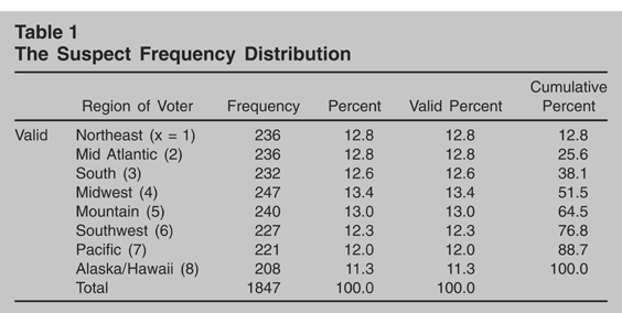
A week later, I received the students' problem sets, each of which included a frequency table for the region variable. To my surprise and initial consternation, 10 of the 30 students submitted problem sets with the frequency distribution presented in Table 1. How could 10 students using a random-number generator produce identical distributions? My immediate reaction was to suspect the students of colluding. I have experienced several cases of academic dishonesty that have made me, I regret to say, unnecessarily suspicious of the actions of students. Yet when I reviewed the 10 suspect submissions, something seemed amiss. Two students in particular caught my eye; they were figuratively and literally on opposite sides of the class. They seemed to be two unlikely conspirators, particularly with eight other students. There had to be another explanation. But what?
The Suspect Frequency Distribution

A more likely possibility occurred to me. Given the expense of purchasing individual licenses of SPSS, I know that most students use a campus computer laboratory with shared access to a copy of SPSS that resides on a university server. If the students were sharing a copy of the software, perhaps they shared a copy of the voter.sav dataset. I wondered: Might one student have created the “region” variable and saved it to the community copy of the dataset that resides on the server? If so, then it is plausible that students who subsequently worked on the exercise in the computer lab found that the dataset already had the region variable. Rather than re-creating the variable for the assignment, maybe the students simply generated a frequency table for the pre-existing variable. This would explain how 10 students produced identical distributions: they were all using the same data. To be sure, this violated the spirit of the assignment but did not rise to the level of malfeasance of mass copying. To me this scenario seemed much more likely than a student conspiracy.1
Due to the vagaries of software licensing and computer networks, I was unable to verify on my own whether the dataset on the server contained the suspect “region” variable. As a faculty member I log onto a different server and access a different version of SPSS than the students; without a student password and access to the student servers, I could not access the version of SPSS and the voter.sav dataset that students used. I thus relied on the college's technical support staff to help me verify students were not using a common dataset.
If the shared-variable explanation did not obtain, and if I discounted the possibility of cheating, what other explanations could there be? Is it possible that this was truly a random occurrence? To find out, I did a few quick calculations of probability. One can use the multinomial distribution to calculate the probability of any given student generating the frequency distribution in Table 1. As shown in the Appendix, the probability of a single student randomly generating the suspect frequency distribution is 2.5 × 10⁻¹², or about one in 400 billion (the odds of winning the Mega Millions lottery, by contrast, are a mere one in 176 million). If this is the probability of a single student generating this distribution, then it is highly improbable that 10 out of 30 students would obtain the same frequency distribution by chance. One can use the binomial distribution to calculate these long odds since the outcome is binary outcome (success is the distribution in Table 1, failure is all other possible frequency distributions) and the probability of success or failure is the same for each student (p = 2.5 × 10⁻¹²). The probability of 10 of my 30 students generating the same frequency distribution by chance is 3.3 × 10−109 (see Appendix). Thus I concluded it was highly improbable I was observing a chance event.
So where did that leave me? I didn't believe the students cheated. The university's servers prevent students from sharing a dataset. And the odds of this occurring by chance were so remote that I was confident it was not a fluke event. There seemed to be only one possible explanation left.
Reproducing Student Results
The only other possible explanation I could think of was that the SPSS software was doing something unexpected. Could it be that this popular and mature statistical software package does not generate random numbers? If so, perhaps I could replicate the suspect distribution that a third of the students produced. Though the answer key to the problem set that I previously had created included a different distribution, I nevertheless set out to see if I could reproduce the students' distribution.
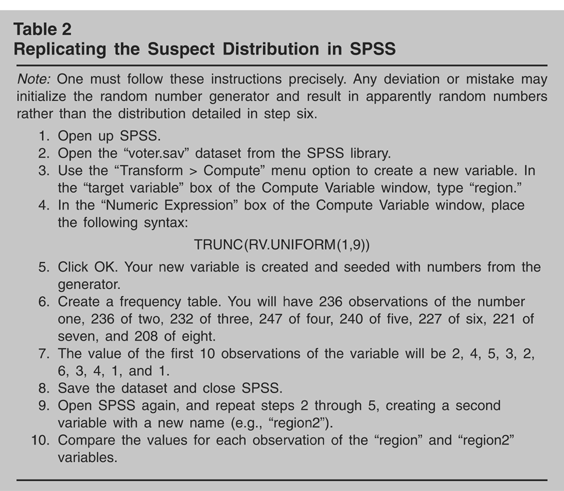
As my students did, I used the voter.sav dataset and followed my own step-by-step instructions. I created a “region” variable and used the conjoint syntax of the RV.UNIFORM() and TRUNC() functions to generate random discrete numbers between 1 and 8 for each of the dataset's observations. On my first attempt, I produced a distribution that differs from that of my students; SPSS appeared to be doing its job of producing random numbers. Confounded, I set aside the problem and returned to it an hour later. On my first attempt after this pause, however, I succeeded in producing the suspect distribution. I immediately tried again, but produced a different distribution. So what did I do differently so that I succeeded once in producing the apparently non-random distribution? The only difference I could think of was that I succeeded on my first attempt after setting aside the problem. Naturally, I exited SPSS on my computer in the intervening hour and then re-opened it when I returned to the problem. My first action in SPSS upon returning to the problem was to use the TRUNC(RV.UNIFORM()) syntax to generate the suspect random numbers. It appeared that my specific sequence of actions—opening the SPSS program, then immediately running the random number generator—gave rise to non-random numbers. I repeated this procedure of exiting SPSS, opening it, and immediately running the random number generator. Eureka! Each time I followed these specific steps, I created not only the suspect distribution but also an identical series of 1,847 discrete numbers. The “random” number generator produced perfectly predictable numbers. Table 2 shows the specific steps to follow to replicate the suspect distribution.
Replicating the Suspect Distribution in SPSS

This troubling finding raises two related questions. First, under what conditions does the random number generator in SPSS exhibit this behavior? Second, is the problem an idiosyncrasy of SPSS, or is it a problem of all statistical software? Tackling the first question, I wondered if the problem lay in the truncation function TRUNC() rather than in the RV.UNIFORM() function I was using. When I omitted the TRUNC() syntax and replicated the experiment, I was able to reproduce an identical series of continuous numbers when drawing from the uniform distribution. Likewise, I repeated the test drawing from other continuous distributions (the standard normal and Bernoulli with p = 0.5). Again I reproduced series of numbers that were identical for each distribution (though not across distributions—that is to say, the replicable series for the standard normal differed from the series generated by the Bernoulli). It appeared the random number generator exhibits this behavior when drawing from many distributions. But on further investigation, it appeared that SPSS produces non-random numbers only the first time the user invokes the random number generator. For each subsequent operation of the random functions in SPSS, the software produces apparently random numbers. So SPSS appears to produce reasonably random numbers, but only after the first call to the random number generator. I also noticed that if I made some mistake along the way—mistyped the syntax in the “Transform” dialogue window, for example—when I corrected the mistake, the resulting numbers appear random and non-replicable. This fact gave me an interesting insight into my students' problem sets. Those students who succeeded on the first try in creating the new variable and assigning values to it with the random number generator were the 10 students who produced the identical distribution. Ironically, only those students who made a couple of attempts produced apparently random distributions. The implication seems clear: the random number generator must be “initialized” somehow before it produces numbers that appear to be random. This behavior of the software appears to be fairly robust, furthermore. I found I could replicate the distribution in question on my first call to the random number generator even after conducting other operations in SPSS, such as generating a graph or running a regression.
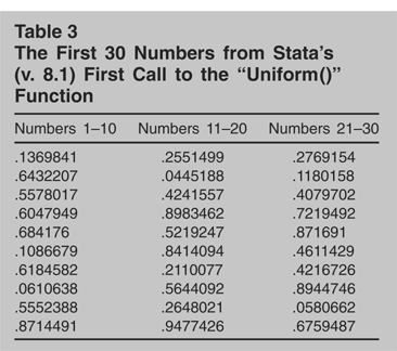
Is this behavior unique to SPSS's random number generator? Consider another statistics program. Given both Stata's popularity among political scientists (Beck 1995, 23–27; Altman and McDonald 2001, 683) and the fact that I own a license for version 8.1, I tried to reproduce the behavior in this software package (Stata for Windows v. 8.1, 2003). I replicated the conditions under which SPSS generated a perfectly predictable sequence of numbers: I created a new variable and seeded it using Stata's “uniform()” function, which draws random numbers from a uniform continuous distribution bounded by zero and one.2
The syntax in Stata is: gen VARNAME = uniform().
The First 30 Numbers from Stata's (v. 8.1) First Call to the “Uniform()” Function

It appears, then, that both Stata and SPSS require their respective random number generators to be initialized before they generate apparently random numbers. The fact that both of these programs exhibit this behavior suggests it is not a bug in any particular program. Unfortunately, the respective software vendors' web sites are of little help in explaining this feature. To the best of my ability, I found no information regarding the underlying algorithms each software uses to generate its random numbers; perhaps this is not a surprise given the proprietary nature of the softwares' algorithms. A quick survey of the relevant literature on “pseudo-random” number generators shows, however, a rich history of problems with using computers to generate random numbers (Sawitzki 1985; Park and Miller 1988; McCullough 1998, 363). As deterministic rule-driven beasts, computers cannot produce truly random numbers. To create pseudo-random numbers instead, software algorithms typically use a deterministic equation and “seed” it with some number to produce the pseudo-random number. To create variation in the seed, these pseudo-random generators may use a variable from somewhere in the computer's operating system—often the CPU's or server's clock, though software packages like SPSS and Stata also allow the user to set the seed's value at the outset of the generation process. Once the generator has created an initial pseudo-random number, it then uses this value as the seed for a subsequent number, and so on. Though different software packages may use different functions to create these pseudo-random numbers—according to Park and Miller (1988, 1193), Lehmer's function (1951) appears to be the most common—they all follow the principle of seeding subsequent calls to the function with the previously generated pseudo-random value. To create pseudo-random numbers drawn from other distributions (e.g., the normal and chi-square distributions), generators typically base their numbers on the uniform distribution (McCullough 1998, 364).
There is extensive documentation in the statistics and computer literature on the problems of generating random numbers in these ways (Park and Miller 1988; McCullough 1998; 1999) yet to my knowledge most discussions of statistical software in the political science literature barely address problems of pseudo-random number generators. This oversight becomes more problematic as political scientists adopt statistical software not only for pedagogical purposes, but also for increasingly popular Monte Carlo experiments. McCullough (1998, 363; 1999, 156) notes that although theoretical advances in computational sciences have kept pace with the demands of modern Monte Carlo experimentation, the opacity of software manufacturers' source code and the lack of documentation on their random number generators raises the question of whether current statistical software is adequately addressing problems of random number generation. This opacity is compounded by the absence of systematic testing of the random numbers generated by popular statistical software packages. For example, a recent review of statistical programs tested the accuracy of several software packages' descriptive statistics, ANOVA tests, linear and nonlinear regression algorithms, and their distributions, but not their random number generators (Altman and McDonald 2001). This is not a trivial oversight: McCullough (1999) finds non-randomness in the generators in SPSS, SAS, and S-Plus.
I should make clear that I intend none of this to be a criticism of SPSS. As it turns out, the software's programmers intend the program to behave this way for reasons I discuss shortly. I suspect, however, that most political scientists are like me. They are unfamiliar with how the statistical software works and impart an understanding of “randomness” to these numbers that is not what the manufacturers and code-writers intend. The answer to why my students produced “non-random” numbers lies in the distinction between randomness and non-reproducibility. Recall that my students' exercises produced apparently non-random numbers with the initial call to the random number generator after starting SPSS. This arises because the seed value for the random number generator is fixed at the time of starting both SPSS and Stata. So each and every time one starts the software, the random-number generator begins with the same value and produces a series of numbers drawn from a known distribution using a fixed rule. Hence the “random” numbers are perfectly reproducible.
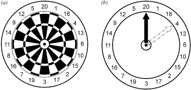
Typically students (and I) think of “random” numbers, however, as those that arise due to chance occurrences. Because these chance occurrences are themselves unique, we think one can never reproduce a series of random numbers. Consider the difference between a dartboard and a clock. Students, and perhaps many political scientists, think of random number generation as the equivalent to throwing a dart. For unknowable reasons of chance and fortune—perhaps a tremor in one's hand, or a draft—the dart ultimately finds one unique value. Repeated throws will produce a random sequence of numbers, thanks to our human failings and the vicissitudes of nature. Even the steadiest among us cannot reproduce a sequence on a dartboard. This is how students and, until recently, I thought about random number generation. We think statistical software engages in some sort of dart-throwing exercise, in which chance plays an essential role in the selection of “random” numbers. In fact, the process computers use is more like the sweep of a hand across the face of a clock. Suppose one affixed a hand to the face of a dartboard (see Figure 1). The hand would proceed across the face of the dartboard in clockwise fashion, resting on each of the 20 values before ticking onward. If we add some simple rule for taking a value based on the position of the clock hand, we could generate a sequence of apparently random numbers that nevertheless is perfectly replicable. For example, we could take every third tick of the clock hand starting from the noon position. This would give us the following string of discrete values: 4, 10, 17, 7, 11, 12, 1, 13, 15, 3 … and so on. The numbers are “random” in the sense that the placement of values on the dartboard is random (Cohen and Tonkes 2001). But the rule used to select from among these random values is deterministic, and hence perfectly replicable. Each and every time we take the third tick of the clock hand across the dartboard starting from the noon position, we will produce the same sequence of random numbers.

Random Number Generation on a Dartboard: Darts (a) versus a Clock Hand (b)
I now like to think of random number generation in terms of a table of random numbers from an old statistics text (e.g., Mason et al. 1994, A-14–A-16). Many of us first learned to select random numbers from such tables. Suppose one selected random numbers from such a table using a simple rule (“take the first number in every third line” or “use every 43rd number”). Though the numbers in the table are random, if one were to follow the same rule every time using the same table, one would reproduce the same series of numbers. While the numbers are “random” in the sense that they are drawn from a known distribution, the selection process is not at all random. In this respect, the term “generator” is a pernicious misnomer for how popular statistics programs work. Rather than “generating” random numbers by throwing a dart and hoping for a gust of wind, they are marching like a second hand across the face of a clock whose numbers are scrambled.
This process of selecting pseudo-random numbers in SPSS and Stata is opaque. Both packages include documentation that specifies their initial random number seeds are fixed (see SPSS 11.0 Syntax Reference Guide 2001, 1132).3
The Stata user can create a brief macro that will initialize the program's random number generator with the CPU's clock, thus varying the starting point for the generation of a series of random numbers. The syntax is:

This syntax creates a six-digit integer to seed the generator based on the time value of the computer's internal clock. A user who typed this syntax at 5:13:39 in the afternoon would produce the seed value of 171339 (since the internal clock is a 24-hour variety). I thank Yulia Marchenko at Stata Technical Support for sharing this code with me.
This is true both of the active generator and the Mersenne Twister. The problem appears to be that SPSS does not retain the initialization of the active generator between each session. Following the same procedures outlined in this paper, I was able to again reproduce an identical series of numbers. This suggests that, although the SPSS documentation indicates that the starting point for the active generator is a randomly selected number, in fact it too is a fixed value—albeit one that differs from the default starting seed of 2,000,000. For users of SPSS v. 13.0 or v.14.0 who wish to verify this, using the TRUNC(RV.UNIFORM(1,9)) syntax the active number generator produces the following sequence: 3, 1, 1, 1, 5, 7, 6, 6, 8, 6, 7, 2, 6, 4, 1 ….
Conclusions
Needless to say, my students and I learned much more from this simple SPSS exercise than we had anticipated. In our next class session, I took a few minutes to illustrate the reproducibility of pseudo-random numbers in SPSS. My undergraduates quickly understood the nature of the problem, even if they were somewhat puzzled by my interest in it. I take three lessons away from this exercise that I hope to impart to both my students and my colleagues. First, we should meticulously refer to “pseudo-random” numbers in our instruction and research, because the computer-based processes that we use to select such numbers are decidedly deterministic (e.g., Farkas 1996, fn. 19; Gordon 2002, 207). We need to make sure that both we and our students are thinking of the sweep of a clock hand rather than the flight of a dart. Second, when using statistical software we should know what seed values the package uses to start the selection of random numbers. If the starting seed is a fixed integer, we should manually alter the starting seed for each generation in order to create some variability in the starting point for the series of numbers. Software that allows variation in the starting seed is desirable, and we should ensure we select this option whenever our instructional or research task allows it (Cusack and Stoll 1994, 45). If the reproduction of random numbers is necessary for replication and verification of results either of student exercises or of our own research, we should make explicit the seed values we use (as do Farkas 1996; and Gordon 2002). Otherwise, we may run the risk of gathering a “random” sample that is anything but randomly selected (see Drury 2001, 497) or that corrects for one kind of sampling bias with another bias that is much less apparent (Reiter and Stam 1998, fn. 10). Finally, when we use statistical software in the classroom, we must understand and explain how it works. In my case, the reproducibility of pseudo-random numbers gave me the false impression that my students had cheated. Fortunately, common sense prevented me from imposing any sanctions. But the experience was sobering. If my undergraduate students, who were novice SPSS users, could create replicable “random” numbers, how many times had I unwittingly conducted “random” number generation that is anything but?
Biography
David C. Earnest is assistant professor of political science and international studies at Old Dominion University, Norfolk, VA. His substantive research focuses on the political incorporation of migrants in democratic societies, while his methodology interests are in the application of agent-based models to problems of domestic and international politics. At ODU, Earnest teaches courses in international political economy, international relations theory, and political methodology. He is co-author (with James N. Rosenau, Yale H. Ferguson, and Ole R. Holsti) of On the Cutting Edge of Globalization: An Inquiry into American Elites (Rowman & Littlefield, 2005).