





1. Introduction
Despite over half a century of research and several review articles (e.g. Turner Reference Turner1986; Fernando Reference Fernando1991; Woods Reference Woods2010; de Rooy Reference de Rooy, Bechtold, Fröhlich, Hohenegger, Jonker, Mironov, Siebesma, Teixeira and Yano2013; Da Silva et al. Reference Da Silva, Hunt, Eames and Westerweel2014; Mellado Reference Mellado2017), our understanding of turbulent entrainment (the transport of fluid from regions of relatively low to relatively high levels of turbulence) remains fragmented. One important reason is that turbulent entrainment is notoriously difficult to determine. Entrainment is a process that typically occurs over much larger time scales than turbulent time scales, and its effects are therefore easily obfuscated by turbulent fluctuations and transient effects. Furthermore, the quantification of turbulent entrainment requires the determination of a turbulent and non-turbulent (or less turbulent) region which is, by definition, arbitrary and thus subject to uncertainty.
However, there are other reasons that the understanding of turbulent entrainment remains challenging. One challenge is the sheer number of flows in which turbulent entrainment plays a role. Developing boundary layers can be classified based on the number of independent variables on which their solution depends, with a further distinction between statistically steady and unsteady problems, as shown in table 1. Consider a turbulent velocity field  $\boldsymbol {u}(x,y,z,t)$, which will generally not have any symmetries. By ensemble averaging this velocity field, denoted by
 $\bar {\cdot }$, an average velocity field
 $\bar {\boldsymbol {u}}$ is obtained which satisfies the symmetries present in the problem formulation (such as axisymmetric or streamwise homogeneity). In table 1,
 $x$ is the (slowly developing) streamwise direction, and
 $z$ or
 $r$ is the normal direction, where
 $z$ would be used for planar problems and
 $r$ for axisymmetric problems. Free-shear flows require a minimum of two inhomogeneous directions. The class of steady problems with two independent variables comprises e.g. planar and axisymmetric jets (Hussein, Capp & George Reference Hussein, Capp and George1994; Da Silva & Métais Reference Da Silva and Métais2002; Westerweel et al. Reference Westerweel, Fukushima, Pedersen and Hunt2005; Watanabe et al. Reference Watanabe, Sakai, Nagata, Ito and Hayase2014), plumes (List Reference List1982), wakes (Cantwell & Coles Reference Cantwell and Coles1983; Obligado, Dairay & Vassilicos Reference Obligado, Dairay and Vassilicos2016), fountains (Hunt & Burridge Reference Hunt and Burridge2015), boundary layers (Head Reference Head1958; Sillero, Jimenez & Moser Reference Sillero, Jimenez and Moser2013), mixing layers (Rajaratnam Reference Rajaratnam1976) and inclined gravity currents (Wells, Cenedese & Caulfield Reference Wells, Cenedese and Caulfield2010; Odier, Chen & Ecke Reference Odier, Chen and Ecke2014; Krug et al. Reference Krug, Holzner, Luethi, Wolf, Kinzelbach and Tsinober2015).
Classification of free-shear flows based on the number of independent variables.

In the class of unsteady problems with two independent variables are problems that develop slowly in time in one spatial dimension,  $z$ or
 $r$. These are problems such as penetrative convection (Mellado Reference Mellado2012; Holzner & van Reeuwijk Reference Holzner and van Reeuwijk2017), convective and stable boundary layers (as relevant to the atmospheric boundary layer and the oceanic mixed layer; Kato & Phillips Reference Kato and Phillips1969; Deardorff, Willis & Stockton Reference Deardorff, Willis and Stockton1980; Sullivan et al. Reference Sullivan, Moeng, Stevens, Lenschow and Mayor1998; Jonker et al. Reference Jonker, Van Reeuwijk, Sullivan and Patton2013; Garcia & Mellado Reference Garcia and Mellado2014), stratocumulus clouds (Mellado Reference Mellado2017), but also include temporal jets (Da Silva & Pereira Reference Da Silva and Pereira2008; van Reeuwijk & Holzner Reference van Reeuwijk and Holzner2014), plumes (Krug et al. Reference Krug, Chung, Philip and Marusic2017), gravity currents (van Reeuwijk, Krug & Holzner Reference van Reeuwijk, Krug and Holzner2018; van Reeuwijk, Holzner & Caulfield Reference van Reeuwijk, Holzner and Caulfield2019), wakes (Redford, Castro & Coleman Reference Redford, Castro and Coleman2012; Watanabe et al. Reference Watanabe, Riley, De Bruyn Kops, Diamessis and Zhou2016), mixing layers (Watanabe et al. Reference Watanabe, Riley, Nagata, Onishi and Matsuda2018a) and compressible reacting mixing layers (Jahanbakhshi & Madnia Reference Jahanbakhshi and Madnia2018). These temporal flows are not generally encountered in nature but share many of the features of their two-dimensional (2-D) steady cousins. However, with two homogeneous spatial directions, they are ideal for exploration with direct numerical simulation.
Steady problems with three independent variables possess two normal directions in which the flow develops ‘fast’ but in an anisotropic manner. Examples are jets and plumes discharged vertically in a cross-wind (Mahesh Reference Mahesh2013; De Wit, Van Rhee & Keetels Reference De Wit, Van Rhee and Keetels2014; Woods Reference Woods2010; Devenish, Rooney & Thomson Reference Devenish, Rooney and Thomson2010), stratified wakes (Xu, Fernando & Boyer Reference Xu, Fernando and Boyer1995) and horizontally discharged point releases in stratified fluid layers. The class of unsteady problems with three independent variables comprises all the flows mentioned in the category of 2-D steady developing boundary layers, provided that one of their boundary conditions or the environment changes in time. Examples include unsteady jets and plumes (Scase et al. Reference Scase, Caulfield, Dalziel and Hunt2006; Craske & van Reeuwijk Reference Craske and van Reeuwijk2015, Reference Craske and van Reeuwijk2016; Woodhouse, Phillips & Hogg Reference Woodhouse, Phillips and Hogg2016) and starting plumes (Turner Reference Turner1962). The class of unsteady problems with four independent variables comprises unsteady versions in the category of 3-D steady free-shear flows. These comprise unsteady gravity currents from a point source, and unsteady jets/plumes in a cross-flow.
Turbulent entrainment is generally studied either from a local or a global perspective. The global approach involves inferring the entrainment velocity from the Reynolds-averaged equations (e.g. Townsend Reference Townsend1976; Turner Reference Turner1986) and considers entrainment from an integral perspective. The local approach, as pioneered by Corrsin & Kistler (Reference Corrsin and Kistler1955), considers the microscale perspective. The local approach starts from choosing a scalar quantity  $\chi$ to provide an implicit definition of the instantaneous turbulent–non-turbulent interface (TNTI), where a threshold value
 $\chi _0$ is used to distinguish the turbulent zone (
 $\chi \geqslant \chi _0$) from the non-turbulent zone (
 $\chi <\chi _0$). The most commonly used scalar quantity is enstrophy (e.g. Bisset, Hunt & Rogers Reference Bisset, Hunt and Rogers2002; Holzner & Luethi Reference Holzner and Luethi2011; Da Silva et al. Reference Da Silva, Hunt, Eames and Westerweel2014; van Reeuwijk & Holzner Reference van Reeuwijk and Holzner2014), which is consistent with Corrsin & Kistler (Reference Corrsin and Kistler1955), but passive scalars (e.g. Sreenivasan, Ramshankar & Meneveau Reference Sreenivasan, Ramshankar and Meneveau1989; Westerweel et al. Reference Westerweel, Fukushima, Pedersen and Hunt2005; Burridge et al. Reference Burridge, Parker, Kruger, Partridge and Linden2017) or the turbulence kinetic energy (Chauhan et al. Reference Chauhan, Philip, de Silva, Hutchins and Marusic2014; Philip et al. Reference Philip, Meneveau, de Silva and Marusic2014) are also used to define the TNTI. Note, however, that care needs to be taken when using turbulence kinetic energy to delineate the TNTI, as pressure can induce irrotational velocity fluctuations in the ambient (Watanabe, Zhang & Nagata Reference Watanabe, Zhang and Nagata2018b).
The choice of the threshold value  $\chi _0$ is always slightly arbitrary, as the flow transitions smoothly from turbulent to non-turbulent. In addition any measurement and simulation data are subject to uncertainty, and background levels of
 $\chi$ may be non-zero (e.g. enstrophy levels in a turbulent ambient). One therefore typically chooses a small and finite non-zero threshold
 $\chi _0$ to define the TNTI. Since the interface between turbulent and non-turbulent fluid is generally very sharp, there is a range of thresholds
 $\chi _0$ that can be chosen for which the entrainment statistics are insensitive to the choice of
 $\chi _0$ (Da Silva et al. Reference Da Silva, Hunt, Eames and Westerweel2014).
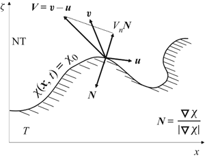
The velocity  ${\boldsymbol {v}}$ associated with any trajectory on an isosurface of
 $\chi$ satisfies
 \begin{equation} \frac{{\mathrm{d}} \chi}{{\mathrm{d}} t} = \frac{\partial \chi}{\partial t} + \boldsymbol{v} \boldsymbol{\cdot} \boldsymbol{\nabla}\chi = 0. \end{equation}
By introducing a relative velocity  $\boldsymbol {V} = \boldsymbol {v} - \boldsymbol {u}$, which is the difference between the isosurface velocity
 $\boldsymbol {v}$ and the fluid velocity
 $\boldsymbol {u}$, (1.1) can be rewritten as (Dopazo, Martín & Hierro Reference Dopazo, Martín and Hierro2007; Holzner & Luethi Reference Holzner and Luethi2011)
 \begin{equation} V_n = - \frac{1}{| \boldsymbol{\nabla} \chi |} \frac{\textrm{D} \chi}{\textrm{D} t}, \end{equation}
where  $\textrm {D}/\textrm {D}t=\partial /\partial t + \boldsymbol {u} \boldsymbol {\cdot } \boldsymbol {\nabla }$ is the material derivative,
 $V_n = \boldsymbol {V} \boldsymbol {\cdot } \boldsymbol {N}$ is the normal component of the relative velocity and
 $\boldsymbol {N}=\boldsymbol {\nabla } \chi / | \boldsymbol {\nabla } \chi |$ is the (3-D) normal vector pointing into the turbulent region (figure 1a). Note that the other two components of
 $\boldsymbol {V}$ tangential to the isosurface are not specified by this definition. For an entraining flow,
 $V_n<0$, which is a consequence of defining a normal
 $\boldsymbol {N}$ that points into
 $\varOmega$. The inward pointing normal also has consequences for the Gauss divergence theorem. By substituting the governing equation for
 $\chi$ (usually enstrophy) into (1.2) and averaging, local aspects of turbulent entrainment can be explored (e.g. Holzner & Luethi Reference Holzner and Luethi2011; Da Silva et al. Reference Da Silva, Hunt, Eames and Westerweel2014; van Reeuwijk & Holzner Reference van Reeuwijk and Holzner2014; Krug et al. Reference Krug, Holzner, Luethi, Wolf, Kinzelbach and Tsinober2015; Jahanbakhshi & Madnia Reference Jahanbakhshi and Madnia2018).
Interface properties of the turbulent–non-turbulent interface separating turbulent ( $T$) from non-turbulent (NT) fluid. (a) Definition sketch. (b) Geometric properties.

The global entrainment velocity  $\bar {V}_g$ is not as uniquely defined as the local entrainment velocity (1.2) (Hunt, Rottman & Britter Reference Hunt, Rottman and Britter1983; Turner Reference Turner1986). For spatially developing flows, the entrainment velocity is usually associated with a flow into the turbulent region. For temporal problems, however, it is defined via
 ${\mathrm {d}} h / {\mathrm {d}} t$, the growth of the layer in time, where
 $h$ is some characteristic layer thickness. For spatially developing flows in which the environment is non-quiescent or is stratified, there is another mode of entrainment which is associated with the entrainment across the boundary. These different forms of entrainment were discussed in Hunt et al. (Reference Hunt, Rottman and Britter1983) and Turner (Reference Turner1986) and cause confusion between disciplines, as they describe related processes that are not necessarily equivalent. In this paper we derive an unambiguous definition of the global entrainment velocity that can be used for spatial, temporal and spatio-temporal (unsteady) entrainment problems.
The aim of this paper is to derive an integral description of free-shear flows capable of representing both the local and global viewpoints of turbulent entrainment. An equivalent definition to (1.2) is presented for the global entrainment velocity. The framework provides a unified description of entrainment in temporal problems (2-D unsteady; Da Silva & Pereira Reference Da Silva and Pereira2008; van Reeuwijk & Holzner Reference van Reeuwijk and Holzner2014; Krug et al. Reference Krug, Chung, Philip and Marusic2017), in which the TNTI moves but there is no net flow into the turbulent layer ( $V_n$ produced by
 $\boldsymbol {v}$), spatial problems (2-D steady; Rajaratnam Reference Rajaratnam1976; Turner Reference Turner1986; Philip et al. Reference Philip, Meneveau, de Silva and Marusic2014), in which the TNTI is statistically steady but there is a net flow into the turbulent layer (
 $V_n$ produced by
 $\boldsymbol {u}$), and unsteady free-shear layers (3-D unsteady; Craske & van Reeuwijk Reference Craske and van Reeuwijk2016).
This paper is organised as follows. Section 2 introduces the integral operator identities and the averaged plane-integrated Navier–Stokes equations which describe the integral spatio-temporal dynamics of free-shear flows. In § 3, an average isosurface of  $\bar {\chi }$ is applied to the equations which results in an expression for the global entrainment velocity
 $\bar {V}_g$ in terms of an explicit function
 $h_t$ describing the TNTI. The implications of this new definition of
 $\bar {V}_g$ are discussed in § 4. Four canonical free-shear flows (an axisymmetric jet, a planar wake, a temporal jet and an unsteady jet/plume) are studied in § 5 to show that the current definition of
 $\bar {V}_g$ is fully consistent with previous results. Application of the new description to unsteady jets and plumes reveals the relation between the entrainment coefficient
 $\alpha$ and actual entrainment across the interface. Concluding remarks are made in § 6.
2. Local averaged integral equations
In this section we present integral volume (i.e. continuity) and momentum conservation equations. The focus of this work is on turbulent free-shear flows which develop slowly (in a statistical sense) in time  $t$, in the spatial direction
 $x$ or both. The incompressible Navier–Stokes equations are given by
 \begin{gather} \boldsymbol{\nabla}\boldsymbol{\cdot} \boldsymbol{u} =0, \end{gather}
 \begin{gather}\frac{\textrm{D} \boldsymbol{u}}{\textrm{D} t} = - \frac{1}{\rho_0} \boldsymbol{\nabla} p + \boldsymbol{\nabla}\boldsymbol{\cdot}\boldsymbol{\mathsf{T}} + \boldsymbol{f}, \end{gather}
where  $\boldsymbol{\mathsf{T}}$ denotes the viscous stress tensor and
 $\boldsymbol {f}$ is a body force. These equations will be integrated over the turbulent region in the
 $y$–
 $z$ plane which is denoted
 $\varOmega$. The following identities for the integrals of the gradient, divergence and material derivative operators can be derived:
 \begin{gather} \int_{\varOmega} \boldsymbol{\nabla} \phi \,{\mathrm{d}} A = \frac{\partial}{\partial x} \int_{\varOmega} \phi \,{\mathrm{d}} A \boldsymbol{e}_x - \oint_{\partial \varOmega} \phi \frac{\boldsymbol{N}}{| \boldsymbol{N}_\perp|} \,{\mathrm{d}} \ell, \end{gather}
 \begin{gather}\int_{\varOmega} \boldsymbol{\nabla}\boldsymbol{\cdot} \boldsymbol{F} \,{\mathrm{d}} A = \frac{\partial}{\partial x}\int_{\varOmega} F_x \,{\mathrm{d}} A- \oint_{\partial \varOmega} \boldsymbol{F} \boldsymbol{\cdot} \frac{\boldsymbol{N}}{| \boldsymbol{N}_\perp|} \,{\mathrm{d}} \ell, \end{gather}
 \begin{gather}\int_{\varOmega} \frac{\textrm{D} \phi}{\textrm{D} t} \,{\mathrm{d}} A = \frac{\partial }{\partial t}\int_{\varOmega} \phi \, {\mathrm{d}} A + \frac{\partial}{\partial x} \int_{\varOmega} u_x \phi \, {\mathrm{d}} A - \int_{\varOmega} \phi \boldsymbol{\nabla}\boldsymbol{\cdot} \boldsymbol{u} \,{\mathrm{d}} A + \oint_{\partial \varOmega} \frac{V_n}{| \boldsymbol{N}_\perp|} \phi \, {\mathrm{d}} \ell, \end{gather}
where  $\phi$ is an arbitrary scalar or vector component field and
 $\boldsymbol {F}$ is an arbitrary vector field. Vectors with a perp (
 $\perp$) subscript denote the components perpendicular to the
 $x$-direction, i.e.
 $\boldsymbol {F} =[F_x, \boldsymbol {F}_\perp ]^\textrm {T}$, and
 $\boldsymbol {\nabla }_\perp =[\partial /\partial y, \partial / \partial z]^\textrm {T}$. The unit vector
 $\boldsymbol {N}=\boldsymbol {\nabla } \chi / | \boldsymbol {\nabla } \chi |$ is normal to the 3-D surface
 $\chi = \chi _0$ which demarcates between turbulent and non-turbulent regions. The normal vector can be written as
 $\boldsymbol {N} = [N_x, \boldsymbol {N}_\perp ]^\textrm {T}$, so that
 $|\boldsymbol {N}_\perp |$ is the magnitude of the 3-D normal in the
 $y$–
 $z$ plane (see figure 1b). Finally,
 ${\boldsymbol {e}}_x$ is the unit vector in the
 $x$-direction and
 $u_x$ is the component of the fluid velocity field
 $\boldsymbol {u}$ in that same direction. An easily accessible yet rigorous proof of these three identities is given in appendix A. A more general derivation using differential geometry, which highlights the role of Stokes’ theorem and the Leibniz integral rule, is given in appendix B.
Since the flow is turbulent, the integration domain  $\varOmega (y,z;x)$ can consist of several disconnected blobs of turbulent fluid, i.e.
 $\varOmega = \varOmega _1 \cup \varOmega _2 \cup \ldots$. This implies that the domain boundary
 $\partial \varOmega$ contains multiple closed trajectories
 $\partial \varOmega _1, \partial \varOmega _2, \ldots$ which are summed up with the line integral, That is,
 $\oint _{\partial \varOmega }\cdot \,{\mathrm {d}} \ell =\oint _{\partial \varOmega _1}\cdot \,{\mathrm {d}} \ell +\oint _{\partial \varOmega _2}\cdot \,{\mathrm {d}} \ell +\ldots$ if the domain contains multiple disconnected blobs.
Noting that  $\boldsymbol {\nabla }\boldsymbol {\cdot } \boldsymbol {u} = \textrm {D}\phi /\textrm {D} t=0$ for
 $\phi = 1$ and using (2.5) implies that the instantaneous integral continuity equation is given by
 \begin{equation} \frac{\partial}{\partial t} \int_{\varOmega} \,{\mathrm{d}} A + \frac{\partial}{\partial x} \int_{\varOmega} u_x \, {\mathrm{d}} A = -\oint_{\partial \varOmega} \frac{V_n}{| \boldsymbol{N}_\perp|} \, {\mathrm{d}} \ell . \end{equation}
Note that if the relative isosurface velocity  $\boldsymbol {V}$ is everywhere tangential to the interface then
 $V_n=0$, in which case (2.6) describes a streamtube. Entrainment allows exchange across the isosurface
 $\chi =\chi _0$. For an entraining flow,
 $V_n<0$ (due to the inward pointing normal).
The line integral represents the net entrainment into the turbulent region. The factor  $|\boldsymbol {N}_\perp |$ accounts for the projection of the 3-D quantity
 $V_n$ onto the
 $y$–
 $z$ plane. This is better seen by using
 $V_n = \boldsymbol {V} \boldsymbol {\cdot } \boldsymbol {N}$ to write the entrainment term as
 \begin{equation} \oint_{\partial \varOmega} \frac{V_n}{| \boldsymbol{N}_\perp|} \, {\mathrm{d}} \ell = \oint_{\partial \varOmega} \boldsymbol{V}_\perp \boldsymbol{\cdot} \boldsymbol{n}\, {\mathrm{d}} \ell + \oint_{\partial \varOmega} V_x\frac{N_x}{| \boldsymbol{N}_\perp|} \, {\mathrm{d}} \ell, \end{equation}
where  $\boldsymbol {n} = \boldsymbol {\nabla }_\perp \chi /|\boldsymbol {\nabla }_\perp \chi |$ is the normal in the
 $y$–
 $z$ plane, and note that this quantity is related to the 3-D normal via
 $\boldsymbol {n} = \boldsymbol {N}_\perp / |\boldsymbol {N}_\perp |$. The first term on the right-hand side of (2.7) is simply the entrainment flux arising from the in-plane relative velocity components
 $\boldsymbol {V}_\perp$. As described in appendices A and B, the second term on the right-hand side of (2.7) arises from the commutation of integration and differentiation with respect to
 $x$ that is required to formulate (2.6). It represents the net transport of the streamwise relative velocity component
 $V_x$ into the turbulent region across the interface whose local slope is
 $N_x/|\boldsymbol {N}_\perp |$ (see figure 1). We note that
 $|\boldsymbol {N}_\perp |$ can be zero locally when
 $\boldsymbol {N}$ is aligned with the
 $x$-direction , which would render the integrand infinite. This is an inescapable consequence of determining entrainment as a function of
 $x$. Any subsequent integration over
 $x$ will remain finite, however, since
 $V_n/ | \boldsymbol {N}_\perp | \,{\mathrm {d}} \ell \,\textrm {d}x =V_n \,{\mathrm {d}} S$ where
 ${\mathrm {d}} S$ is the local surface area of the surface in three dimensions.
Integration over the region  $\varOmega$ of (2.2) and use of identities (2.3)–(2.5) results in
 \begin{align} &\frac{\partial}{\partial t} \int_{\varOmega} \boldsymbol{u} \, {\mathrm{d}} A + \frac{\partial}{\partial x} \int_{\varOmega} \left(u_x \boldsymbol{u} +\frac{p}{\rho_0} \boldsymbol{e}_x\right) {\mathrm{d}} A \nonumber\\ &\quad =- \oint_{\partial \varOmega} \frac{1}{| \boldsymbol{N}_\perp|} \left( V_{n} \boldsymbol{u} - \frac{p}{\rho_0} \boldsymbol{N}\right) {\mathrm{d}} \ell + \int_{\varOmega} \boldsymbol{f}\, {\mathrm{d}} A. \end{align}
Here, the shear-stress contributions have been neglected as is conventional for high Reynolds free-shear flows. Equations (2.6) and (2.8) are instantaneous.
Performing ensemble averaging, denoted by the overbar  $\overline {\cdot }$, on the instantaneous integrated continuity (2.6) and the streamwise
 $x$-component of the integrated momentum (2.8) yields
 \begin{equation} \frac{\partial}{\partial t} {\overline{\int_{\varOmega} \, {\mathrm{d}} A}} + \frac{\partial}{\partial x} \overline{\int_{\varOmega} u_x \, {\mathrm{d}} A } = -\overline{\oint_{\partial \varOmega} \frac{V_{n}}{|\boldsymbol{N}_\perp|} \, {\mathrm{d}} \ell}, \\ \end{equation}
 \begin{align} &\frac{\partial}{\partial t} \overline{\int_{\varOmega} u_x \, {\mathrm{d}} A} + \frac{\partial}{\partial x} \overline{\int_{\varOmega} \left(u_x^2 + \frac{p}{\rho_0}\right) {\mathrm{d}} A} \nonumber\\ &\quad =- \overline{\oint_{\partial \varOmega} \frac{1}{| \boldsymbol{N}_\perp|} \left( V_{n} u_x - \frac{p}{\rho_0} N_x \right) {\mathrm{d}} \ell} + \overline{\int_{\varOmega} f_x \,{\mathrm{d}} A}. \end{align}
In the integral continuity (2.9),  $\overline {\int _{\varOmega } \,{\mathrm {d}} A}$ represents the average instantaneous cross-sectional area of the turbulent region at location
 $x$. It is not possible to commute the integral with the ensemble averaging because the integration regions
 $\varOmega$ and
 $\partial \varOmega$ vary in time and per ensemble instance.
3. Global averaged integral equations
Equations (2.9), (2.10) ultimately link the integral behaviour of the free-shear flow to the small-scale dynamics at the TNTI when  $\chi$ is an instantaneous quantity. The global, integral dynamics can be obtained by using an average quantity
 $\bar {\chi }$, with associated threshold
 $\bar {\chi }_0$, to identify the interface (figure 2). By considering an average quantity, the TNTI will not be contorted but will be smooth and satisfy the symmetries corresponding to homogeneity in the problem under consideration.
Definition sketch of the global (average) perspective on the turbulent–non-turbulent interface.

3.1. Non-slender flows
We define the global entrainment velocity  $\bar {V}_g$ to be the net transport across an averaged scalar
 $\bar {\chi }$. This implies that the 3-D normal is defined as
 $\boldsymbol {N}_g = \boldsymbol {\nabla } \bar \chi / | \boldsymbol {\nabla } \bar \chi |$, and therefore that
 \begin{equation} V_g = ({\boldsymbol{v}}-{\boldsymbol{u}}) \boldsymbol{\cdot} {\boldsymbol{N}}_g = \frac{{\boldsymbol{v}} \boldsymbol{\cdot} \boldsymbol{\nabla} \bar \chi - {\boldsymbol{u}} \boldsymbol{\cdot} \boldsymbol{\nabla} \bar \chi}{|\boldsymbol{\nabla} \bar \chi|} = - \frac{1}{|\boldsymbol{\nabla} \bar \chi|} \frac{ \textrm{D} \bar \chi}{ \textrm{D} t}, \end{equation}
where use was made of (1.1) for  $\chi = \bar \chi$. The equation above is the instantaneous global entrainment velocity across an isosurface based on a Reynolds-averaged quantity. The mean entrainment velocity can be determined by applying Reynolds averaging to (3.1), with result
 \begin{equation} \bar{V}_g = \overline{\boldsymbol{V} \boldsymbol{\cdot} \boldsymbol{N}_g} = \bar{\boldsymbol{V}} \boldsymbol{\cdot} \boldsymbol{N}_g = - \frac{1}{|\boldsymbol{\nabla} \bar \chi|} \frac{\bar{\textrm{D}} \bar \chi}{\bar{\textrm{D}} t}, \end{equation}
where  $\bar {\textrm {D}}/\bar {\textrm {D}}t = \partial /\partial t + \bar {\boldsymbol {u}} \boldsymbol {\cdot } \boldsymbol {\nabla }$ is the material derivative of the average flow.
An advantage of considering averaged quantities is that it is possible to represent the isosurface  $\bar {\chi }=\bar {\chi }_0$ (which implicitly defines the TNTI) explicitly in terms of a single-valued function
 $h_t$ in a coordinate system appropriately representing the symmetries of the free-shear problem under consideration. Restricting attention to planar or axisymmetric problems, a scalar level-set function
 $L(x,\zeta ,t) = h_t(x, t) - \zeta$ can be constructed such that
 $L=0$ represents the average interface position where
 $\zeta$ is the direction normal to the x-direction. Setting
 $\bar {\chi } = L$ implies that (3.1) can equivalently be expressed as
 \begin{equation} \bar{V}_g = -\frac{1}{|\boldsymbol{\nabla} L |} \left( \frac{\bar{ \textrm{D}} h_t}{\bar{\textrm{D}} t} - \frac{\bar{ \textrm{D}} \zeta}{\bar{\textrm{D}} t}\right) = \frac{1}{| \boldsymbol{\nabla} L |} \left( \bar{u}_\zeta - \frac{\bar {\textrm{D}} h_t}{\bar {\textrm{D}} t} \right), \end{equation}
where  $|\boldsymbol {\nabla } L| = \sqrt {1 + (\partial h_t / \partial x)^2}$.
Because the interface is based on the average quantity  $\bar {\chi }$, the averaging and integral operators do commute, which implies that (2.9), (2.10) simplify to
 \begin{equation} \frac{\partial}{\partial t} {\int_{\bar{\varOmega}} \,{\mathrm{d}} A} + \frac{\partial}{\partial x} \int_{\bar{\varOmega}} \bar{u}_x \, {\mathrm{d}} A = -\oint_{\partial \bar{\varOmega}} \frac{\bar{V}_{g}}{|\boldsymbol{N}_{g\perp}|} \, {\mathrm{d}} \ell, \end{equation}
 \begin{align} &\frac{\partial}{\partial t} \int_{\bar{\varOmega}} \bar{u}_x \, {\mathrm{d}} A + \frac{\partial}{\partial x} \int_{\bar{\varOmega}} \left(\overline{u_x^2} + \frac{\bar{p}}{\rho_0} \right) {\mathrm{d}} A \nonumber\\ &\quad = - \oint_{\partial \bar{\varOmega}} \frac{1}{| \boldsymbol{N}_{g\perp}|} \left( \overline{V_{g} u_x} - \frac{\bar{p}}{\rho_0} N_{gx} \right) {\mathrm{d}} \ell + \int_{\bar{\varOmega}} \bar{f}_x \,{\mathrm{d}} A. \end{align}
Here, we have denoted the integration domain and boundary with  $\bar {\varOmega }$ and
 $\partial \bar {\varOmega }$, respectively, to distinguish from the local viewpoint. The integrals can be made definite once a specific coordinate system is selected. Note that
 $\overline {u_x^2}=\bar {u}_x^2 + \overline {u'_x u'_x}$.
3.2. Slender flows
Many free-shear flows have the additional property of being slender, i.e. they develop much more slowly in the streamwise  $x$-direction than in the normal direction, which implies that, apart from all quantities changing slowly in the
 $x$-direction,
 $\partial \bar \chi /\partial x \ll | \boldsymbol {\nabla }_\perp \bar {\chi } |$. Under the assumption of slenderness, (3.1), (3.3) become
 \begin{equation} \bar{V}_g= - \frac{1}{|\boldsymbol{\nabla}_\perp \bar \chi|} \frac{\bar {\textrm{D}} \bar \chi}{\bar {\textrm{D}} t} = \bar{u}_\zeta - \frac{\bar {\textrm{D}} h_t}{\bar {\textrm{D}} t}. \end{equation}
The assumption of slenderness also implies that  $|N_{gx}| \ll |\boldsymbol {N}_{g\perp } |$, which furthermore implies that
 $|\boldsymbol {N}_{g\perp } | \approx 1$ and
 $\boldsymbol {N}_{g\perp } \approx \boldsymbol {n}_g=\boldsymbol {\nabla }_\perp \bar \chi /|\boldsymbol {\nabla }_\perp \bar \chi |$. Thus, under this assumption (3.4), (3.5) further simplify to
 \begin{equation} \frac{\partial}{\partial t} {\int_{\bar{\varOmega}} \, {\mathrm{d}} A} + \frac{\partial}{\partial x} \int_{\bar{\varOmega}} \bar{u}_x \, {\mathrm{d}} A = -\oint_{\partial \bar{\varOmega}} \bar{V}_{g} \, {\mathrm{d}} \ell, \end{equation}
 \begin{align} &\frac{\partial}{\partial t} \int_{\bar{\varOmega}} \bar{u}_x \, {\mathrm{d}} A + \frac{\partial}{\partial x} \int_{\bar{\varOmega}} \left( \overline{u_x^2}+\frac{\bar p }{\rho_0} \right) {\mathrm{d}} A \nonumber\\ &\quad =- \oint_{\partial \bar{\varOmega}} \left( \overline{V_{g} u_x} - \frac{\bar{p}}{\rho_0} N_{gx} \right) {\mathrm{d}} \ell+ \int_{\bar{\varOmega}} \bar{f}_x \,{\mathrm{d}} A. \end{align}
4. Implications
4.1. Reconciliation of entrainment definitions
Equation (3.6) brings perspective to the different definitions of the global entrainment velocity that have previously been used. Taking the example of an axisymmetric jet, it follows that  $\zeta =r$ and thus that (3.6) is given by
 \begin{equation} \bar{V}_g(x,t) = \bar{u}_r(x, h_t, t) -\left(\frac{\partial h_t}{\partial t}(x, t) + \bar{u}_x(x,h_t, t) \frac{\partial h_t}{\partial x}(x, t)\right). \end{equation}
Hunt et al. (Reference Hunt, Rottman and Britter1983) and Turner (Reference Turner1986) discuss the different definitions that were used in the thirty years prior, and distinguished between the entrainment rate  $E$, a boundary entrainment rate
 $E_b$ and a net entrainment rate
 $E^*$. Loosely speaking, one can relate
 $\bar {V}_g$ to the net entrainment rate
 $E^*$,
 $\bar {u}_r$ with the entrainment rate
 $E$ and
 $\bar {\textrm {D}}h_t / \bar {\textrm {D}} t$ to the boundary entrainment rate
 $E_b$, such that
 $E^* = E - E_b$. However, note that only steady problems were considered in these discussions. The definitions of
 $E^*$,
 $E$ and
 $E_b$ will be detailed below, as well as the similarities and differences in the concepts.
In Hunt et al. (Reference Hunt, Rottman and Britter1983) and Turner (Reference Turner1986),  $E$ and
 $E_b$ were determined from the top-hat ‘cartoon’ of a jet, i.e. the jet has a width
 $h$ with a uniform velocity
 $u_m$ inside and zero velocity outside it (this viewpoint has been used extensively for integral descriptions of free-shear flows and should not be applied locally, e.g. to quantify Reynolds stresses which would be zero). Here, the top-hat width
 $h$ and velocity
 $u_m$ are defined as
 $h=Q/M^{1/2}$ and
 $u_m=M/Q$, where
 $Q = 2 \int _0^{h_t} \bar {u}_x r \,{\mathrm {d}} r$ is the volume flux and
 $M = 2 \int _0^{h_t} \bar {u}_x^2 r \,{\mathrm {d}} r$ is the momentum flux per unit radian. For a steady jet,
 ${\mathrm {d}} h / \textrm {d}x = 2 \alpha$, where
 $\alpha$ is the entrainment rate (Turner Reference Turner1986). In the cartoon view,
 $E=-\alpha u_m$ is the flow perpendicular through the jet boundary, and
 $E_b = u_m \,{\mathrm {d}} h / \textrm {d}x$ is the outward velocity of an observer moving along the interface. Using the spreading rate of the jet, we can write this as
 $E_b = 2 \alpha u_m = 2 E$, such that the net entrainment rate
 $E^*=-3E$.
However, the classical arguments suggest that there is a choice in the entrainment definition when (4.1) clarifies there is not. Indeed, if we restrict ourselves to a steady flow and choose a conventional threshold strategy by using  $\bar \chi = \bar {u}(x,r) / u_m(x)$ (e.g. van Reeuwijk et al. Reference van Reeuwijk, Salizzoni, Hunt and Craske2016), then we immediately obtain that
 \begin{equation} \bar{V}_g(x,t) = \bar{u}_r(x, h_t) - \underbrace{\bar{\chi}_0 u_m \frac{{\mathrm{d}} h_t}{\textrm{d}x}}_{\approx 0}, \end{equation}
where the boundary contribution can be assumed zero because  $\bar \chi _0 \ll 1$. This then immediately implies that
 $E_b\approx 0$, and that the only correct expression for the entrainment rate for the steady axisymmetric jet is that
 $E^* = E$.
4.2. Relation between  $h$ and $h_t$


Integral models do not typically make explicit reference to a scalar interface  $h_t$. Instead, it is conventional to define a characteristic width of the flow
 $h$ from either integral flow properties, resulting in a (top-hat) width
 $h=Q/M^{1/2}$ (as used in the previous section), or via the specific features of a given velocity profile, such the half-width
 $h_{1/2}$, defined as
 $\bar {u}_{x}(x,h_{1/2})=\bar {u}_{x}(x,0)/2$ where
 $\bar {u}_{x}(x,0)$ and is the centreline velocity.
For self-similar flows,  $h$ and
 $h_{1/2}$ and
 $h_t$ are trivially related by a proportionality coefficient which translates through to the value of the entrainment coefficient. Therefore, they play an influential, albeit superficial, role in studies of entrainment. A further complication arises in flows that are not self-similar, which makes it impossible to relate
 $h$ with
 $h_{t}$ using a constant of proportionality (see § 5.4)
Note that  $h_t$ is present in the definitions of the volume flux
 $Q$ and momentum flux
 $M$. This is important from a practical perspective as the flow in the ambient, even if only considering the induced irrotational flow due to entrainment, will not necessarily produce a finite volume flux from integrals to infinity (Kotsovinos Reference Kotsovinos1978) and will contaminate the results.
4.3. Entrainment interacting with turbulence
Although turbulent entrainment is usually associated with a net velocity relative to an interface due to the interior turbulence, it is important to acknowledge that in turbulent ambients there are also turbulent–turbulent exchanges across the interface. These are not present in the continuity equation, which does not contain products, but these terms do feature in the momentum and scalar equations. For example, in (3.8), the term  $\overline {V_g u_x}=\bar {V}_g \bar {u}_x + \overline {V_g' u_x'}$ contains two contributions, one associated with the mean flow and one with turbulent exchanges across the interface. These can be expected to be important in environments in which there are substantial fluctuations in the ambient, such as jets in a turbulent environment (Ching, Fernando & Robles Reference Ching, Fernando and Robles1995; Gaskin, McKernan & Xue Reference Gaskin, McKernan and Xue2004; Kankanwadi & Buxton Reference Kankanwadi and Buxton2020), turbulent fountains (Hunt & Burridge Reference Hunt and Burridge2015) or clouds (de Rooy Reference de Rooy, Bechtold, Fröhlich, Hohenegger, Jonker, Mironov, Siebesma, Teixeira and Yano2013). Importantly, the turbulent transport
 $\overline {V_g' u_x'}$ may require different parameterisation than the mean transport
 $\bar {V}_g \bar {u}_x$.
4.4. Connection between the local and global viewpoints
The integral representations of the local and global continuity equations, (2.9) and (3.4) respectively, can be used to establish the relation between the local entrainment velocity and the global entrainment velocity. If the threshold  $\chi _0$ encompasses all of the turbulence and
 $\bar {\chi }_0$ accounts for the mean area of the turbulent region, the left-hand sides of (2.9) and (3.4) can be assumed to be approximately equal. This results in
 \begin{equation} \overline{\oint_{\partial \varOmega}\frac{V_{n}}{|\boldsymbol{N}_\perp|} \, {\mathrm{d}} \ell} = \oint_{\partial \bar{\varOmega}} \frac{\bar{V}_{g}}{|\boldsymbol{N}_{g\perp}|} \, {\mathrm{d}} \ell. \end{equation}
Consistent with Zhou & Vassilicos (Reference Zhou and Vassilicos2017), we introduce the average instantaneous interface and average interface lengths as  $\mathcal {L} = \overline {\oint _{\partial \varOmega } \,{\mathrm {d}} \ell }$ and
 $\mathcal {L}_g = \oint _{\partial \bar {\varOmega }} \,{\mathrm {d}} \ell$, respectively. Note that
 $\mathcal {L}_g$ can be determined straightforwardly from the problem geometry and
 $h_t$ (see also § 5). The average instantaneous interface length
 ${\mathcal {L}}$ is expected to scale in a fractal manner (Sreenivasan et al. Reference Sreenivasan, Ramshankar and Meneveau1989), implying that
 $\mathcal {L} \gg \mathcal {L}_g$ for
 $Re \gg 1$. Equation (4.3) can be recast as (van Reeuwijk & Holzner Reference van Reeuwijk and Holzner2014; Zhou & Vassilicos Reference Zhou and Vassilicos2017)
 \begin{equation} \frac{\langle \bar{V}_g \rangle}{\langle V_n \rangle} = \frac{\mathcal{L}}{\mathcal{L}_g}, \end{equation}
where  $\langle V_n\rangle = \mathcal {L}^{-1} \overline {\oint _{\partial \varOmega } V_n / |\boldsymbol {N}_\perp |\,{\mathrm {d}} \ell }$ and
 $\langle \bar {V}_g\rangle = {\mathcal {L}_g}^{-1} \oint _{\partial \bar {\varOmega }} \bar {V}_g / |\boldsymbol {N}_{g\perp }| \,{\mathrm {d}} \ell$ are the effective local and global entrainment velocities, respectively. The fractal arguments for
 $\mathcal {L}$ can imply that the local entrainment velocity
 $\langle V_n \rangle$ is of the order of the Kolmogorov velocity (Corrsin & Kistler Reference Corrsin and Kistler1955; van Reeuwijk & Holzner Reference van Reeuwijk and Holzner2014; Silva, Zecchetto & da Silva Reference Silva, Zecchetto and da Silva2018) for a specific value of the fractal dimension of the interface, but Zhou & Vassilicos (Reference Zhou and Vassilicos2017) also argued for the possibility of a different scaling, independent of the value of the fractal dimension, in the presence of non-equilibrium turbulence. It must be noted, however, that the definition of local entrainment velocity used by Zhou & Vassilicos (Reference Zhou and Vassilicos2017) actually relates to a pseudo-velocity (see appendix A and § B.2 of appendix B). Even so, their local entrainment velocity does scale with the Kolmogorov velocity in the presence of classical equilibrium turbulence. The connection between local and global entrainment was shown to hold reasonably well for an experimental study of a developing boundary layer (Chauhan et al. Reference Chauhan, Philip, de Silva, Hutchins and Marusic2014).
It is unlikely that (4.3) will hold in an exact manner as  $\bar \chi _0 \rightarrow 0$, since global entrainment implicitly accounts for fluid entering or leaving non-turbulent regions where
 $\chi _{0}<\bar {\chi }<\bar {\chi }_{0}$. Indeed, Burridge et al. (Reference Burridge, Parker, Kruger, Partridge and Linden2017) found that approximately five per cent of the volume flux of a plume occurs outside of the turbulent region. For flows which are spatially and temporally evolving, deviations will likely be higher. Nevertheless, (4.3) is useful from a conceptual and practical point of view, because global entrainment is relatively straightforward to compute.
5. Application to four canonical flows
In this section the integral description will be applied to four canonical free-shear flows namely the axisymmetric jet, the planar wake, the temporal jet and the unsteady jet/plume. The first three cases serve to demonstrate that the framework reproduces the appropriate entrainment velocities and well-known equations and results. The fourth case, the unsteady jet/plume, will provide new insight into the interpretation of the entrainment coefficient  $\alpha$. As turbulent free-shear flows are characterised by a high Reynolds number
 $Re$ and a slow development in the
 $x$ (or
 $t$) direction, viscous stresses and pressure are neglected. Furthermore, consistent with general practice on thresholding, all quantities containing a prefactor
 $\bar {\chi }_0$ will neglected.
5.1. Axisymmetric jet
The axisymmetric jet is homogeneous in the azimuthal direction  $\theta$ and time
 $t$. The streamwise velocity
 $\bar {u}_x$ is used to define the turbulent region for the global entrainment as
 $\bar {\chi } = \bar {u}_x/u_m(x)$, where
 $u_m(x)$ is the characteristic velocity inside the jet. Applying the symmetries to (3.6) and setting
 $\zeta = r$, we have
 \begin{equation} \bar{V}_g= \bar{u}_r(x, h_t). \end{equation}
Thus, (3.7), (3.8) are given by, using that  ${\mathrm {d}} A = 2 {\rm \pi}r \,{\mathrm {d}} r$ and
 $\mathcal {L}_g = 2 {\rm \pi}h_t$:
 \begin{gather} 2 \frac{{\mathrm{d}}}{\textrm{d}x} \int_0^{h_t} \bar{u}_x r \,{\mathrm{d}} r = -2 h_t \bar{V}_{g} = - 2 h_t \bar{u}_r, \end{gather}
 \begin{gather}2 \frac{{\mathrm{d}}}{\textrm{d}x} \int_0^{h_t} \overline{u_x^2} r \,{\mathrm{d}} r = 0, \end{gather}
which is consistent with straightforward integration of the Reynolds-averaged boundary layer equations (e.g. Rajaratnam Reference Rajaratnam1976), thereby confirming the appropriateness of the description.
5.2. Planar wake
The planar wake is an interesting case, since it features a non-zero ambient flow of amplitude  $U_\infty$. This problem is statistically homogeneous in
 $y$ and
 $t$. Applying the symmetries to (3.6), setting
 $\zeta =z$ and using
 $\bar {\chi } = 1-\bar {u}_x/U_\infty$ as the quantity for thresholding, we obtain
 \begin{equation} \bar{V}_g = \bar{u}_z - U_\infty \frac{{\mathrm{d}} h_t}{\textrm{d}x}. \end{equation}
Using that  ${\mathrm {d}} A = L_y \,{\mathrm {d}} z$ and
 $\mathcal {L}_g = 2 L_y$ (since the interface is present on both sides of the
 $z=0$ plane), (3.7) and (3.8) are given by
 \begin{gather} \frac{{\mathrm{d}}}{\textrm{d}x} \int_{-h_t}^{h_t} \bar{u}_x \,{\mathrm{d}} z = -2 \bar{V}_{g} = 2 \left( U_\infty \frac{{\mathrm{d}} h_t}{\textrm{d}x} - \bar{u}_z \right), \end{gather}
 \begin{gather}\frac{{\mathrm{d}}}{\textrm{d}x} \int_{-h_t}^{h_t} \overline{u_x^2} \, {\mathrm{d}} z = 2 U_\infty \left( U_\infty \frac{{\mathrm{d}} h_t}{\textrm{d}x} - \bar{u}_z \right). \end{gather}
By substituting (5.5) into (5.6), assuming that  $\overline {u'_x u'_x} \ll \bar {u}_x^2$ and rearranging it follows that the mean momentum deficit
 $\int _{-h_t}^{h_t} \bar {u}_x ( U_\infty - \bar {u}_x) \,{\mathrm {d}} z$ is conserved as expected (e.g. Pope Reference Pope2000).
5.3. Temporal jet
The capability to directly quantify the entrainment velocity  $\bar {V}_g$ in temporal free-shear flows (e.g. atmospheric boundary layers) is one of the useful results of the integral description put forward here. The distinguishing aspect of these flows is that they tend to be homogeneous in
 $x$ and
 $y$. For a temporal jet, in order to obtain an expression for the global entrainment velocity we can define a threshold
 $\bar {\chi } = \bar {u}_x / u_m(t)$, where
 $u_m(t)$ is the characteristic value inside the jet (van Reeuwijk & Holzner Reference van Reeuwijk and Holzner2014). Applying the symmetries of this flow to (3.6) then results in
 \begin{equation} \bar{V}_g = - \frac{{\mathrm{d}} h_t}{{\mathrm{d}} t}. \end{equation}
Using that  ${\mathrm {d}} A = L_y \,{\mathrm {d}} z$ and
 $\mathcal {L}_g = 2 L_y$, (3.7) and (3.8) simplify to
 \begin{gather} 2 L_y \frac{{\mathrm{d}} h_t}{{\mathrm{d}} t} = -2 L_y \bar{V}_{g} = 2 L_y \frac{{\mathrm{d}} h_t}{{\mathrm{d}} t}, \end{gather}
 \begin{gather}L_y\frac{{\mathrm{d}}}{{\mathrm{d}} t} \int_{-h_t}^{h_t} \bar{u}_x \, {\mathrm{d}} A = 0. \end{gather}
The first equation simply confirms that  $\bar {V}_g$ has been defined appropriately, whilst the second equation demonstrates the conservation of volume flux for this flow (van Reeuwijk & Holzner Reference van Reeuwijk and Holzner2014).
The equivalence between the integrals of local and global entrainment (4.4), was studied in van Reeuwijk & Holzner (Reference van Reeuwijk and Holzner2014). It was shown that for the temporal jet, the entrainment at the global and local level are indeed identical over several decades of variation in  $\chi _0$ (enstrophy in this case), provided it was small enough. However, for the relatively low Reynolds number under consideration it was shown to be important to take into account the change in the interface location upon changing the threshold value
 $\chi _0$ if one were to determine the entrainment coefficient
 $\alpha$ from the local entrainment velocity. The consistency between the integral global and local entrainment flux (4.4) was shown also for the case of penetrative convection (Holzner & van Reeuwijk Reference Holzner and van Reeuwijk2017) and an inclined temporal gravity current (van Reeuwijk et al. Reference van Reeuwijk, Krug and Holzner2018).
5.4. Unsteady axisymmetric jets and plumes
In this section we apply the description to unsteady axisymmetric jets and plumes, which will provide new insight in the extent to which the entrainment coefficient  $\alpha$ is linked to actual entrainment across the jet/plume boundary. Axisymmetric statistically unsteady jets and plumes retain a dependence on three independent variables: the streamwise direction
 $x$, the lateral or normal direction
 $r$, and time
 $t$. In the case of unsteady jets and plumes, it cannot be assumed that the flow remains slender, since there can be substantial variation of all the quantities of interest over short distances. As for the axisymmetric jet, the streamwise velocity
 $\bar {u}_x$ is used to define the turbulent region for the global entrainment as
 $\bar \chi = \bar {u}_x/u_m(x,t)$, where
 $u_m(x)$ is the characteristic velocity inside the jet. Applying the symmetries to (3.4), setting
 $\zeta = r$ and
 ${\mathrm {d}} A = 2 {\rm \pi}r \,{\mathrm {d}} r$ we obtain
 \begin{equation} \frac{\partial h_{t}^{2}}{\partial t}+ \frac{\partial Q}{\partial x} = -\frac{1}{\rm \pi}\oint_{\partial \bar{\varOmega}} \frac{\bar{V}_{g}}{| \boldsymbol{N}_{g\perp} |} \, {\mathrm{d}} \ell, \end{equation}
where  $Q=2\int _0^{h_t} \bar {u}_x r \,{\mathrm {d}} r$. The right-hand side accords with our intuitive understanding of entrainment across a physically defined interface. Similarly, defining a specific momentum flux
 $M=2\int _0^{h_t} \bar {u}_x^2 r \,{\mathrm {d}} r$, the integral or top-hat width
 $h=Q/\sqrt {M}$ of an unsteady jet or plume obeys (Craske & van Reeuwijk Reference Craske and van Reeuwijk2016)
 \begin{equation} \frac{1}{\gamma}\frac{\partial h^{2}}{\partial t} + \frac{\partial Q}{\partial x}=2\alpha M^{1/2}, \end{equation}
where  $\alpha$ is an entrainment coefficient that depends on dimensionless properties of the flow, such as the Richardson number, dimensionless streamwise gradients and parameters characterising the flow's radial dependence. The dimensionless parameter
 $\gamma$ characterises the shape of the mean velocity in the plume as an integral of the mean flux of streamwise kinetic energy divided by
 $M^{2}/Q$. If one assumes self-similarity by introducing a similarity variable
 $\eta =r/h$, it directly follows that (i)
 $h_t = \eta _t h$ where
 $\eta _t$ is a constant; and (ii) that
 $\gamma$ is a constant (4/3 for a Gaussian profile). In this case, the terms in (5.10) and (5.11) can be matched individually with result
 \begin{equation} \eta_t = \gamma^{-1/2}, \quad \alpha =-\frac{1}{2{\rm \pi} M^{1/2}}\oint_{\partial \bar{\varOmega}} \frac{\bar{V}_{g}}{|\boldsymbol{N}_{g\perp}|} \, {\mathrm{d}} \ell\equiv \alpha_{0}. \end{equation}
Equation (5.12a,b) shows that, for an unsteady flow that remains self-similar, the global entrainment coefficient  $\alpha$ represents physical entrainment across its boundary
 $h_t$, entirely consistent with its classical interpretation.
However, in the vicinity of abrupt changes in the streamwise direction, unsteady jets and plumes depart significantly from self-similarity (Craske & van Reeuwijk Reference Craske and van Reeuwijk2015, Reference Craske and van Reeuwijk2016). In this case, the equivalence between the individual terms in (5.10) and (5.11) is lost. Consequently, the strongest statement that can be made regarding the entrainment coefficient is that
 \begin{equation} \alpha=\underbrace{-\frac{1}{2{\rm \pi} M^{1/2}}\oint_{\partial \bar{\varOmega}} \frac{\bar{V}_{g}}{|\boldsymbol{N}_{g\perp}|} \, {\mathrm{d}} \ell}_{\alpha_{0}}+\underbrace{\frac{1}{2M^{1/2}} \left(\frac{\partial }{\partial t}\left(\frac{h^2}{\gamma}-h_{t}^2\right)+\frac{h^2}{ \gamma^2}\frac{\partial \gamma}{\partial t} \right)}_{\alpha_{1}}. \end{equation}
The entrainment coefficient  $\alpha _{0}$ continues to account for fluid entrained across the TNTI and therefore has a direct physical interpretation. In contrast, the pseudo-entrainment described by
 $\alpha _{1}$ reconciles the definition of
 $\alpha$, as stated in (5.11) terms of
 $Q$ and
 $M$, with entrainment across the TNTI during departures from self-similarity. It accounts for differences between temporal changes in the widths
 $h$ and
 $h_{t}$, in addition to temporal changes in the parameter
 $\gamma$, which accounts for a change in the shape of the mean velocity profile.
If, in view of such difficulties, one is tempted to suggest that we should abandon (5.11) and focus on (5.10) instead, it should be noted that (5.11), unlike (5.10), can be readily augmented with a conservation equation for momentum containing  $\partial _{t} Q+\partial _{x}M$ to produce a tractable model (Craske & van Reeuwijk Reference Craske and van Reeuwijk2016). Indeed, it is for this reason that establishing the connection between the local and global perspectives of entrainment is crucial.
6. Conclusions
Turbulent entrainment lies at the core of many important applications in engineering and science. This paper developed an integral description of turbulent free-shear flows that develop in space and/or time. It connects local and global descriptions of turbulent entrainment, and provides a simple and clear notation to describe the intricacies of TNTI dynamics. The description relies on the relative velocity between the fluid and the scalar interface  $V_n$. By applying this description, in which the interface is defined implicitly via the isosurface
 $\chi =\chi _0$, in a local manner, integral equations are obtained that explicitly feature the role of local entrainment.
By using an average scalar field  $\bar {\chi }$, an equation for the global entrainment velocity
 $\bar {V}_g$ was obtained, which resulted in (3.3) formulated in terms of the interface thickness
 $h_t$. For slender flows, this equation simplified to
 $\bar {V}_g = \bar {u}_\zeta - \bar {\textrm {D}}h_t / \bar {\textrm {D}}t$. The associated integral equations make a statement about global entrainment.
The description can be used to provide insight into the different entrainment mechanisms of canonical free-shear flows. One important example where it can provide insight is the parameterisation of entrainment for plumes in cross-flows. This flow is interesting since it will have significant contributions from both direct entrainment ( $\bar {u}_\zeta$) and from the Leibniz terms (Schatzman Reference Schatzman1978; Davidson Reference Davidson1986). A detailed investigation using direct numerical simulation is currently underway that investigates both types of entrainment. The method will also be of interest to studying entrainment in clouds (de Rooy Reference de Rooy, Bechtold, Fröhlich, Hohenegger, Jonker, Mironov, Siebesma, Teixeira and Yano2013). Furthermore, the description can be applied to turbulent boundary layers (Townsend Reference Townsend1976; Chauhan et al. Reference Chauhan, Philip, de Silva, Hutchins and Marusic2014) and their control (Gad-El-Hak & Bushnell Reference Gad-El-Hak and Bushnell1991), particularly in combination with recently developed decomposition techniques for local (Holzner & Luethi Reference Holzner and Luethi2011) and global (van Reeuwijk & Craske Reference van Reeuwijk and Craske2015) descriptions of turbulent entrainment. The description can also be used to link entrainment to non-equilibrium turbulence (Zhou & Vassilicos Reference Zhou and Vassilicos2017; Cafiero & Vassilicos Reference Cafiero and Vassilicos2019).
Identifying discrete events that are responsible for entrainment has been a major focus in entrainment research since its inception (e.g. Townsend Reference Townsend1976; Fernando Reference Fernando1991). The description in its current form is not directly able to link turbulent entrainment to local and discrete events, since the integrals sum over all events. However, it is possible to combine the entrainment descriptions to a method to identify coherent structures (e.g. Neamtu-Halic et al. Reference Neamtu-Halic, Krug, Mollicone, van Reeuwijk, Haller and Holzner2020), although one should keep in mind that the choice of local or global entrainment description can isolate different aspects of entrainment (engulfing or nibbling, for example) which one can then link to each other via local–global approximate balances such as the one discussed in § 4.4. It is hoped that the current description will be able to assist in connecting macro-scale to micro-scale entrainment events and processes.
Acknowledgements
M.v.R. and J.C.V. acknowledge financial support from the H2020 Innovative Training Network COMPLETE (grant agreement no 675675). M.v.R. was additionally supported by the EPSRC project Multi-scale Dynamics at the Turbulent/Non-turbulent Interface of Jets and Plumes (grant number EP/R043175/1). J.C. gratefully acknowledges an Imperial College Junior Research Fellowship award.
Declaration of interests
The authors report no conflict of interest.
Appendix A. Integral identities
In this appendix we derive the integral identities (2.3)–(2.5) by considering volume and time integrals over infinitesimal slices of size  $\delta x\rightarrow 0$ and
 $\delta t\rightarrow 0$, respectively. The identity (2.3) for the integral gradient operator can be obtained directly from (2.4) by substituting
 $\boldsymbol {F} = \phi \boldsymbol {e}_i$ for
 $i \in \{x,y,z\}$; we therefore only need to prove (2.4) and (2.5). We start with the proof of (2.4) which is a generalisation of the method introduced by Zhou & Vassilicos (Reference Zhou and Vassilicos2017) in their Appendix. The first step is to decompose
 $\int _{\varOmega } \boldsymbol {\nabla }\boldsymbol {\cdot } \boldsymbol {F} \,{\mathrm {d}} A$ as follows:
 \begin{equation} \int_{\varOmega} \boldsymbol{\nabla}\boldsymbol{\cdot} \boldsymbol{F} \,{\mathrm{d}} A = \int_{\varOmega} \frac{\partial F_{x}}{\partial x} \,{\mathrm{d}} A+\int_{\varOmega} \boldsymbol{\nabla}\boldsymbol{\cdot}_\perp \boldsymbol{F}_\perp \,{\mathrm{d}} A = \int_{\varOmega} \frac{\partial F_x}{\partial x} \,{\mathrm{d}} A - \oint_{\partial \varOmega} \boldsymbol{F}_\perp \boldsymbol{\cdot} \boldsymbol{n} \,{\mathrm{d}} \ell, \end{equation}
where use is made of Gauss's divergence theorem (cf. Stokes’ theorem in appendix B) in the  $y$–
 $z$ plane and
 $\boldsymbol {n} = {\boldsymbol {N}}_\perp / |\boldsymbol {N}_\perp | = \boldsymbol {\nabla }_\perp \chi / |\boldsymbol {\nabla }_\perp \chi |$ is the surface normal in the
 $y$–
 $z$ plane. Note that the minus sign in the last term of (A 1) originates from the fact that
 $\boldsymbol {n}$ points into
 $\varOmega$ rather than outwards.
We now seek a formula for commuting  $\int _{\varOmega }$ and
 $\partial /\partial x$ in (A 1). Note that
 \begin{align} \frac{\partial }{\partial x}\int_{\varOmega} F_x \,{\mathrm{d}} A &= \lim_{\delta x \to 0} \frac{1}{\delta x} \left( \int_{\varOmega (x+\delta x)} F_x (x+\delta x) \,{\mathrm{d}} A - \int_{\varOmega (x)} F_x (x) \,{\mathrm{d}} A \right) \nonumber\\ &= \int_{\varOmega (x)} \frac{\partial F_x}{\partial x} \,{\mathrm{d}} A + \lim_{\delta x \to 0} \frac{1}{\delta x} \left[ \int_{\varOmega (x+\delta x)} F_x (x+\delta x) \,{\mathrm{d}} A \!-\! \int_{\varOmega (x)} F_x (x \!+\! \delta x) \,{\mathrm{d}} A \right]. \end{align}
The bracketed term in (A 2) is the difference between the surface integrals of  $F_x (x+\delta x)$ over
 $\varOmega (x+\delta x)$ and over
 $\varOmega (x)$ respectively. This integral is crucially related to the slope of the interface with the
 $x$-direction,
 $N_x / |\boldsymbol {N}_\perp |$. Indeed, the amount of substance flowing into
 $\varOmega$ at a certain location on the interface due to the slope is equal to
 $F_x \delta h_t \delta \ell$, where
 $\delta h_t$ is the change in the interface position in the
 $y$–
 $z$ plane (normal to
 $\delta \ell$) over the streamwise distance
 $\delta x$. Since
 $\delta h_t = N_x /|\boldsymbol {N}_\perp | \delta x$ (figure 1b), it follows that the difference between the two surface integrals is, to leading order, equal to the curvilinear integral
 $\oint _{\partial \varOmega } F_x (x + \delta x) N_x /|\boldsymbol {N}_\perp | \delta x \,{\mathrm {d}} \ell$. Hence, (A 2) becomes
 \begin{equation} \frac{\partial }{\partial x}\int_{\varOmega} F_x \,{\mathrm{d}} A = \int_{\varOmega} \frac{\partial F_x}{\partial x} \,{\mathrm{d}} A + \oint_{\partial \varOmega} F_x \frac{N_x}{|\boldsymbol{N}_\perp|}\,{\mathrm{d}} \ell. \end{equation}
Combining (A 3) with (A 1) leaves us with our first main general result, identity (2.4).
In the case where  $\boldsymbol {F} = Q \boldsymbol {u}$ for some field
 $Q$, we have
 $F_x (x) {N_x}/{|\boldsymbol {N}_\perp |} = Q(x) u_x (x) {N_x}/{|\boldsymbol {N}_\perp |}$. Defining
 ${\mathrm {d}} t$ to be the time required for a fluid element to move a distance
 $\textrm {d} = u_x \,{\mathrm {d}} t$ in the streamwise direction, Zhou & Vassilicos (Reference Zhou and Vassilicos2017) defined the pseudo-velocity
 ${{\mathrm {d}} h_t}/{{\mathrm {d}} t}$ which they termed
 $V_n$ (not to be confused with the definition of
 $V_n$ in the present paper). Given that their
 $V_n$ equals
 $u_x (x) {N_x}/{|\boldsymbol {N}_\perp |}$,
 ${\oint _{\partial \varOmega } F_x (x) {N_x}/{|\boldsymbol {N}_\perp |}\,{\mathrm {d}} \ell = \oint _{\partial \varOmega } Q(x) V_n {N_x}/{|\boldsymbol {N}_\perp |}\,{\mathrm {d}} \ell}$ in terms of their pseudo-velocity
 $V_n$ (see also § B.2 of appendix B). This establishes the correspondence between the results in their appendix (which they gave for
 $Q=1$) and (A 3), (2.4) here.
We now proceed with the proof of identity (2.5). Integrating the material derivative over  $\varOmega$ yields
 \begin{equation} \int_{\varOmega} \frac{\textrm{D} \phi}{\textrm{D} t} \,{\mathrm{d}} A = \int_{\varOmega} \frac{\partial }{\partial t} \phi \, {\mathrm{d}} A + \int_{\varOmega} \boldsymbol{\nabla}\boldsymbol{\cdot} (\phi \boldsymbol{u} ) \, {\mathrm{d}} A - \int_{\varOmega} \phi \boldsymbol{\nabla}\boldsymbol{\cdot} \boldsymbol{u} \,{\mathrm{d}} A \end{equation}
and then making use of (2.4) for  $\boldsymbol {F} = \phi \boldsymbol {u}$,
 \begin{equation} \int_{\varOmega} \frac{\textrm{D} \phi}{\textrm{D} t} \,{\mathrm{d}} A = \int_{\varOmega} \frac{\partial }{\partial t} \phi \, {\mathrm{d}} A + \frac{\partial }{\partial x}\int_{\varOmega} \phi u_x\, {\mathrm{d}} A - \oint_{\partial \varOmega} \phi \boldsymbol{u} \boldsymbol{\cdot} \frac{\boldsymbol{N}}{| \boldsymbol{N}_\perp|} \,{\mathrm{d}}\ell - \int_{\varOmega} \phi \boldsymbol{\nabla}\boldsymbol{\cdot} \boldsymbol{u} \,{\mathrm{d}} A. \end{equation}
Following (A 2), we now wish to commute  $\int _{\varOmega }$ and
 $\partial /\partial t$
 \begin{align} \frac{\partial }{\partial t}\int_{\varOmega} \phi \,{\mathrm{d}} A &= \lim_{\delta t \to 0} \frac{1}{\delta t} \left( \int_{\varOmega (t+\delta t)} \phi (t+\delta t) \,{\mathrm{d}} A - \int_{\varOmega (t)} \phi (t) \,{\mathrm{d}} A \right) \nonumber\\ &= \int_{\varOmega (t)} \frac{\partial \phi}{\partial t} \,{\mathrm{d}} A + \lim_{\delta t \to 0} \frac{1}{\delta t} \left[ \int_{\varOmega (t+\delta t)} \phi (t+\delta t) \,{\mathrm{d}} A - \int_{\varOmega (t)} \phi (t + \delta t) \,{\mathrm{d}} A \right]. \end{align}
The bracketed term in (A 6) is the difference between the surface integrals of  $\phi (t+\delta t)$ over
 $\varOmega (t+\delta t)$ and over
 $\varOmega (t)$ respectively. The interface, which moves at normal velocity
 $v_n = \boldsymbol {v} \boldsymbol {\cdot } \boldsymbol {N}$, will move at velocity
 $v_n / | \boldsymbol {N}_\perp |$ when projected onto the
 $y$–
 $z$ plane. Thus, over a time increment
 $\delta t$, the interface element of length
 $\delta \ell$ will sweep an area in the
 $y$–
 $z$ plane equal to
 $-v_n/ | \boldsymbol {N}_\perp | \delta t \delta \ell$ (the minus sign once more originates from the inward pointing normal
 $\boldsymbol {N}$). This implies that difference between the two surface integrals in (A 6) is, to leading order, equal to the curvilinear integral
 $-\oint _{\partial \varOmega } \phi (t+\delta t) v_n/|\boldsymbol {N}_\perp |\delta t \,{\mathrm {d}} \ell$. Hence, (A 6) becomes
 \begin{equation} \frac{\partial }{\partial t}\int_{\varOmega} \phi \,{\mathrm{d}} A = \int_{\varOmega} \frac{\partial \phi}{\partial t} \,{\mathrm{d}} A - \oint_{\partial \varOmega} \phi \frac{v_{n}}{|\boldsymbol{N}_\perp|}\,{\mathrm{d}} {\ell}. \end{equation}
Combining (A 7) with (A 5) and invoking the relative isosurface velocity  $\boldsymbol {V} = \boldsymbol {v} - \boldsymbol {u}$, leaves us with our second main general result, identity (2.5), i.e.
 \begin{equation} \int_{\varOmega} \frac{\textrm{D} \phi}{\textrm{D} t} \,{\mathrm{d}} A = \frac{\partial }{\partial t}\int_{\varOmega} \phi \, {\mathrm{d}} A + \frac{\partial}{\partial x} \int_{\varOmega} u_x \phi \, {\mathrm{d}} A + \oint_{\partial \varOmega} \frac{V_{n}}{| \boldsymbol{N}_\perp|} \phi \, {\mathrm{d}} \ell - \int_{\varOmega} \phi \boldsymbol{\nabla}\boldsymbol{\cdot} \boldsymbol{u} \,{\mathrm{d}} A. \end{equation}
Noting that the approaches used in (A 2) and (A 6) are equivalent and account for the commutation of integration with differentiation with respect to either time or space, we abstract and generalise our results using differential geometry in the following section.
Appendix B. Differential geometry
In this appendix we regard the region  $\varOmega$, defined by an isosurface of
 $\chi$, as a submanifold whose shape changes as a function of codimensions
 $x$ and
 $t$, for example. In manipulating integrals of partial derivatives over
 $\varOmega$, one is faced with two distinct types of expression. The first involves derivatives in directions that lie within the dimensions of
 $\varOmega$ and the second involves derivatives in directions that lie in the codimension of
 $\varOmega$. The first can be manipulated using a generalised version of Stokes’ theorem, whilst the second require a generalised form of Leibniz's rule for commuting integration and partial differentiation. The first involve physical fluxes and velocities at the boundary
 $\partial \varOmega$. The second, in contrast, involve pseudo-fluxes and velocities that account for deformations of the integration domain with respect to changes in a given codimension. Since the integration domain is specified by
 $\chi$ independently of physical boundary fluxes, the two are independent.
To crystallise these ideas, consider an  $n$-dimensional slice
 $\varOmega$ through an
 $N$-dimensional manifold defined by
 $\chi ({\boldsymbol {x}},{\boldsymbol {y}})\geqslant \chi _{0}$ by fixing
 $m=N-n$ codimensions
 ${\boldsymbol {x}}$, as depicted in figure 3. The slice itself can be traversed locally by coordinates
 $y^{1},\ldots ,y^{n}$. Components of a differential
 $(N-1)$-form
 $\omega$ can be partitioned into fluxes
 $f$ and
 $g$ that are either normal or tangential to the area form
 ${\mathrm {d}} A = \textrm {d}y^{1}\wedge \textrm {d}y^{2} \wedge \ldots \wedge \textrm {d}y^{n}$, respectively. For example, if
 $x^{1}=x$,
 $y^{1}=y$ and
 $y^{2}=z$, a flux
 $\omega$ can be partitioned, such that
 \begin{equation} \omega = \underbrace{\omega_{x}\,\textrm{d} y\wedge {\mathrm{d}} z}_{f}+ \underbrace{\omega_{y}\,{\mathrm{d}} z\wedge \textrm{d}x+\omega_{z}\,\textrm{d}x\wedge \textrm{d}y}_{g}. \end{equation}
Integrals of the  $N$-form
 ${\mathrm {d}} g$ at a given point in the codomain can be evaluated using a generalised version of the fundamental theorem of calculus in the form of Stokes’ theorem. With slight abuse of notation, because
 ${\mathrm {d}} g$ is an
 $N$-form rather than an
 $n$-form, we express the application of Stokes’ theorem over the slice
 $\varOmega$ as
 \begin{equation} \int_{\varOmega}\mathrm{d}g=\int_{\partial\varOmega}g, \end{equation}
which we will refer to as a partial integral (Whitney Reference Whitney2005) that results in a differential form containing, in the case of (B 2),  $\textrm {d}x^{1}\wedge \ldots \wedge \textrm {d}x^{m}$. A more rigorous treatment of the operation would consider integrals along a fibre (
 $\varOmega$) of a fibre bundle (the entire space). In either case, (B 2) states that integrals of derivatives with respect to
 $y^{1},\ldots ,y^{n}$ can be evaluated as surface integrals that account for boundary transport.
A submanifold  $\varOmega$ described by local coordinates
 $y^{1},\ldots ,y^{n}$ and parameterised over codimensions
 $x^{1},\ldots ,x^{m}$. The physical flux in the plane of
 $\varOmega$ corresponds to the
 $(m+n-1)$-form
 $g$ and the pseudo-flux, arising from the normal flux
 $f$ through deformations in
 $\partial \varOmega$ as one moves with unit ‘velocity’ in the direction
 $x^{i}$, corresponds to the
 $(m+n-1)$-form
 $h$.

The manipulation  ${\mathrm {d}} f$ is fundamentally different from
 ${\mathrm {d}} g$ because
 ${\mathrm {d}} f$, unlike
 ${\mathrm {d}} g$, involves partial derivatives with respect to the codimensions
 $x^{1},\ldots ,x^{m}$. Consequently, partial integrals of
 ${\mathrm {d}} f$ over
 $\varOmega$ satisfy a generalised version of Leibniz's rule that specifies how to commute integration with exterior differentiation
 \begin{equation} \int_{\varOmega}{\mathrm{d}} f= {\mathrm{d}}\int_{\varOmega}f -\int_{\partial\varOmega}h, \end{equation}
in which the partial integral of  $f$ over
 $\varOmega$ produces an
 $(m-1)$-form to which the exterior derivative
 $\mathrm {d}$ can be applied. The final term in (B 3) contains
 $h$, which is a differential
 $(N-1)$-form corresponding to a pseudo-flux, in contrast with the physical flux
 $g$. The pseudo-flux
 $h$ results from
 $f$ and the dependence of
 $\varOmega$ on the codimensions, and therefore depends on the geometry of the surface
 $\chi -\chi _{0}=0$.
To determine  $h$, we define a vector
 $Y$ that is tangent to
 $\varOmega$, is perpendicular to an isosurface of
 $\chi$

and corresponds to a unit rate of change down  $\chi$, such that
 ${\mathrm {d}}\chi (Y)=-1$. Consequently, the vector
 $(\partial _{x^{i}}\chi )Y$ acts in a direction that is perpendicular to
 $\partial \varOmega$ and describes the change in
 $\partial \varOmega$ that occurs as one moves with unit ‘velocity’ along the
 $i{\mathrm {th}}$ codimension. The effect of changes in
 $\varOmega$ on integrals is captured by Cartan's magic formula for the Lie derivative
 , where
 $\mathcal {L}_{X}\omega$ describes the change in
 $\omega$ along the flow defined by
 $X$. Setting
 $X=\partial _{x^{i}}+(\partial _{x^{i}}\chi )Y$ and focusing on each component
 $f_{i}$ of
 $f$ in (B 1), leads to a generalised version of Leibniz's rule (see, for example, Flanders Reference Flanders1973) for partial integration over
 $\varOmega$

which is an  $(m-1)$-form. Applying
 $\textrm {d}x^{i}\wedge$ to (
), and summing over each codimension  $i$, shows that each term in (
) corresponds to the respective terms in (B 3) and therefore reveals that

which is fundamental in determining the boundary contribution of fluxes that are perpendicular to  ${\mathrm {d}} A$. Combining (
) with (B 2) and (B 3) leads to a general formula for commuting exterior differentiation and partial integration over a submanifold
 \begin{equation} \int_{\varOmega}{\mathrm{d}}\omega-{\mathrm{d}}\int_{\varOmega}\omega=\underbrace{\int_{\partial{\varOmega}}g}_{\text{Stokes}} -\underbrace{\int_{\partial\varOmega}h}_{\text{Leibniz}}. \end{equation}
As illustrated in figure 3, the commutation of integration and exterior differentiation leads to physical fluxes  $g$ in the plane of
 ${\mathrm {d}} A$ in addition to pseudo-fluxes
 $h$, which account for the flow
 $f$ through the contraction and expansion of
 $\varOmega$ as the codimensions
 $t$ and
 $x$ change.
B.1. Example: integration of $\textrm {D}\phi /\textrm {D} t$ over $\varOmega (x,t)\ni (y,z)$


To integrate  $\textrm {D}\phi /\textrm {D}t$ over an area
 $\varOmega (x,t)$, we identify
 $x^{1}=t$,
 $x^{2}=x$ as the submanifold's codimensions and
 $y^{1}=y$,
 $y^{2}=z$ as the submanifold's coordinates. We decompose
 $\textrm {D}\phi /\textrm {D}t$ to incorporate the divergence of a flux
 $\omega$ and indicate the correspondence with
 ${\mathrm {d}}\omega ={\mathrm {d}} f+{\mathrm {d}} g$:
 \begin{equation} \frac{\textrm{D}\phi}{\textrm{D} t}= \underbrace{\frac{\partial \phi}{\partial t} + \frac{\partial u_{x}\phi}{\partial x}}_{{\mathrm{d}} f}+\underbrace{\frac{\partial u_{y}\phi}{\partial y}+\frac{\partial u_{z} \phi}{\partial z}}_{{\mathrm{d}} g}-\phi\boldsymbol{\nabla}\boldsymbol{\cdot}\boldsymbol{u}, \end{equation}
which, regarding  $\textrm {D}\phi /\textrm {D}t$ as a differential 4-form, implies that
 \begin{equation} \omega = \underbrace{\phi\,\textrm{d}x\wedge\textrm{d}y\wedge{\mathrm{d}} z -u_{x}\phi\,{\mathrm{d}} t \wedge\textrm{d}y\wedge{\mathrm{d}} z}_{f} +\underbrace{u_{y}\phi\,{\mathrm{d}} t\wedge\textrm{d} x\wedge{\mathrm{d}} z -u_{z}\phi\,{\mathrm{d}} t \wedge\textrm{d}x\wedge\textrm{d}y}_{g}. \end{equation}
Here, the tangent vector  $Y$ is
 \begin{equation} Y=Y_{y}\frac{\partial }{\partial y}+Y_{z}\frac{\partial }{\partial z}=-\left(\left(\frac{\partial \chi}{\partial y}\right)^{2}+\left(\frac{\partial \chi}{\partial z}\right)^{2}\right)^{-1} \left(\frac{\partial \chi}{\partial y}\frac{\partial }{\partial y} + \frac{\partial \chi}{\partial z}\frac{\partial }{\partial z}\right), \end{equation}
which, using (B 7) and omitting the  ${\mathrm {d}} t\wedge \textrm {d}x$ that remains after partial integration, results in
 \begin{align} \int_{\varOmega}\frac{\textrm{D}\phi}{\textrm{D}t}\,{\mathrm{d}} A&= \frac{\partial }{\partial t}\int_{\varOmega}\phi\,{\mathrm{d}} A+\frac{\partial }{\partial x}\int_{\varOmega} u_{x}\phi\,{\mathrm{d}} A+ \int_{\partial\varOmega}\left(Y_{z}\frac{\partial \chi}{\partial t}+u_{x}Y_{z}\frac{\partial \chi}{\partial x}-u_{z}\right)\phi\,\textrm{d} y\nonumber\\ & \quad -\int_{\partial\varOmega}\left(Y_{y}\frac{\partial \chi}{\partial t}+u_{x}Y_{y}\frac{\partial \chi}{\partial x}-u_{y}\right)\phi\,{\mathrm{d}} z - \int_{\varOmega}\phi\boldsymbol{\nabla}\boldsymbol{\cdot}\boldsymbol{u}\,{\mathrm{d}} A. \end{align}
Identities for the integral of  $\boldsymbol {\nabla }\phi$ and the area of
 $\varOmega$ can be obtained as corollaries of (B 11) by substitution of
 $\boldsymbol {u}=(1,1,1)^{\textrm {T}}$ and
 $\phi =1$, respectively.
B.2. Summary and connection with appendix A
Our results indicate that the commutation of integration and differentiation leads to storage terms and pseudo boundary fluxes that depend on the  $t$ and
 $x$ dependence of the domain of integration. Such fluxes arise from Leibniz's rule for differentiation under an integral sign and are distinct from the physical boundary fluxes that are obtained by applying Stokes’ theorem to the divergence of fluxes that are in the same plane as the domain of integration.
To link (B 7) with appendix A it is necessary to note that the vector  $Y$ introduced at (B 4), and written explicitly in (B 10), corresponds to
 $-\boldsymbol {n}/|\boldsymbol {\nabla }_{\perp }\chi |$ and that
 \begin{equation} \frac{\partial \chi}{\partial t}=-v_{n}|\boldsymbol{\nabla}\chi|,\quad\frac{\partial \chi}{\partial x}=u_{x}N_{x}|\boldsymbol{\nabla}\chi|. \end{equation}
As made explicit in the fourth term of (B 11), each term in the integral of  $h$ accounts for
 $Y$, which is normal to
 $\partial \varOmega$ according to (B 4), scaled by either
 $\partial _{t}\chi$ or
 $\partial _{x}\chi$. Consequently, by expanding (2.5) for
 $\phi =1$, using (B 12) and recalling that
 $|\boldsymbol{N}_{\perp }|=|\boldsymbol {\nabla }_{\perp }\chi |/|\boldsymbol {\nabla }\chi |$,
 \begin{equation} \frac{\partial}{\partial t} \int_{\varOmega} \,{\mathrm{d}} A + \frac{\partial}{\partial x} \int_{\varOmega} u_x \,{\mathrm{d}} A = \oint_{\partial \varOmega}\underbrace{\boldsymbol{u}\boldsymbol{\cdot}{\boldsymbol{n}}\,{\mathrm{d}} \ell}_{-g} - \oint_{\partial \varOmega}\underbrace{\frac{v_n}{|\boldsymbol{N}_\perp |} - u_x \frac{ N_x}{|\boldsymbol{N}_\perp |}\,{\mathrm{d}} \ell}_{-h}, \end{equation}
which is a special case of the relation (B 7). The inward boundary flux  $g=\boldsymbol {u}\boldsymbol {\cdot } {\boldsymbol {n}}\,{\mathrm {d}}\ell$ results from Stokes’ theorem and is identical to
 $V_{f}\,{\mathrm {d}}\ell$ in Zhou & Vassilicos (Reference Zhou and Vassilicos2017). In contrast, the pseudo-fluxes
 $h$ result from Leibniz's rule for commuting integration and differentiation. The terms in
 $h$ correspond to perpendicular fluxes through contractions and expansions of the boundary
 $\partial \varOmega$ as one traverses the codimensions
 $t$ and
 $x$ with unit velocity (see figure 3). Specifically, the term
 $u_{x}N_{x}/|{\boldsymbol {N}}_{\perp }|\,{\mathrm {d}}\ell$ corresponds to the increase in volume flux due to changes in the location of
 $\partial \varOmega$ as one moves, one unit in the
 $x$ direction and is identical to
 $V_{n}\,{\mathrm {d}}\ell$ in Zhou & Vassilicos (Reference Zhou and Vassilicos2017) (stressing, again, that this
 $V_n$ is not the same as the
 $V_n$ defined in the present paper).
A practical advantage of the abstract approach adopted in appendix B is that the resulting surface integrals (see (B 11), for example) are given explicitly in terms of coordinate differentials  $\textrm {d}y$,
 ${\mathrm {d}} z$. The integral expressions can therefore be readily evaluated on a numerical grid and, since differential forms
 $\textrm {d}y$,
 ${\mathrm {d}} z$,
 $\textrm {d}y\wedge {\mathrm {d}} z$ have an orientation, automatically account for the orientation of a surface and its normal.



