2. BASIC NOTATION AND DEFINITIONS

We shall begin this section with the notation of a general Elman recurrent neural network (see also Elman, 1989, 1991). Then we need to specify the sigmoid function of the network. Our aim is to keep the sigmoid function as general as to include previous definitions (Albertini and Sontag, 1993; Albertini and Dai Pra, 1995; Dörfler and Deistler, 1998) and also to include the Heaviside function, which is of practical importance. In a third step we need to ensure that the inputs generate sufficient excitations as to separate two observationally nonequivalent systems.

We consider a recurrent neural network of the form

The vector x_t denotes the state of the system at time t; u_t and y_t are the input and the output of the system, respectively. The system is initialized by x₀. The nonlinear function

, which is assumed to be a sigmoid odd function, acts componentwise on the vector x = (x₁,…,x_n), i.e.,

In addition to the assumption that σ is odd we shall need the following independence property. Let D be

without the finite set of poles of g.

DEFINITION 2.1. We assume that

is a rational odd or even function on

. An odd function

satisfies the g-independence property (g-IP) if for any

and any set

such that a_i g(b_i) ≠ ±a_j g(b_j) for i ≠ j and b_i ≠ 0 the functions

are linearly independent.

Remark 2.2.

DEFINITION 2.3. The parameter matrix

in (1) is called admissible if B_i ≠ 0 for all i and

where B_i′ denotes the ith row vector of the matrix B.

Our definition of row vectors is based on the view that a vector v is a column vector by default. Hence, we write B_i′ for the row vectors of a matrix B throughout this paper.

DEFINITION 2.4. The parameter matrix

in (1) is strongly admissible if B_i ≠ αB_j for i ≠ j and

.

The matrices A, B, and C are the parameters of the system. We relegate the theory of estimation of these real-valued parameters (and x₀) from a set of input-output data {(u_t,y_t); t = 0,…,T} to a future paper. Here we shall focus on the structural properties of the system only.

We combine the parameters of the system in (1) into (Σ_n,x₀) with

. Then we can define an input-output map parametrized by (Σ_n,x₀) that maps an input sequence {u_t}_t to an output sequence {y_t}_t, i.e.,

DEFINITION 2.5. Two systems

are called observationally equivalent if

.

Similar to linear systems we can restrict observationally equivalent systems to those with minimal dimension.

DEFINITION 2.6. A system Σ_n is called minimal if for all x₀ and all systems

that are observationally equivalent to (Σ_n,x₀) it holds that

.

The particular assumptions on the nonlinear function σ as in (2) imply that σ commutes with permutations. Because σ is odd we can extend this invariance to general permutations with sign changes, i.e.,

where

, the group generated by permutations and sign changes (which is of size 2ⁿn!). This intrinsic symmetry of σ yields for any system (A,B,C,x₀) a number of 2ⁿn! intrinsically observationally equivalent systems of the form

where

. In any case, we cannot identify a system beyond the intrinsically equivalent systems. This needs to be taken into account in an appropriate definition of identifiability of recurrent neural networks.

DEFINITION 2.7. A system (Σ_n,x₀) is called identifiable if there are no other observationally equivalent systems but the intrinsically equivalent systems in (5). A subset

is called identifiable if every element in θ is identifiable.

4. IDENTIFICATION OF RECURRENT NEURAL NETWORKS

In this section we present the main results of this paper in Theorem 4.4 and Theorem 4.5. The first theorem generalizes previous results on identifiability for a more general class of sigmoids that satisfy the so-called g-IP property. In this general class of sigmoids, g can be any rational function; we identify g(x) = constant/x as a singular case. The most prominent representative of this singular case is the Heaviside function. In preparation of the theorems we need the following technical results.

LEMMA 4.1.

(i) We assume that the matrix

is admissible. Then there exist a

such that for every

we have

(ii) We assume that the matrix

is strongly admissible. Then there exist

, δ₀ > 0 such that for every

we have

Proof.

is a finite union of m − 1-dimensional hyperplanes we can find a u₀ in the complement of

and a sufficiently small m-dimensional sphere of radius δ₀ around u₀ that remains in the complement of

.

(ii) As in (i) we can choose a u₁ that lies in the complement of the union of m − 1 dimensional hyperplanes ∪_i{B_i}^⊥. Thus, B_i′u₁ ≠ 0 for all i. Because B is strongly admissible, all vectors 1/(B_i′u₁) B_i′ ± 1/(B_j′u₁) B_j′ are nonzero. As before, we can find a set

in the complement of

LEMMA 4.2.

(i) We assume that

is admissible and g is a rational function on

with g(x) ≠ constant/x. Let d₁,…,d_r denote the poles and zeros of g. Then there exist a δ₁ > 0, a proper interval I₁, and

such that for every

we have

(ii) We assume that

is strongly admissible and g(x) = constant/x. Then there exist a

such that for every

we have

Proof.

LEMMA 4.3. We assume that σ(a₁ + b₁ξ),…,σ(a_n + b_nξ) are n g-IP sigmoid functions on

(a_i g(b_i) ≠ ±a_j g(b_j)) and σ(ξ) = (σ(a₁ + b₁ξ),…,σ(a_n + b_nξ))′. Then we can find

such that σ(ξ₁),…,σ(ξ_n) are n linearly independent vectors.

Proof. If there were no such ξ₁,…,ξ_n then

. Thus, we could choose a

, c ≠ 0 such that c′σ(ξ) = 0 for all ξ, which is a contradiction to the g-IP assumption. █

THEOREM 4.4. Let Σ_n = (A,B,C) be a minimal system with admissible B that satisfies g-IP (with g(x) ≠ constant/x). Let

be a minimal system. Then

are observationally equivalent if and only if

where

is a permutation with sign changes.

Proof. In what follows we use A_i′ to denote the ith row vector of A, B_i′ to denote the ith row vector of B, and c_i to denote the ith column vector of C. The analog notation applies to the tilde system. The proof is decomposed into two parts. First, we assume that all column vectors of C are nonzero. In the second part, we shall use minimality to show the theorem for general C.

(i) We assume that all column vectors of C are nonzero.

Observationally equivalence of Σ_n = (A,B,C) and

yields at time t

or equivalently,

for all

. Because B is admissible we have a sphere

as in Lemma 4.2(i) whose elements satisfy (9). In equation (13) we set u = z₀ η + α u₀ ξ, where α ∈ I₁ and

(I₁ and u₀ as in Lemma 4.2(i)). Thus, (13) becomes

where

Because

we know from (9) that g(b_i) B_i′z₀ ≠ ±g(b_j) B_j′z₀, for i ≠ j, α ∈ I₁, and

. In turn, this means that the functions

have different slopes in η, and thus we can find a nontrivial interval

in which for each α ∈ I₁,

for all η ∈ I₂ and i ≠ j. Hence, by Definition 2.1 of g-IP the functions σ(a₁ + b₁ξ),…,σ(a_n + b_nξ) in (14) are linearly independent, and again by Definition 2.1 equality on both sides of (14) can hold only if for every σ(a_i + b_iξ) on the left-hand side of (14) there is one corresponding

on the right-hand side with

for

. Note that the sign of

and (±1) are not correlated. The latter stems from the definition of g-IP in Definition 2.1.

In principle the assignment of j to a given i in the last equation could depend on the parameters η,α, z₀ because

depend on them too (see equation (15)). In this case we would have j = j(η,α, z₀) for a given i on the left-hand side of (18). First, we show that j is independent of η for a given α, z₀. For a given i we can find a j₀ and a nontrivial sequence of η_n ∈ I₂ (as there are only finitely many j) such that (18) holds for this j₀ and all (η_n)_n. If (18) holds for i, j₀, and a nontrivial sequence (η_n)_n then it must also hold for all η ∈ I₂ (because the expressions a_i g(b_i),

are first-order polynomials in η). Hence, the j on the right-hand side of (18) is independent of η. By exactly the same reasoning we can show that j is independent of α ∈ I₁ for a given z₀ (because the expressions a_i g(b_i),

are rational functions in α).

Inserting for the coefficients

in (15) we have

Separation of the coefficients in η and inserting for z₀ yields

At this point we need to remember that the assignment of j to a given i might depend on δ and v. First, we set δ = 0. Because B_i′u₀ is nonzero and g(x) ≠ constant/x we obtain from

that

. We fix another v ≠ 0. Because there are only finitely many permutations we can find a sequence δ(v)_n → 0 such that the assignment of j = j(v) remains identical for a particular i, i.e.,

As before we can conclude that

. On the other hand, we know that B_i′u₀ ≠ ±B_k′u₀ for i ≠ k (see Lemma 4.2), and thus, j(v) = j(0) (otherwise we would assign

. With (22) we can also conclude that δ(v)_n = δ_n. In summary, we have that the j in equation (20) is independent of v for a sequence δ_n and that

. Because the vector v is any vector with ∥v∥ = 1 equation (20) yields

Inserting this into (19) yields

With (18) we can summarize the previous equations as

Inserting the preceding expression into

we also obtain

Note that

because we permute the column vectors of C, whereas a permutation of row vectors

. The matrix G in (25) and (26) is independent of t. Otherwise, we contradict the assumption that B is admissible.

It remains to show (25) for a set of linearly independent vectors x_t. We recall that we can choose a control u = z₀ η + α u₀ ξ such that the resulting sigmoids σ(a₁ + b₁ξ),…,σ(a_n + b_nξ) in (14) are linearly independent. Note, that x_t in (26) still depends on ξ. We can now use Lemma 4.3 to obtain a set of linear independent {x_t(ξ₁),…,x_t(ξ_n)} and let the following x_t be any vector from this set. Then we can repeat exactly the same argument as before beginning with

By the same reasoning as before we arrive at equation (25) with x_t−1 replaced by x_t; i.e.,

. Note that the other quantities are the same as before. However, this time we can choose x_t from a set of linearly independent vectors, and hence we obtain from (25)

With equations (25) and (27) we have proved the theorem in the case where all column vectors of C are nonzero.

(ii) In the second part of this proof we use a method similar to Albertini and Dai Pra's work (1995), i.e., use minimality to show the statement of the first part for general C. We can now turn to the general case, where we assume without loss of generality that c_k+1 = ··· = c_n = 0 and the remaining column vectors of C are nonzero. Furthermore, we assume without loss of generality that the set of indices J in (6) is given by

Otherwise, we can permute the columns of A such that the last equation holds. We recall the significance of the sets J_d = {s_d−1 + 1,…,s_d} and J_d+1. For each i = s_d + 1,…,s_d+1 (i.e., i ∈ J_d+1) there is a row vector in A_sd−1+1′,…,A_sd′ whose ith component is nonzero.

As before in (12), observationally equivalence implies that at time t

or equivalently,

for all

.

For an appropriate choice of u (u = u(ξ₁) = z₀η + αu₁ξ₁ as in (14) and (15)) we can ensure linearly independence of the sigmoid functions on the left-hand side. Analogously to (18), (22), and (23) we can use independence and Lemma 4.2(i) to arrive at

the latter being equivalent with

(x_t,i is the ith entry of x_t). The remaining column vectors of

must be zero. At this point two or more σ on the right-hand side of (30) could equal one σ on the left-hand side. However, in this case we would not have enough σ to match all left-hand side σ in the following.

To keep the following discussion simple we define new vectors

, where

is a permutation with sign changes such that

Additionally, we define

. Then (31) can be rewritten as

for i = 1,…,k, where

are defined as in (15) through

. Note that in general, for k < n, we have several

such that (32) and (33) hold. The full vectors

are of the form

Note that the first k entries of

are equal according to (33).

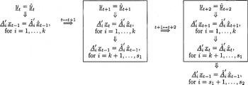
We use minimality to identify the remaining sigmoids recursively, as sketched in Figure 1. We begin with the set of indices J₁ = {k + 1,…,s₁}. Note that the definition of J₁ implies that for each i = k + 1,…,s₁ at least one of the vectors A₁,…,A_k has a nonzero ith component.

Sketch of the proof for the first three time steps. The first conclusions in the next time step t + 2 are obtained from the current time t + 1 shifted by one (framed boxes). Only the last conclusion is newly derived in each step.

We shall show that

for i = k + 1,…,s₁. Note that in the previous step we have begun at an arbitrary time t with two arbitrary

and the equation of observationally equivalence

has brought us to equation (33). In particular we have obtained

for i = 1,…,k. If we increment the time by one, we begin from

and arrive by the same reasoning at

In the last equation we can insert (34) for

with i = 1,…,k. We can use these equations to identify σ(a_k+1 + b_k+1ξ₁),…,σ(a_s1 + b_s1ξ₁) on the left-hand side with some corresponding sigmoids on the right-hand side of (37). This works because we know from the definition of J₁ that for each i = k + 1,…,s₁ there is a row vector A_j′ in (37) that has a nonzero component. In other words each σ(a_k+1 + b_k+1ξ₁),…,σ(a_k+s1 + b_k+s1ξ₁) occurs in at least one of the equations in (37). Wherever such a sigmoid occurs we can use g-IP to identify it with a corresponding sigmoid on the right-hand side of (37). As before we can then redefine

to obtain similarly to (33)

for i = k + 1,…,s₁, and

where A_i,j is the jth entry of the vector A_i. We can summarize as follows: the equation

yields

for i = 1,…,s₁ and in particular

As before the choice of t and

is arbitrary, and hence we can increment the time by one to generate from a set of equations (see also Figure 1)

the set of equations

Here we are in the same situation as in (36) except that the index i runs further to s₁. We can now consider the set J₂ = {s₁ + 1,…,s₂} and, by the definition of J₂, we can use the last equation to identify the sigmoids σ(a_s1+1 + b_s1+1ξ₁),…,σ(a_s2 + b_s2ξ₁) in x_t.

We can repeat the whole procedure until, after a finite number of steps, we arrive at (41) for all i = 1,…,n. Because

we obtain the statement of the theorem with G = S′. Formally, this part needs to be proved by induction (see also Albertini and Dai Pra, 1995). However, we think that the induction step follows evidently from Figure 1 and the preceding discussion. Apart from more indices, a formal induction would not generate further insight.

(iii) In the last part of the proof we need to relate

. Observationally equality in t = 0, i.e.,

yields

. Furthermore, we have the equation

from part (i) or (ii) (see (25) or (41) for i = 1,…,n). Inserting for

yields

. █

THEOREM 4.5. We assume that we have a strongly admissible, g-IP (with g(x) = constant/x) minimal system that is parametrized by Σ_n = (A,B,C) and a minimal system

. If

are observationally equivalent then

where

is a permutation with sign changes and Λ is a diagonal matrix with strictly positive diagonal elements.

Proof. A careful investigation of the previous proof of Theorem 4.4 reveals that all arguments remain the same except the step from equation (20) to (23). At this point the previous

turns into

and the equation

into

. The

do not change. Noting that ker(ΛA) = ker(A) we obtain the statement of the theorem. In the following discussion we shall present the steps that deviate from the proof of Theorem 4.4. All other conclusions can be copied literally from the proof of Theorem 4.4.

Similarly to part (i) in the proof of Theorem 4.4 we insert u = z₀ η + u₁ ξ, where

(u₁ and

as in Lemma 4.2(ii)). We arrive at equation (14) with

Again, by Lemma 4.2(ii) the functions

have different slopes in η, and thus we can find a nontrivial interval

in which a_i g(b_i) ≠ (±1)a_j g(b_j) for i ≠ j. As before, we can separate the functions on the left-hand side in (14), and g-IP yields

Note that the sign of (±1) (resulting from the definition of g-IP) and

are uncorrelated. First, we separate coefficients in η. Then it can be shown (exactly as in part (i) of the proof of Theorem 4.4) that j is independent of η, v, and δ. With g(x) = constant/x we obtain

which is satisfied for

for any λ > 0. Inserting this expression in (48) yields

where G is a permutation with sign changes and Λ a diagonal matrix with positive diagonal entries. From here onward the arguments are identical with the proof of Theorem 4.4. █

The last theorem and Remark 2.2 yield the following corollary.

COROLLARY 4.6. We assume that the sigmoid function in the Elman network is the Heaviside function. Furthermore, let Σ_n = (A,B,C) be a strongly admissible, minimal system and

a minimal system. Then

are observationally equivalent if and only if

where

is a permutation with sign changes and Λ is a diagonal matrix with strictly positive diagonal elements.