


1. Introduction
Countries around the world are evaluating various policy approaches to address climate change. Among these, emission reduction schemes have emerged as promising solutions. Such schemes, often taking the form of cap-and-trade systems, have been implemented in various regions, including the European Union (EU), New Zealand, California, and more recently China (Rontard and Hernandez, Reference Rontard and Hernandez2022; Doda et al. Reference Doda, Wildgrube, Ferrari and Borghesi2025). This approach establishes a maximum emission limit, or “cap,” and requires emissions exceeding this threshold to be compensated through the use of tradable permits. These permits are exchanged on secondary markets among firms. The primary markets, managed by regulatory authorities, distribute permits through auctions or free allocations. These carbon markets are mandatory: companies subject to the policy must participate, comply with regulations, or face fines for violations.
Policymakers and academics are currently discussing the potential to complement compliance carbon markets (CCMs) with a voluntary system. In this proposed arrangement, polluting companies could offset their carbon footprint by financing carbon removal activities undertaken by other entities. These are called voluntary carbon markets (VCMs) and would link companies that emit greenhouse gases (GHGs) to organizations capable of absorbing and storing them or avoiding the creation of new emissions. These carbon removal activities could be carried out by various entities, such as land managers, farmers, or firms with access to carbon-capture technologies. The technologies used might range from nature-based solutions to more intensive technological approaches. Nature-based solutions include changes in soil management, afforestation, and other land-based strategies (Paul et al. Reference Paul, Bartkowski, Dönmez, Don, Mayer, Steffens, Weigl, Wiesmeier, Wolf and Helming2023). More technologically advanced practices, such as Carbon Capture and Storage (CCS), typically involve artificial absorption of CO2 and subsequent storage in controlled stable forms (Bazzana et al. Reference Bazzana, Comincioli, Gusperti, Legrenzi, Rizzati and Vergalli2025). This market is generating around two billion USD in transactions, and some sources project it to reach 50 billion per year by 2030 (Chen et al. Reference Chen, Marbouh, Moore and Stern2021).
The primary forms of VCM include renewable energy development, the capture and storage of GHGs, and avoided deforestation. In 2020,
 $24.9\%$
of the voluntary carbon offsets (VCOs) were from the Reduction of Emissions from Deforestation and Forest Degradation (REDD+) projects,
 $17.9\%$
from wind energy, and
 $14.5\%$
from improved forest management. The EU has already evaluated the introduction of VCM along with CCM during the implementation of the Kyoto Protocol in the Clean Development Mechanism (Böhringer, Reference Böhringer2003). Under this system, companies from developed nations could generate permits by supporting afforestation or emission reduction projects in developing countries, thereby acquiring carbon offsets. However, the low costs of these activities reduced the incentive to abate or participate in CCM, driving the EU to ban offsets in the Emission Trading System (ETS) in 2012 for industrial firms (Ahonen et al. Reference Ahonen, Kessler, Michaelowa, Espelage and Hoch2022). However, the EU ETS and the United Kingdom ETS allow for offsets for the aviation sector under the Carbon offset and Reduction Scheme for International Aviation (CORSIA) mechanism. The UK is considering implementing technology-based offsets for industrial firms.Footnote
1
More recently, the European Commission has expressed renewed interest in developing effective frameworks for VCOs. The carbon market that EU institutions might have in mind should address long-standing limitations, such as credible certification processes and consistency with other environmental objectives (European Commission, 2022; Wolf, Reference Wolf2022). Countries that currently allow offset through permit trading in their carbon pricing systems are Japan, New Zealand, and, in part, California, Quebec, and China (La Hoz Theuer et al. Reference La Hoz Theuer, Hall, Eden, Krause, Haug, De Clara, Hoz Theuer and Clara2023).
VCMs have provoked skepticism among some experts, who question their stability due to potential bureaucratic inefficiencies and the dominant role of intermediaries (Milne and Mahanty, Reference Milne and Mahanty2019). Another reason is the consistency of its climate effects, which have been publicly challenged.Footnote 2 While these limitations of VCMs are relevant topics of study, they might miss deeper motivations and incentives at their core. Thus, this study offers a novel perspective by examining the stability and diffusion of VCM by endogenising market structure, making it a function of profit differentials driven by commodity, offset and permit prices, as well as abatement and compensation costs. We propose a partial equilibrium model in which VCMs operate within the same jurisdiction of CCMs, ensuring that emission reduction efforts align coherently with broader climate objectives, thereby mitigating the previous limitations. This assumption implies that the government imposes a monitoring system that removes information asymmetries and allows agents to focus on selecting quantities of offsets under optimal conditions. This assumption can be interpreted loosely in the sense that compensations might be produced in a different country that still operates with the same quality expected by the EU Commission, for example, meaning an absence of jurisdiction asymmetries (European Commission, 2024). Our model focuses on a critical, often overlooked aspect, acknowledging the complexities of permanent carbon capture and the many variations in offset technologies: the economic incentives of offset producers. This implies that we can investigate instabilities that are not directly tied to information asymmetries and other aspects mentioned above.
In the model presented hereby, firms generating offsets face incremental switching costs for each additional unit of emissions captured, proportional to the standard output of firms in their sector, which allows for a parsimonious technology taxonomy. Firms demanding offsets will incur monitoring costs. For the sake of clarity, we frame our discussion around farmers as archetypal offset producers, though the model’s implications extend to any industry engaged in offset production alongside traditional commodities.
Another key innovation of this study lies in its treatment of offset demand as a critical determinant in shaping VCM. We address the pressing issue of carbon leakage (CL), where firms might circumvent climate policies by relocating to jurisdictions with lax environmental regulations – often termed “pollution havens” (Jakob, Reference Jakob2021; Grubb et al. Reference Grubb, Jordan, Hertwich, Neuhoff, Das, Bandyopadhyay, van Asselt, Sato, Wang, Pizer and Oh2022). This phenomenon not only results in competitive disadvantages for the jurisdiction adopting carbon pricing but also undermines global climate mitigation efforts, as emissions are simply displaced rather than reduced. Our model uniquely captures how such relocations can diminish demand for carbon permits, potentially discouraging offset producers (such as farmers) from engaging in carbon-absorbing activities. This dynamic interplay between firm behavior and offset production could significantly destabilize both CCM and VCM, presenting a critical challenge to the efficacy of climate policy instruments.
To investigate these complex interactions, we employ an evolutionary model that features two groups of agents: industrial firms and farmers. Our model aims to identify equilibria in the proportions of firms participating in carbon markets on both sides of the market. The decision-making process evolves based on profit differentials, with companies entering carbon markets when profits exceed those from alternative options. For industrial firms, this alternative is relocating to pollution havens, while for farmers, it is maintaining standard business models. Equilibrium is reached when the profit differentials between the two groups shrink to zero, that is, agents have achieved a point where they are indifferent among the alternative options. The model’s dynamics are based on two replicator dynamics equations reflecting profit differentials within each group. Companies act as price-takers in four homogeneous goods markets: CCM, VCM, industrial commodities, and agricultural commodities. We analyze equilibria under three distinct scenarios. In the baseline scenario, no costs are imposed on relocating companies. The second scenario introduces a fixed relocation cost, reflecting regulatory asymmetries such as the Carbon Border Adjustment Mechanism (CBAM) or other sunk costs. The third scenario, which we term “rationing,” simulates a supply offset imposed by the administration. This final condition reflects cases of exogenous emission reduction in which offset prices adjust according to demand levels, analogously to climate-oriented agricultural policies. This comprehensive model structure allows us to examine the intricate interplay between industrial relocation, offset production, and carbon market stability under various policy conditions. The paper innovates on the existing literature by elaborating on the behavior of firms in VCM while still being subject to a CCM, which may be typical in the next phases of the European ETS. Furthermore, we adapt the models of dual production for emission absorption in a setting of bounded rationality, diverging from the cases of social planner problems in offsets.
The findings reveal that, without intervention, VCM demand collapses as firms relocate. Introducing relocation costs significantly alters this dynamic, possibly eliminating CL and increasing VCM participation, especially with the addition of offset technologies. Offset rationing can maintain higher VCM shares even with substitute technologies. The study highlights the contingency of policy effectiveness in emerging VCM practices. It concludes that both relocation costs and offset rationing policies substantially enhance overall welfare levels, providing valuable information for the design of climate policy. The work is structured as follows. The literature review (Section 2) presents the scientific background behind our methodology and claims. The model’s establishments will then describe how agents behave in these markets in Section 3 containing profit functions, market-clearing conditions, and the evolutionary dynamics. The equilibrium analysis is delivered afterward in Section 4, where calibration, welfare, and sensitivity analyses are provided: evidence of parameters anchoring in the literature and robustness is addressed. Section 5 discusses the policy implications of VCO implementation alongside CCM and their relation to carbon dividends, a relevant element of climate taxation. A specific subsection elaborates on the limitations of this study. Section 6 concludes with the innovative aspects provided by our work.
2. Literature
The model is rooted in the literature on CL dynamic models, borrowing various elements. Relocation of companies represents a significant policy issue that has prompted several streams of research. This follows from the loss of competitiveness of local firms against international ones, which may operate under less environmentally stringent conditions. Relocating firms to such jurisdictions may increase pollution, thereby undermining the environmental benefits of emission reductions within the CCM’s jurisdiction. Offshoring industrial activities not only affects the environment, but also affects local economies by reducing labor bargaining power and displacing workers (Radi et al. Reference Radi, Lamantia and Italo Bischi2021).
Given its relevance to policy, various conceptualizations have emerged to assess CL drivers and potential balancing mechanisms. Böhringer et al. (Reference Böhringer, Carbone and Rutherford2012) evaluated three possible solutions to CL: border tax adjustments, regulatory exemptions, and output-based allowance allocation. They concluded that no solution fully resolves the trade-off between efficiency and equity between countries. Although border tax adjustments are shown to be most effective in reducing CL, they can exacerbate regional inequality. Monjon and Quirion (Reference Monjon and Quirion2011) assessed different border adjustment configurations using a partial equilibrium model. Their findings suggest that a CBAM policy could limit leakage and decrease the production of emission-intensive products. Böhringer et al. (Reference Böhringer, Rosendahl and Storrøsten2017) demonstrated that combining output-based rebating with a consumption tax on goods containing emission and exposed to trade can be equivalent to a border carbon adjustment, potentially improving the welfare of regions implementing emission pricing. Analyzing the allocation rules for auctioning exemptions in the 2009 ETS Directive, Clò (Reference Clò2010) argued that these rules are politically driven. The author contended that grandfathering is unlikely to mitigate CL effectively, instead potentially increasing competition distortions and hampering harmonization within the Emissions Trading System (ETS).
Provided the theoretical basis for CL and its countermeasures, empirical studies have attempted to assess the actual impacts of climate policies on competitiveness. Assogbavi and Dées (Reference Assogbavi and Dées2023) studied whether an increase in the stringency of environmental policies affected CL. They do so with a gravity model on a panel dataset and find no evidence of CL through international trade at the global level. However, they find evidence of leakage for importing countries with more stringent policies. Grubb et al. (Reference Grubb, Jordan, Hertwich, Neuhoff, Das, Bandyopadhyay, van Asselt, Sato, Wang, Pizer and Oh2022) reviewed the state-of-the-art trade in energy-intensive goods and found that aggregate emissions transfers from developing to developed countries peaked in 2006 and have since declined. This is also a consequence of shielding the most emission-intensive sectors from governments. Jakob (Reference Jakob2021) highlights how more stringent climate policies that need to meet targets might trigger CL. Simulations with numerically computable general equilibrium models provide an average figure of
 $14\%$
for the future CL. The review by Verde (Reference Verde2020) finds that climate policies yielded statistically insignificant effects of ETS on the competitiveness of regulated or CL. However, this is tested on the first two phases of the ETS alone, when prices were comparatively low compared to 2022 and 2023. The demand for allowances was furthermore depressed by a negative business cycle and a relaxed policy of free allowances. The overcompensation was determined by the allocation to firms exposed to CL, which reduced the general efficiency of the system (Martin et al. Reference Martin, Muûls, de Preux and Wagner2014b). It took years for CCM prices to reach a sufficient level and drive abatement after the activity of the Market Stability Reserve and the stricter Cap provision under the Fit-for-55 package (European Commission, 2020).
Regarding the modeling approach, we consider foundational to our work the studies on the behavior of firms in CCM in the presence of free allowances. Antoci et al. (Reference Antoci, Borghesi, Iannucci and Sodini2021) study the possible delocalization consequences of ETS through an evolutionary model. The ETS price, free allowances, and the emission cap level influence the decision to relocate. Their simulations show that the relocation decision is more sensitive to cost-reducing policies related to green technologies. Antoci et al. (Reference Antoci, Borghesi and Russu2022) consider three possible strategies for firms: going green, emitting while purchasing allowances, and relocating. Simulation reveals cyclical behavior and potential extinction of leakage under specific parameter configurations. For instance, reducing or phasing out free allowances can cause firms to stop producing dirty products, and vice versa. Tampieri and Iannucci (Reference Tampieri and Iannucci2023) develop an oligopoly of profit-seeking and environmentally socially responsible firms and study the effects of an environmental tax and an abatement technology. They find that a policy mix of tax and subsidy maximizes the environmental benefits. Following their conclusions and improving on Antoci et al. (Reference Antoci, Borghesi, Iannucci and Sodini2021), we introduced VCM in the policy mix to assess the implications of CL. Instead of adopting a proportional tax, as in previous research (Böhringer et al. Reference Böhringer, Carbone and Rutherford2012; Antimiani et al. Reference Antimiani, Costantini, Martini, Salvatici and Tommasino2013), we investigated a regulation imposing a fixed cost on relocating firms, which proxies asymmetries in the regulatory frameworks of jurisdictions. A real case of such an asymmetry is represented by the due diligence costs associated with monitoring emissions and environmental liability, which are exogenous to the importer’s dimension and can be cumbersome for trade relations.
For simplicity, our model considers VCM supplied by nature-based solutions involving farmers or land managers. We introduce a switching cost in the farmer’s profit function to capture the substitutability between emission-absorbing activities and traditional farming methods. The switching cost parameter, which we will describe in detail in the model section, should quantitatively capture the effort a company must undertake to adopt substitute practices. Thus, generating offsets is tied to substitutions of previous activities. We provide a synthetic review of various technologies in nature-based solutions for generating offsets in Table 1. We define “substitute” any activity or a technology that impedes farmers from operating mainstream business activities on the same land. In other cases, VCM will require land managers to implement additional practices in conjunction with their current ones. If a practice or technology presents no switching costs, it can be considered “additional.”
Examples of different offset activities and mapping to this article taxonomy

Table 1. Long description
A table comparing various offset activities and their characteristics. The table has six rows and six columns. The columns are labeled Examples, Description, Technology, Type, This paper’s Class, and Reference. The rows are as follows: Row 1: Examples, Agroforestry; Description, Forest farming for uses different from biogas; Technology, Natural; Type, Removal; This paper’s Class, Substitute; Reference, (Sharma et al. 2021; Nyssen, 2021). Row 2: Examples, Avoided Deforestation or Emissions; Description, Proof that without carbon farming, a natural carbon sink would have been removed; Technology, Natural; Type, Avoidance; This paper’s Class, Substitute; Reference, (Lee et al. 2018; Groom and Venmans, 2023). Row 3: Examples, Adoption of Green practices; Description, Efficient energy systems, Gross reduction in emissions proving evident reduction compared to BAU; Technology, Technological; Type, Reduction; This paper’s Class, Additional; Reference, (Karhunmaa, 2016). Row 4: Examples, Soil Management; Description, Using agriculture to absorb CO2e, by adopting sustainable land management; Technology, Technological; Type, Removal; This paper’s Class, Additional; Reference, (Nyssen, 2021; Paul et al. 2023). Row 5: Examples, Bioenergy with Carbon Capture and Storage (BECCS); Description, Excess biomass is burnt for energy, emissions are artificially stored; Technology, Technological; Type, Removal; This paper’s Class, Additional; Reference, (Zetterberg et al. 2021; Tamme and Beck, 2021).
This classification encompasses existing channels for offset of CO2e emissions (Roman-Cuesta and Borghesi, Reference Roman-Cuesta and Borghesi2022). In particular, the most relevant and legally supported method is the removal of GHG, which can be done through natural (forestry) or artificial means. Moreover, substitute practices may also involve emissions avoidance, such as preserving forests on agricultural land. Additional practices help reduce emissions following the adoption of green strategies and technologies.
3. Model
The model comprises two interacting agent groups, each operating in two markets, one of which is shared: the VCM. The groups consist of a fixed number of firms, divided into two subgroups. Firms within each subgroup are homogeneous in terms of production functions and demand for offsets and allowances. All commodities in the model are homogeneous. Industrial companies can reduce emissions linearly through abatement or offsets. However, they must compensate for their emissions by purchasing allowances on the CCM. The industrial group consists of
 $N$
firms, of which
 $xN$
have relocated outside climate regulation jurisdictions, while
 $(1-x)N$
remain within regulated areas. Industrial firms produce commodities and can decide whether to participate in carbon markets. The farmer group comprises
 $N_a$
companies,
 $yN_a$
producing compensatory products along with agricultural products that are distinct from the industrial commodity, and
 $(1-y)N_a$
maintaining traditional business models. The dynamic variables of the model are the CL share,
 $x$
, and the offset farmers’ share,
 $y$
, with
 $N$
and
 $N_a$
remaining constant.Footnote
3
3.1 Manufacturing firms
The home firms
 $h$
comply with the climate policies and have a profit function
 $\Pi ^{h}$
as presented in Equation (1).
 \begin{equation} \Pi ^{h}=pq_h-\frac {1}{2}q^{2}_h\underbrace {-\frac {\theta }{2}z^{2}-a\,(q_h-z-c)}_{\textrm {CCM}}\underbrace {-\frac {\eta }{2}c^{2}-b\, (c)}_{\textrm {VCM}} \end{equation}
Gross revenues are the product of prices
 $p$
and quantities
 $q_h$
. The costs, which have a quadratic structure, originate from production, abatement, and offset. They include the amount of permits and offsets purchased,
 $z$
and
 $c$
, respectively, as well as their CCM and VCM prices,
 $a$
and
 $b$
. We adopt a quadratic cost function to achieve linear marginal costs in production, abatement, and offset use. Considering offsets to be nonlinear could be attributed to search costs, information asymmetries, and intermediary fees (Drechsler, Reference Drechsler2022). Intermediaries are excluded; therefore, industries incur the costs of Measuring, Reporting, and Verifying (MRV) offsets to comply with quality standards. The quadratic form synthesizes this dynamic well, being previously used in addressing competition among groups of firms, even in the case of offsets (Jones and Mendelson, Reference Jones and Mendelson2011; Wang and Wang, Reference Wang and Wang2015).
 $\theta , \eta$
are the efficiency of the abatement and offset processes. Fixed costs are null in home firms.
The profit function of relocating firms
 $r$
presents a form such as in Equation (2).
 \begin{equation} \Pi ^{r}=pq_r-\frac {1}{2}q^{2}_r - R \end{equation}
Companies relocating avoid climate policy costs, while facing a fixed cost
 $R$
. This feature could be intended as an implicit sunk cost of investing in a foreign market, as well as the bureaucratic burden of dealing with border authorities. Except for the fixed cost structure, the relocating firms present identical marginal costs to the home industry. However, these companies do not need to interact with the regulators to buy permits or with land managers for offsets.
3.2 Offset and agricultural firms
We characterize the land sector participating in offset as comprising small, homogenous companies with no ability to unilaterally influence agricultural market equilibrium. As in European agriculture, where farmers typically own less than five acres and operate family businesses (Cook, Reference Cook2020). These farmers or land managers operate under carbon-neutral premises, or under a regulation that exempts their activities in some fashion from the same monitoring rules as those of industrial firms. They can make their activities carbon-negative to produce an offset, or at least reduce their emissions from the benchmark if we consider looser regulatory standards. For simplicity, we will ignore the distinction between removal and reduction. The agricultural market considered in our model is assumed to be independent of the dynamics of companies involved in climate policies. Consequently, we have incorporated this independence implicitly into the model’s evolutionary dynamics.
The management of land for offset purposes necessitates the introduction of new practices to integrate them into mainstream activities. As the literature review highlights, these can take two main forms: substitute offsets (CO) or additional offsets (AOs), translating into different degrees of substitutability with standard practices. The profit function of the offset agricultural firms is the following Equation (3).
 \begin{equation} \Pi ^{o}= p_a q_o - \frac {c_a}{2}q^2_o + b s-\frac {c_o}{2}s^2 -\psi s q_o \end{equation}
With
 $q_o$
being the quantity of agricultural goods produced by offset firms, and
 $s$
the quantity of offsets.
 $\psi$
represents the switching cost between the two activities and is partially influenced by the literature on divisionalized firms (Hirshleifer, Reference Hirshleifer1957). When the value of the switching cost parameter is zero, the marginal cost of offsets is unrelated to agricultural products and vice versa. On the contrary, whenever it is positive, the marginal cost of offsets increases proportionally to the quantity of agricultural products. The increased cost is proportional to
 $\psi$
, meaning that the greater the parameter is, the more relevant the substitution cost, hence the stricter the substitutability.
If the market price of the offset is null, land managers in offsets can still use agricultural products and maintain climate-relevant production at zero, thereby avoiding switching costs. The simplification we considered here is the price homogeneity between traditional agriculture and the commercial element, offset by the value of byproducts. The offset agricultural firms of both types compete with the traditional business model. The companies within the latter approach do not present any share of land for absorbing GHG and, therefore, rely solely on the revenues of standard agricultural activities, driven by the price
 $p_a$
, as shown in Equation (4).
 \begin{equation} \Pi ^{a}=p_a q_a - \frac {c_a}{2}q^2_a \end{equation}
The profit structure from traditional agricultural activities remains unchanged in the evolutionary process. In this sense, they serve as a benchmark against which the offset activity is compared.
3.3 Market-clearing conditions
The model presents four markets, whose clearing conditions are defined simultaneously. The distributions of agents within each subgroup determine the prices by presenting their optimal supply to the market. Industrial companies also have an optimal demand in the offset market. The supply of CCM is determined exogenously by the regulator.
Commodities market: The first market presented here is where the population of
 $N$
industrial firms sell their commodities. As a first attempt at modeling the interaction of VCO and CL, we focus on a scenario of perfect competition, where price-taking companies of a homogeneous commodity sell optimal quantities of products. The market-clearing condition is presented here as an inverse demand function:
 \begin{equation} p=\hat {p}-(1-x)Nq^{*}_h-xNq^{*}_r. \end{equation}
We consider an elastic demand, where
 $\hat {p}$
is the reserve price. The market price
 $p$
follows after the firms set the optimal quantities
 $q^{*}_h, q^{*}_r$
, representing production in either the home or relocation market, with
 $x$
being the latter’s share.
Emission permits market: The production of industrial commodities generates emissions. Companies operating within the jurisdiction are required to participate in compliance markets and limit their emissions according to a limit known as the cap. This sets the second market-clearing condition:
 \begin{equation} (1-x)N(q^{*}_h-z^{*}-c^{*})=Q \end{equation}
The equilibrium in the allowance market is found where the fixed supply of permits
 $Q$
meets the demand from home industrial firms, the proportion
 $(1-x)$
. According to its climate objectives, the administration sets the cap on allowances at the start of the regulatory process. The demand is then formulated according to an optimal production decision. This quantity equals the emissions minus abatement
 $z^{*}$
and the offset quantity
 $c^{*}$
. VCM emerge then as buffers and, in theory, should reduce the risk of price spikes.
Offsets market: The third market-clearing condition is where offsets supply meets demand. The former corresponds to the land devoted to GHG absorption. The latter refers to the number of offsets purchased by the domestic firms subject to CCM:
 \begin{equation} (1-x)N(c^{*})=yN_a s^* \end{equation}
Thus, the left-hand side of this equation is the demand for offsets, and the right-hand side is the supply, which is equal to the product of the number of offsetters
 $yN_a$
and the optimal production of offsets
 $s^*$
. The equilibrium is therefore endogenous to the structure of both the agricultural and industrial sectors.
Agricultural market: The agricultural market similarly allocates commodities to the industrial market. An inverse demand function ties the agricultural prices to a reserve price
 $\hat {p}$
reduced by the quantities produced optimally.
 \begin{equation} p_a=\hat {p}_a-(1-y)Nq^{*}_a-yNq^{*}_o. \end{equation}
The demand for agricultural products is elastic in this case. Mainstream and offsetters are price-takers in this market as well. The three equations are solved in a system at each iteration and are then plugged into the firms’ profit structure. The shares
 $x$
and
 $y$
at time
 $t+1$
are generated using an evolutionary algorithm.
3.4 Evolutionary dynamics
The VCM and CCM markets interact through two similar replicating dynamics algorithms, à la random matching game proposed by Weibull (Reference Weibull1997). These dynamic functions calculate the portion of companies relocating at every iteration based on where more profit is generated. For example, the costs of climate policies drive the share of firms involved in carbon markets. If there are greater profits in relocating, CL will increase. The VCM diffusion is endogenous to the equilibrium between the demand side of home industrial firms and the supply side of land managers involved in offset activities. Companies transition from a traditional agricultural business model to a carbon-negative production approach only if there is a financial benefit to doing so. The markets are in equilibrium if there is indifference in the selection of the business model and the location, thus stability is found in the population shares
 $x$
and
 $y$
. The agents select their production strategies based on efficiency, but they acquire this information “slowly.”
The number of
 $N$
industrial firms decides whether to stay home or relocate their activities by comparing the profit differences and considering the opposing side. If staying within the jurisdiction of the climate law, the population of companies
 $(1-x)N$
can buy allowances or offsets. In contrast, if profits from relocation are greater, a proportion of firms will relocate. The differences in profits determine the proportion of firms relocating. The replicating algorithm is therefore equal to:
 \begin{equation} \dot {x}_t = x_t(1-x_t)\Delta _t \Pi ^f(x_t,y_t) \end{equation}
The profit differential of industrial firms
 $f$
is
 $\Delta _t \Pi ^{f}= \Pi ^{r}-\Pi ^{h}$
, and when it is equal to zero, the share reaches equilibrium. The group of relocating firms indirectly influences the VCM. Participation in such trade is voluntary for both agricultural and industrial firms. Allowances are sold through auctions regulated by an external authority, influencing directly the former replicating algorithm, and are fixed. The proportion of agricultural firms participating in offset production, denoted by
 $y$
, evolves according to the profit differentials following replicator dynamics. This value determines the supply of offsets.
 \begin{equation} \dot {y}_t = y_t (1-y_t) \Delta _t \Pi ^l(x_t,y_t) \end{equation}
The share of agricultural firms involved in offset stabilizes as
 $\Delta _t \Pi ^{l}=\Pi ^o-\Pi ^a=0$
. In synthesis, the agents will use the information available in the price signals at time
 $t$
to identify the production strategies which affect the profit dynamics, which in turn determine the evolutionary shares
 $x$
and
 $y$
for time
 $t+1$
. The markets adjust from the economic performances of
 $q^*_h$
,
 $z^*$
and
 $c^*$
at time
 $t$
and produce new signals for
 $t+1$
. They will adjust the supply and demand after receiving information about changes in the market structure.
Thus, the VCM is the meeting of two evolutionary processes. One resides on the demand side, with industrial firms not relocating and interested in offsetting their activities. The supply is characterized by the agricultural firms willing to participate in VCM. The equilibrium of offset practices in the agricultural sector is found when the two evolutionary processes reach stability.
Some insights into the equilibrium in carbon markets can be gained by solving each profit differential separately. The industrial firms will decide whether to move according to the cost of participating in CCM net to VCM, as shown in Equation (11).
 \begin{equation} \Delta _t \Pi ^f= \frac {1}{2}a^2+a(p-a)-\frac {1}{2}\frac {a^2}{\theta }-\frac {1}{2}\frac {(a-b)^2}{\eta }-R \end{equation}
The costs of abatement
 $\frac {1}{2}\frac {a^2}{\theta }=z^*$
and offset
 $\frac {1}{2}\frac {(a-b)^2}{\eta }=c^*$
must be greater than the cost of demanding CCM permits
 $a(p-a)=aq^*_h$
and a wedge in operation’s profitability for firms to remain in the jurisdiction of climate regulation. The relocating cost
 $R$
generates a burden that further deters firms from abandoning climate mitigation efforts. This profitability wedge is
 $\frac {1}{2}a^2-R$
. Optimal production in home firms includes carbon price, thus, barrier
 $R$
reduces the profitability wedge, while CCM price
 $a$
augments it according to the cost structure. The achievement of this condition is based on the value of the cost of relocating. In case
 $R\gt \frac {1}{2}a^2$
, all industrial firms will eventually participate in CCM and VCM. The alternative channel for increasing the competitiveness of local firms is a reduction in the offset price, since
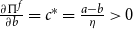 $\frac {\partial \Pi ^f}{\partial b}=c^*=\frac {a-b}{\eta }\gt 0$
. Such a reduction would diminish the alternative channel of emission reduction and also mitigate the demand on CCM, depressing permit prices. Policy mechanisms intended to boost the supply of offsets could have this effect. A similar reasoning can be established for the diffusion of offsetters in the agricultural sector, driven by the differences in profit from Equation (12).
 \begin{equation} \Delta _t \Pi ^l =-\frac {1}{2}\frac {(b-\psi p_a)^2}{(\psi -1)(1+\psi )} \end{equation}
If the differentials in agricultural profits are negative, it means that the share of carbon-negative land managers capable of supplying offsets will decrease over time. For simplicity, we will assume that the factors of marginal costs were similar across agricultural practices (
 $c_a=c_o$
), meaning that mainstream farmers and offsets activities have similar marginal costs. Since offsets must be produced by firms that have already achieved net neutrality, it is fair to assume that offset activities have similar marginal cost factors associated with carbon-neutral farm products. In this case, if the switching cost is not sufficiently low (
 $\psi \lt 1$
), there is no marginal profit wedge that can explain the diffusion of offsets without some exogenous policy driver. Conversely, the greater the distance between the marginal revenues of offsets and agricultural prices (adjusted for switching practices), the greater is the share of land managers involved in VCM. Therefore, we should expect substitute practices to be less competitive than additional ones in a system that involves perfect information and linear marginal costs of offsets and monitoring without policy intervention.
3.5 model’s solution and scenarios under different policies
The literature has presented several common elements in addressing CL. Policy mixes, for instance, tend to enhance abatement effectiveness and bolster the competitiveness of local businesses. However, the role of offsets as auxiliary policies has not yet been thoroughly examined. Notably, the relationship between offset activities and CL remains unclear, in contrast to the extensively investigated effects of free allowances. The CBAM represents another proposed policy aimed at mitigating CL. Consequently, equilibrium results for a model incorporating both CL and VCO should consider these varied policy settings.
We will then consider the role of VCO in three different scenarios: under no constraint, under a carbon tariff, and with the possibility of rationing the demand for offsets. This is because the involvement of VCM in the compliance market presents potential risk factors for the institutions and other stakeholders. We investigate the possibility of the administration limiting the use of offsets and adopting a tariff to deter firms from relocating. It is worth noting that these different settings impact the structure and closure of the baseline model presented in the previous subsections. In particular, the optimal quantities vary according to the policy in place. Therefore, in this subsection, we elucidate these differences.
3.5.1 Free entry–exit
We elaborate first on the case of the market as a reference, where the administration does not intervene to stop the demand for offsets or limit CL. The industry sector at the international level is composed of price-takers with no exogenous constraints. Thus, home firms produce an optimal quantity
 $q_h^{*}=p-a$
, abating always an amount
 $z^{*}=\frac {a}{\theta }$
, proportional to the price of abatement. The offset used equals
 $c^{*}=\frac {a-b}{\eta }$
, always proportional to the price gap between the compliance and voluntary markets. Finally, the relocating firms produce an optimal quantity
 $q_r^{*}=p$
.
3.5.2 Relocation fixed cost
In this scenario, the relocating firms face a constant and strictly positive cost
 $R\gt 0$
. Since
 $R$
enters only the level of profits and not the marginal conditions, optimal quantities and marginal profits are identical to the free entry–exit case, while total profits of relocating firms are reduced. This policy aims to keep companies operating in the climate jurisdiction by narrowing the profit differential
 $\Delta \Pi ^f$
.
The parameter
 $R$
is best interpreted as a reduced-form proxy for the net present value of the costs associated with relocation – including due diligence, regulatory compliance, and the sunk cost of establishing operations in a foreign jurisdiction – rather than a per-period fee. In the replicator dynamics framework, where agents compare flow payoffs and adjust population shares gradually,
 $R$
captures the amortized burden of relocation that depresses the profitability of the relocating strategy at each pairwise comparison. Relevant asymmetries in regulation for imported commodities could generate such effects. For instance, the CBAM requires reporting emissions according to technical standards since its early phases. The effort to abide by this regulation constitutes a sunk cost for firms that intend to relocate abroad.Footnote
4
3.5.3 Exogenous rationing
The last policy we implemented is standardizing offset activities for the firm. The Chinese ETS is an example of such experimentation, where 5% of surrendered permits can be generated using VCM (La Hoz Theuer et al. Reference La Hoz Theuer, Hall, Eden, Krause, Haug, De Clara, Hoz Theuer and Clara2023). For simplicity, we presumed that the amount of offsets should have been proportional to the cap of the nation and adjusted to the number of companies that have not relocated, such that:
 \begin{equation} \hat {s}=\frac {Qf}{N_a} \end{equation}
The coefficient
 $0\lt f\lt 1$
indicates the amount of emissions that offsetters will compensate and is decided by the regulator. In the end, the emissions within the climate jurisdiction will always equal
 $Q(1+f)$
, where
 $Q$
represents the regulated amount and
 $Qf$
represents the offsetters. Under this rule, the quantity of agricultural goods produced changes to
 $q_o^*=\frac {p_a-\hat {s}\psi }{c_a}$
, being the supply exogenous to the firm behavior.
4. Equilibrium analysis
The model involves two interacting differential equations constructed around two fixed populations of agents. Changes are driven by differences in profits, which are assumed to be exogenous to the market-clearing conditions. At this point, we can state that differential Equations (9 ) and (10) are functions of shares
 $x$
and
 $y$
. The stability of each equilibrium point is assessed by calculating the trace and determinant of the Jacobian Matrix generated from the system of differential equations.
 \begin{equation*} J(x,y)=\begin{Bmatrix} \dfrac {\partial \dot {x}}{\partial x} & \dfrac {\partial \dot {x}}{\partial y} \\[10pt] \dfrac {\partial \dot {y}}{\partial x} & \dfrac {\partial \dot {y}}{\partial y} \end{Bmatrix} \end{equation*}
The steady states are found when the variables do not change, as Equations (12) and (13) indicate. Departing from a system of equations comprising Equations (9) and (10), the steady states are calculated by imposing the
 $\dot {x}$
and
 $\dot {y}$
to equate zero and solving for
 $x$
and
 $y$
. This approach has been repeated for each policy case, producing various equilibrium points in each one, which are added to (0,1), (1,1), (1,0), and (0,0). This diversity of equilibrium derives from the nonlinearities in the system of differential equations. The impossibility of achieving a generalized solution requires us to calibrate the system of equations following previous literature and impose assumptions on our study. Furthermore, the calibration enables a more intuitive interpretation of the welfare that consumers obtain at each equilibrium point.
4.1 Calibration
The calibration parameters for our baseline explorative solution are presented in Table 2.
The set of parameters for model calibration

Table 2. Long description
A table titled ‘The set of parameters for model calibration’ with six columns and eleven rows. The columns are labeled ‘Parameter’, ‘Description’, ‘Value’, and ‘Source’. The table lists various parameters used for model calibration, their descriptions, corresponding values, and sources. Row 1: Parameter, Did, 9; Description, Number of firms, N; Value, 50; Source, Antoci et al. (2019). Row 2: Parameter, T; Description, Periods; Value, 100; Source, Authors selection (see Section 4.1). Row 3: Parameter, N a; Description, Number of agricultural firms; Value, 30; Source, Authors selection (see Section 4.1). Row 4: Parameter, Q; Description, Amount of permits (CAP); Value, 50; Source, Authors selection (see Section 4.1). Row 5: Parameter, f; Description, Exogenous offset for each firm; Value, 0.2; Source, Authors selection (see Section 4.1). Row 6: Parameter, c b; Description, Variable Cost Factor for Offset; Value, 1; Source, Authors selection (see Section 4.1). Row 7: Parameter, c a; Description, Variable Cost Factor for Main product; Value, 1; Source, Authors selection (see Section 4.1). Row 8: Parameter, ψ; Description, Switching cost; Value, 3 or 0; Source, Authors selection (sensitivity analysis in Section 4.4). Row 9: Parameter, p with hat; Description, Reserve price for industrial goods; Value, 150; Source, Antoci et al. (2019). Row 10: Parameter, p a with hat; Description, Reserve price for agricultural goods; Value, 25; Source, Authors selection (see Section 4.1). Row 11: Parameter, η; Description, Efficiency in abatement; Value, 1; Source, Authors selection (see Section 4.1). Row 12: Parameter, n; Description, Efficiency in offset; Value, 1; Source, Authors selection (see Section 4.1). Row 13: Parameter, x 0; Description, Initial value for relocating firms share; Value, 0.01; Source, Authors selection (see Section 4.1). Row 14: Parameter, y 0; Description, Initial value for offset agricultural firms share; Value, 0.2; Source, Authors selection (see Section 4.1). Row 15: Parameter, R; Description, Fixed cost for relocating activities; Value, 5; Source, Authors selection (sensitivity analysis in Section 4.4).
To justify the parameter selection, we calibrated the evolutionary models consistently with Antoci et al. (Reference Antoci, Borghesi, Iannucci and Sodini2021, Reference Antoci, Borghesi, Iannucci and Russu2019) where possible. We set the remaining parameters based on three specific assumptions listed below.
-
1.
 $c_o=c_a$
-
2.
$0\lt \frac {\hat {p}_a}{N_a} \lt 1$
&
$\frac {\hat {p}}{N} \gt 1$
-
3. No fixed costs of production


The first was indicated in Section 3.4, meaning that the generation of offsets costs as much as any other agricultural product in a carbon-neutral (or carbon-exempt) agricultural sector. Secondly, we presumed that the agricultural production is well developed compared to the offset activities. The second point relates to the dimensions of consumers’ reserve prices. Developed countries tend to dedicate relatively smaller shares of their income to agricultural products, while a greater proportion is allocated to commodities such as electronics, clothing, and vehicles. For this reason, we considered the relative market dimension for agricultural commodities to be less than unity. Conversely, industrial commodities had a relative market dimension greater than unity. Finally, in the third point, we omitted fixed production costs in all production systems for simplicity, unless imposed by an external policy.
For some parameters where values might particularly impact the dynamics, such as relocation or switching costs,
 $R$
and
 $\psi$
, we set a first tentative value and subsequently perform a sensitivity analysis in Section 4.4. The initial values for population shares
 $x$
and
 $y$
reflect realistic starting conditions with a majority of domestic and agricultural firms, while maintaining small nonzero fractions to enable replicator dynamics when economic conditions favor strategic switching.
Regarding the timeframe, we set
 $T$
such that each simulation tick should not be interpreted as a year, but rather as an abstract iteration period necessary to verify the stability of the results. Considering realistic timeframes for CCMs, we could potentially link each tick to a unit shorter than a year, such as a trimester. However, differences may exist in how different markets settle.Footnote
5
The results are presented by type of offset practice considered. Furthermore, the role of policies is addressed specifically in each case.
Free Entry–Exit scenario phase diagram for the evolution of the share of relocating firms (
 $x$
) and offset firms (
 $y$
). Sample trajectories in red, equilibria as red dots. Panel (a): Additional offsets (
 $\psi =0$
). Panel (b): Substitute offsets (
 $\psi \gt 0$
).

4.2 Results
We denote an equilibrium as
 $[x,y]$
. The free entry–exit scenario is illustrated by the phase diagrams in Figure 1(a) and (b), with sample trajectories highlighted in red. We begin with the substitute case (Figure 1(b)), which exhibits simpler dynamics. Here, we observe multiple equilibrium points:
 $[0,1]$
is a source (indicating instability and repulsion of trajectories),
 $[0,0]$
is a saddle point,
 $[0.77,1]$
is an unstable node reachable only when
 $y=1$
, and
 $[0.66,0]$
is a stable node. The absence of costs for avoiding climate policies drives companies out of the CCM jurisdiction, leading farmers to exit the VCM as demand for offsets diminishes. The system settles at an equilibrium with high levels of CL (
 $x \approx 0.66$
) and no offset supply (
 $y = 0$
). The additional case (Figure 1(a)) presents more complex dynamics, featuring a string of stable points along the
 $x=0.66$
line. The main insight is that additionality allows offset firms to persist even in the absence of policy and CL. However, this outcome is highly dependent on initial population conditions. For realistic initial values of
 $y$
(
 $y \lt 0.1$
), the stable equilibrium point would be
 $[0.66,0]$
, mirroring the substitute case.
The second case (relocation fixed cost) reflects the presence of asymmetries in regulatory systems expressed as a positive relocation fixed cost of
 $R$
. The level of substitutability affects the number of equilibria available and the location. Figure 2(a) presents the case of
 $\psi =0$
, where
 $[0,0]$
is a source. The stable node is
 $[0,1]$
, meaning that all that farmers could do is simply “add” carbon removal activities. The demand for offsets is maximum, as the relocation cost deters CL and keeps companies within the jurisdiction. The equilibriums are split into four ones if substitutability is added. The stable node becomes a source, while
 $[0,0]$
and
 $[0.1,1]$
are saddle points. In this case, the stable node is
 $[0.064,0]$
. Substitutability makes offset less competitive than ordinary permits, making the VCM collapse even in the case of a very low level of CL.
Relocation fixed costs scenario phase diagram for the evolution of the share of relocating firms (
 $x$
) and offset firms (
 $y$
). Sample trajectories in red, equilibria as red dots. Panel (a): Additional offsets (
 $\psi =0$
). Panel (b): Substitute offsets (
 $\psi \gt 0$
).

Finally, the case of rationing is discussed. If switching costs are null, such that offsets are additional, there are only two equilibrium points. Figure 3(a) indicates that
 $[0,0]$
is an unstable saddle point, for which the initial point would necessarily be
 $y=0$
. However, the stable node is
 $[0,1]$
as for the previous case. This implies that rationing does not reduce the number of offsetters if carbon removal activities are additional to the ordinary ones.
Exogenous rationing of offsets scenario phase diagram for the evolution of the share of relocating firms (
 $x$
) and offset firms (
 $y$
). Sample trajectories in red, equilibria as red dots. Panel (a): Additional offsets (
 $\psi =0$
). Panel (b): Substitute offsets (
 $\psi \gt 0$
).

The rationing guarantees a stable level of farmers in VCM, even with switching costs. Furthermore, the CBAM deterred companies from relocating. The case of substitutability, as portrayed in Figure 3(b), presents one saddle point in
 $[0,1]$
and one stable point in
 $[0,0.17]$
. Substitutability makes offsets less competitive than ordinary permits, causing the VCM to collapse even with very low levels of CL.
4.3 Welfare analysis
It is interesting at this point to evaluate the desirability of each scenario besides just the shares of
 $x$
and
 $y$
. The welfare analysis in this paper follows the standard approach of aggregating the consumer surplus, considering economic and environmental costs. Since there are two main consumer commodities, there are two surpluses to consider in the partial equilibrium analysis. One is the industrial sector, while the other relates to the agricultural sector. Thus, the total welfare is calculated as the sum of the two welfare functions as in
 $\mathcal{W}=W_i+W_a$
. In both subcases, the social planner does not optimize the welfare function; rather, the outcomes emerge from the evolutionary dynamics and can be compared post hoc. The surplus in industrial commodities accounts for the economic cost of production within the jurisdiction of the climate policy. Relocated firms outsource their production, shifting costs to other locations while continuing to sell commodities in the domestic economy. Environmental costs are equated to pollution, which we simplify by assuming an emission intensity of unity, calculated as production minus abatement and offset. Consequently, abatement or emission compensation activities directly enhance welfare. Products from relocated activities are cheaper but incur the welfare cost of unabated emissions.
Specifically, the term
 $(q_h^*-z^*-c^*)$
in Equation (14) captures residual emissions per home firm: each unit of production generates one unit of environmental damage unless neutralized by abatement
 $z$
or offsetting
 $c$
. Relocated firms, by contrast, generate damages equal to their full output
 $q_r^*$
, since they operate outside the climate jurisdiction and neither abate nor purchase offsets; the factor
 $p-1$
in the second term reflects the net surplus from their cheaper production, discounted by the unit environmental cost.
 \begin{equation} W_i = N(1-\hat {x}) \left [p q_h^* - \underbrace { \left (\frac {1}{2}(q_h^*)^{2} + \frac {1}{2}z^* + \frac {1}{2}c^* \right )}_{Economic Costs} - \underbrace {(q_h^* - z^* - c^*)}_{Damages} \right ]+N\hat {x}\left [(p -1)q^*_r \right ] \end{equation}
The welfare function aggregates the net consumer surplus from agricultural products and considers the products relevant for the consumers. However, the cost of producing offset is also in agricultural products. Thus, we added the economic costs of offset activities in the welfare analysis.
 \begin{equation} W_a = N_a \hat {y} \left [ p_a q^*_o+bs - \left ( \frac {c_a}{2}(q^*_o)^2 +\frac {c_o}{2}(s^*)^2 +\psi s^* q^*_o \right ) \right ] + N_a(1-\hat {y}) \left [p_a q^*_a - \frac {c_a}{2}(q^*_a)^2 \right ] \end{equation}
Since we assumed that the sector was producing offsets that were already net-neutral to the climate, we assumed that the agricultural system does not generate environmental damages. We will evaluate the welfare of the stable equilibrium points where the initial conditions are irrelevant. The results are summarized in Table 3, where the various policies are represented, and the stability of the points is discussed.
Stability and welfare analysis (in welfare units) of equilibrium points for substitute
 $\psi \gt 0$
and additional
 $\psi =0$
offset practices in VCM

Table 3. Long description
A table with five rows and six columns comparing stability and welfare analysis of equilibrium points for different offset practices in VCM. The columns are labeled Policy, Equilibrium (x, y), W_i, W_o, and W. The rows are labeled with different policies: Free entry-exit, Relocation cost, and Offset rationing. Each policy has two rows of data. The values in the table are as follows: Row 1: Free entry-exit, 0.66,0, 211.938, 9.755, 221.693. Row 2: Free entry-exit, 0.66,0, 211.938, 9.755, 221.693. Row 3: Relocation cost, 0,1, 412.909, 21.108, 434.017. Row 4: Relocation cost, 0.048,0, 459.506, 9.755, 469.261. Row 5: Offset rationing, 0,1, 457.331, 23.166, 480.497. Row 6: Offset rationing, 0.037,0.216, 459.480, 15.480, 474.960.
Of the three policy settings, the worst-case scenario for welfare would be one of free entry and exit. Since no farmer has adopted the carbon-negative business model, the land has only one use and generates the least welfare. Outsourcing production due to CL reduces costs but increases pollution outside the jurisdiction. Fewer firms have to comply with the cap within the jurisdiction, reducing the demand for allowances and offsets, which drives the signal for abatement down to near zero.
Sensitivity analysis for the relocation fixed costs
 $R$
parameter: (a) relocation fixed costs, additional offsets, (b) relocation fixed costs, substitute offsets, (c) exogenous rationing, additional, and (d) exogenous rationing, substitute.

The total welfare depends on the switching cost if a relocation cost is imposed. Agricultural welfare is higher when farmers adopt additional techniques in the agricultural business and populate the VCM. The switching cost decreases the utility of participating in emission reduction activity for the farmers and incentivises industrial firms to abate using mainly CCM. Interestingly, the welfare is higher in this second case, being the third highest scenario.
The imposition of supply offsets largely increases the utility of participation in VCM for farmers, guaranteeing a steady income from diversifying land use. In the case of
 $\psi =0$
, the diffusion of emission reduction practices encompasses the entire population of farmers, resulting in the highest agricultural welfare. In the case of substitute practices, a small but stable share of farmers produces the demanded offset. Since there is an abundance of instruments to reduce or abate emissions and little incentive to relocate, industrial welfare is the highest.
4.4 Sensitivity analysis
It is valuable to assess how changes in relevant parameters affect the equilibrium results. In this analysis, we vary the values of
 $R$
(relocation fixed costs) and
 $\psi$
(offset activity switching cost). It is important to note that this should not be interpreted as a bifurcation diagram, as we only show one stable equilibrium per experiment for simplicity. Nevertheless, this approach still allows us to draw insights beyond our base case calibration.
In Figure 4(a), where offsets are additional, we observe that both populations can coexist up to a threshold value of
 $R$
, beyond which the relocating population becomes extinct. This phenomenon also occurs in the substitute case, although the required
 $R$
value is higher (Figure 4(b)). This implies that even with relatively low relocation costs, a positive CL can still result, even in the presence of offsetters. Figure 4(c) and (d) present the same analysis for the case of exogenous rationing of offsets, focusing on additional and substitute technologies, respectively. In the additional technology scenario, when
 $R$
is smaller than the calibrated value, we observe two distinct sets of equilibria. For very low values (
 $R \lt 1.8$
), a positive
 $x$
and a zero
 $y$
are observed. For
 $1.8 \lt R \lt 5$
,
 $y$
returns to a full share, albeit with a positive and declining
 $x$
. From the calibrated point value onwards, the final states match those of the calibration. This indicates that even with additional technologies, lower
 $R$
costs could still lead to the extinction of offsetters. A similar situation is observed for substitute technology, where, notably, for some values of
 $R \gt 6$
, it was not possible to find a stable equilibrium even using numerical methods.
Next, we vary the
 $\psi$
parameter for each scenario, keeping
 $R=0$
in the free entry–exit case and at the calibrated value in the other two. In Figure 5, we observe stable equilibriums very similar to the calibration case, except for very low values of substitutability. Even low switching costs might still result in offsetters disappearing. When relocation costs are present, we also get a calibration-like scenario for most values of
 $\psi$
. Finally, for the exogenous rationing case, we observe a nonlinear behavior in the evolution of the final value for the
 $y$
population. In this case, it appears that increasing values of switching costs can support a higher share of offset activities.
Sensitivity analysis for the offsets technology switching cost
 $\psi$
parameter: (a) free entry–exit, (b) relocation fixed costs, and (c) exogenous rationing

Moreover, we also introduce heterogeneity in the marginal costs of production by varying the coefficients between
 $h$
and
 $r$
firms. In particular, we reduce the coefficient for
 $r$
firms by half under the sensible assumption that relocating firms are more efficient or possess better technology.Footnote
6
We observe that this acts as a catalyst for the widening of profit differentials and can shift the equilibrium outcomes quantitatively, but not qualitatively, resulting in similar stability structures.
As additional checks, we test some of the settled parameters in various scenarios. First we consider the number of permits
 $Q$
, which could be considered as a climate policy stringency proxy. We test the variation of this parameter in the AOs scenario with no relocation sunk costs. We find that while the qualitative characterization of the equilibria remains unchanged, the more stringent the policy is, the higher the fraction of relocating firms (see Figure 6). We then vary the reserve price of the agricultural good,
 $\hat {p}_a$
, also in the free entry–exit scenarios, finding no discernible impact (see Figure 7). Finally, we consider the exogenous rationing of the offsets’ coefficient
 $f$
. We find that in the additional case there is no effect in rising or lowering this parameter (Figure 8) while there is an effect in the substitute case, where the final share of the
 $y$
population is slightly increasing with higher
 $f$
(Figure 9).
Phase diagrams for the sensitivity analysis for different values of the
 $Q$
parameter (amount of permits): free entry–exit, additional offsets. Sample trajectories in red, and equilibria as red dots.

Phase diagrams for the sensitivity analysis for different values of the
 $\hat {p}_a$
parameter (reserve price of the agricultural good): free entry–exit, additional offsets. Sample trajectories in red, and equilibria as red dots.

Phase diagrams for the sensitivity analysis for different values of the
 $f$
parameter (exogenous share of offsets): relocation sunk costs, additional offsets. Sample trajectories in red, and equilibria as red dots.

Phase diagrams for the sensitivity analysis for different values of the
 $f$
parameter (exogenous share of offsets): relocation sunk costs, substitute offsets. Sample trajectories in red, and equilibria as red dots.

4.5 An empirically anchored numerical exercise
To complement the qualitative regime analysis, we present a numerical illustration calibrated to match key empirical ratios observed in the EU carbon market. The exercise does not aim at producing quantitative forecasts; rather, it demonstrates that empirically plausible parameter configurations fall within the regime taxonomy developed in the preceding sections, and it sharpens the policy interpretation of our results. Since the model is normalized (quantities and prices are in abstract units), we anchor the calibration to dimensionless ratios that can be computed from observable data, rather than to absolute magnitudes. Table 4 presents the empirically calibrated parameters alongside their justifications.
Empirically anchored calibration parameters

Table 4. Long description
A table with 11 rows and 3 columns. The columns are labeled Parameter, Value, and Empirical justification. The table lists various parameters with their values and justifications. Row 1: Parameter, Value, Empirical justification. Row 2: N, 100, Rescaled from EU ETS stationary installations (EC, 2024); each model firm represents installations. Row 3: N subscript a, 60, Maintains N subscript a / N greater than or equal to 0.6, consistent with base calibration. Row 4: Q, 100, Q / N = 1 preserves the base calibration ratio. Row 5: p, 300, p / N = 3 greater than or equal to 1: relative market dimension assumption from Section 4.1. Row 6: p subscript a, 50, p subscript a / N subscript a approximately equal to 0.83 less than or equal to 1: smaller weight of agricultural goods in developed-economy expenditure. Row 7: theta subscript a, 1, Normalized abatement and offset MRV efficiency. Row 8: Policy and technology parameters (varied across scenarios), empty, empty. Row 9: psi, 0.5, Soil carbon (additional). Modest substitutability with ongoing production; yield penalties of 0-15% (Paul et al. (2023)). Row 10: psi, 2.5, Afforestation (substitute). Permanent land use change directly substitutes for crop production; psi greater than 1. Row 11: R, 8, CBAM. Amortized MRV, reporting, and certificate costs under EU CBAM (2026-2034). Row 12: R, 0, Pre-CBAM baseline. No border adjustment. Row 13: f, 0.05, Rationing. Consistent with China’s 5% VCM rule (ICAP, 2024) and possible EU offset eligibility caps.
We simulate the replicator dynamics for four empirically motivated configurations. VCM implementation without relocation costs and costly switching practices (
 $\psi = 2.5$
,
 $R = 0$
), for example, afforestation, VCM collapses (
 $y \to 0$
) and CL is high (
 $x \approx 0.66$
). This mirrors the documented instability of REDD + and avoided-deforestation credits. The situation does not improve if switching costs were reduced, for example, due to technological advancement. Such scenario (
 $\psi = 0.5$
,
 $R=0$
) determines high CL (
 $x \approx 0.66$
) with a string of potential VCM equilibria depending on initial conditions, thus depending on farmers willingness. Realistic starting shares (
 $y_0 \lt 0.1$
) lead to
 $y \to 0$
. The optimistic scenario for EU carbon emerges in carbon farming under the combined CBAM + VCM framework (
 $\psi = 0.5$
,
 $R = 8$
). CL is eliminated (
 $x \to 0$
) and VCM achieves full diffusion (
 $y \to 1$
). The problem of costly switching practices in VCM could be partially compensated with “rationing” in conjunction with CBAM (
 $\psi = 2.5$
,
 $R = 8$
,
 $f = 0.05$
). The analytical result of Appendix A predicts that
 $\psi \gt 1$
requires exogenous support; rationing stabilizes a small but positive share of VCM. This is the most policy-relevant scenario for EU afforestation offsets. The empirically motivated plausible scenarios are mapped to the taxonomy emerging from the equilibrium analysis in Table 5:
Empirically anchored scenarios: predicted equilibria and regime classification

Table 5. Long description
A table comparing scenarios of soil carbon and afforestation with and without CBAM and rationing. The table has four rows and five columns. The columns are labeled Scenario, ψ, R, f, Equilibrium (x*, y*), and Regime. The rows are labeled as follows: Row 1: Soil carbon, no CBAM, 0.5, 0, (0.66, 0), Free entry-exit, additional. Row 2: Soil carbon + CBAM, 0.5, 8, (0, 1), Relocation cost, additional. Row 3: Afforestation, no CBAM, 2.5, 0, (0.66, 0), Free entry-exit, substitute. Row 4: Afforestation + CBAM + rationing, 2.5, 8, 0.05, (0, y* > 0), Rationing, substitute.
The empirical exercise sharpens three messages that could be empirically tested in future works. The first is that soil carbon farming is viable without heavy intervention. Since
 $\psi \lt 1$
, soil carbon credits fall in the additional regime where VCM can be self-sustaining once CBAM deters CL. This supports the EU’s emphasis on soil carbon within the Carbon Removal Certification Framework.Footnote
7
The second is that afforestation offsets will require active policy support. With
 $\psi \gt 1$
, afforestation-based offsets are in the substitute regime and require either rationing or direct subsidy (e.g., through the Common Agricultural Policy) to sustain participation. Finally, CBAM is necessary but not sufficient. Border adjustment eliminates CL and creates demand for offsets, but the viability of the VCM supply side depends critically on the technology type. A “one-size-fits-all” offset policy risks supporting only additional practices while substitute ones, which include many nature-based solutions with high biodiversity co-benefits, will require targeted support.
4.6 Robustness check: Monopolistic competition
We extend the analysis beyond perfect competition in the industrial sector by introducing a reduced-form markup parameter
 $\mu \geq 0$
for industrial firms only, capturing monopolistic competition where each firm internalizes a fraction of its price impact on the residual demand curve.Footnote
8
When
 $\mu = 0$
, we recover perfect competition. The agricultural sector remains competitive, consistent with the small-farmer setting.
The markup modifies only the output FOCs (
 $q_h^* = (p-a)/(1+\mu )$
and
 $q_r^* = p/(1+\mu )$
), leaving all compliance and agricultural quantities structurally unchanged. Two opposing forces shape the effect on CL. On the one hand, the markup reduces per-firm output and hence the compliance burden, making home production relatively less costly. On the other hand, it also reduces the relocating firm’s profits symmetrically. The net effect on VCM participation is similarly ambiguous a priori: lower output per home firm depresses offset demand, but if fewer firms relocate, the pool of offset demanders grows.
We resolve this ambiguity numerically by sweeping
 $\mu$
from
 $0$
to
 $2$
across all six scenarios (results depicted in Figure 10). The central finding is that monopolistic competition acts as a smooth perturbation of the competitive benchmark: the stable equilibrium shifts continuously with
 $\mu$
, and the qualitative stability structure – number, type, and basin-of-attraction configuration of equilibria – is preserved in all scenarios. CL
 $x^*$
increases moderately with
 $\mu$
, as the markup erodes the compliance cost advantage of staying home. VCM participation
 $y^*$
is largely unaffected in the additional-offset scenarios (panels c and e of Figure 10), where it remains at
 $y^*=1$
for all
 $\mu$
tested, and declines smoothly in the substitute-offset case (panel f). Crucially, the policy rankings of the main text are preserved: relocation costs and rationing continue to outperform free entry–exit, and AOs remain more competitive than substitute ones across all degrees of market power considered.
Stable equilibrium shares under monopolistic competition. Blue circles: carbon leakage share
 $x^*$
; red squares: VCM participation
 $y^*$
. In panel (a),
 $y^*$
depends on initial conditions due to the non-hyperbolic manifold along
 $x \approx 0.66$
.

5. Discussion
5.1 Policy implications
The paper introduces the role of VCM in the literature on the effects of climate policies on competitiveness. Compared to previous works on evolutionary approaches, the model employs fixed relocation costs (
 $R$
) and quadratic MRV costs for offsets encumbering firms. According to our study, the success of a VCM in the same jurisdiction as a CCM depends on the structure of the type of practices used for offset generation, their competitiveness, and the demand from industrial firms. The cohabitation of both carbon markets might be considered as the lack of regulatory asymmetries across markets, meaning that a jurisdiction in which some of the offset supply reside operates the same MRV regulation of the main CCM under consideration. That is the quality that the EU Commission refers to if such products are produced in other countries (European Commission, 2024). The configuration provides insights into the interaction between environmental and agricultural dynamics while addressing CL and the diffusion of offsets in mature climate jurisdictions such as the EU.
The characteristics of offset activities are particularly relevant to industrial environmental performance and competitiveness since they reduce the cost of emission reduction. However, the model contends that offsets are, in theory, conducive to more pollution and, therefore, lower welfare (Herweg and Schmidt, Reference Herweg and Schmidt2022). When offsets substitute for agricultural products due to
 $\psi \gt 1$
, land managers are inclined to exit the VCM. When this happens in reality, there are releases of CO2 (Haya et al. Reference Haya, Cullenward, Strong, Grubert, Heilmayr, Sivas and Wara2020; Thamo and Pannell, Reference Thamo and Pannell2016). Substitutability is characteristic of avoidance-based practices, as reported in Table 1 , which is among the most common in VCM. Critiques have been presented lately on the tendency of such offsets to be environmentally inconsistent, as land managers often back away from their efforts. This instability of practices could be motivated by the competition for offsets with agricultural products. The competition may be fierce in developing contexts, where food production is often closely tied to the well-being of local communities and accounts for a larger share of consumers’ expenditures.
The structure of the offset demand is also relevant. In our model, industrial firms deal with MRV costs and lack free allowances, which are not characteristics of current carbon markets. In the former case, it is probable that offset suppliers cannot completely pass the cost through prices and compete to be the most efficient or better at greenwashing their practices. Future studies may indeed investigate which offset practices would prevail in a climate jurisdiction that cannot monitor perfectly, resulting in a robust but pricey against cheap but fake offsets dynamic. Conversely, it is intuitive that increases in free allocation reduce the demand for offsets in our model. Reduction of offset demand reduces incentives for suppliers to participate in the program.
However, mature ETS tends to reduce free allocation and auctions, suggesting that an alternative mechanism may be required to achieve hard-to-abate carbon neutrality. The role of VCM as a cost buffer in industrial emission reduction could become relevant in the late stages of auction-allocated permit markets. This is the case of the EU ETS near the “endgame” (Pahle et al. Reference Pahle, Quemin, Osorio, Günther and Pietzcker2025). Furthermore, CBAM is tied to a reduction in free allocation, forcing the demand for permits. As we theorized in this paper, if offsets were allowed to enter the ETS under robust MRV, firms could then access a second channel, where the availability of offsets would compensate for the excess in ETS prices. In case technologies for decarbonization have not yet been developed for hard-to-abate sectors, offsets could then substitute for the role of auctions when the Cap reaches zero and provide temporary aid.
The dynamic analysis supported the idea that substitute practices in offsets require external support to be competitive on carbon markets. This external support might take the form of an environmentally sound policy that tracks nature-based solutions. An example could be agricultural policies. In other words, the supply side of offsets can be supported via alternative channels such as the Common Agricultural Policy. If these were modified to subsidize green farming, carbon-neutral agricultural firms might become increasingly more competitive, allowing offsets to become cheaper than under other conditions. However, further research is required in this field, given the political sensitivity of climate policies in agriculture. Among the reasons for a regulatory framework that fixes the supply of offsets, we can indicate two. Competition between agricultural land and offsets might motivate policymakers to impose a rationing mechanism and protect the value of carbon prices in the CCM. Rationing could take the form of a command-and-control policy, which supports stability in the outcome of climate policies and guarantees policy effectiveness (Lamperti et al. Reference Lamperti, Napoletano and Roventini2020). Secondly, the European Commission might select a target for offers to achieve net neutrality using land use changes. The current amount of emissions reduction from land use accounted for a net removal of 230 Mt CO2e, equivalent to 7% of the total carbon footprint of the EU. It is required to reach 310Mt CO2e by 2030 according to the EU regulation (European Parliament and Council of the European Union, 2023). Additionally, the presence of a CBAM reduces CL, and thus increases the demand for offsets generated from substitute practices. Offsets produced in addition to agricultural commodities are competitive on their own in most cases. Furthermore, we found that rationing improves the outcome equilibrium generated by a pure CBAM.
5.2 Carbon dividends and offsets
Carbon pricing in the form of auction-based allocation provides fiscal returns that can be used to foster redistributive policies. These resources are often referred to as carbon dividends (Boyce, Reference Boyce2019). Revenues from the ETS can be returned to consumers as lump sums (Cronin et al. Reference Cronin, Fullerton and Sexton2018) or redirected to research and development in carbon-intensive industrial clusters (European Commission, 2021). The model presented in this paper can provide insights into future research lines on the offsets-ETS revenues. We start by defining carbon dividends as the product of carbon prices and allocated permits in auctions.
 \begin{equation*} G=a(c,Q)Q \end{equation*}
We can deduce from our model that the permit price,
 $a$
, is a function of pollution, abatement, and offset activities. By solving the market-clearing condition of the ETS auctions, it is possible to see that
 $a(c,Q)=\frac {\theta }{1+\theta } \big [ (p-c)-\frac {1}{(1-x)N}Q \big ]$
, with revenues
 $G$
taking a “Carbon Laffer Curve” shape. Increases in permit supply will initially lead to higher dividends, but after a certain point, they will decline. If we consider everything else fixed, it is possible to see that increases in
 $c$
linearly reduce fiscal revenues by
 $\frac {\partial G}{\partial c}=-1$
. This implies that offset crowd out potential redistribution in favor of market returns for the offsetters.
We can also note changes in carbon dividends in the event that we continue to offset activities as endogenous to prices. Returning the
 $c=c^*=\frac {a-b}{\eta }$
optimal condition, it is possible to see that under optimal conditions, offset prices and
 $G$
are linearly related.
 \begin{equation*} G=\frac {\theta }{\eta \theta +\theta +\eta }\left [(p\eta +b)Q- \frac {\eta }{(1-x)N} Q^2 \right ] \end{equation*}
Factors that might drive the reduction in offset prices include an increase in demand, which would, in turn, reduce carbon dividends. However, production bottlenecks and other shocks that force a reduction of supply in equilibrium conditions will drive up the price. The consequent adjustment will generate increased demand for permits, thereby generating carbon dividends. In synthesis, offsets could compete with the redistribution capabilities of climate policies.
5.3 Limitations
The insights derived from our simulations, like those from any modeling exercise, are contingent on assumptions and parameter choices. The work has limitations with respect to its epistemic uncertainty, scope, and specific domains of applicability. Such issues are hereby acknowledged to foster transparency with respect to economic and policy implications and to guide future studies and policymakers in their interpretation that modifying certain parameters or integrating more realistic behavioral, technological, or institutional assumptions could alter observed results. This recognition is vital to avoid presenting our results as “general rules,” given that they may hold true only within the specific contexts or under the restrictive assumptions embedded in our framework, echoing the reflections on the purpose and responsible use of the model found in Sterman (Reference Sterman2002) and Saltelli and Di Fiore (Reference Saltelli and Di Fiore2023). It is worth noting that moving away from the settings of this model will require additional assumptions and specification for any additional element of complexity.
Our model simplifies several economic and market dynamics. A cornerstone of this simplification is the assumption that industrial firms and farmers operate under perfect competition, acting solely as price-takers in all four homogeneous goods markets, including CCMs, VCMs, industrial commodities, and agricultural products. Within each group, such as industrial firms or farmers, agents are considered homogeneous in their production functions and cost structures. Although a robustness check in Section 4.6 introduces a markup parameter to approximate monopolistic competition for industrial firms, a comprehensive treatment of strategic interactions, market power, or heterogeneity among land managers with varying cost structures or different emissions profiles remains beyond the scope of the current model. Furthermore, the assumption that land absorption properties are homogeneous across actors and over time simplifies the complex biophysical realities of carbon sequestration. Nature-based solutions provided by farmers might not have static or homogeneous switching costs between traditional and offset agricultural activities. Secondly, intermediaries in the VCM are excluded, despite their documented importance in contributing to search costs, information asymmetries, and fees in real-world scenarios (Phelan et al. Reference Phelan, Chapman and Ziv2025). The model also abstracts from the critical distinction between carbon removal and reduction activities and maintains a fixed number of industrial and agricultural firms, implying an exogenous market size for both sectors. A particularly strong simplifying assumption is the presence of a government-imposed monitoring system that effectively eliminates information asymmetries, allowing agents to select optimal offset quantities under conditions of perfect information. This premise stands in contrast to the well-documented challenges of VCMs, which often face instability, bureaucratic inefficiencies, and concerns regarding the consistency of climate effects due to imperfect monitoring and the potential for “phantom credits” from Milne and Mahanty (Reference Milne and Mahanty2019). The agricultural market is also largely considered independent of the dynamics of climate policies, with the assumption of elastic demand, which may be a simplification in many contexts. Finally, bounded rationality may not be correct in regulatory environments that are largely influenced by the same companies that are affected (i.e., lobbying and consensus games). Sentiment surrounding policies could be a dimension worth investigating in VCM. These findings are not intended as quantitative forecasts but rather as qualitative indicators of regime behavior under the specific policy and technological scenarios explored. The model, by design, does not fully capture all complex aspects, such as the intricacies of permanent carbon capture or the wide array of various offset technologies available.
6. Conclusion
This work presents an evolutionary model of firms operating in CCMs and VCMs, as well as the potential for firms to relocate abroad to escape climate policy. The model uses replicator dynamics to examine the evolution of the share of relocating firms (CL) and offset firms in VCM. This is considered under different offset technologies (additional versus substitute) and various policy scenarios (free entry–exit, fixed relocation costs proxying a CBAM, and offset rationing).
In the free entry–exit policy scenario, demand for the VCM collapses as firms exit the jurisdiction of the climate policy. The introduction of relocation costs significantly alters system dynamics, curbing CL and resulting in positive VCM shares with offset technologies that are additional to previous practices. Rationing offsets can maintain higher levels of VCMs share also if the technology is substitute, which are generally more costly to implement, such as afforestation. In summary, the practices that may emerge in the VCM are sensitive to the policy framework. Practices that are additional require less support than substitute ones to compete.
Finally, we evaluated the welfare associated with each scenario, finding that the relocation and rationing policies significantly improve the level of welfare. A sensitivity analysis is conducted for the relocation fixed costs (
 $R$
) and the offset activity switching costs (
 $\psi$
). The study reveals that in both additional and substitute-offset scenarios, populations can coexist up to a threshold
 $R$
value, beyond which relocation becomes extinct, with the threshold being higher for substitute offsets. Under exogenous rationing, varying
 $R$
produces different equilibrium sets, including potential offsetter extinction at lower values of
 $R$
. When varying
 $\psi$
, stable equilibriums similar to the calibration case are observed, except at very low substitutability values.
Future studies might consider cases of heterogeneity among land managers, where some may opt for substitute activities and others for additional ones. This could be motivated by exogenous cost structures and geographical differences, which are critical in agricultural practices. The paper also highlights the limitations of VCM in contexts where companies can opt out of climate policies or focus solely on CCM goals. The model is based on the bounded rationality of actors who “vote with their feet” based on differences in profitability rather than perfect information. Although this feature helped address the competitive losses of CCM and VCM, there are other limitations in the model’s assumptions. For example, the transactions in offsets lack information asymmetries, characteristic of well-regulated and developed markets. Institutional differences could explain the heterogeneity in offset prices around the world (Conte and Kotchen, Reference Conte and Kotchen2010).
The study highlights peculiarities of offsets trading in CCM that could inform future empirical research. From our results, we can first highlight that when both forms of carbon markets are in place simultaneously, abating firms can opt for alternative forms of carbon pricing. Empirical evidence from the first two phases of the EU ETS suggests that CL was limited, if not null (Dechezleprêtre et al. Reference Dechezleprêtre, Gennaioli, Martin, Muûls and Stoerk2022). Offsets were allowed in permit trading between 2005 and 2013, which could have contributed to low CL rates, particularly among multinational companies. However, further empirical analysis should be required, as free allocation was abundant. The reduction of free allocation could significantly raise carbon dividends that can be used for redistributive efforts (Martin et al. Reference Martin, Muuls, de Preux and Wagner2014a). Offsets can represent an alternative channel of redistributive transfer. As indicated in Section 4.4, fiscal returns and offsets compete. In other words, if an ETS allows for offsets, it will lose potential fiscal revenues as the free allocation is reduced.
Information asymmetries, such as agency problems and inconsistency in time, were omitted from this paper; however, they are discussed elements (Groom and Venmans, Reference Groom and Venmans2023; Bushnell, Reference Bushnell2010). It is also presumed that the absorption properties of land are homogeneous across actors and time, which is also not true. Older forests are more adept at absorbing carbon than younger forests (Harmon et al. Reference Harmon, Ferrell and Franklin1990; Sedjo and Solomon, Reference Sedjo and Solomon2016; Gleixner et al. Reference Gleixner, Tefs, Jordan, Hammer, Wirth, Nueske, Telz, Schmidt, Glatzel, Gleixner, Tefs, Jordan, Hammer, Wirth, Nueske, Telz, Schmidt and Glatzel2009). Here, homogeneous agents are assumed to characterize the offsetter population. It is reasonable to presume that larger land managers have different cost structures and competitive operations from smaller agricultural companies. The search costs of industrial firms can indirectly benefit established and reliable offsetters in competitions with newcomers, especially when intermediaries are involved.
VCM, a relatively young institution by its foundation, presents the classic elements of market failure that warrant public intervention. The lack of systematic regulation impedes compliance in contracts due to asymmetric information. We noted that the types of activities that generate the offsets are of current relevance in terms of market stability and the participation of new firms, meaning that even in a perfect information symmetry between governments, firms, and land managers, certain activities might be destined to fail. Future studies could investigate these aspects in more detail, improving knowledge on the competitive and environmental implications of offset emissions in evolving carbon markets, which are often managed by agents with limited information.
Lastly, firms with market power in the permit market might engage in strategic behavior that affects allowance pricing and allocation (Hintermann, Reference Hintermann2017). Future extensions of this work could relax the perfect competition assumption to account for these strategic interactions. These extensions might generate highly nonlinear behaviors. However, reducing the degrees of freedom of the model by considering one carbon market at a time should alleviate the problem of encountering extreme nonlinearities. Higher levels of complexity would require agent-based or general equilibrium models to proxy heterogeneity and the monitoring costs problem, which we could not analyze in greater detail in this context.
Supplementary material
The supplementary material for this article can be found at http://doi.org/10.1017/S1365100526101205.
Appendix A: Analytical derivations
This appendix provides the full analytical derivations underlying the model presented in the main text: first-order conditions for each agent type, the market-clearing price system, the explicit replicator dynamics, and the stability analysis.
A.1 First-order conditions and optimal quantities
Home industrial firms
A representative home firm chooses production
 $q_h$
, abatement
 $z$
, and offset purchases
 $c$
to maximize their profit.
 \begin{equation} \Pi ^h = p\,q_h - \frac {1}{2}q_h^2 - \frac {\theta }{2}z^2 - a(q_h - z - c) - \frac {\eta }{2}c^2 - b\,c\,. \end{equation}
This appears as Equation (1) in the text. The first-order conditions are:
 \begin{align} \frac {\partial \Pi ^h}{\partial q_h} &= p - q_h - a = 0 \ \ \qquad \Longrightarrow \quad q_h^* = p - a\,, \\[-8pt]\nonumber\end{align}
 \begin{align} \frac {\partial \Pi ^h}{\partial z} &= -\theta \, z + a = 0 \qquad\quad\Longrightarrow \quad z^* = \frac {a}{\theta }\,, \\[-8pt]\nonumber\end{align}
 \begin{align} \frac {\partial \Pi ^h}{\partial c} &= a - \eta \, c - b = 0 \ \qquad\Longrightarrow \quad c^* = \frac {a - b}{\eta }\,. \end{align}
In Equation (A.19), the term
 $+a$
arises because the permit cost
 $-a(q_h - z - c)$
is decreasing in
 $c$
: each AO purchased reduces net emissions and therefore the permit bill. Interior solutions require
 $p \gt a \gt 0$
for positive production and abatement, and
 $a \gt b \geq 0$
for positive offset demand. When
 $a \leq b$
, the offset market becomes inactive for home firms and the corner solution
 $c^* = 0$
is applied.
The second-order conditions are satisfied globally, since the Hessian of
 $\Pi ^h$
is:
 \begin{equation} H^h = \begin{pmatrix} -1 & 0 & 0 \\ 0 & -\theta & 0 \\ 0 & 0 & -\eta \end{pmatrix}, \end{equation}
which is negative definite for all
 $\theta , \eta \gt 0$
.
Relocating industrial firms
A relocating firm sets only production
 $q_r$
, facing no climate policy costs (Equation 2 in the main text):
 \begin{equation} \Pi ^r = p\,q_r - \frac {1}{2}q_r^2 - R\,. \end{equation}
The first-order condition is the following:
 \begin{equation} \frac {\partial \Pi ^r}{\partial q_r} = p - q_r = 0 \quad \Longrightarrow \quad q_r^* = p\,. \end{equation}
The second-order condition
 $\partial ^2 \Pi ^r / \partial q_r^2 = -1 \lt 0$
is satisfied.
Offset agricultural firms
An offset farmer jointly chooses agricultural output
 $q_o$
and offset supply
 $s$
to maximize her profit (Equation 3 in the text):
 \begin{equation} \Pi ^o = p_a\, q_o - \frac {c_a}{2}q_o^2 + b\,s - \frac {c_o}{2}s^2 - \psi \, s\, q_o\,. \end{equation}
The cross-term
 $-\psi \, s\, q_o$
captures the switching cost: when
 $\psi \gt 0$
, expanding offset production increases the marginal cost of agricultural output and vice versa. The first-order conditions form a coupled linear system:
 \begin{align} \frac {\partial \Pi ^o}{\partial q_o} &= p_a - c_a\, q_o - \psi \, s = 0\,, \\[-6pt]\nonumber\end{align}
 \begin{align} \frac {\partial \Pi ^o}{\partial s} &= b - c_o\, s - \psi \, q_o = 0\,. \end{align}
In matrix form:
 \begin{equation} \begin{pmatrix} c_a & \psi \\ \psi & c_o \end{pmatrix} \begin{pmatrix} q_o \\ s \end{pmatrix} = \begin{pmatrix} p_a \\ b \end{pmatrix}. \end{equation}
Under the simplifying assumption
 $c_a = c_o = 1$
(adopted in Section 3.4 of the main text), the determinant of the coefficient matrix is
 $D = 1 - \psi ^2$
. Provided
 $\psi \neq 1$
the system yields:
 \begin{align} q_o^* &= \frac {p_a - \psi \, b}{1 - \psi ^2}\,, \\[-6pt]\nonumber\end{align}
 \begin{align} s^* &= \frac {b - \psi \, p_a}{1 - \psi ^2}\,. \end{align}
The second-order conditions require the Hessian to be negative definite:
 \begin{equation} H^o = \begin{pmatrix} -c_a & -\psi \\ -\psi & -c_o \end{pmatrix} = -\begin{pmatrix} 1 & \psi \\ \psi & 1 \end{pmatrix}, \end{equation}
which is negative definite if and only if
 $1 \gt 0$
and
 $1 - \psi ^2 \gt 0$
, that is,
 $|\psi | \lt 1$
. When
 $\psi \geq 1$
(the substitute case), the joint interior maximum does not exist: the switching cost is so large that the farmer would prefer to specialize. In this regime, the interior solution Equations (A.27)–(A.28) gives
 $s^* \lt 0$
for typical parameter values, indicating that offset supply is not individually rational without policy support. The main text addresses this case through the exogenous rationing scenario (Section 3.5.3). Two remarks are in order regarding this result:
Remark on corner solutions. When
 $\psi \geq 1$
, the offset supply
 $s^*$
from Equation (A.28) becomes non-positive for
 $b \leq \psi \, p_a$
, which holds generically since agricultural reserve prices tend to exceed offset prices in the calibration. In this case, the effective solution is
 $s^* = 0$
and
 $q_o^* = p_a / c_a$
, reducing the offset farmer to a traditional one. This is precisely the economic mechanism driving the VCM collapse under substitute technologies in the free entry–exit scenario (See Figure 1(b) in the main text).
The role of
 $\psi = 1$
as a threshold. The sensitivity analysis in Figure 5 of the main text reveals a sharp transition in the long-run share of offset farmers as the switching cost
 $\psi$
varies. This transition is analytically grounded in the second-order conditions derived above. The Hessian
 $H^o$
is negative definite if and only if
 $|\psi | \lt 1$
. Below this threshold, the interior solution
 $(q_o^*, s^*)$
is a valid joint maximum, the agricultural profit differential
 $\Delta \Pi ^\ell = (b - \psi \, p_a)^2 / [2(1 - \psi ^2)]$
(derived later in Section A.2) is non-negative for all prices, and the replicator dynamics drives
 $y \to 1$
: offset production is always weakly profitable and farmers enter the VCM. Above
 $\psi = 1$
, the denominator
 $(1 - \psi ^2)$
changes sign, the profit differential becomes non-positive, and the dynamics reverses to
 $y \to 0$
. The switching cost is now so large that diversifying into offsets destroys value relative to pure agriculture, and the VCM collapses without policy support. This dichotomy is visible in all three panels of Figure 5: for
 $\psi \lt 1$
the stable share of offsetters is consistently high, whereas even small values above unity drive the offset population to extinction. Thus, the binary comparison between additional (
 $\psi = 0$
) and substitute (
 $\psi = 3$
) offsets in the baseline scenarios captures the two sides of a genuine economic bifurcation, with
 $\psi = 1$
marking the exact threshold at which the concavity breaks down.
Traditional agricultural firms
A traditional farmer chooses only agricultural output (Equation 4 in the main text):
 \begin{equation} \Pi ^a = p_a\, q_a - \frac {c_a}{2}q_a^2\,. \end{equation}
The first-order condition is simply:
 \begin{equation} q_a^* = \frac {p_a}{c_a} = p_a\,, \end{equation}
where the last equality uses
 $c_a = 1$
. The second-order condition is
 $-c_a \lt 0$
.
A.2 Maximized profits and profit differentials
Substituting the optimal quantities back into the respective profit functions yields the indirect (maximized) profits.
Home firm
 \begin{equation} \Pi ^{h*} = \frac {1}{2}(p - a)^2 + \frac {a^2}{2\theta } + \frac {(a - b)^2}{2\eta }\,. \end{equation}
The three terms correspond to: (i) net surplus from production given permit costs, (ii) cost savings from abatement, and (iii) cost savings from offset.
Relocating firm
 \begin{equation} \Pi ^{r*} = \frac {1}{2}p^2 - R\,. \end{equation}
Industrial profit differential
The replicator dynamics for the industrial sector are driven by:
 \begin{align} \Delta \Pi ^f &= \Pi ^{r*} - \Pi ^{h*} \notag \\ &= \frac {1}{2}p^2 - R - \frac {1}{2}(p-a)^2 - \frac {a^2}{2\theta } - \frac {(a-b)^2}{2\eta } \notag \\ &= a(p - a) + \frac {1}{2}a^2 - \frac {a^2}{2\theta } - \frac {(a-b)^2}{2\eta } - R\,. \end{align}
Equation (A.34) corresponds to Equation (11) of the main text. The profit differential is positive (favoring relocation) when the net cost of climate policy participation like permits, abatement, and offset exceeds the relocation cost
 $R$
.
Offset farmer
 \begin{equation} \Pi ^{o*} = \frac {1}{2}\,\frac {p_a^2 - 2\psi \, p_a\, b + b^2}{1 - \psi ^2} = \frac {p_a^2}{2} + \frac {(b - \psi \, p_a)^2}{2(1 - \psi ^2)}\,, \end{equation}
where the second form follows from algebraic rearrangement and holds for
 $\psi ^2 \neq 1$
.
Traditional farmer
 \begin{equation} \Pi ^{a*} = \frac {p_a^2}{2}\,. \end{equation}
Agricultural profit differential
 \begin{equation} \Delta \Pi ^\ell = \Pi ^{o*} - \Pi ^{a*} = \frac {(b - \psi \, p_a)^2}{2(1 - \psi ^2)}\,, \end{equation}
which corresponds to Equation (12) of the main text (noting that
 $(1 - \psi ^2) = -(\psi - 1)(1 + \psi )$
).
A.3 Market-clearing price system
The model features four markets: industrial goods, emission permits (CCM), offsets (VCM), and agricultural goods whose prices
 $(p, a, b, p_a)$
are determined simultaneously by the market-clearing conditions, conditional on the population shares
 $(x, y)$
. After substituting the optimal quantities from Section A.1, these conditions form a linear system in prices, which we now derive explicitly.
Throughout, we use the following shorthand to save some space:
 \begin{equation*} n \equiv (1-x)N, \qquad m \equiv y\,N_a, \qquad \alpha \equiv 1 + \frac {1}{\theta } + \frac {1}{\eta }\,, \qquad D \equiv 1 - \psi ^2\,. \end{equation*}
Here
 $n$
is the number of home (non-relocating) firms,
 $m$
is the number of offset farmers, and
 $\alpha$
aggregates the cost parameters of permit-related activities.
 $D$
is the determinant of the offset farmer’s cost interaction matrix and its sign is related to the costs regime effects as shown in Appendix A1.
(i) Industrial goods market. The inverse demand is
 $p = \hat {p} - \text{(total supply)}$
, where total supply comprises home and relocating firms (Equation 5 in text):
 \begin{equation*} p = \hat {p} - (1-x)N\,q_h^* - xN\,q_r^* = \hat {p} - n(p-a) - xNp\,. \end{equation*}
Collecting
 $p$
on the left:
 \begin{equation} (1 + N)\,p - n\,a = \hat {p}\,. \end{equation}
Note that the coefficient on
 $p$
is
 $(1+N)$
, not
 $(1+n+xN)$
, because
 $n + xN = N$
.
(ii) Emission permit market (CCM). The fixed supply of permits
 $Q$
equals demand from home firms’ net emissions (Equation 6):
 \begin{equation*} n\bigl (q_h^* - z^* - c^*\bigr ) = Q \quad \Longrightarrow \quad n\!\left (p - a - \frac {a}{\theta } - \frac {a-b}{\eta }\right ) = Q\,. \end{equation*}
Expanding and collecting by price:
 \begin{equation} n\,p \;-\; n\alpha \, a \;+\; \frac {n}{\eta }\,b \;=\; Q\,. \end{equation}
(iii) Offset market (VCM). Offset demand by home firms equals supply by offset farmers (Equation 7):
 \begin{equation*} n\,c^* = m\,s^* \quad \Longrightarrow \quad \frac {n}{\eta }(a - b) = \frac {m}{D}(b - \psi \, p_a)\,. \end{equation*}
Rearranging:
 \begin{equation} \frac {n}{\eta }\,a \;-\; \left (\frac {n}{\eta } + \frac {m}{D}\right )b \;+\; \frac {m\psi }{D}\,p_a \;=\; 0\,. \end{equation}
(iv) Agricultural goods market. The inverse demand is
 $p_a = \hat {p}_a -$
(total agricultural supply), (Equation 8 in the text):
 \begin{equation*} p_a = \hat {p}_a - m\,q_o^* - (1-y)N_a\,q_a^* = \hat {p}_a - \frac {m}{D}(p_a - \psi \, b) - (1-y)N_a\,p_a\,. \end{equation*}
Collecting terms:
 \begin{equation} -\frac {m\psi }{D}\,b \;+\; \gamma \, p_a \;=\; \hat {p}_a\,, \end{equation}
where
 $\gamma \equiv 1 + (1-y)N_a + \dfrac {m}{D}$
.
Matrix form
Equations (A.38)–(A.41) constitute the linear system
 $\mathbf{M}\,\mathbf{v} = \mathbf{d}$
, with:
 \begin{equation} \underbrace {\begin{pmatrix} 1+N & -n & 0 & 0 \\ n & -n\alpha & \dfrac {n}{\eta } & 0 \\ 0 & \dfrac {n}{\eta } & -\!\left (\dfrac {n}{\eta } + \dfrac {m}{D}\right ) & \dfrac {m\psi }{D} \\ 0 & 0 & -\dfrac {m\psi }{D} & \gamma \end{pmatrix}}_{\mathbf{M}(x,y)} \begin{pmatrix} p \\ a \\ b \\ p_a \end{pmatrix} = \begin{pmatrix} \hat {p} \\ Q \\ 0 \\ \hat {p}_a \end{pmatrix}. \end{equation}
The matrix
 $\mathbf{M}(x,y)$
depends on the state variables
 $(x,y)$
through
 $n = (1-x)N$
and
 $m = yN_a$
. Several structural features are noteworthy. First, the matrix shows an almost block-triangular structure. The first two rows involve only
 $(p, a, b)$
and the last two only
 $(a, b, p_a)$
, coupled through the permit price
 $a$
and offset price
 $b$
. This allows sequential solution: row (i) expresses
 $p$
as a function of
 $a$
; substitution into row (ii) yields a relation between
 $a$
and
 $b$
; rows (iii)–(iv) then close the system for
 $(b, p_a)$
. Second, there is symmetry between the offset and the agriculture block. Rows (iii) and (iv) share the off-diagonal coefficient
 $m\psi /D$
with opposite signs, reflecting that the offset and agricultural markets are coupled through the switching cost
 $\psi$
. Finally, the special case
 $\psi = 0$
(additional offsets). When switching costs vanish,
 $D = 1$
and
 $m\psi /D = 0$
. The matrix becomes block-triangular: the agricultural price decouples entirely, yielding the closed-form solution
 \begin{equation*} p_a = \frac {\hat {p}_a}{1 + N_a}\,, \end{equation*}
which is independent of
 $(x, y)$
and the carbon market. The remaining prices
 $(p, a, b)$
are determined by a
 $3 \times 3$
upper-left subsystem.
The system Equation (A.42) admits a unique price vector whenever
 $\det \mathbf{M}(x,y) \neq 0$
. We establish sufficient conditions by examining when the determinant can vanish.
Interior of the state space. (
 $0 \lt x \lt 1,\; 0 \lt y \lt 1$
). In this region,
 $n \gt 0$
and
 $m \gt 0$
. Thanks to the almost block-triangular structure,
 $\det \mathbf{M}$
can be computed by sequential elimination. From row (i):
 \begin{equation} p = \frac {\hat {p} + n\,a}{1+N}\,. \end{equation}
Substituting into row (ii) and simplifying:
 \begin{equation} n\beta \, a + \frac {n}{\eta }\, b = Q - \frac {n\hat {p}}{1+N}\,, \end{equation}
where
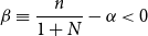 $\beta \equiv \dfrac {n}{1+N} - \alpha \lt 0$
(since
 $\alpha \gt 1$
and
 $n/(1+N) \lt 1$
). Rows (iii)–(iv) form a
 $2\times 2$
system in
 $(b, p_a)$
parameterized by
 $a$
. The determinant of this
 $2\times 2$
submatrix is:
 \begin{equation*} \delta _{34} = -\gamma \!\left (\frac {n}{\eta } + \frac {m}{D}\right ) + \frac {m^2\psi ^2}{D^2}\,. \end{equation*}
For
 $|\psi | \lt 1$
,
 $D \gt 0$
and all diagonal entries of
 $\mathbf{M}$
have definite signs, ensuring
 $\det \mathbf{M} \neq 0$
under the calibration. For
 $\psi \gt 1$
(substitute offsets),
 $D \lt 0$
, which changes the signs of the off-diagonal coupling terms but does not generically cause singularity; invertibility is verified numerically for the calibrated parameters.
Behavior of the price system
 $\mathbf{M}(x,y)\,\mathbf{v} = \mathbf{d}$
at boundary states

Table A1. Long description
A table summarizing the behavior of the price system at various boundary conditions. The table has four rows and four columns. The columns are labeled Boundary, Condition, det.M, and Economic interpretation. Row 1: Boundary is x = 1, Condition is n = 0, det.M is 0, Economic interpretation is All firms relocated; permit and offset markets inactive (zero demand). Rows (ii)(iii) collapse; a and b are undefined. Row 2: Boundary is y = 0, Condition is m = 0, det.M is 0, Economic interpretation is No farmer supplies offsets. System reduces to three equations in (p, a, p0); b is indeterminate. Row 3: Boundary is x = 0, y = 1, Condition is n = N, m = N0, det.M is not equal to 0, Economic interpretation is All firms stay home, all farmers offset. System generically non-singular.
In the numerical implementation,
 $\mathbf{M}(x,y)$
is inverted at each integration step of the replicator dynamics. MATLAB’s symbolic solver verifies invertibility over the relevant parameter space (see the code documentation).
Numerical verification
Under the baseline calibration (Table 2 in the main text), we evaluate
 $\mathbf{M}$
at representative interior points and verify positive prices. For instance, at the initial condition
 $(x_0, y_0) = (0.01, 0.2)$
with
 $\psi = 0$
:
 \begin{equation*} \mathbf{M} = \begin{pmatrix} 51 & -49.5 & 0 & 0 \\ 49.5 & -148.5 & 49.5 & 0 \\ 0 & 49.5 & -55.5 & 0 \\ 0 & 0 & 0 & 31 \end{pmatrix}, \quad \mathbf{d} = \begin{pmatrix} 150 \\ 50 \\ 0 \\ 25 \end{pmatrix}. \end{equation*}
This yields
 $(p, a, b, p_a) \approx (4.59,\; 1.70,\; 1.51,\; 0.81)$
, all strictly positive. The determinant is
 $\det \mathbf{M} \approx 4.94 \times 10^6 \neq 0$
, confirming invertibility. In the substitute case (
 $\psi = 3$
,
 $D = -8$
) at the same state, we obtain
 $\det \mathbf{M} \approx 3.00 \times 10^6$
and
 $(p, a, b, p_a) \approx (4.75,\; 1.87,\; 1.85,\; 0.86)$
, again all positive.
More broadly, the numerical implementation provides an implicit check on invertibility at every interior point: MATLAB’s symbolic solve() computes the closed-form price map
 $\mathbf{v}(x,y) = \mathbf{M}(x,y)^{-1}\mathbf{d}$
, which is then evaluated at each integration step by ode45. If
 $\det \mathbf{M} = 0$
were encountered along any trajectory, the price expressions would produce a division-by-zero error and the integrator would halt. No such failure occurs across all simulations reported in the paper, providing empirical confirmation that the price system remains non-singular along every realized trajectory in the interior of the state space.
Price positivity and the feasibility boundary
Although the matrix
 $\mathbf{M}$
is invertible over most of the interior, the resulting prices need not be positive everywhere. A systematic numerical sweep over the state space reveals that the permit price
 $a(x,y)$
changes sign along a critical locus. Under the baseline calibration with
 $\psi = 0$
, we find:
 \begin{equation*} a(x, y) = 0 \quad \text{at} \quad x \approx 0.66\,, \end{equation*}
independently of
 $y$
. For
 $x \gt 0.66$
, the permit price becomes negative, indicating that the cap is non-binding: so few firms remain in the jurisdiction that the fixed permit supply
 $Q$
exceeds total demand even without any abatement or offset. When
 $a \leq 0$
, the offset price
 $b$
is also non-positive, and the carbon markets become inactive.
This boundary has a natural economic interpretation: as carbon leakage increases, the demand for permits falls until the cap ceases to constrain production. Crucially, the stable equilibrium of the free entry–exit scenario lies precisely at this boundary:
 $[x^*, y^*] = [0.66, 0]$
, with
 $a = b = 0$
. The replicator dynamics drive the system to the point where the permit price vanishes, eliminating the cost differential between home and relocating firms. Beyond this point, further relocation yields no additional profit advantage, stabilizing the share.
For the policy scenarios (relocation cost, rationing), the stable equilibria lie in regions where
 $x$
is small (
 $x \leq 0.064$
), well within the positive-price domain. Thus, the feasibility constraint is binding only in the laissez-faire case, and precisely at its equilibrium.
A.4 Explicit replicator dynamics
Substituting the price solutions into the profit differentials from Section A.2 yields the replicator system
 $\dot {x} = F(x,y)$
,
 $\dot {y} = G(x,y)$
in closed form. We derive these expressions by sequential substitution through the price system.
Price solution: Sequential substitution
The almost block-triangular structure of
 $\mathbf{M}$
(Section A.3) enables a clean sequential solution. Define
 \begin{equation*} n \equiv (1-x)N, \quad m \equiv yN_a. \end{equation*}
Step 1. From the industrial goods Equation (A.38):
 \begin{equation} p(x,y) = \frac {\hat {p} + n\,a}{1 + N}. \end{equation}
Step 2. From the offset Equation (A.40), express
 $b$
in terms of
 $a$
and
 $p_a$
:
 \begin{equation} b = \frac {n\,D\,a + m\,\psi \,\eta \, p_a}{n\,D + m\,\eta }. \end{equation}
Step 3. Substitute Equations (A.45) and (A.46) into the permit market Equation (A.39) to solve for
 $a$
as a function of
 $(x, y, p_a)$
.
Step 4. The agricultural market Equation (A.41) provides the remaining relation linking
 $p_a$
to
 $(b, x, y)$
, closing the system.
For the general case (
 $\psi \gt 0$
), all four prices are coupled. Their closed-form expressions, while available, are rational functions of
 $(x, y)$
whose expanded forms span several lines and offer limited additional insight. In the numerical implementation, MATLAB’s symbolic solver computes these solutions at each integration step.
We therefore present the explicit replicator dynamics for the AOs case (
 $\psi = 0$
), which admits a particularly transparent factored form, and then summarize the structural differences in the substitute case (
 $\psi \gt 0$
).
Case
 $\psi = 0$
: Additional offsets
When
 $\psi = 0$
, the agricultural price decouples:
 \begin{equation} p_a = \frac {\hat {p}_a}{1 + N_a}\,, \end{equation}
which is constant, independent of
 $(x, y)$
. The remaining prices are determined by the
 $3 \times 3$
upper-left subsystem. Applying Cramer’s rule and factoring, the solutions take the form:
 \begin{align} a(x,y) &= \frac {3\bigl (Nx - \bar {n}\bigr )\bigl (5x - 3y - 5\bigr )}{(1-x)\,\Delta (x,y)}\,, \end{align}
 \begin{align} b(x,y) &= \frac {15\bigl (Nx - \bar {n}\bigr )}{\Delta (x,y)}\,, \end{align}
 \begin{align} p(x,y) &= \frac {50\bigl (25x - 24y - 25\bigr )}{\Delta (x,y)}\,, \end{align}
where
 \begin{equation*} \bar {n} \equiv \frac {Q(1+N)}{\hat {p}} = 17\,,\qquad \Delta (x,y) \equiv 250x^2 - 150xy + 10x - 309y - 260\,. \end{equation*}
Here
 $\bar {n}$
is the critical number of home firms at which the permit supply exactly exhausts demand under zero carbon prices, and
 $\Delta (x,y)$
is the (scaled) determinant of the
 $3 \times 3$
price subsystem.
Key structural feature. Both the permit price
 $a$
and the offset price
 $b$
share the common factor
 $(Nx - \bar {n})$
. They vanish simultaneously when
 \begin{equation} x = x^* \equiv \frac {\bar {n}}{N} = 1 - \frac {Q(1+N)}{N\hat {p}} = \frac {33}{50} = 0.66\,, \end{equation}
independently of
 $y$
. At this critical leakage share, the permit cap is exactly non-binding:
 $n^* = N(1-x^*) = \bar {n} = 17$
home firms demand precisely
 $Q = 50$
permits through production alone, rendering abatement and offset unnecessary (
 $z^* = c^* = 0$
). Since
 $a = b = 0$
, the home firm produces
 $q_h^* = p - 0 = p = q_r^*$
, yielding
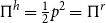 $\Pi ^h = \frac {1}{2}p^2 = \Pi ^r$
(with
 $R = 0$
). Both profit differentials vanish identically along the line
 $x = x^*$
for all
 $y \in [0,1]$
.
The explicit replicator system. Substituting the profit differentials (which depend on prices through Equations (A.48)–(A.50)) into the replicator equations yields:
 \begin{align} \dot {x} &= x(1-x)\,\Delta \Pi ^f (a(x,y),\, b(x,y),\, p(x,y) )\,, \\[-8pt]\nonumber\end{align}
 \begin{align} \dot {y} &= y(1-y)\,\frac {b(x,y)^2}{2}\,. \end{align}
For the agricultural sector, since
 $\psi = 0$
, the profit differential reduces to
 $\Delta \Pi ^\ell = b^2/2 \geq 0$
. Using Equation (A.49):
 \begin{equation} \dot {y} = y(1-y)\,\frac {225\,(Nx - \bar {n})^2}{2\,\Delta (x,y)^2} \geq 0\,, \end{equation}
with equality if and only if
 $y \in \{0, 1\}$
or
 $x = x^* = 0.66$
. This means that whenever
 $x \neq x^*$
and
 $y$
is interior, offset farmers are always entering the VCM (since offset production is always profitable under additional technologies). The share
 $y$
is monotonically increasing away from the critical line.
For the industrial sector,
 $\Delta \Pi ^f$
is a rational function of
 $(x,y)$
whose numerator is a polynomial of degree 4 in
 $x$
and degree 2 in
 $y$
:
 \begin{equation} \dot {x} = x(1-x)\,\frac {P_4(x,y)}{Q_6(x,y)}\,, \end{equation}
where
 $P_4$
and
 $Q_6$
denote the numerator and denominator polynomials respectively. The factor
 $(Nx - \bar {n})^2$
appears in
 $P_4$
, confirming that
 $\Delta \Pi ^f = 0$
along
 $x = x^*$
.
Corollary: The continuum of equilibria (Figure 1(a))
The shared factor
 $(Nx - \bar {n})$
in the price expressions immediately explains the “string of stable equilibria” observed in Figure 1(a) of the main text. When
 $\psi = 0$
and
 $R = 0$
:
-
1. Both
$\Delta \Pi ^f$
and
$\Delta \Pi ^\ell$
vanish along the entire line
$\{x^*\} \times [0,1]$
. -
2. The system
$(\dot {x}, \dot {y}) = (0, 0)$
is satisfied at every point
$(x^*, y)$
, creating a continuum (or manifold) of equilibria, not a discrete set. -
3. The economic mechanism is as follows: at
$x = x^*$
, carbon leakage has proceeded until the permit market clears at
$a = 0$
. With zero carbon prices, there is no cost differential between home and relocating firms (when
$R = 0$
), and no revenue for offset producers. The system is in a degenerate indifference state regardless of the VCM composition.


This manifold is structurally unstable: any perturbation that makes
 $a \neq b$
(such as
 $R \gt 0$
or rationing) breaks the degeneracy and selects discrete equilibria. This is precisely what occurs in the policy scenarios of Sections 3.5.2 and 3.5.3.
Case
 $\psi \gt 0$
: Substitute o
ffsets
When
 $\psi \gt 0$
, the agricultural and offset markets are coupled through
 $p_a$
, and the factorization structure breaks down. In particular:
-
• The agricultural price
$p_a(x,y)$
is no longer constant but depends on both shares. -
• The permit price
$a(x,y)$
does not generically share a common factor with
$b(x,y)$
. -
• As shown in Section A.2,
$\Delta \Pi ^\ell \lt 0$
for all interior prices when
$\psi \gt 1$
, so
$\dot {y} \leq 0$
: offset farmers always exit the VCM. -
• No continuum of equilibria arises; the equilibrium set is discrete.


The explicit price solutions for
 $\psi = 3$
are available in closed form but involve rational functions whose numerators are polynomials of degree 2 in both
 $x$
and
 $y$
; we omit their expanded expressions for brevity. The complete symbolic solutions are available in the MATLAB code, and all numerical results are computed from these closed forms.
Summary of the replicator system across scenarios
Table A2 summarizes the qualitative structure of the replicator dynamics across the three policy scenarios and two technology types.
Qualitative structure of the replicator dynamics.
 $x^{**}$
and
 $y^{**}$
denote scenario-specific interior equilibrium values from the numerical analysis

Table A2. Long description
A table comparing the qualitative structure of replicator dynamics across three policy scenarios and two technology types. The table has four rows and four columns. The columns are labeled Scenario, Sign of ψ, Equilibrium structure, and Carbon prices at eq. The rows are labeled with different scenarios: Free entry-exit, Relocation cost, and Rationing. Each row provides specific details for each scenario. Row 1: Free entry-exit, Sign of ψ is 0, Equilibrium structure is Continuum at x equals x asterisk, Carbon prices at eq is alpha equals b equals 0. Row 2: Free entry-exit, Sign of ψ is greater than 1, Equilibrium structure is Discrete: (x asterisk, 0), Carbon prices at eq is alpha equals b equals 0. Row 3: Relocation cost, Sign of ψ is 0, Equilibrium structure is Discrete: (0, 1), Carbon prices at eq is alpha, b greater than 0. Row 4: Relocation cost, Sign of ψ is greater than 1, Equilibrium structure is Discrete: (x asterisk, 0), Carbon prices at eq is alpha greater than 0, b equals 0. Row 5: Rationing, Sign of ψ is 0, Equilibrium structure is Discrete: (0, 1), Carbon prices at eq is alpha, b greater than 0. Row 6: Rationing, Sign of ψ is greater than 1, Equilibrium structure is Discrete: (0, x asterisk), Carbon prices at eq is alpha greater than 0, b greater than 0.
The table recaps the narrative of the numerical results of the main text. In the free entry–exit scenario (Figure 1(a)–(b)), the absence of a relocation cost leaves carbon leakage unchecked: the system converges to
 $x \approx 0.66$
, where permit prices vanish and carbon markets become inactive regardless of the offset technology. The introduction of a relocation cost
 $R \gt 0$
(Figure 2(a)–(b)) changes the dynamics fundamentally: the fixed cost reduces the relocation payoff at every
 $x$
, shifting the stable equilibrium leftward and sustaining positive carbon prices. Under additional technologies this is sufficient to support full VCM participation (
 $y = 1$
, Figure 2(a); under substitute technologies the negative sign of
 $\dot {y}$
still drives farmers out, but carbon leakage is substantially reduced (Figure 2(b)). Rationing (Figure 3(a)–(b)) provides further stabilization by fixing offset supply exogenously, which sustains a positive share of offsetters even when
 $\psi \gt 1$
, the only scenario yielding a stable interior equilibrium in the substitute case. Both relocation costs and rationing significantly improve welfare relative to free entry–exit (Table 3 of the main text), with the highest total welfare achieved under rationing with AOs. The sensitivity analyses corroborate these predictions across the parameter space: Figure 4 shows that the threshold
 $R$
required to eliminate carbon leakage is higher under substitute offsets, consistent with the stronger downward pressure on
 $y$
when
 $\psi \gt 1$
; Figure 5 confirms the bifurcation at
 $\psi = 1$
(Section A.1) across all three policy regimes, with the transition becoming less abrupt only under exogenous rationing (Figure 5(c)), where the policy mechanism partially compensates for the loss of concavity in the farmer’s problem; and Figures 6–9 verify robustness with respect to the permit cap
 $Q$
, the agricultural reserve price
 $\hat {p}_a$
, and the rationing coefficient
 $f$
.
A.5 Jacobian and stability analysis
The stability of each equilibrium
 $(x^*, y^*)$
is classified via the Jacobian matrix of the replicator system:
 \begin{equation} \mathbf{J}(x, y) = \begin{pmatrix} \dfrac {\partial F}{\partial x} & \dfrac {\partial F}{\partial y} \\ \dfrac {\partial G}{\partial x} & \dfrac {\partial G}{\partial y} \end{pmatrix}, \end{equation}
where
 $F(x,y) = x(1-x)\Delta \Pi ^f$
and
 $G(x,y) = y(1-y)\Delta \Pi ^\ell$
. The eigenvalues
 $\lambda _1, \lambda _2$
of
 $\mathbf{J}(x^*, y^*)$
determine local stability: the equilibrium is a stable node if both
 $\lambda _i \lt 0$
, an unstable node if both
 $\lambda _i \gt 0$
, and a saddle point if
 $\lambda _1$
and
 $\lambda _2$
have opposite signs. Equivalently, stability requires
 $\mathrm{tr}(\mathbf{J}) \lt 0$
and
 $\det (\mathbf{J}) \gt 0$
.
Structure of the Jacobian
Since the replicator equations have the multiplicative structure
 $\dot {x} = x(1-x)h_1(x,y)$
and
 $\dot {y} = y(1-y)h_2(x,y)$
, the Jacobian at boundary equilibria simplifies considerably. At a corner
 $(x^*, y^*) \in \{0,1\} \times \{0,1\}$
:
 \begin{equation} \mathbf{J}(x^*, y^*) = \begin{pmatrix} (1 - 2x^*)\Delta \Pi ^f\big |_{(x^*,y^*)} & 0 \\ \star & (1 - 2y^*)\Delta \Pi ^\ell \big |_{(x^*,y^*)} \end{pmatrix}, \end{equation}
which is (block-)triangular. The eigenvalues are thus the diagonal entries:
 \begin{equation*} \lambda _1 = (1-2x^*)\Delta \Pi ^f(x^*,y^*), \qquad \lambda _2 = (1-2y^*)\Delta \Pi ^\ell (x^*,y^*)\,. \end{equation*}
At
 $x^* = 0$
:
 $\lambda _1 = \Delta \Pi ^f$
; at
 $x^* = 1$
:
 $\lambda _1 = -\Delta \Pi ^f$
. Similarly for
 $y^*$
. This means that the sign of each profit differential at a corner directly determines the stability in the corresponding direction: positive
 $\Delta \Pi ^f$
at
 $(0, \cdot )$
pushes
 $x$
upward (firms relocate), contributing an unstable eigenvalue.
At interior equilibria, the full Jacobian must be computed, as the off-diagonal terms are generally nonzero. All Jacobians are computed symbolically in MATLAB and evaluated numerically at each equilibrium.
Results by scenario
Table A3 reports the eigenvalues and stability classification at each equilibrium for all six scenario–technology combinations. The column labels are: Sc. = scenario,
 $\psi$
= switching cost,
 $R$
= relocation cost, Eq. = equilibrium point,
 $\lambda _1, \lambda _2$
= eigenvalues, Class. = stability classification.
Eigenvalue-based stability classification at each equilibrium under the baseline calibration (Table 2). Eigenvalues rounded to two decimal places

Table A3. Long description
The table presents eigenvalue-based stability classifications for various scenarios and policies. It consists of six rows and eight columns. The columns are labeled as Sc., Policy, ψ, Eq. (x*, y*), λ1, λ2, and Class. The rows are labeled with scenario numbers from 1 to 6. Each row provides detailed information on the policy, switching cost (ψ), equilibrium points (x*, y*), eigenvalues (λ1, λ2), and stability classification. For example, Row 1: Sc. 1, Policy Free entry-exit, ψ 0, Eq. (0, 0), λ1 +5.53, λ2 +1.81, Class. Unstable. Row 2: Sc. 2, Policy Free entry-exit, ψ 3, Eq. (0, 0), λ1 +5.53, λ2 -0.02, Class. Stable. Row 3: Sc. 3, Policy Relocation cost, ψ 0, Eq. (0, 0), λ1 +0.53, λ2 +1.81, Class. Unstable. Row 4: Sc. 4, Policy Relocation cost, ψ 3, Eq. (0, 0), λ1 +0.53, λ2 -0.02, Class. Stable. Row 5: Sc. 5, Policy Rationing, ψ 0, Eq. (0, 0), λ1 +0.53, λ2 +0.58, Class. Unstable. Row 6: Sc. 6, Policy Rationing, ψ 3, Eq. (0, 0), λ1 +0.53, λ2 +0.27, Class. Unstable. The table provides a comprehensive comparison of stability classifications across different scenarios and policies.
 $^\dagger$
One zero eigenvalue: The equilibrium lies on the continuum
 $\{x^*\} \times [0,1]$
(see Section A.4). The
 $x$
-direction is attracting (
 $\lambda _1 \lt 0$
), while the
 $y$
-direction is neutral (
 $\lambda _2 = 0$
).
Discussion
Several features of the stability results merit comment:
-
1. Free entry–exit with
$\psi = 0$
: the non-hyperbolic manifold. At
$(0.66, 0)$
and
$(0.66, 1)$
, one eigenvalue is zero because the equilibrium sits on the continuum identified in Section A.4. The Jacobian isThe system is attracting in the
\begin{equation*} \mathbf{J}(0.66, y) = \begin{pmatrix} -3.43 & 0 \\ 0 & 0 \end{pmatrix} \qquad \text{(approximately, for any } y\text{)}. \end{equation*}
$x$
-direction but neutral in
$y$
. The trajectory converges to the line
$x = 0.66$
but does not select a unique
$y^*$
; the final
$y$
depends on the initial conditions. This non-hyperbolicity is structurally unstable: any
$R \gt 0$
or rationing breaks it.
-
2. Effect of relocation costs on
$\lambda _1$
. Comparing Scenarios 1 and 3 in
$(0, 0)$
: the first eigenvalue drops from
$+5.53$
to
$+0.53$
. The relocation cost
$R$
directly reduces
$\Delta \Pi ^f$
at
$x = 0$
, weakening the incentive to relocate. At
$(0, 1)$
, this pushes
$\lambda _1$
from
$+3.92$
(unstable) to
$-1.08$
(stable), flipping the stability of the full-participation equilibrium. -
3. Substitute offsets (
$\psi \gt 1$
) yield
$\lambda _2 \lt 0$
in the
$y$
-direction. Since
$\Delta \Pi ^\ell \lt 0$
whenever
$\psi \gt 1$
(Section A.2), the
$y$
-eigenvalue at any
$(x^*, 0)$
boundary is negative, making
$y = 0$
attracting. This is the analytical confirmation that substitute offsets drive VCM extinction without policy support. -
4. Rationing with substitute offsets (Scenario 6). This is the only scenario that produces a stable interior equilibrium at
$(0.037, 0.216)$
: both eigenvalues are strictly negative (
$-0.39, -0.17$
). The combination of CBAM and rationing maintains a small but positive share of VCM even with switching costs, as exogenous offset demand guarantees revenue for farmers.


A.6 Numerical implementation
Population shares
 $(x,y)$
evolve via the replicator dynamics, while the prices
 $(p, a, b, p_a)$
are not state variables but are determined instantaneously by the linear market-clearing system
 $\mathbf{M}(x,y)\,\mathbf{v} = \mathbf{d}$
(Section A.3). Since this system is linear in prices, its solution
 $\mathbf{v}(x,y) = \mathbf{M}(x,y)^{-1}\mathbf{d}$
is a smooth rational map wherever
 $\det \mathbf{M} \neq 0$
, which holds throughout the interior of the state space (Section A.3). Substituting back yields a well-posed ODE system
 $\dot {x} = F(x,y)$
,
 $\dot {y} = G(x,y)$
with smooth right-hand side, to which standard existence and uniqueness results apply. In the numerical implementation, MATLAB’s symbolic solver computes the closed-form price map once, converts
 $F$
and
 $G$
to function handles, and passes the resulting ODE to the ode45 integrator. In the numerical simulations, the system is integrated as follows:
-
1. At each integration step
$t$
, given current shares
$(x(t), y(t))$
, assemble the coefficient matrix
$\mathbf{M}(x(t), y(t))$
. -
2. Solve the linear system
$\mathbf{M}\mathbf{v} = \mathbf{d}$
for prices. -
3. Compute the profit differentials
$\Delta \Pi ^f$
and
$\Delta \Pi ^\ell$
from the solved prices. -
4. Evaluate the right-hand side
$(F, G)$
and advance
$(x, y)$
using MATLAB’s ode45 solver.


Appendix B: Monopolistic competition robustness check
Let
 $\mu \geq 0$
denote the markup parameter, with
 $\alpha \equiv 1+\mu$
. The only modified FOCs are the output decisions of industrial firms:
 \begin{equation} q_h^* = \frac {p - a}{\alpha }\,,\qquad q_r^* = \frac {p}{\alpha }\,. \end{equation}
All other optimal quantities (
 $z^*$
,
 $c^*$
,
 $q_o^*$
,
 $s^*$
,
 $q_a^*$
) are unchanged.
Modified price system. Substituting Equation (B.58) into the market-clearing conditions yields a linear system
 $\mathbf{M}\,\mathbf{v} = \mathbf{d}$
with
 $\mathbf{v} = (p,\,a,\,b,\,p_a)^\top$
. Only Rows 1–2 are affected:
 \begin{align} \text{(Commodity):}\quad & (\alpha + N)\,p - N_h\,a = \hat {p}\,\alpha\\[-6pt]\nonumber \end{align}
 \begin{align} \text{(Permits):}\quad & \frac {N_h}{\alpha }\,p - N_h\!\left (\frac {1}{\alpha }+\frac {1}{\theta }+\frac {1}{\eta }\right )a + \frac {N_h}{\eta }\,b = Q \end{align}
where
 $N_h=(1-x)N$
. The offset and agricultural market equations (Rows 3–4) are identical to the baseline. The system remains linear in prices and invertible under the same conditions as in the competitive case, with
 $\alpha$
replacing
 $1$
in the relevant coefficients.
Modified profit differential. Substituting the optimal quantities into the profit functions:
 \begin{align} \Pi ^r\big |^* &= \frac {(1+2\mu )\,p^2}{2\alpha ^2} - R\,,\\[-6pt]\nonumber \end{align}
 \begin{align} \Pi ^h\big |^* &= \frac {(1+2\mu )(p-a)^2}{2\alpha ^2} + \frac {a^2}{2\theta } + \frac {(a-b)^2}{2\eta }\,. \end{align}
The industrial profit differential is therefore:
 \begin{equation} \Delta \Pi ^f = m(\mu )\cdot a(2p-a) - \frac {a^2}{2\theta } - \frac {(a-b)^2}{2\eta } - R\,, \end{equation}
where
 \begin{equation} m(\mu ) \equiv \frac {1+2\mu }{2(1+\mu )^2} \end{equation}
is a markup factor satisfying
 $m(0) = 1/2$
(recovering the competitive baseline) and
 $m'(\mu ) = -\mu /(1+\mu )^3 \lt 0$
for
 $\mu \gt 0$
. The agricultural profit differential
 $\Delta \Pi ^\ell$
retains its baseline form;
 $\mu$
enters only indirectly through the equilibrium prices
 $b$
and
 $p_a$
.
Replicator dynamics. The dynamical system
 $\dot {x}=x(1-x)\,\Delta \Pi ^f$
,
 $\dot {y}=y(1-y)\,\Delta \Pi ^\ell$
has the same structure as the baseline.
Numerical results. We sweep
 $\mu$
from
 $0$
(perfect competition) to
 $2$
(corresponding to
 $\sigma = 1.5$
) across all six policy scenarios. Table A4 reports the stable equilibrium
 $(x^*,\,y^*)$
at three representative values. The main findings are as follows.
Stable equilibria under monopolistic competition

Table A4. Long description
The table presents stable equilibria under monopolistic competition for six different scenarios and three values of mu (0, 0.5, 1.0). It has six rows and four columns. The columns are labeled Scenario, mu = 0, mu = 0.5, and mu = 1.0. Each column under mu values contains sub-columns labeled (x*, y*). Row 1: Free, add. (x*, y*): mu = 0 (0.66, any), mu = 0.5 (0.66, any), mu = 1.0 (0.65, any). Row 2: Free, comp. (x*, y*): mu = 0 (0.66, 0), mu = 0.5 (0.66, 0), mu = 1.0 (0.65, 0). Row 3: Reloc., add. (x*, y*): mu = 0 (0, 1), mu = 0.5 (0.006, 1), mu = 1.0 (0.066, 1). Row 4: Reloc., comp. (x*, y*): mu = 0 (0.048, 0), mu = 0.5 (0.210, 0), mu = 1.0 (0.281, 0). Row 5: Rat., add. (x*, y*): mu = 0 (0, 1), mu = 0.5 (0.130, 1), mu = 1.0 (0.187, 1). Row 6: Rat., comp. (x*, y*): mu = 0 (0.037, 0.22), mu = 0.5 (0.202, 0.11), mu = 1.0 (0.275, 0.065).
 $^\dagger$
Non-hyperbolic manifold along
 $x\approx 0.66$
;
 $y^*$
depends on initial conditions.
In all scenarios, the qualitative stability classification is preserved: the number and type (stable node, saddle, source) of equilibria remain the same, and the basin-of-attraction structure is unchanged. The stable equilibrium shifts smoothly with
 $\mu$
. Carbon leakage
 $x^*$
increases moderately, consistent with
 $m'(\mu )\lt 0$
reducing each firm's compliance cost advantage, while VCM participation
 $y^*$
is largely unaffected. A bifurcation occurs in Scenarios 3 and 5 (AOs with relocation costs): at
 $\mu =0$
the corner
 $(0,\,1)$
is stable, but for
 $\mu \gt \mu ^*(R)$
(the bifurcating
 $\mu$
given a value of
 $R$
) a small positive
 $x^*$
emerges on the
 $y=1$
boundary. At the calibrated baseline
 $R=5$
, we find
 $\mu ^*\approx 0.33$
(Sc. 3) and
 $\mu ^*\approx 0.07$
(Sc. 5). Crucially,
 $y^*=1$
is preserved. VCM participation survives the markup. The critical
 $\mu ^*$
increases with
 $R$
, and for
 $R \geq 5.7$
the competitive equilibrium is robust to any realistic markup (
 $\mu ^* \gt 5$
, i.e.,
 $\sigma \lt 1.2$
). The “string of equilibria” along
 $x \approx 0.66$
in Scenario 1 (free entry, additional) persists at all
 $\mu$
values, confirming that this non-hyperbolic manifold is a structural feature of the additivity assumption (
 $\psi =0$
), not an artifact of the competitive market structure.
In summary, monopolistic competition acts as a smooth perturbation of the competitive benchmark. The central policy rankings of the main text are preserved: relocation costs and rationing continue to outperform free entry–exit, and AOs remain more competitive than substitute ones. The only qualitative change is a modest re-emergence of carbon leakage in Scenarios 3 and 5 at high markups. This reinforces rather than undermines the case for combining CBAM with VCM support, as voluntary market participation is sustained throughout.

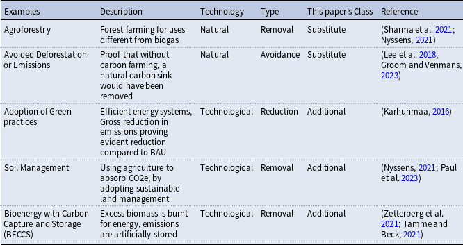
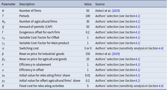

 x
 y
 ψ=0
 ψ>0

 x
 y
 ψ=0
 ψ>0

 x
 y
 ψ=0
 ψ>0
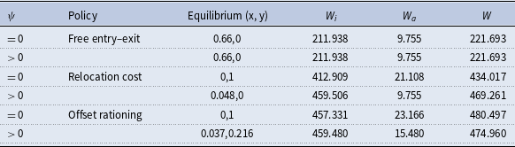
 ψ>0
 ψ=0

 R

 ψ

 Q

 p^a

 f

 f
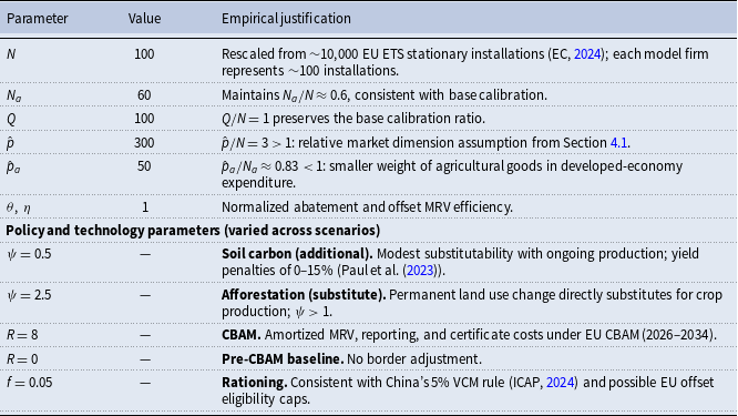


 x∗
 y∗
 y∗
 x≈0.66
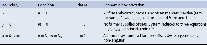
 M(x,y)v=d
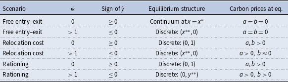
 x∗∗
 y∗∗
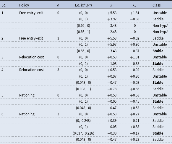
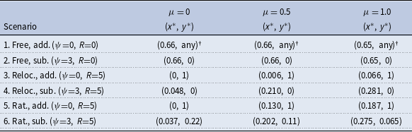


 Open access

