1 Introduction
The shock-wave/boundary layer interaction which occurs on the upper side of a wing can, at high Mach number and/or high angle of attack, induce a massive flow separation which can lead to instability. This instability is characterised by a shock location oscillation. This phenomenon is known as ‘buffet’ and can further lead to structural vibrations (‘buffeting’). Transonic buffet results in lift and drag variations and consequently vibrations that greatly affect the aircraft aerodynamics and, as such, limits the aircraft flight envelope. This phenomenon presenting an industrial interest, it has therefore been the subject of numerous studies in the past (Pearcey Reference Pearcey1958; McDevitt & Okuno Reference McDevitt and Okuno1985).
In the turbulent flow regime, on a two-dimensional profile, the shock oscillates at low frequency (
 $St=f\cdot c/U_{\infty }\simeq 0.06{-}0.07$
, where
 $St$
is the Strouhal number,
 $f$
the shock oscillation frequency,
 $c$
the chord length and
 $U_{\infty }$
the free-stream velocity) with a large amplitude (typically 20 % of chord) (see Jacquin et al.
Reference Jacquin, Molton, Deck, Maury and Soulevant2009, for example). Lee (Reference Lee1990, Reference Lee2001) explains the turbulent two-dimensional (2-D) transonic buffet as a self-sustained loop based on the coupling between the shock and the trailing edge through pressure waves. The shock wave generates pressure waves which propagate downstream inside the boundary layer; these waves are diffracted at the trailing edge, generating new waves that travel back upstream outside the boundary layer, up to the shock. These waves create new pressure waves and close the loop. More recently, Crouch et al. (Reference Crouch, Garbaruk, Magidov and Travin2009b
) and Sartor, Mettot & Sipp (Reference Sartor, Mettot and Sipp2014) explained the turbulent 2-D transonic buffet as an unstable global mode. At high Mach number or angle of attack, the analysis of the eigenvalues of the Jacobian of the Navier–Stokes operator exhibit one single eigenvalue with a positive real part at the buffet frequency leading to an amplification of the perturbations.
Today, laminarity is unanimously seen as one key to reach the objective of a 75 % reduction in fuel consumption and carbon dioxide in 2050. On civil aircraft, friction drag contributes to 50 % of total drag and 40 % of this friction drag comes from the wings. Potential aircraft drag reduction of 10 % by reducing the wing drag by 25 % using laminarity is foreseen. Hence, laminarity offers new aerodynamics challenges and in particular one question which arises is: is laminar transonic buffet stronger than the turbulent one in terms of pressure fluctuations or not? This question is of fundamental importance to determine the flight envelope limits in the laminar flow regime. Unfortunately, the 2-D transonic buffet phenomenon has received much less attention in the laminar case than in the turbulent one. Dor et al. (Reference Dor, Mignosi, Seraudie and Benoit1989) did not observe shock oscillations in buffet conditions at
 $M=0.75$
,
 $\unicode[STIX]{x1D6FC}=3^{\circ }$
,
 $Re_{c}=3\times 10^{6}$
. Just a strong increase of the pressure fluctuation level was observed without any particular frequency. More recently, the same airfoil has been tested by Bur, Brion & Molton (Reference Bur, Brion and Molton2014). Instead of a low-frequency peak at
 $St\simeq 0.06{-}0.07$
, a high-frequency peak around
 $St=0.9$
, one order of magnitude larger than in the turbulent case, has been observed in the pressure spectra at
 $M=0.73$
,
 $\unicode[STIX]{x1D6FC}=3.5^{\circ }$
,
 $Re_{c}=3\times 10^{6}$
. The presence of a very thin recirculation bubble at the shock foot was reported and it is assumed that this bubble dynamics is the most likely cause of the pressure peak at high frequency.
To improve the knowledge on laminar transonic buffet, a European project named BUTERFLI was launched in 2013. In particular, wind tunnel tests on a laminar airfoil have been performed in ONERA’s S3Ch wind tunnel. The experimental set-up allowed for varying the Mach number, the angle of attack and the state of the boundary layer upstream of the shock (laminar or turbulent) depending on the presence of artificial tripping. In the turbulent case at
 $M=0.735$
,
 $\unicode[STIX]{x1D6FC}=4^{\circ }$
,
 $Re_{c}=3\times 10^{6}$
, Brion et al. (Reference Brion, Dandois, Abart and Paillart2017) reported a low-frequency peak in the wall pressure spectra at approximately 75 Hz (
 $St=0.07$
) in agreement with Jacquin et al. (Reference Jacquin, Molton, Deck, Maury and Soulevant2009). In the laminar case (same flow conditions without tripping), a peak at a much higher frequency (approximately 1130 Hz or
 $St=1$
) was observed as in Bur et al. (Reference Bur, Brion and Molton2014).
In the framework of the European TFAST project, Davidson & Babinsky (Reference Davidson and Babinsky2016) have studied the interaction of a shock wave and laminar boundary layer on a flat plate and a laminar airfoil for
 $0.7<M<0.72$
,
 $\unicode[STIX]{x1D6FC}=0^{\circ }$
,
 $1.8\times 10^{6}<Re_{c}<2.6\times 10^{6}$
. On the airfoil case, they reported Strouhal numbers between 0.12 and 0.16 depending on the Mach number. These results differ from the literature on two points. First, in the tripped case, the Strouhal number is larger than values usually found in the literature (0.14–0.15 instead of 0.06–0.09 in McDevitt & Okuno (Reference McDevitt and Okuno1985), 0.06–0.08 in Benoit & Legrain (Reference Benoit and Legrain1987),
 $\simeq 0.09$
in Lee & Tang (Reference Lee and Tang1988), 0.06–0.07 in Jacquin et al. (Reference Jacquin, Molton, Deck, Maury and Soulevant2009), 0.07–0.1 in Zhao et al. (Reference Zhao, Ren, Gao, Xiong, Liu and Luo2013) and 0.07–0.08 in Kouchi et al. (Reference Kouchi, Yamaguchi, Koike, Nakajima, Sato, Kanda and Yanase2016)). Secondly, contrary to Bur et al. (Reference Bur, Brion and Molton2014) and Brion et al. (Reference Brion, Dandois, Abart and Paillart2017), the Strouhal number does not depend on the state of the turbulent boundary layer. This is attributed to the fact that the separation bubble at the shock foot is very thin and has little impact on the interaction.
On the numerical side, there are very few studies on the laminar transonic buffet phenomenon on airfoils. Memmolo, Bernardini & Pirozzoli (Reference Memmolo, Bernardini and Pirozzoli2016) have performed a large-eddy simulation of transonic buffet in laminar conditions. Two main peaks were identified: a low-frequency peak at
 $St\simeq 0.1$
concentrated around the mean shock position associated with transonic buffet; and a secondary peak at higher frequency (
 $St\simeq 1$
) attributed to a Kelvin–Helmholtz (K–H) vortex shedding process in the separation. So, in this simulation, both the turbulent (low frequency) and laminar (high frequency) transonic buffet dynamics are retrieved.
Aside from the literature on transonic buffet on airfoils, studies on oblique shock-wave boundary layer interaction (SWBLI) on a flat plate are more numerous since this is an academic configuration representative of aeronautical applications like turbine blades, air inlets of supersonic jets or rockets nozzles. Like the transonic buffet literature on airfoils, shock-wave interaction with a laminar boundary layer has been far less studied than in the turbulent regime. Over the last decade, the low-frequency unsteadiness observed in the SWBLI has been widely studied both experimentally by Dupont, Haddad & Debiève (Reference Dupont, Haddad and Debiève2006), Ganapathisubramani, Clemens & Dolling (Reference Ganapathisubramani, Clemens and Dolling2007) and numerically by Wu & Martin (Reference Wu and Martin2008), Touber & Sandham (Reference Touber and Sandham2011) and Agostini et al. (Reference Agostini, Larchevêque, Dupont, Debiève and Dussauge2012) among others. However, the origin of this low-frequency unsteadiness is still not clear. On the one hand, this is explained by the interaction of the shock foot with turbulent structures of the incoming upstream boundary layer (Ganapathisubramani et al.
Reference Ganapathisubramani, Clemens and Dolling2007). On the other hand, the unsteadiness is explained by an intrinsic mechanism of the SWBLI (Dupont et al.
Reference Dupont, Haddad and Debiève2006; Touber & Sandham Reference Touber and Sandham2011). Nevertheless, this SWBLI differs from the present laminar transonic buffet on two points. First, the Strouhal numbers based on the separation length and the velocity upstream of the shock are much lower (
 $St_{L}\simeq 0.02{-}0.05$
, see figure 3 in Dussauge, Dupont & Debiève (Reference Dussauge, Dupont and Debiève2006)) than for the laminar transonic buffet phenomenon (
 $St_{L}=0.13$
in Brion et al. (Reference Brion, Dandois, Abart and Paillart2017)). Secondly, the low-frequency unsteadiness in the oblique SWBLI is characterised by a large bump in the power spectra (see figure 4 in Dussauge et al. (Reference Dussauge, Dupont and Debiève2006) for example) rather than a peak in the laminar transonic buffet case (see figure 10b in Brion et al. (Reference Brion, Dandois, Abart and Paillart2017)). Concerning the interaction of an oblique shock wave with a laminar boundary layer, this has just started to receive some attention recently (Sansica, Sandham & Hu Reference Sansica, Sandham and Hu2014, Reference Sansica, Sandham and Hu2016; Bur & Garnier Reference Bur and Garnier2016; Larchevêque Reference Larchevêque2016). As in the turbulent case, a low-frequency unsteadiness has also been observed numerically at
 $St_{L}=0.04$
by Sansica et al. (Reference Sansica, Sandham and Hu2016),
 $St_{L}=0.025$
to 0.06 depending on the bubble size in Larchevêque (Reference Larchevêque2016) and two bumps at
 $St_{L}=0.09$
to 0.31 in Bur & Garnier (Reference Bur and Garnier2016). Except the last
 $St_{L}$
at 0.31 which is not too far from the laminar transonic buffet one at 0.13 in (Brion et al.
Reference Brion, Dandois, Abart and Paillart2017), all Strouhal numbers are close to the ones found in the turbulent regime and two to five times smaller than the one found in Brion et al. (Reference Brion, Dandois, Abart and Paillart2017). Nevertheless, in both turbulent or laminar SWBLI, the low-frequency unsteadiness has been identified as a separation bubble breathing phenomenon with vortices shed downstream. Non-dimensionalising by the displacement thickness at the separation
 $\unicode[STIX]{x1D6FF}_{S}^{\ast }$
instead of the interaction length does not improve the Strouhal number agreement between oblique SWBLI and laminar transonic buffet. However, it must be pointed out that the flow configurations are different: the incident shock is oblique and not normal like on an airfoil and its location is not free but fixed by the shock generator.
In the subsonic regime, laminar separation bubbles (LSB) are encountered in many applications like for example airfoils near stall, turbine blades, etc. They play a major role in the dynamic stall of helicopter blades but also in the static stall of wings or wind turbine blades. Bubbles are classified into two main types (Owen & Klanfer Reference Owen and Klanfer1953): ‘short’ bubbles when the bubble length is of the order of 1 % of the aerofoil chord and
 $10^{2}\unicode[STIX]{x1D6FF}_{S}^{\ast }$
where
 $\unicode[STIX]{x1D6FF}_{S}^{\ast }$
is the displacement thickness at separation, and ‘long’ bubbles when the length is of the order of
 $10^{4}\unicode[STIX]{x1D6FF}_{S}^{\ast }$
. Yang & Voke (Reference Yang and Voke2001) reported
 $St_{L}$
between 0.52 and 1.14 (or
 $St_{\unicode[STIX]{x1D6FF}_{S}^{\ast }}=0.005$
to 0.011) for the bubble bursting phenomenon. In Laurent et al. (Reference Laurent, Mary, Gleize, Lerat and Arnal2012),
 $St_{L}$
is equal to 2.7 (
 $St_{\unicode[STIX]{x1D6FF}_{S}^{\ast }}=0.12$
). Marquillie & Ehrenstein (Reference Marquillie and Ehrenstein2003) have studied numerically the effect of the Reynolds number on the flow at the rear of a two-dimensional bump mounted on a flat plate. Two instabilities have been identified: a convective one corresponding to the K–H instability in the shear layer at
 $St_{\unicode[STIX]{x1D6FF}_{S}^{\ast }}=0.04$
and an absolute one which appears above a critical Reynolds number at
 $St_{\unicode[STIX]{x1D6FF}_{S}^{\ast }}=0.005$
corresponding to the vortex shedding.
The present paper presents results from a large-eddy simulation (LES) in the same flow conditions than the wind tunnel tests in Brion et al. (Reference Brion, Dandois, Abart and Paillart2017). In laminar conditions, the separation bubble at the shock foot is very thin and consequently, it is very difficult to perform particle image velocimetry for example close to the wall where there are potentially laser sheet reflections. Compared to the wind tunnel tests, the numerical simulations allow analysing with great spatial and temporal resolution the separation bubble dynamics which is the key to understanding the laminar transonic buffet phenomenon.
The article is organised as follows. In § 2, the flow configuration is presented. The key elements of the numerical method, computational grid and boundary conditions are described in § 3. In § 4, the results from the large-eddy simulation are presented. The bubble dynamics is analysed thanks to phase-averaged flow fields and wall pressure spectra. Lastly, to explain the laminar transonic buffet frequency, possible physical mechanisms are discussed in § 5.
2 Flow configuration
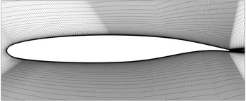
The geometry consists of the OALT25 supercritical laminar airfoil (see figure 1) with a chord length
 $c$
equal to 0.23 m. The trailing-edge thickness is equal to 0.5 % of chord.
Experimentally, several Mach numbers have been tested between
 $M=0.7$
and 0.79 and also angles of attack between 1.5 and
 $4^{\circ }$
corresponding to free-stream conditions before and after transonic buffet onset. It has been checked by using an infrared camera that the flow is laminar up to the shock foot (see Brion et al.
Reference Brion, Dandois, Abart and Paillart2017 for more details on the experiment). For the present LES, one test case in laminar transonic buffet conditions has been selected in the database:
 $M=0.735$
,
 $\unicode[STIX]{x1D6FC}=4^{\circ }$
,
 $Re_{c}=2.8\times 10^{6}$
.
The coordinate system is the following:
 $x$
is oriented in the streamwise direction,
 $y$
is vertical and
 $z$
is in the spanwise direction. The origin is located at the airfoil leading edge.
OALT25 airfoil (partial view, one point over two plotted).

3 Numerical method
The ONERA’s FastS solver has been used to solve the compressible Navier–Stokes equations. For LES, the filtered equations are obtained using the formalism developed by Vreman (Reference Vreman1995). No subgrid-scale model is used so it is an implicit LES simulation (ILES). The spatial scheme is the one proposed by Mary & Sagaut (Reference Mary and Sagaut2002). It is based on a modification of the AUSM+(P) scheme (see Edwards & Liou Reference Edwards and Liou1998) which is second-order accurate. The time integration is carried out by means of the second-order accurate backward scheme of Gear. More details about the numerical method are available in Péchier, Guillen & Gayzac (Reference Péchier, Guillen and Gayzac2001). The time step is taken equal to 0.0001
 $c/U_{\infty }$
. The resulting nonlinear system is solved iteratively at every time step with 30 sub-iterations, resulting in a reduction of the residuals of approximately one order of magnitude. The simulated physical time corresponds to approximately
 $100c/U_{\infty }$
.
Figure 1 shows the LES mesh. Since the flow is laminar up to the shock foot, the mesh density is lower in the streamwise direction upstream of the shock. The grid refinement is concentrated at the shock foot in the shear layer where laminar/turbulent transition occurs, downstream of the shock and on the pressure side since the flow is tripped at
 $x/c=7\,\%$
. On the lower side, the laminar/turbulent transition is triggered thanks to a small step of a height roughly equal to the carborundum band one used in the wind tunnel tests. The spanwise extent of the computational domain is equal to 10 % of chord, or 23 separation bubble heights. The effect of the spanwise extent of the computational domain has been investigated in Larchevêque (Reference Larchevêque2016) using the same solver on the case of SWBLI with a laminar incoming boundary layer, so a case similar to the present one. In this study, two span extents of 16 and 32 separation bubble heights were simulated with identical results for the skin friction and wall pressure distributions (see their figure 1c,d). In the present paper, the spanwise extent of the computational domain is 23 separation bubble heights. The cell sizes are on the upper side, downstream of the shock
 $x^{+}=25$
,
 $y^{+}=1$
,
 $z^{+}=5$
(close to a direct numerical simulation (DNS) resolution and better than usual LES resolutions) and on the lower side
 $x^{+}=46$
,
 $y^{+}=1$
,
 $z^{+}=15$
(classical LES resolution). The effect of the grid resolution on the turbulence statistics has not been assessed on the present case but on a similar one (transitional separation bubble, see Laurent et al. (Reference Laurent, Mary, Gleize, Lerat and Arnal2012)). Five grid densities were compared and the results were considered as converged on the 60 million cell grid which had a resolution
 $x^{+}=27$
,
 $y^{+}=1$
,
 $z^{+}=5$
, close the present one on the suction side. The grid is stretched with a ratio of 5 % in the wall-normal direction and in the streamwise direction downstream of the trailing edge. There are 3585 cells around the airfoil, 189 in the wall-normal direction and 718 in the spanwise direction. The total mesh size is
 $400\times 10^{6}$
cells.
Far-field boundary conditions are imposed 50 chords away from the airfoil. An adiabatic no-slip boundary condition is imposed on the walls and periodic boundary conditions in the
 $z$
direction.
4 Results analysis
This section presents results of the LES simulation first on an instantaneous field then on the time-averaged one and finally on phase-averaged ones. Signal processing tools are then used to underline the main features of the laminar transonic buffet phenomenon.
4.1 Instantaneous field analysis
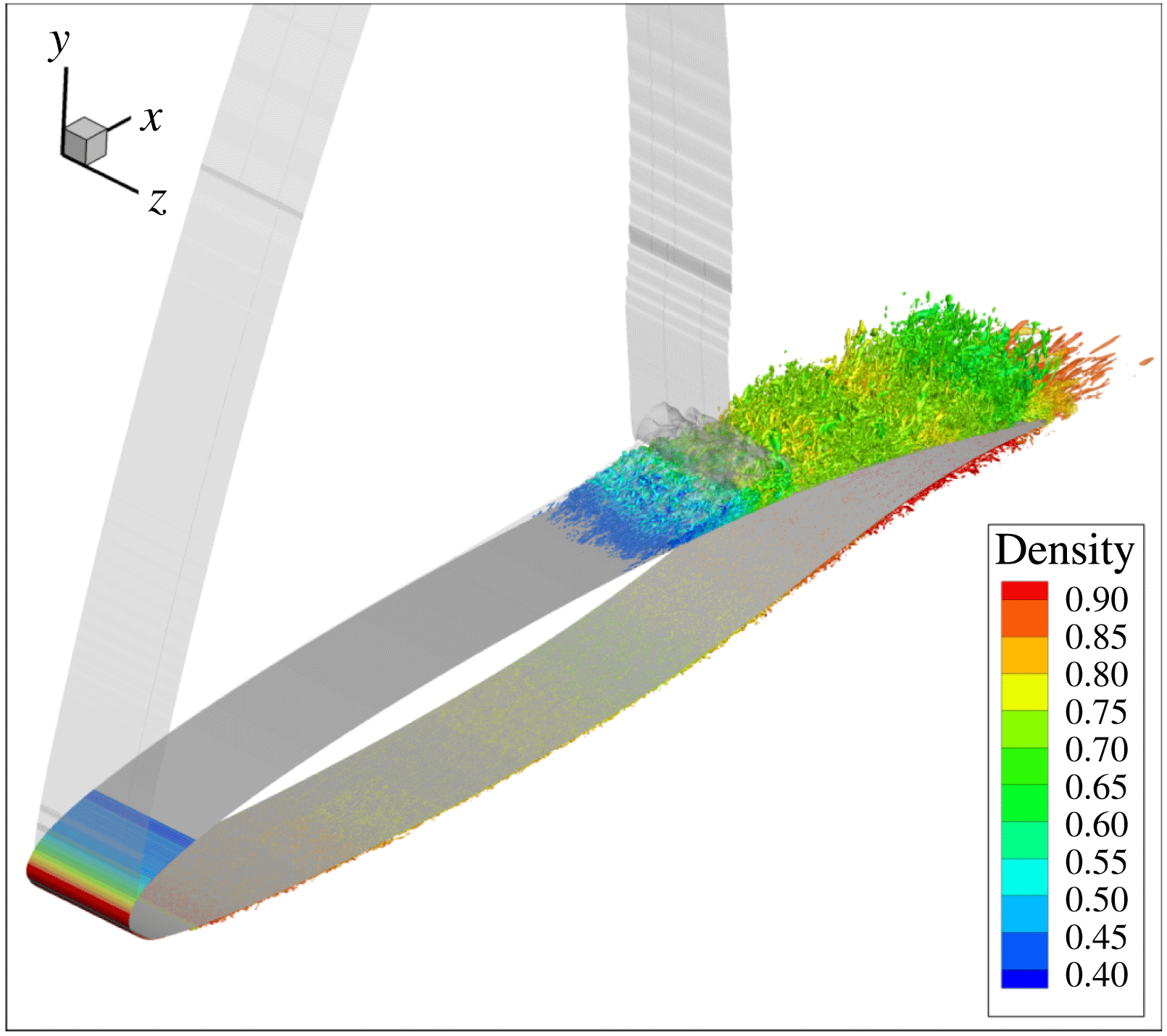
Figure 2 shows a
 $Q$
-criterion isosurface (in red) and the isosurface
 $M=1$
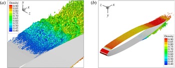
(translucent). Since the flow is laminar up to the shock foot, there are no turbulent structures in the boundary layer upstream of the shock. The laminar/turbulent transition occurs in the shear layer of the separation bubble at the shock foot. Then, downstream of the shock, the flow is turbulent. Figure 3 shows two zooms on the shock foot and on the pressure side.
 $Q$
-criterion isosurface
 $Q\cdot c^{2}/U_{\infty }^{2}=5000$
coloured by the density with isosurface
 $M=1$
(translucent) and wall surface (in grey).

From the
 $Q$
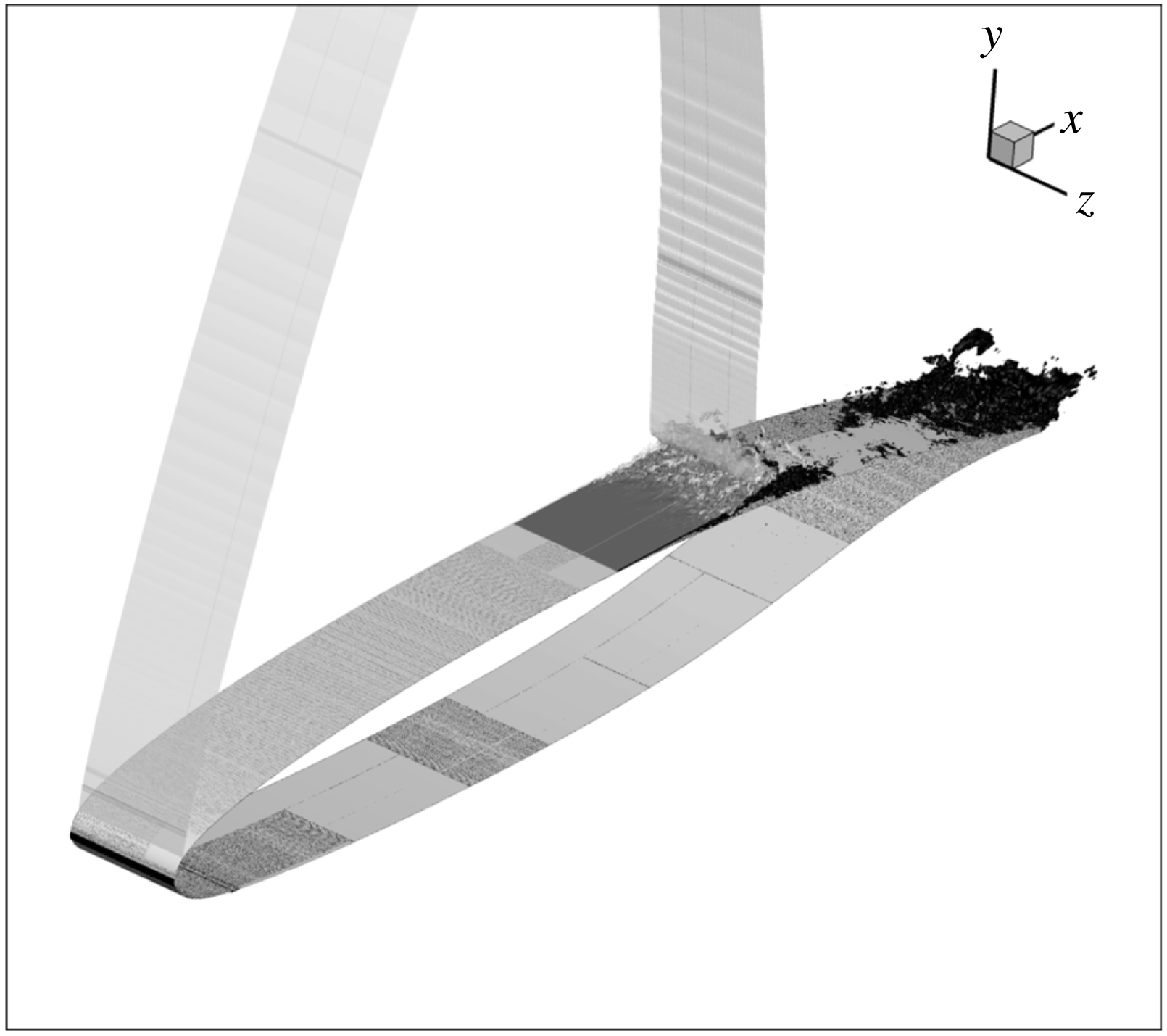
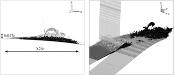
-criterion isosurface in figure 2, due to the turbulent structures, it is difficult to see if the flow is fully separated between the shock foot and the trailing edge. So, an isosurface
 $U_{x}/U_{\infty }=-4\times 10^{-4}$
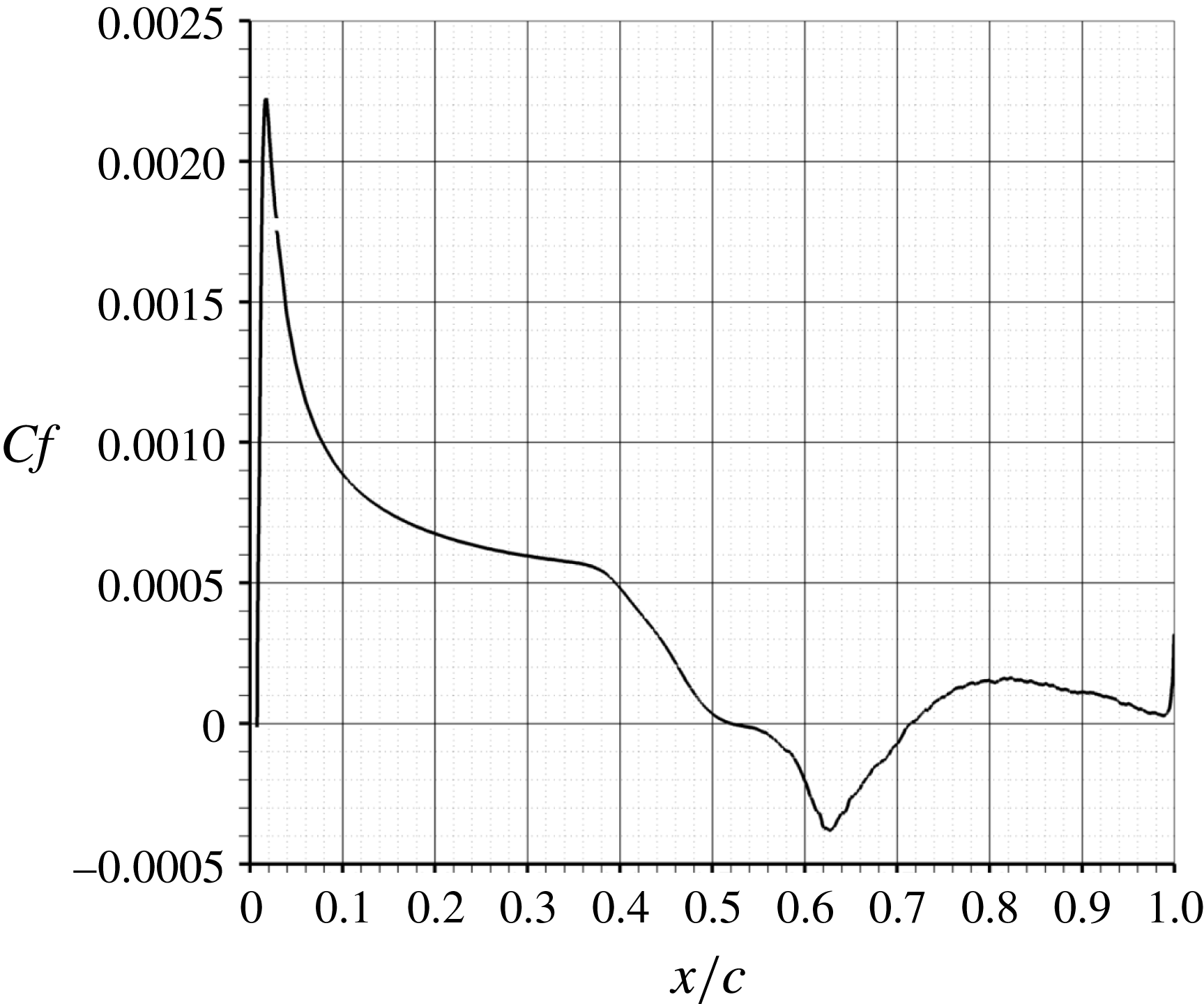
has been plotted in figures 4 and 5. One can see that in fact there are two separations: one at the shock foot and one at the trailing edge. Figure 5(a) shows that the separation bubble is very thin at the beginning and that it has a long streamwise extent of 26 % of chord. Downstream of this bubble, the flow reattaches and separates once again at the trailing edge over 10 % of chord. When looking at different time instants (see supplementary movie 1 available at https://doi.org/10.1017/jfm.2018.470), one can see that this second separation has been shed by the separation bubble at the shock foot. Vortices detach periodically from the bubble at the shock foot and are then convected towards the trailing edge. This will be explained in more detail in the phase-averaged flow analysis. On the time-averaged skin friction distribution (see figure 6), one can see that at the trailing edge, the flow is attached on average, which means that the separation between the shock foot and the trailing edge is intermittent.
Zoom on the
 $Q$
-criterion isosurface around the shock foot (a) and on the pressure side (b).

Isosurfaces
 $M=1$
and
 $U_{x}/U_{\infty }=-4\times 10^{-4}$
on an instantaneous field.

Zoom at the shock foot and at the trailing edge of the isosurfaces
 $M=1$
and
 $U_{x}/U_{\infty }=-4\times 10^{-4}$
on an instantaneous field.

4.2 Time-averaged data analysis
The streamwise evolution of the time-averaged skin friction coefficient is plotted in figure 6. The separation at the shock foot extends from
 $x/c=52$
to 71.4 % which means that the bubble length is equal to nearly 20 % of the chord length. The skin friction is minimum at the time-averaged shock location. The bubble thickness being equal to 0.43 % of the chord length, its aspect ratio is equal to 45.
Time-averaged skin friction coefficient distribution on the suction side.

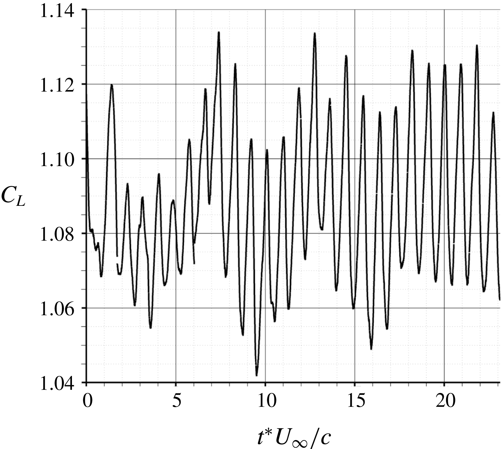
Figure 7 shows the time evolution of the lift coefficient. A well-marked period can be observed which corresponds to the shock oscillation at the laminar transonic buffet frequency. The time-averaged value is equal to 1.09.
Temporal evolution of the lift coefficient.

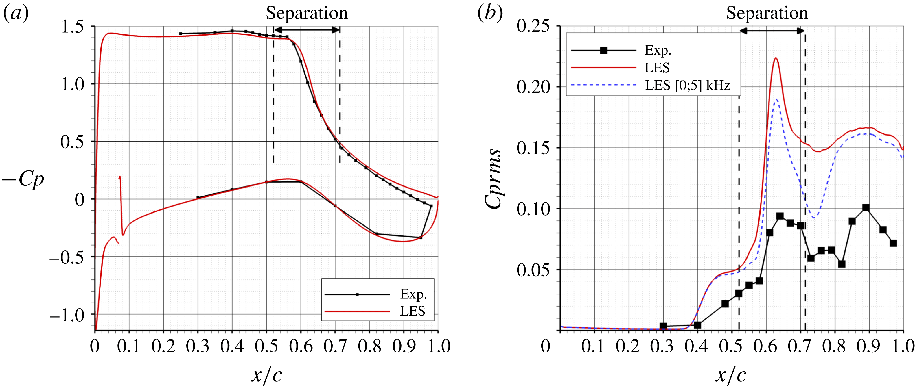
Figure 8 shows the chordwise evolution of the
 $Cp=(p-p_{0})/Q_{0}$
and
 $Cprms=p_{rms}/Q_{0}$
coefficients. There is a pressure plateau between
 $x/c=4$
and 43 % corresponding to the supersonic zone where
 $M\simeq 1.3$
. The small concavity between
 $x/c=43$
and 57 % is characteristic of the laminar separation bubble at the shock foot. The separation of the laminar boundary layer occurs at the middle of this concavity and the reattachment is downstream of the shock. The LES simulation predicts very well the length of the separation bubble at the shock foot and the shock location. The pressure at the trailing edge is slightly underestimated. On the lower side, the
 $Cp$
peak at
 $x/c=7\,\%$
corresponds to the boundary layer tripping.
Concerning the
 $Cprms$
distribution, the LES simulation curve (in red) has the same shape as the experimental one but overestimates the
 $Cprms$
level. There are two peaks: one at
 $x/c=63\,\%$
corresponding to the time-averaged shock location and one at
 $x/c=89\,\%$
corresponding to the travelling vortices (pressure minimum) from the shock foot towards the trailing edge. The overestimation of the
 $Cprms$
level can be partly explained by the fact that there remains a high level of energy in the pressure spectra for frequencies higher than one half of the experimental sampling frequency of 10 kHz. So, to realise a fair comparison with the numerical simulation, which has a frequency sampling of 1 MHz, the pressure spectra are integrated in the [0;5] kHz frequency band (blue dashed curve). The agreement with the experimental data on the
 $Cprms$
level is better. Another possible explanation is the small cavity between the hole on the model surface and the sensor which can act as a low-pass filter. It could explain why the
 $Cprms$
level is lower in the experiment than in the LES.
Time-averaged
 $Cp$
(a) and
 $Cprms$
(b) distributions.

4.3 Phase-averaged flow analysis
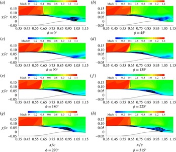
Figure 9 shows phase-averaged streamwise velocity fields. The initial phase has been chosen in order to have the shock at its most downstream location for
 $\unicode[STIX]{x1D719}=0^{\circ }$
. The vertical black line indicates the time-averaged shock location. A vortex is shed at the airfoil trailing edge between
 $\unicode[STIX]{x1D719}=45^{\circ }$
and
 $90^{\circ }$
. The separation at the shock foot reaches its maximum extension at
 $\unicode[STIX]{x1D719}=45^{\circ }$
. Then, at
 $\unicode[STIX]{x1D719}=90^{\circ }$
, the bubble bursts, a vortex is shed and starts travelling downstream. At
 $\unicode[STIX]{x1D719}=135^{\circ }$
, the flow is fully reattached at the shock foot. Then, a new cycle starts: a separation appears at
 $x/c=60\,\%$
for
 $\unicode[STIX]{x1D719}=180^{\circ }$
and grows up to
 $\unicode[STIX]{x1D719}=45^{\circ }$
. So, as one could expect, the bubble growth time is longer than the collapse time.
When looking at the shock oscillation, one can remark that this oscillation is mainly limited to
 $y/c<0.25$
. Above
 $y/c>0.4$
, the shock oscillation is not visible. This is a main difference with the turbulent transonic buffet, where the whole shock and not only its foot oscillates with a large amplitude of approximately 20 % of chord. In the laminar transonic buffet case, the shock oscillation is limited to a smaller area near the wall.
A maximum backflow velocity of
 $-0.23U_{ext}$
(where
 $U_{ext}$
is the streamwise velocity in the supersonic zone above the separation bubble) is found for
 $\unicode[STIX]{x1D719}$
between
 $270^{\circ }$
and
 $0^{\circ }$
just before the separation bubble reaches its maximum extension. On the time-averaged field, the maximum backflow velocity is equal
 $-0.09U_{ext}$
.
Phase-averaged Mach number field. The vertical black line indicates the time-averaged shock location.

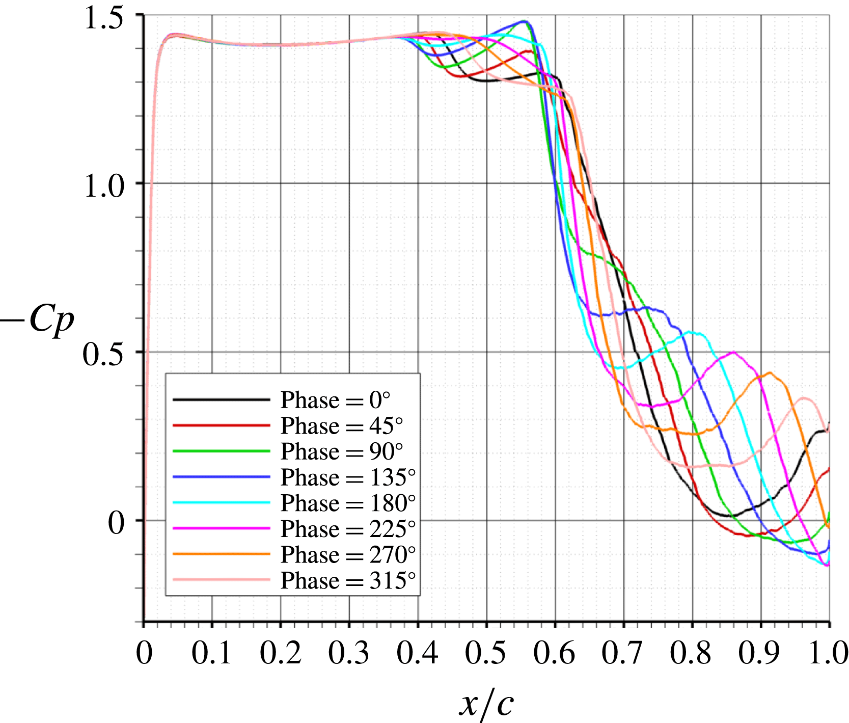
The phase-averaged wall pressure distributions are shown in figure 10. For
 $x/c<0.36$
, there is a pressure plateau, the flow is supersonic and is not influenced by the shock oscillation. Then, there is a first and small recompression between
 $x/c=0.4$
and 0.5, which is due to a compression wave originating at the separation point of the bubble and which is visible in figure 9(a–h). For example, in figure 9(a), at
 $x/c=0.44$
, which corresponds to the separation point, the Mach number decreases from
 $M=1.4$
to 1.3. The time-averaged value of this first recompression gives the concavity in the wall pressure distribution in figure 8 which is characteristic of the separation bubble at the shock foot. Between
 $x/c=0.6$
and 0.7, there is the second recompression which is due to the shock. The shock oscillation amplitude is equal to 6 % of chord. As explained in figure 9, this oscillation is limited to a small region around the shock foot and does not concern the whole shock as for the turbulent transonic buffet. More downstream, between
 $x/c=0.7$
and 1, there is
 $-Cp$
maximum (or pressure minimum) which is convected downstream and which corresponds to the flow acceleration above the vortex which has detached from the separation bubble at the shock foot. This flow acceleration above the vortex is clearly visible in figure 9. This
 $-Cp$
peak appears at
 $x/c=0.7$
for
 $\unicode[STIX]{x1D719}=90^{\circ }$
and reaches the trailing edge for
 $\unicode[STIX]{x1D719}=0^{\circ }$
. This means that the vortex has been convected on a length equal to 0.3 chord during three quarters of a period which gives an approximate convection velocity of
 $110~\text{m}~\text{s}^{-1}$
(or
 $U_{c}/U_{\infty }=0.45$
).
Phase-averaged
 $Cp$
distributions.

4.4 Signal processing
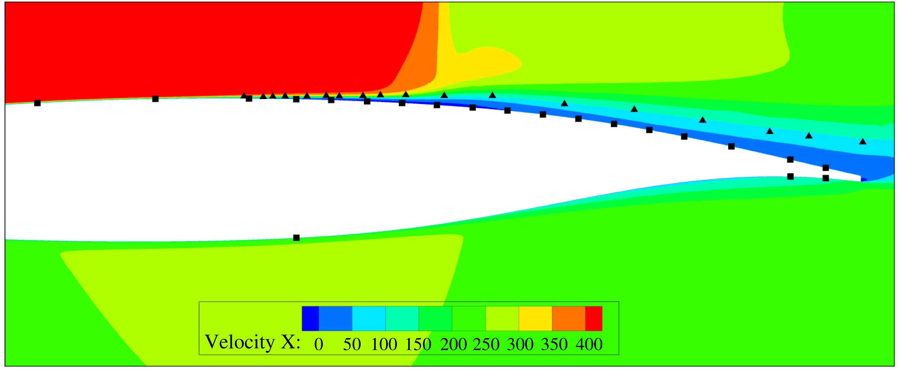
Figure 11 shows the locations of the unsteady pressure transducers on the wall model (black squares) and the additional numerical sensors in the fluid (black triangles). The numerical sensors follow the trajectory of the shear layer of the separation bubble and then the trajectory of the vortices shed downstream of the bubble towards the trailing edge.
For each sensor, the data have been collected on a duration equal to
 $100c/U_{\infty }$
, or 150 buffet periods. The frequency sampling is equal to 1 MHz or
 $935U_{\infty }/c$
. For all power spectral densities (PSDs) and cross-spectra presented below, Welch’s method with Hann windowing has been used with thirteen segments and 50 % overlap which results in a 59 Hz (
 $0.05U_{\infty }/c$
) resolution frequency.
Locations of the sensors (squares: experimental unsteady pressure transducers (wall surface), triangles: numerical sensors in the separated shear layer).

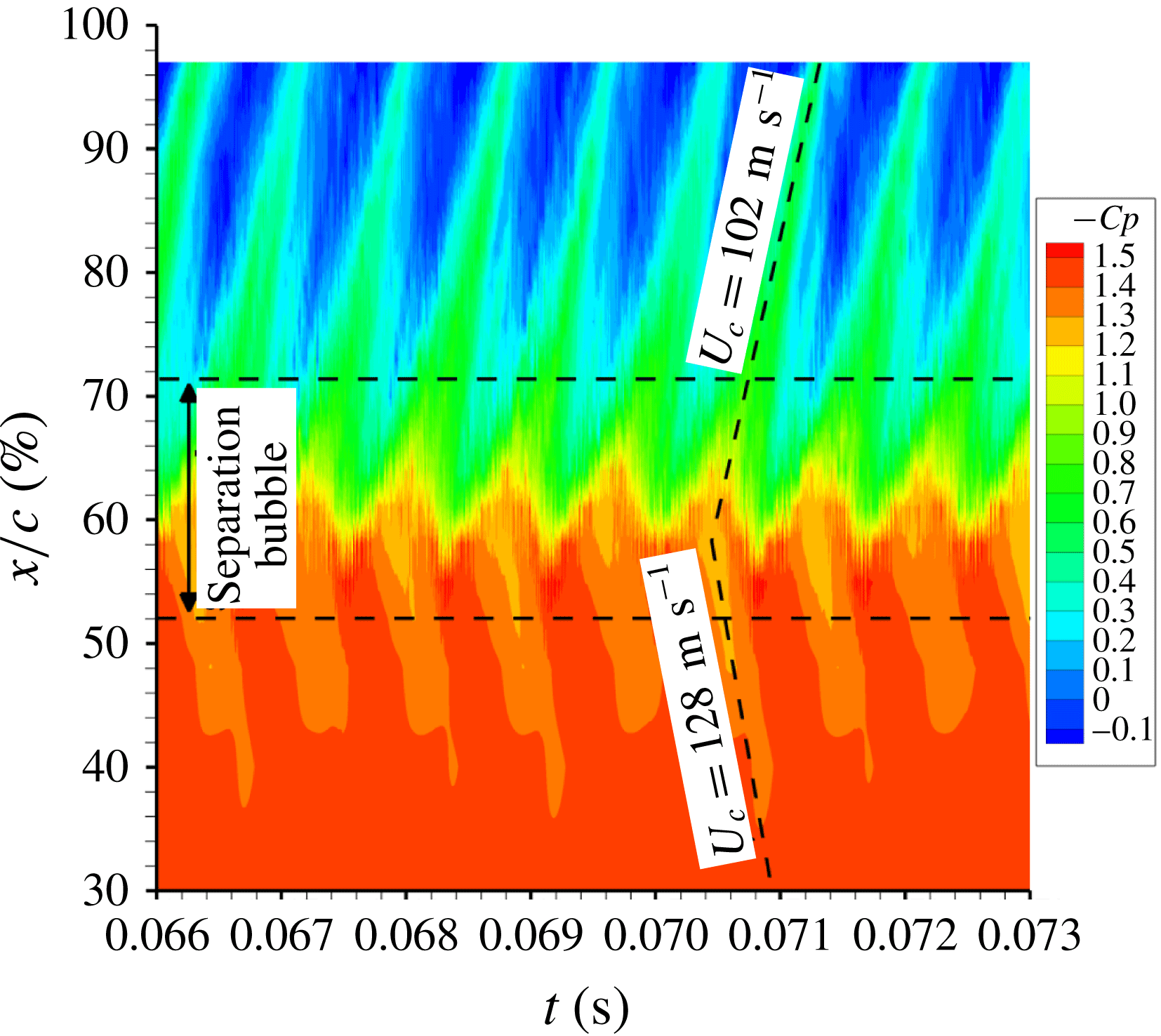
Figure 12 shows the wall pressure coefficient (on the suction side) as a function of time and streamwise coordinate. The separation bubble extent at the shock foot is marked by the two horizontal dashed lines. One can see the shock oscillation around
 $x/c=60\,\%$
. There are also lines of lower pressure (positive
 $Cp$
) from the shock foot up to the trailing edge. The period between these lines is very regular and corresponds to the laminar transonic buffet phenomenon. These lines are the footprint at the wall of the vortices which are shed by the separation bubble at the shock foot. These vortices are convected downstream at a velocity of approximately
 $102~\text{m}~\text{s}^{-1}$
(or
 $U_{c}/U_{\infty }=0.41$
). This value confirms that found by analysing figure 9.
Lines with a negative convection velocity can also been observed. During one phase of the buffet period, there is no longer a separation bubble at the shock foot. Then, a new bubble appears and there is a compression wave originating at its separation point. The footprint of this upstream movement of the bubble leads to a negative velocity of
 $-128~\text{m}~\text{s}^{-1}$
(or
 $U_{c}/U_{\infty }=-0.52$
). So, even if the flow is supersonic upstream of the shock, the information can move upstream in the boundary layer.
Wall pressure coefficient as function of time and streamwise coordinate for sensors at the wall.

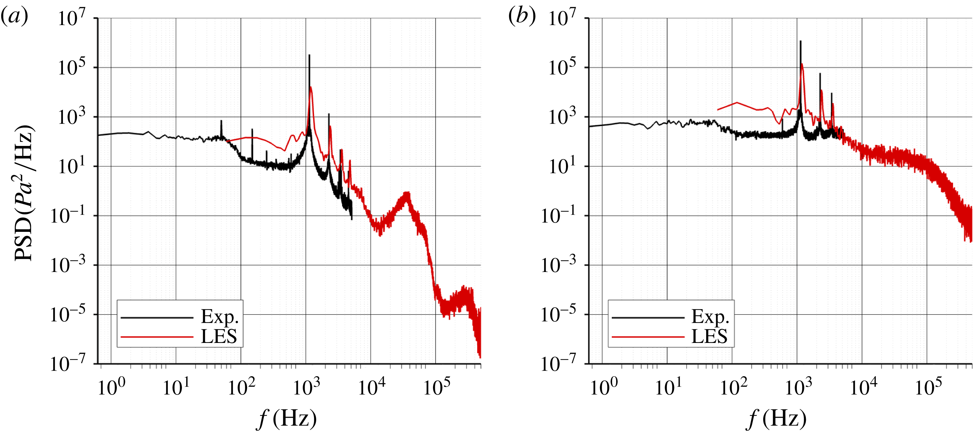
Figure 13 shows a comparison of the PSDs with the wind tunnel test for two sensors located at
 $x/c=52\,\%$
and 97 % on the suction side. The laminar transonic buffet frequency is very well predicted (1200 Hz in the LES (
 $St=1.12$
) compared to 1140 Hz (
 $St=1.06$
) in the experiment). Harmonics of the fundamental frequency are also clearly visible. At
 $x/c=52\,\%$
, which corresponds to the separation point of the bubble, a bump centred around 36 kHz (
 $St\simeq 34$
) is also visible and is due to the separated shear layer.
The theoretical Kelvin–Helmholtz (K–H) instability frequency is given by (see Huerre & Rossi Reference Huerre, Rossi, Godrèche and Manneville1998):
 $$\begin{eqnarray}f_{KH}(x)\simeq 0.135\frac{\overline{U}(x)}{\unicode[STIX]{x1D6FF}_{\unicode[STIX]{x1D714}}(x)},\end{eqnarray}$$
where
 $\overline{U}$
is the average of the velocity above (
 $u_{high}$
) and below (
 $u_{low}$
) the separated shear layer and
 $\unicode[STIX]{x1D6FF}_{\unicode[STIX]{x1D714}}$
is the vorticity thickness defined as:
 $$\begin{eqnarray}\unicode[STIX]{x1D6FF}_{\unicode[STIX]{x1D714}}(x)=\frac{u_{high}(x)-u_{low}(x)}{\max _{[y]}\displaystyle \left(\frac{\unicode[STIX]{x2202}u(x,y)}{\unicode[STIX]{x2202}y}\right)}.\end{eqnarray}$$
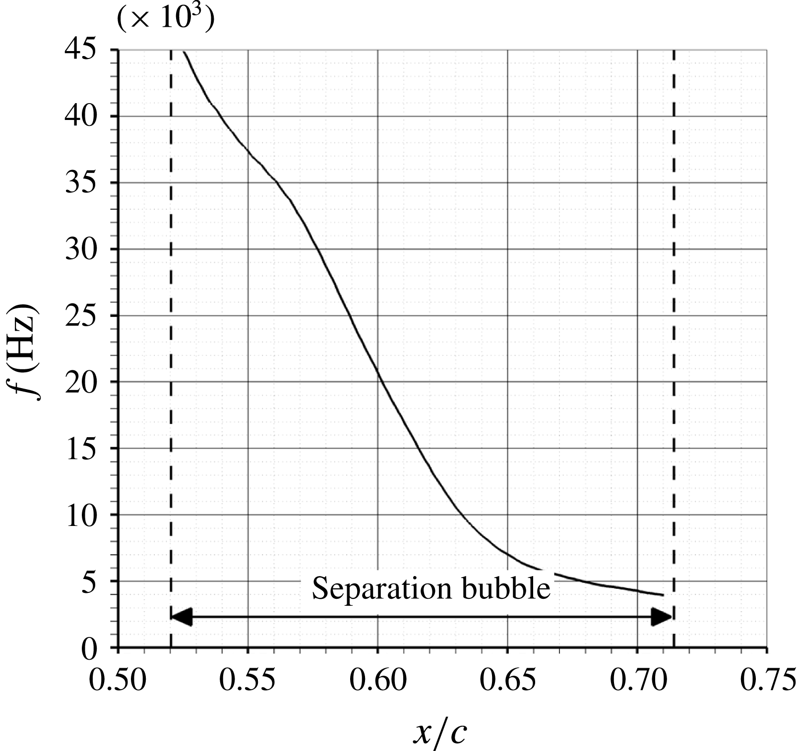
Figure 14 shows the streamwise evolution of the theoretical K–H frequency. At
 $x/c=52\,\%$
, the K–H frequency is around 45 kHz, which is close to the value found in the PSD at the same location taking into account the approximations on the determination of
 $u_{high}$
and
 $u_{low}$
. So, the frequency bump in figure 13 can be attributed to the K–H instability. The separation bubble is convectively unstable in its upstream part.
PSD at
 $x/c=52\,\%$
(a) and
 $x/c=97\,\%$
(b) (suction side).

Streamwise evolution of the estimated Kelvin–Helmholtz instability frequency.

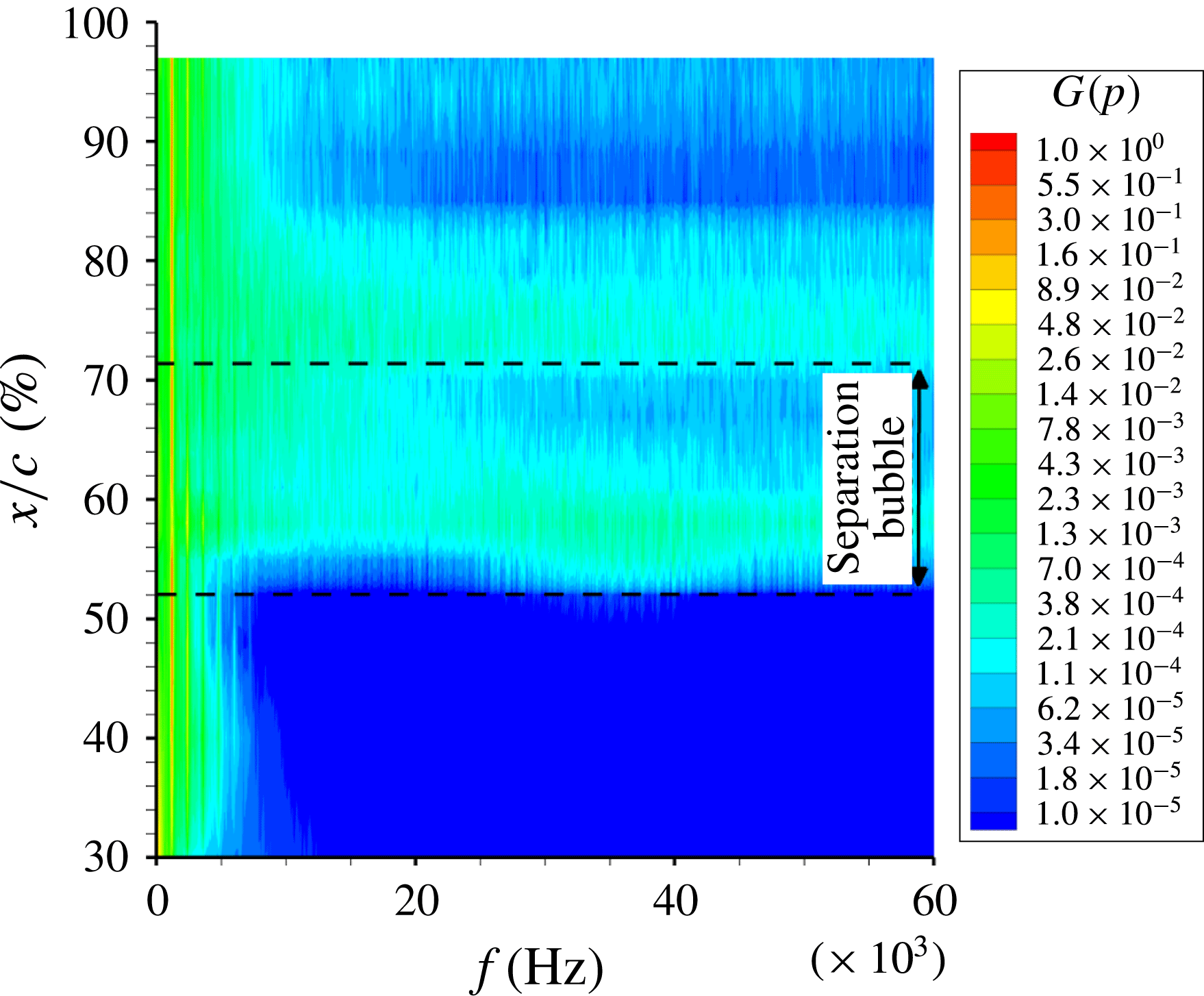
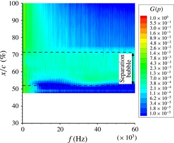
Figures 15 and 16 show contour maps of the PSDs at the wall and in the separated shear layer. For each sensor, the PSDs have been non-dimensionalised by the local value of the variance in order to highlight the high-frequency bump observed in figure 13 and to show the relative energy between each phenomenon (transonic buffet, K–H instability) at a given location. The laminar transonic buffet frequency is marked by vertical lines at 1.2 kHz, 2.4 kHz, etc. For the wall sensors, the high-frequency bump previously observed in figure 13 and corresponding to the K–H instability is visible at the separation and reattachment points whereas for the sensors in the separated shear layer, this bump is visible for all sensors between the separation and reattachment point.
PSD on the suction side at the wall.

PSD on the suction side in the separated shear layer.

Beneddine et al. (Reference Beneddine, Sipp, Arnault, Dandois and Lesshafft2016) have shown that the spatial structure of the spectral mode obtained by proper orthogonal decomposition filtering is very similar to the PSE (parabolised stability equations) field and also to the dominant optimal response mode of the resolvent at this frequency. To compute the spectral mode, the time series of vertical plane snapshots is divided into
 $N$
overlapping segments. For the present study,
 $N$
is equal to 11 with a 50 % overlap. For each segment, a fast Fourier transform (FFT) is performed. Then, instead of averaging the root-mean-square (r.m.s.) value of all the segments as in the classical Welch method, the complex fields from the FFT are used as snapshots to perform a proper orthogonal decomposition (POD) for each frequency. Since the first eigenvalue is two orders of magnitude larger than the second one, the POD filtering is obtained by only keeping the first POD mode. At the end, for each frequency, a complex velocity field is obtained and below only the real part of the mode is plotted. It is also possible to perform an animation by multiplying the complex field by
 $\text{e}^{\text{i}\unicode[STIX]{x1D714}t}$
and taking the real part. Figure 17 shows contour maps of the normalised spectral mode of the streamwise velocity obtained by POD filtering for the buffet frequency (
 $St=1.12$
, a) and for the Kelvin–Helmholtz instability frequency (
 $St\simeq 34$
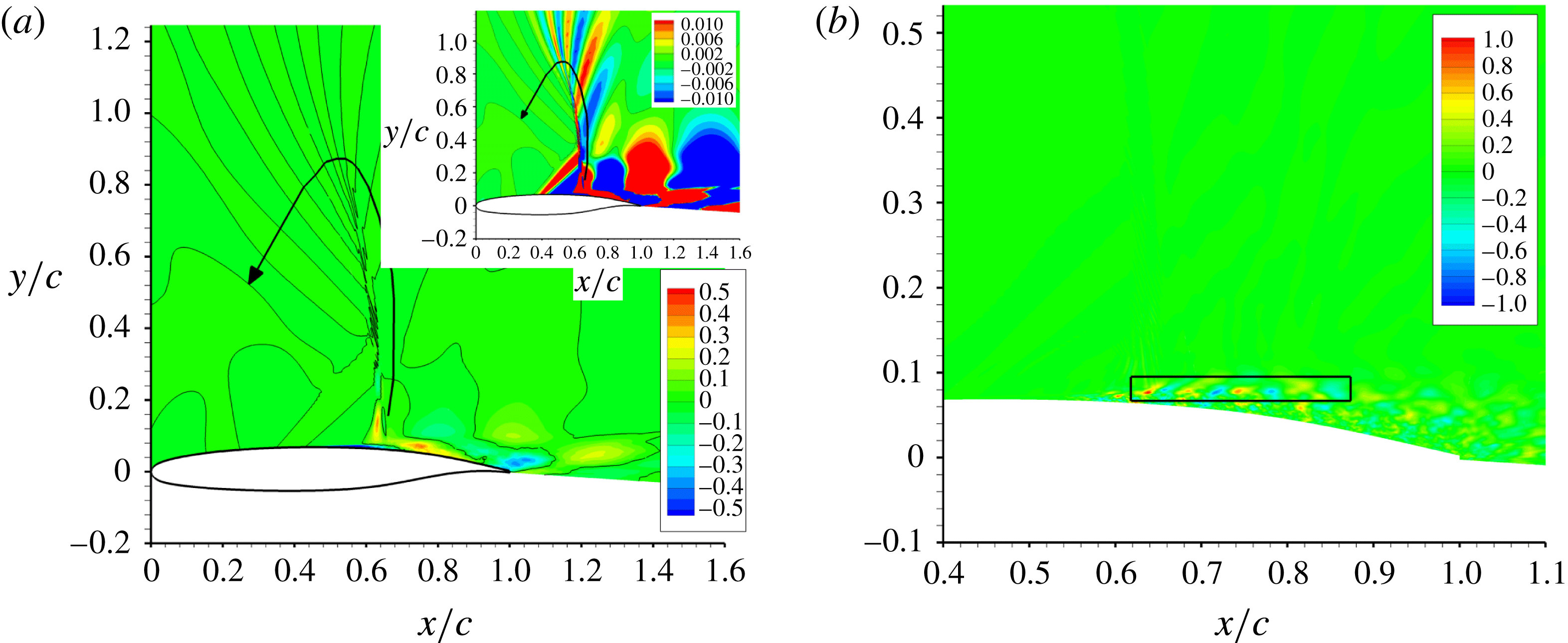
, b). Concerning the buffet frequency, the dark lines corresponds to a value equal to zero. Alternating signs of the streamwise velocity fluctuation are found between the shock and the wake corresponding to the convection of the vortices shed from the separation bubble at the shock foot. Alternating values are also found vertically at the shock location which correspond to the shock oscillation (upper right figure with a different scale). It shows that the shock oscillation is coupled with the vortex shedding phenomenon. As shown by the black arrow, an animation of the dark lines corresponding to a value equal to zero shows that the velocity perturbations propagate also vertically downstream of the shock (see supplementary movie 2). Then, they travel upstream above the shock and towards the wall. Concerning the K–H instability, alternating values of the streamwise velocity fluctuation are found in the shear layer of the separation bubble and correspond to the convection of spanwise rollers.
Contour maps of the normalised spectral mode of the streamwise velocity obtained by POD filtering for the buffet frequency (
 $St=1.12$
, a) and for the Kelvin–Helmholtz instability frequency (
 $St\simeq 34$
, b).

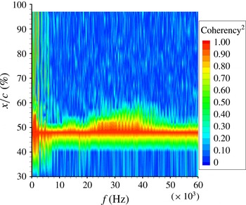
Cross-spectra between all sensors at the wall has then been computed. Figure 18 shows the coherency. The coherency is defined as:
 $$\begin{eqnarray}\unicode[STIX]{x1D6FE}_{xy}^{2}(f)=\frac{|S_{xy}(f)|^{2}}{S_{xx}(f)S_{yy}(f)},\end{eqnarray}$$
where
 $S_{xx}$
and
 $S_{yy}$
are the PSDs of
 $x(t)$
and
 $y(t)$
and
 $S_{xy}$
is the cross-spectral density of the signals defined as:
 $$\begin{eqnarray}S_{xy}(f)=\int _{-\infty }^{\infty }R_{xy}(t)\text{e}^{-j\unicode[STIX]{x1D714}t}\,\text{d}t=\int _{-\infty }^{\infty }\left[\int _{-\infty }^{\infty }x(\unicode[STIX]{x1D70F})y(\unicode[STIX]{x1D70F}+t)\,\text{d}\unicode[STIX]{x1D70F}\right]\text{e}^{-j\unicode[STIX]{x1D714}t}\,\text{d}t,\end{eqnarray}$$
where
 $R_{xy}$
is the cross-correlation of
 $x(t)$
and
 $y(t)$
. The reference sensor has been put at
 $x/c=48\,\%$
which is the reason why the coherency is equal to one at this location. Vertical lines of high coherency values at frequencies corresponding to the laminar transonic buffet phenomenon and its harmonics (1.2 kHz, 2.4 kHz, etc.) can be observed. Between 20 kHz and 50 kHz, there is bump of high coherency values which is limited to locations in the separation bubble.
Coherency between sensors on the suction side at the wall.

To compute the convection velocities of each phenomenon, the phase of the cross-spectra has been also analysed. It is defined as:
 $$\begin{eqnarray}\unicode[STIX]{x1D6F7}_{xy}(f)=\arctan \left(\frac{\text{Im}[S_{xy}(f)]}{\text{Re}[S_{xy}(f)]}\right).\end{eqnarray}$$
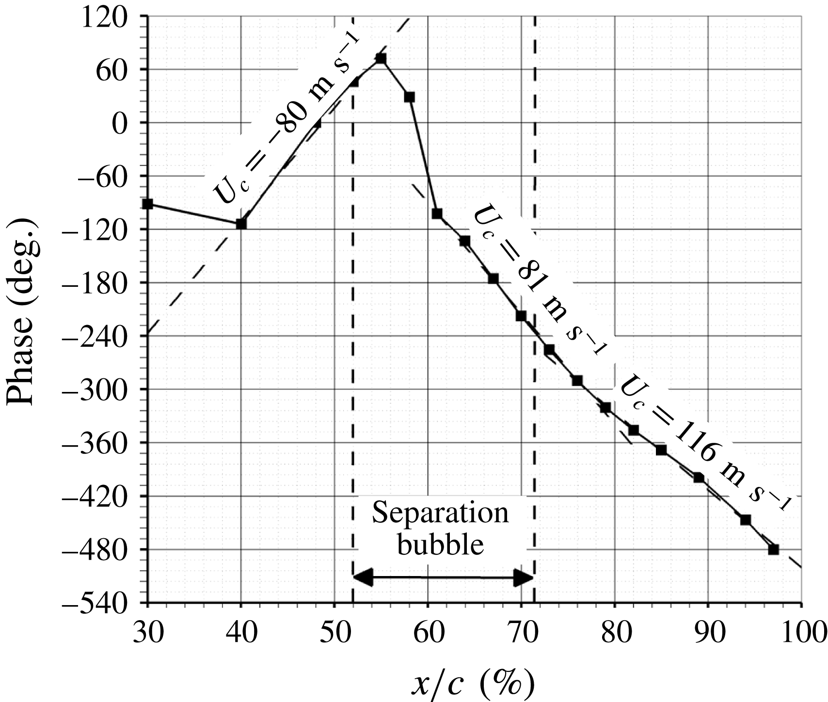
This signal processing tool is more precise than the pressure evolution in figure 12 since it is based on averaged data at a precise frequency which can be chosen to select one phenomenon (transonic buffet or K–H instability). Figure 19 shows the phase evolution with
 $x/c$
at the laminar transonic buffet frequency (1.2 kHz,
 $St=1.12$
) between sensors at the wall. Regions of linear evolution correspond to constant convection velocities. Upstream of the time-averaged shock location, a negative convection velocity equal to
 $-80~\text{m}~\text{s}^{-1}$
(or
 $U_{c}/U_{\infty }=-0.32$
) is found. This velocity has been attributed in figure 12 to the upstream movement of the separation point. The extent of this negative convection velocity zone from 40 to 55 % of chord corresponds very well to the oscillation area of the separation point found in the phase-averaged fields in figure 9.
Downstream of the time-averaged shock location, two convection velocities of
 $81~\text{m}~\text{s}^{-1}$
(or
 $U_{c}/U_{\infty }=0.33$
) and
 $116~\text{m}~\text{s}^{-1}$
(or
 $U_{c}/U_{\infty }=0.47$
) are found. If this convection velocities are non-dimensionalised by the external flow velocity downstream of the shock (
 $U_{ext}\simeq 260~\text{m}~\text{s}^{-1}$
), the two convection velocities are
 $U_{c}/U_{ext}=0.31$
and 0.45. These velocities correspond to the convection velocity of the vortex shed from the separation bubble at the shock foot. Non-dimensionalised values around 0.5 are generally found in the literature for the convection of the vortex shedding phenomenon (see table 3 from Dandois, Garnier & Sagaut (Reference Dandois, Garnier and Sagaut2007)).
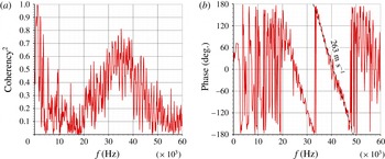
Figure 20 shows the coherency and the phase between sensors at
 $x/c=48\,\%$
and 55 % as a function of the frequency. The coherency is high at the buffet frequency as well as in the frequency band [20;50] kHz. In this frequency band, regions of constant slope correspond to a convection phenomenon. Here, this is the case between 20 and 50 kHz, so for frequencies corresponding to the K–H instability. A convection velocity of
 $263~\text{m}~\text{s}^{-1}$
(or
 $U_{c}/U_{\infty }=0.6$
) is found which is in good agreement with the values found for this phenomenon in the literature (Dandois et al.
Reference Dandois, Garnier and Sagaut2007).
Phase evolution with
 $x/c$
at the laminar transonic buffet frequency between sensors on the suction side at the wall.

Coherency (a) and phase (b) between sensors at
 $x/c=48$
and 55 % on the suction side at the wall.

5 Discussion
As recalled in the introduction, the turbulent transonic buffet phenomenon is characterised by a well-marked peak in the power spectra at a low frequency (see Jacquin et al. Reference Jacquin, Molton, Deck, Maury and Soulevant2009). In the wind tunnel tests of Brion et al. (Reference Brion, Dandois, Abart and Paillart2017), with a different airfoil geometry than in Jacquin et al. (Reference Jacquin, Molton, Deck, Maury and Soulevant2009) (OALT25 instead of OAT15A) but for the same airfoil chord and the same flow conditions, the same buffet frequency is observed which shows that the turbulent transonic buffet frequency is not very sensitive to the airfoil geometry but mainly to the chord length and flow conditions (the transonic buffet frequency increases with the angle of attack and slightly with the Mach number, see Crouch et al. Reference Crouch, Garbaruk, Magidov, Jacquin, Braza and Hourigan2009a ).
On the same airfoil without boundary layer tripping, the flow is laminar up to the shock foot where the transition occurs in the separation bubble. The present LES results exhibit also well marked peaks in the wall pressure spectra but at a much higher frequency than the turbulent transonic buffet (
 $St=1.1$
instead of 0.07 so 17 times higher) for a nearly identical free-stream Mach number (
 $M=0.735$
instead of 0.73) and the same Reynolds number. The shock oscillation amplitude is also much lower than in the turbulent case (6 % of chord instead of 20 %) which seems logical since the frequency is higher. Moreover, this oscillation is limited to the shock foot area contrary to the turbulent transonic buffet.
One first question which arises is: what can explain this order of magnitude difference between the turbulent and the laminar transonic buffet frequency?
What is observed experimentally is that the laminar transonic buffet frequency decreases when the Mach number or the angle of attack increases. It decreases from
 $St=1.18$
at
 $M=0.72$
to
 $St=0.83$
at
 $M=0.78$
. Of course, there is also a Reynolds number variation but it is much more limited: from
 $Re_{c}=2.79\times 10^{6}$
at
 $M=0.72$
to
 $Re_{c}=2.91\times 10^{6}$
at
 $M=0.78$
. This is in opposition to the turbulent transonic buffet phenomenon for which the frequency increases with the Mach number or the angle of attack (see Crouch et al.
Reference Crouch, Garbaruk, Magidov, Jacquin, Braza and Hourigan2009a
). In the laminar regime, one natural explanation of this frequency decrease is that the higher the Mach number, the stronger the shock-wave boundary layer interaction which leads to a larger and thicker separation bubble. So, possible candidates for a characteristic length are the separation bubble length or its height. The Strouhal number based on the time-averaged separation bubble length and the local (not free stream) flow velocity is
 $St_{L}=0.13$
and based on its height
 $St_{h}=0.0029$
. Based on the displacement thickness at the separation point
 $\unicode[STIX]{x1D6FF}^{\ast }=5.5\times 10^{-4}~\text{m}$
, the Strouhal number
 $St_{\unicode[STIX]{x1D6FF}}^{\ast }$
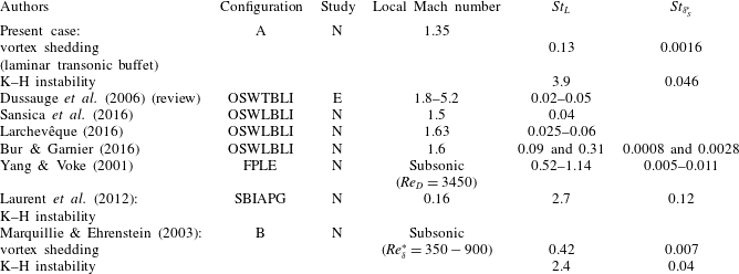
is equal to 0.0016. Compared to the literature on oblique (and not normal as in the present case) SWBLI (see table 1), the vortex shedding (or laminar transonic buffet) Strouhal number is slightly higher but of the same order of magnitude (0.13 against 0.02–0.09 depending of the studies). As pointed out in the introduction, the physical mechanism is the same: the low-frequency unsteadiness of the SWBLI is due to a bubble breathing with vortices shed downstream but in one case the shock is oblique and in the present case, it is normal. Concerning the K–H instability in the separated shear layer, the Strouhal number found in the present case is of the same order of magnitude as that found in the literature.
Vortex shedding and Kelvin–Helmholtz instability frequencies for different flows (configuration type: A
 $=$
airfoil, OSWTBLI
 $=$
oblique shock-wave turbulent boundary layer interaction, OSWLBLI
 $=$
oblique shock-wave laminar boundary layer interaction, FPLE
 $=$
flat plate leading edge, SBIAPG
 $=$
separation bubble induced by an adverse pressure gradient, B
 $=$
bump; study type: E
 $=$
experimental study, N
 $=$
numerical study).

An important question is whether the laminar separation bubble presents an absolute instability or not. As explained in the introduction, it has been demonstrated by Crouch et al. (Reference Crouch, Garbaruk, Magidov and Travin2009b ) and Sartor et al. (Reference Sartor, Mettot and Sipp2014) that the turbulent transonic buffet phenomenon is due to a global instability. The question is then: is the laminar transonic buffet phenomenon also due to a global instability?
When looking at the wall pressure spectra, there is a well-marked peak (and not a large bump) as in the turbulent transonic buffet phenomenon for which we already know that there is a global instability (Crouch et al. Reference Crouch, Garbaruk, Magidov and Travin2009b ). So, the fact that the laminar transonic buffet is characterised by a peak rather than a bump tends to support the hypothesis that there is also a global instability of the separation bubble at the shock foot. So, like in Marquillie & Ehrenstein (Reference Marquillie and Ehrenstein2003) and using their non-dimensionalisation by the displacement thickness at the separation point, the present flow would exhibit two instabilities:
(i) a convective one: the K–H instability at
 $St_{L}=3.9$
or
$St_{\unicode[STIX]{x1D6FF}}^{\ast }=0.046$
;
(ii) and an absolute one: the bubble vortex shedding which is the cause of the laminar transonic buffet at
$St_{L}=0.13$
or
$St_{\unicode[STIX]{x1D6FF}}^{\ast }=0.0016$
.


Huerre & Rossi (Reference Huerre, Rossi, Hussaini, Kumar and Streett1991), Hammond & Redekopp (Reference Hammond and Redekopp1998), Alam & Sandham (Reference Alam and Sandham2000) and Rist (Reference Rist2004) have studied the conditions for the presence of an absolute instability. The conclusion is that at large Reynolds numbers (
 $Re_{\unicode[STIX]{x1D6FF}}^{\ast }>2000$
, based on the displacement thickness
 $\unicode[STIX]{x1D6FF}^{\ast }$
), the flows are absolutely unstable for reverse flows in excess of 15 %. Here,
 $Re_{\unicode[STIX]{x1D6FF}^{\ast }}=6750$
so the backflow velocity to have an absolute instability is equal to 15 %. As explained in § 4.3, the time-averaged maximum backflow velocity is equal
 $-0.09U_{ext}$
so there should not be an absolute instability and consequently not a global instability. Nevertheless, during some part of the oscillation cycle, between
 $\unicode[STIX]{x1D719}=270^{\circ }$
and
 $0^{\circ }$
just before the separation bubble reaches its maximum extension, a maximum backflow velocity of
 $-0.23U_{ext}$
is observed, so larger than the required backflow velocity to be absolutely unstable. As for the turbulent transonic buffet, it would be necessary to perform a global stability analysis to definitively conclude on this point.
6 Conclusion
The present paper has presented for the first time results from a large-eddy simulation of laminar transonic buffet on an airfoil at
 $M=0.735$
,
 $\unicode[STIX]{x1D6FC}=4^{\circ }$
,
 $Re_{c}=3\times 10^{6}$
. The objective was to improve the knowledge on the laminar transonic buffet phenomenon. First, the analysis of instantaneous flow fields has shown that the boundary layer was laminar up to the shock foot and laminar/turbulent transition occurs in the separation bubble at the shock foot. On the pressure side, the boundary layer was tripped at
 $x/c=7\,\%$
as in the wind tunnel tests.
The analysis of the time-averaged wall pressure distribution has evidenced the presence of a small concavity between
 $x/c=43$
and 57 % which is characteristic of a separation bubble at the shock foot. The separation extends from
 $x/c=52$
to 71.4 % which means that the bubble length is equal to nearly 20 % of the chord length. The bubble thickness is equal to 0.43 % of chord length so the aspect ratio is equal to 45.
The analysis of the phase-averaged flow fields has shown that shock oscillation amplitude was smaller than in the turbulent regime: 6 % and limited to the shock foot area in the laminar case instead of 20 % with a whole shock oscillation and intermittent boundary layer separation and reattachment in the turbulent case. Moreover, the analysis of the phase-averaged fields allowed linking of the laminar transonic buffet frequency to a separation bubble breathing phenomenon with vortices which are shed from the shock foot towards the trailing edge. These vortices are convected at
 $U_{c}/U_{\infty }\simeq 0.4$
.
The wall pressure spectra are characterised by well-marked peaks as in the turbulent regime but at a much higher frequency (
 $St=f\cdot c/U_{\infty }=1.2$
instead of
 $St\simeq 0.06{-}0.07$
). In addition to the laminar transonic buffet frequency, the Kelvin–Helmholtz instability occurs in the shear layer between the separation bubble and the external flow. The frequency as well as the convection velocity (
 $U_{c}/U_{\infty }=0.6$
) agree well the literature.
The main finding of the present paper is that the higher frequency of the shock oscillation in the laminar regime is due to a different mechanism than in the turbulent one: laminar transonic buffet is due to a separation bubble breathing phenomenon occurring at the shock foot whereas turbulent transonic buffet is due to a global instability of the flow with intermittent boundary layer separation and reattachment between the shock and the trailing edge.
The analysis of the time-averaged backflow velocity (9 % of
 $U_{ext}$
) has shown that, given the Reynolds number
 $Re_{\unicode[STIX]{x1D6FF}^{\ast }}$
, it is lower than the required velocity (15 %) to have an absolute instability. Nevertheless, during some phases of the shock oscillation, the maximum backflow velocity is equal to 23 %. Further work is needed to definitely conclude whether the laminar transonic buffet phenomenon is due a global instability of the separation bubble at the shock foot or not.
Acknowledgement
This work has been supported by the European FP7 Project BUTERFLI (FP7-AAT-2013.8-1-RTDRUSSIA) program.
Supplementary movies
Supplementary movies are available at https://doi.org/10.1017/jfm.2018.470.