1 Introduction
Ludwig Prandtl’s slope flow model permits an exact solution to the Navier–Stokes equations, including heat transfer at an infinitely wide inclined surface immersed within a stably stratified medium (Prandtl Reference Prandtl1942). The model has been found to describe qualitatively the vertical profiles of wind speed and temperature associated with katabatic winds in mountainous terrain or over large ice sheets in Antarctica and the Arctic or Greenland (Fedorovich & Shapiro Reference Fedorovich and Shapiro2009). The validity of certain simplifying assumptions in Prandtl’s model, such as perfect horizontal spatial homogeneity or constant fluid viscosity, have been questioned (Grisogono & Oerlemans Reference Grisogono and Oerlemans2001a,Reference Grisogono and Oerlemansb), and it has been found that adopting a gradually varying eddy viscosity improves the fit between model predictions and experimental field data.
In addition to Prandtl’s original formulation, which assumes local equilibrium, bulk-averaged models of increasing sophistication have been developed and applied by Fleagle (Reference Fleagle1950), Manins & Sawford (Reference Manins and Sawford1979a,Reference Manins and Sawfordb), Kondo & Sato (Reference Kondo and Sato1988), Fitzjarrald (Reference Fitzjarrald1984) and Ellison & Turner (Reference Ellison and Turner1959) to predict the along-slope progression of the katabatic boundary layers. Fitzjarrald (Reference Fitzjarrald1984) extended this model by accounting for the presence of opposing ambient flow which counteracts the katabatic wind, which is also discussed in Zardi & Whiteman (Reference Zardi and Whiteman2013). Laboratory experiments were performed by Ellison & Turner (Reference Ellison and Turner1959) to empirically determine the flow entrainment rate as a function of the local Richardson number of flow velocity. The drawback of these bulk models is that information about the vertical flow profile is sacrificed in favour of resolving along-slope variation of bulk-averaged quantities, which may obscure subtle dynamics that can trigger flow instabilities and lead to transition to turbulence. In that regard, Prandtl’s model can be seen as an antipode to these models, since it aims at describing the vertical structure of katabatic winds instead of their along-slope variation, which is zero under the assumption of an infinite slope.
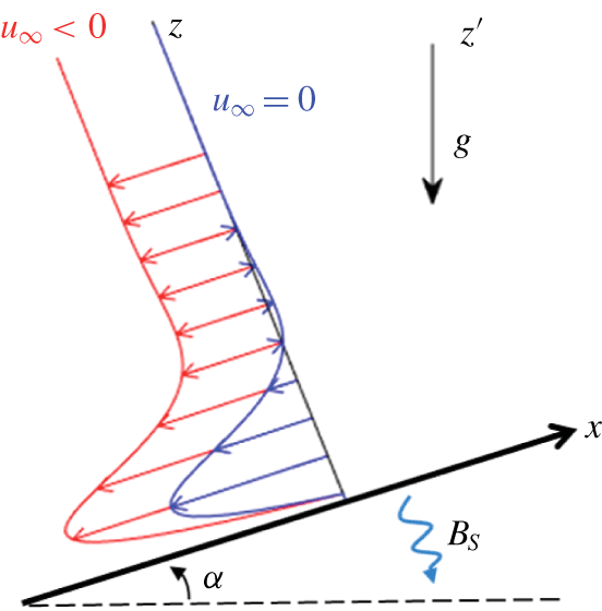
Prandtl assumed quiescent winds at high altitudes in his slope model. It is also common in mountain meteorology for katabatic winds to develop in the presence of an external ambient wind field aloft, as for example when stably stratified air flows over a long mountain range, resulting in a non-zero wind in the free stream (Manins & Sawford Reference Manins and Sawford1979a; Whiteman Reference Whiteman2000; Whiteman & Zhong Reference Whiteman and Zhong2008). The presence of ambient wind has been known to make it more difficult to fit observed field data into predictions of simple katabatic flow models (Doran & Horst Reference Doran and Horst1983; Doran, Horst & Whiteman Reference Doran, Horst and Whiteman1990; Haiden & Whiteman Reference Haiden and Whiteman2005). Lykosov & Gutman (Reference Lykosov and Gutman1972) incorporated the effect of a uniform ambient wind field into Prandtl’s original formulation. We will henceforth refer to their model as the extended Prandtl model. Katabatic wind profiles above an inclined cooled slope depicted by the original and the extended Prandtl model are shown in figure 1. The vertical profiles of buoyancy and velocity as predicted by the original Prandtl model are exponentially damped sinusoidal solutions. In the original Prandtl model, the near-surface jet along the slope descent is capped by a weak reverse flow. The extended Prandtl model appears as a mere shifting of the velocity profile produced by the original Prandtl model. However, as the equations indicate, the downslope ambient wind also increases the velocity maximum of the near-surface jet. This extended model can be accepted as a valid approximation to a situation in which stably stratified air flows over the top of an elevated terrain and follows the underlying surface closely (Whiteman Reference Whiteman2000). In the present work, we adopt the extended Prandtl model with the assumption that the ambient wind is directed downslope without cross-slope components and remains parallel to the inclined plane underneath.
In Xiao & Senocak (Reference Xiao and Senocak2019), we investigated the linear stability of the katabatic flows under the original Prandtl model and uncovered transverse and longitudinal modes of flow instabilities that emerge as a function of the slope angle, Prandtl number and a new dimensionless number, which we have designated the stratification perturbation parameter. This new dimensionless number represents the importance of heat exchange at the surface relative to the strength of the ambient stratification, and it is defined solely by the intrinsic parameters of the flow problem at hand, and thus physically more insightful for the problem at hand than the more familiar internal Froude or Richardson numbers. However, by using ‘derived’ internal length and velocity scales in the original Prandtl model,  $\unicode[STIX]{x1D6F1}_{s}$ can be converted to a bulk Richardson or internal Froude number, creating a misleading interpretation that there is no necessity for a new dimensionless parameter. In the present work, we demonstrate that
 $\unicode[STIX]{x1D6F1}_{s}$ intrinsically exists alongside another new dimensionless number and, for fixed Prandtl number, these two dimensionless numbers along with the inclination angle describe the dynamic stability of stably stratified slope flows under the combined action of ambient wind and surface cooling. Here, we pursue the same technical approach and methods outlined in Xiao & Senocak (Reference Xiao and Senocak2019) to determine the stability limits of the extended Prandtl model to comprehend the effect of a uniform ambient wind field on the stability katabatic slope flows.
Velocity profiles corresponding to the extended (red) and the original Prandtl model (blue) for slope flows. A rotated coordinate system is adopted.

2 Governing equations
Let us consider the slope flow under the action of an ambient wind as depicted in figure 1, where  $\unicode[STIX]{x1D6FC}$ is the slope angle and
 $B_{S}$ is the constant negative heat flux imposed at the surface. The constant ambient wind speed in the free stream is
 $U_{\infty }$. For ease of analysis, the problem is studied in a rotated Cartesian coordinate system whose
 $x$ axis is aligned with the planar inclined surface and points along the upslope direction.
Let  $b$ be the scalar buoyancy variable, and
 $u$ the along-slope (longitudinal),
 $v$ the cross-slope (transverse) and
 $w$ the slope-normal velocity components, such that
 $u_{i}=[u,v,w]$ is the velocity vector, where a positive value of
 $u$ is associated with the upslope direction.
 $g_{i}=[g_{1},g_{2},g_{3}]=[\sin \unicode[STIX]{x1D6FC},0,\cos \unicode[STIX]{x1D6FC}]$ are the components of the non-dimensional gravity vector, and we will also refer the spatial coordinate components
 $(x_{j})$ in the rotated frame as
 $(x,y,z)$. The ambient wind vector is assumed to be of the form
 $(U_{j})=(U_{\infty },0,0),U_{\infty }<0$. The governing equations for conservation of momentum and energy under the Boussinesq approximation for an incompressible flow can be written as follows:
 $$\begin{eqnarray}\displaystyle & \displaystyle \frac{\unicode[STIX]{x2202}u_{i}}{\unicode[STIX]{x2202}t}+\frac{\unicode[STIX]{x2202}u_{i}u_{j}}{\unicode[STIX]{x2202}x_{j}}=-\frac{1}{\unicode[STIX]{x1D70C}}\frac{\unicode[STIX]{x2202}p}{\unicode[STIX]{x2202}x_{i}}+\frac{\unicode[STIX]{x2202}}{\unicode[STIX]{x2202}x_{j}}\left(\unicode[STIX]{x1D708}\frac{\unicode[STIX]{x2202}u_{i}}{\unicode[STIX]{x2202}x_{j}}\right)+bg_{i}, & \displaystyle\end{eqnarray}$$
 $$\begin{eqnarray}\displaystyle & \displaystyle \frac{\unicode[STIX]{x2202}b}{\unicode[STIX]{x2202}t}+\frac{\unicode[STIX]{x2202}bu_{j}}{\unicode[STIX]{x2202}x_{j}}=\frac{\unicode[STIX]{x2202}}{\unicode[STIX]{x2202}x_{j}}\left(\unicode[STIX]{x1D6FD}\frac{\unicode[STIX]{x2202}b}{\unicode[STIX]{x2202}x_{j}}\right)-N^{2}g_{j}(u_{j}-U_{j}), & \displaystyle\end{eqnarray}$$
where  $\unicode[STIX]{x1D708}$ is the kinematic viscosity and
 $\unicode[STIX]{x1D6FD}$ is the thermal diffusivity.
 $N=\!\sqrt{(g/\unicode[STIX]{x1D6E9}_{r})(\unicode[STIX]{x2202}\unicode[STIX]{x1D6E9}_{e}/\unicode[STIX]{x2202}z^{\prime })}$ is the Brunt–Väisälä frequency, assumed to be constant,
 $\unicode[STIX]{x1D6E9}$ is the potential temperature, and
 $z^{\prime }$ is the vertical coordinate in the non-rotated coordinate system. Buoyancy is related to the potential temperature
 $\unicode[STIX]{x1D6E9}$ as
 $b=g(\unicode[STIX]{x1D6E9}-\unicode[STIX]{x1D6E9}_{e})/\unicode[STIX]{x1D6E9}_{r}$, where
 $\unicode[STIX]{x1D6E9}_{r}$ is a reference potential temperature and
 $\unicode[STIX]{x1D6E9}_{e}$ is the environmental potential temperature. The governing equations are completed by the divergence-free velocity field condition for incompressible flows.
Following the same assumptions as in the original Prandtl model, equations (2.1)–(2.2) reduce to simple momentum and buoyancy balance equations. Lykosov & Gutman (Reference Lykosov and Gutman1972) presented an exact solution for the case with constant temperature at the surface and ambient wind parallel to the surface. Here, we follow the approach presented in Shapiro & Fedorovich (Reference Shapiro and Fedorovich2004) and modify that solution for constant surface buoyancy flux at the surface. The modified solution takes the following form:
 $$\begin{eqnarray}\displaystyle & \displaystyle u=\left[\left(U_{\infty }+\sqrt{2}u_{0}\right)\sin \left(z_{n}/\sqrt{2}\right)-U_{\infty }\cos \left(z_{n}/\sqrt{2}\right)\right]\exp \left(-z_{n}/\sqrt{2}\right)+U_{\infty }, & \displaystyle\end{eqnarray}$$
 $$\begin{eqnarray}\displaystyle & \displaystyle b=\frac{2\unicode[STIX]{x1D708}}{z_{0}^{2}\sin \unicode[STIX]{x1D6FC}}\left[\left(U_{\infty }+\sqrt{2}u_{0}\right)\cos \left(z_{n}/\sqrt{2}\right)+U_{\infty }\sin \left(z_{n}/\sqrt{2}\right)\right]\exp \left(-z_{n}/\sqrt{2}\right)\!,\quad & \displaystyle\end{eqnarray}$$
where  $z_{n}=z/l_{0}$ is the non-dimensional height. Fedorovich & Shapiro (Reference Fedorovich and Shapiro2009) have proposed the following flow scales for the original Prandtl model, which we use for the present flow problem as well:
 $$\begin{eqnarray}\displaystyle & l_{0}=(\unicode[STIX]{x1D708}\unicode[STIX]{x1D6FD})^{1/4}N^{-1/2}\sin ^{-1/2}\unicode[STIX]{x1D6FC}, & \displaystyle\end{eqnarray}$$
 $$\begin{eqnarray}\displaystyle & u_{0}=(\unicode[STIX]{x1D708}\unicode[STIX]{x1D6FD})^{-1/4}N^{-3/2}B_{s}\sin ^{-1/2}\unicode[STIX]{x1D6FC}, & \displaystyle\end{eqnarray}$$
 $$\begin{eqnarray}\displaystyle & \displaystyle b_{0}=\left.\frac{\unicode[STIX]{x2202}b}{\unicode[STIX]{x2202}z}\right|_{0}\cdot l_{0}=\frac{B_{s}}{\unicode[STIX]{x1D6FD}}l_{0}, & \displaystyle\end{eqnarray}$$
where  $Pr\equiv \unicode[STIX]{x1D708}/\unicode[STIX]{x1D6FD}$ is the Prandtl number. As an extension to the velocity scale defined above, we introduce a composite velocity scale
 $U_{c}$ as the sum of the inner velocity scale
 $u_{0}$ and the outer velocity scale
 $U_{\infty }$, which is the ambient wind in this case, as follows:
 $$\begin{eqnarray}U_{c}=u_{0}+U_{\infty }.\end{eqnarray}$$
It can be shown via calculus that for all values of  $u_{0},U_{\infty }<0$, the normalised maximal velocity
 $\hat{u} _{max}=u_{max}/U_{c}$ of the flow profile as well as normalised location
 $\hat{z}_{max}=z_{max}/l_{0}$ where this maximum is attained always lie within a constant, finite interval; to be more specific, we have
 $\hat{z}_{max}\in [\unicode[STIX]{x03C0}/4,\unicode[STIX]{x03C0}/2]$, and the normalised maximal velocity at
 $\hat{z}_{max}$ lies within
 $[0.45,1.21]$. Thus the choice of the velocity scale
 $u_{c}$ and length scale
 $l_{0}$ is both simple and meaningful for this class of flow profiles.
We observe from (2.3) that the velocity profile exhibits the expected near-surface jet and approaches the ambient wind speed  $U_{\infty }$ at higher altitudes. This trend implies the existence of two distinct velocity scales, one that is associated with the processes near the surface based on the near-surface jet, and another one that represents the ambient wind aloft. Thus, no matter which velocity scale is chosen, the flow profiles in the extended Prandtl model cannot be normalised to a universal form independent of the wind speed
 $U_{\infty }$, in contrast to the original Prandtl model with
 $U_{\infty }=0$.
Let us now consider the Buckingham- $\unicode[STIX]{x03C0}$ theorem to determine the dimensionless numbers involved in the extended Prandtl model for slope flows. One can show that any non-dimensional dependent variable (for example, non-dimensional maximum jet velocity) is a function of the following four independent dimensionless parameters:
 $$\begin{eqnarray}\displaystyle \unicode[STIX]{x1D6FC},\quad Pr\equiv \frac{\unicode[STIX]{x1D708}}{\unicode[STIX]{x1D6FD}},\quad \unicode[STIX]{x1D6F1}_{s}\equiv \frac{|B_{s}|}{\unicode[STIX]{x1D6FD}N^{2}},\quad \unicode[STIX]{x1D6F1}_{w}\equiv \frac{U_{\infty }^{2}}{\unicode[STIX]{x1D708}N}. & & \displaystyle\end{eqnarray}$$
Due to the lack of an externally imposed length scale, familiar dimensionless numbers such as the Reynolds, Richardson, or Froude number do not appear in the above list, and all the dimensionless numbers are functions of the externally imposed dimensional parameters in the slope flow problem only.
The new dimensionless number in the above set is  $\unicode[STIX]{x1D6F1}_{w}$. It is interesting to observe that
 $\unicode[STIX]{x1D6F1}_{w}$ can be expressed as the product of the Reynolds and internal Froude numbers:
 $$\begin{eqnarray}\displaystyle \unicode[STIX]{x1D6F1}_{w}=Re\cdot Fr=\frac{U_{\infty }L}{\unicode[STIX]{x1D708}}\cdot \frac{U_{\infty }}{LN}. & & \displaystyle\end{eqnarray}$$
We note that both the  $Re$ number and the
 $Fr$ number requires the specification of an external characteristic length scale
 $L$. From (2.10), we also observe that the external length scale
 $L$ cancels out, further supporting our argument that an external length scale is absent in the extended Prandtl slope flow model. Our statement, however, does not imply the non-existence of a length scale in the flow problem. The flow will eventually exhibit a length scale as quantified by (2.5). However, this length scale should be viewed as a ‘internal’ quantity as opposed to a characteristic external scale that is imposed on the flow problem.
In Xiao & Senocak (Reference Xiao and Senocak2019),  $\unicode[STIX]{x1D6F1}_{s}$ was introduced as the stratification perturbation number. Here, we designate
 $\unicode[STIX]{x1D6F1}_{w}$ the wind forcing number, and interpret it as the ratio of the kinetic energy in the ambient wind to the damping of kinetic energy in the flow due to the action of viscosity and the stabilising effect of stratification, which is also supported by the expression given in (2.10).
3 Linear stability analysis
We introduce the normalised velocity and buoyancy as  $u_{n}=u/u_{c},b_{n}=b/b_{0}$, and use
 $l_{0}$ to normalise all lengths. Linearising around the base flow given by (2.3)–(2.4), and assuming that disturbances are waves of the form
 $\boldsymbol{q}(x,y,z,t)=\hat{\boldsymbol{q}}(z)\exp \{\text{i}(k_{x}x+k_{y}y)+\unicode[STIX]{x1D714}t\}$, the resulting equations have the form
 $$\begin{eqnarray}\displaystyle & \displaystyle \text{i}k_{x}\hat{u} +\text{i}k_{y}\hat{v}+\frac{\unicode[STIX]{x2202}{\hat{w}}}{\unicode[STIX]{x2202}z}=0, & \displaystyle\end{eqnarray}$$
 $$\begin{eqnarray}\displaystyle & \displaystyle \unicode[STIX]{x1D714}\hat{u} +\text{i}u_{n}k_{x}\hat{u} +u_{n}^{\prime }{\hat{w}}=-\text{i}k_{x}\hat{p}-\frac{Pr\,\sin \unicode[STIX]{x1D6FC}}{C}\left(-(k_{x}^{2}+k_{y}^{2})\hat{u} +\frac{\unicode[STIX]{x2202}^{2}\hat{u} }{\unicode[STIX]{x2202}z^{2}}\right)-\frac{\unicode[STIX]{x1D6F1}_{s}Pr\,\sin \unicode[STIX]{x1D6FC}}{C^{2}}\hat{b},\qquad & \displaystyle\end{eqnarray}$$
 $$\begin{eqnarray}\displaystyle & \displaystyle \unicode[STIX]{x1D714}\hat{v}+\text{i}u_{n}k_{x}\hat{v}=-\text{i}k_{y}\hat{p}-\frac{Pr\,\sin \unicode[STIX]{x1D6FC}}{C}\left(-(k_{x}^{2}+k_{y}^{2})\hat{v}+\frac{\unicode[STIX]{x2202}^{2}\hat{v}}{\unicode[STIX]{x2202}z^{2}}\right), & \displaystyle\end{eqnarray}$$
 $$\begin{eqnarray}\displaystyle & \displaystyle \unicode[STIX]{x1D714}{\hat{w}}+\text{i}u_{n}k_{x}{\hat{w}}=-\frac{\unicode[STIX]{x2202}\hat{p}}{\unicode[STIX]{x2202}z}-\frac{Pr\,\sin \unicode[STIX]{x1D6FC}}{C}\left(-(k_{x}^{2}+k_{y}^{2}){\hat{w}}+\frac{\unicode[STIX]{x2202}^{2}{\hat{w}}}{\unicode[STIX]{x2202}z^{2}}\right)-\frac{\unicode[STIX]{x1D6F1}_{s}Pr\cos \unicode[STIX]{x1D6FC}}{C^{2}}\hat{b}, & \displaystyle\end{eqnarray}$$
 $$\begin{eqnarray}\displaystyle & \displaystyle \unicode[STIX]{x1D714}\hat{b}+\text{i}u_{n}k_{x}\hat{b}+b_{n}^{\prime }{\hat{w}}=-\frac{\sin \unicode[STIX]{x1D6FC}}{C}\left(-(k_{x}^{2}+k_{y}^{2})\hat{b}+\frac{\unicode[STIX]{x2202}^{2}\hat{b}}{\unicode[STIX]{x2202}z^{2}}\right)+\frac{1}{\unicode[STIX]{x1D6F1}_{s}}(\hat{u} \sin \unicode[STIX]{x1D6FC}+{\hat{w}}\cos \unicode[STIX]{x1D6FC}),\qquad & \displaystyle\end{eqnarray}$$
where i is the imaginary unit, and  $\hat{u} ,\hat{v},{\hat{w}},\hat{p},\hat{b}$ are flow disturbances varying along the slope-normal direction normalised by
 $u_{c},b_{0}$, respectively. Here
 $z$ is the distance to the slope surface normalised by the length scale
 $l_{0}$; and
 $k_{x},k_{y}$ are normalised positive wavenumbers in the
 $x$ (along-slope) and
 $y$ (transverse) directions, respectively, whereas
 $\unicode[STIX]{x1D714}$ is a normalised complex frequency. The normalised base flow solution and its derivative in the slope-normal direction in normalised coordinates are denoted by
 $u_{n},b_{n}$ and
 $u_{n}^{\prime },b_{n}^{\prime }$, respectively. The coefficient
 $C=\unicode[STIX]{x1D6F1}_{s}+\sqrt{\unicode[STIX]{x1D6F1}_{w}}Pr^{3/4}\sin ^{1/2}\unicode[STIX]{x1D6FC}$ is introduced solely for convenience, and we choose
 $\unicode[STIX]{x1D6F1}_{w}$ instead of
 $\sqrt{\unicode[STIX]{x1D6F1}_{w}}Pr^{3/4}\sin ^{1/2}\unicode[STIX]{x1D6FC}$ as the dimensionless parameter such that it is independent of the slope angle
 $\unicode[STIX]{x1D6FC}$ and Prandtl number
 $Pr$, which are separate dimensionless numbers of the configuration.
The solution method for the above generalised eigenvalue problem follows the same approach as described in Xiao & Senocak (Reference Xiao and Senocak2019). The stability behaviour of the problem is encoded by the eigenvalues  $\unicode[STIX]{x1D714}$, whose real part equals the exponential growth rate and whose imaginary part is the temporal oscillation frequency of the corresponding eigenmode.
3.1 Dependence of instability modes on dimensionless parameters
From the results in Xiao & Senocak (Reference Xiao and Senocak2019), it is known that without ambient winds, the dominant instability of Prandtl’s profile for katabatic flows at each angle is either a stationary transverse mode, i.e. varying purely along the cross-slope direction, or a longitudinal mode travelling along-slope. This means that the instability growth rate as a function of the wavenumber vectors  $(k_{x},k_{y})$ attains its maximum only when one of the wavenumbers
 $k_{x},k_{y}$ is zero. It turns out that the same also holds true for katabatic flows in the presence of ambient winds; hence the growth rate contours for disturbances in the wave vector space, looking qualitatively similar to those in Xiao & Senocak (Reference Xiao and Senocak2019), will not be shown here.
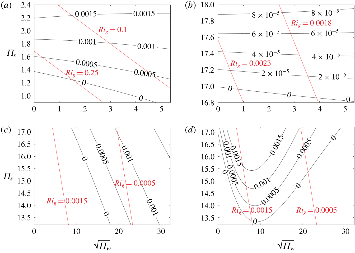
Contours of maximal growth rates at  $\unicode[STIX]{x1D6FC}=4^{\circ }$ for (a) transverse and (b) longitudinal modes depending on wind forcing number
 $\unicode[STIX]{x1D6F1}_{w}$ and stratification perturbation
 $\unicode[STIX]{x1D6F1}_{s}$. The same contours at
 $\unicode[STIX]{x1D6FC}=67^{\circ }$ for (c) transverse and (d) longitudinal modes. Red lines are contours of the gradient Richardson number calculated from (3.6).

The fact that the most dominant instability is either a pure transverse ( $k_{x}=0$) or longitudinal mode (
 $k_{y}=0$) means that at a fixed configuration, determined by the slope angle
 $\unicode[STIX]{x1D6FC}$ and the parameters
 $\unicode[STIX]{x1D6F1}_{s},\unicode[STIX]{x1D6F1}_{w}$, the most dominant instability can be found by searching for one of the wavenumbers
 $k_{x}$ or
 $k_{y}$ which maximises the growth rate, setting the other wavenumber to zero. This approach has been applied to obtain the growth rate contour of the strongest transverse and longitudinal modes over the
 $\unicode[STIX]{x1D6F1}_{w},\unicode[STIX]{x1D6F1}_{s}$ space for different slope angles, as shown in figure 2. At each given angle
 $\unicode[STIX]{x1D6FC}$ and ambient wind value specified by
 $\unicode[STIX]{x1D6F1}_{w}$, the most dominant amongst the transverse and longitudinal modes is identified as the one which attains critical stability (zero growth rate) at a smaller
 $\unicode[STIX]{x1D6F1}_{s}$ value. We would like to remark that for typical values of
 $N,\unicode[STIX]{x1D708},Pr,B_{s},U_{\infty }$ found in nocturnal atmospheric conditions (Fedorovich, Gibbs & Shapiro Reference Fedorovich, Gibbs and Shapiro2017), the dimensionless parameters
 $\unicode[STIX]{x1D6F1}_{s},\unicode[STIX]{x1D6F1}_{w}$ would be on the order of
 $10^{6}$ and
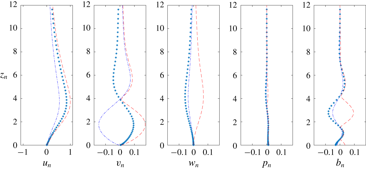
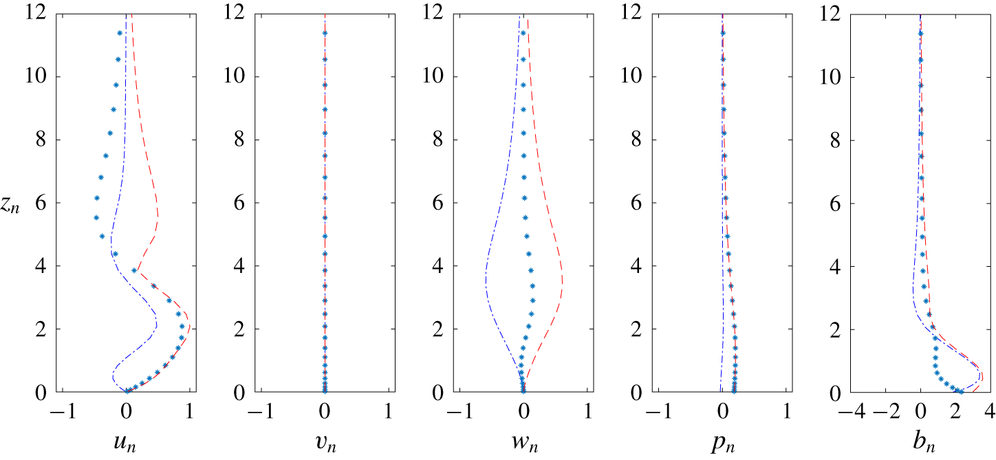
 $10^{9}$, respectively; thus many orders of magnitude higher than the threshold value required to trigger the instabilities. The vertical profile of the eigenfunctions corresponding to disturbances of each instability mode are shown in figures 3 and 4, from which it can be seen that the transverse mode at
 $4^{\circ }$ is three-dimensional, whereas the longitudinal mode at
 $67^{\circ }$ has no cross-slope velocity component and is hence two-dimensional.
Since the gradient Richardson number  $Ri_{g}$ features prominently in the study of stratified flows, we also overlay the corresponding
 $Ri_{g}$ number on the contour plots in figure 2. The
 $Ri_{g}$ number used in those figures is calculated from the extended Prandtl model velocity profile (2.3) and reduces to the following convenient formula with the help of the dimensionless parameters
 $\unicode[STIX]{x1D6F1}_{s},\unicode[STIX]{x1D6F1}_{w}$ defined in (2.9):
 $$\begin{eqnarray}Ri_{g}=\frac{N^{2}}{\left({\displaystyle \frac{\unicode[STIX]{x2202}u}{\unicode[STIX]{x2202}z}}\right)_{max}^{2}}=\frac{Pr}{\left(\sqrt{2\unicode[STIX]{x1D6F1}_{w}}Pr^{3/4}\sin ^{1/2}\unicode[STIX]{x1D6FC}+\unicode[STIX]{x1D6F1}_{s}\right)^{2}},\end{eqnarray}$$
where it can be shown that the maximum shear is attained at the slope surface. We can observe that  $Ri_{g}$ number decreases with an increase of either of the parameters
 $\unicode[STIX]{x1D6F1}_{s}$ or
 $\unicode[STIX]{x1D6F1}_{w}$. However, since
 $Ri_{g}$ is a function depending on three independent variables
 $\unicode[STIX]{x1D6FC},\unicode[STIX]{x1D6F1}_{s},\unicode[STIX]{x1D6F1}_{w}$ for a fixed
 $Pr$ number, it is possible from (3.6) to find different combinations of their values which lead to the same
 $Ri_{g}$ number. By inspecting the normalised partial derivative
 $(\unicode[STIX]{x2202}Ri_{g}/\unicode[STIX]{x2202}\unicode[STIX]{x1D6FC})/Ri_{g}$, it can be concluded that for fixed
 $\unicode[STIX]{x1D6F1}_{s},\unicode[STIX]{x1D6F1}_{w}\gg 1$,
 $Ri_{g}$ becomes insensitive to variations of slope angle
 $\unicode[STIX]{x1D6FC}$. This means that at those more unstable flow configurations, the
 $Ri_{g}$ number remains almost constant for all angles
 $\unicode[STIX]{x1D6FC}$.
Eigenfunctions of the dominant instability at  $\unicode[STIX]{x1D6F1}_{s}=1.2,\unicode[STIX]{x1D6F1}_{w}=20$ (stationary transverse mode) at
 $\unicode[STIX]{x1D6FC}=4^{\circ }$. Dash-dotted lines represent the real part, asterisks represent the imaginary part, and dashed line is the magnitude. The disturbance magnitudes have been normalised with the maximal occurring along-slope velocity disturbance magnitude in each case.

Eigenfunctions of the dominant instability at  $\unicode[STIX]{x1D6F1}_{s}=17,\unicode[STIX]{x1D6F1}_{w}=20$ (propagating longitudinal mode) at
 $\unicode[STIX]{x1D6FC}=67^{\circ }$. Dash-dotted lines represent the real part, asterisks represent the imaginary part, and dashed line is the magnitude. The disturbance magnitudes have been normalised with the maximal occurring along-slope velocity disturbance magnitude in each case.

We note that Richardson number contours, calculated using (3.6), appear as straight lines on the  $\sqrt{\unicode[STIX]{x1D6F1}_{w}}-\unicode[STIX]{x1D6F1}_{s}$ plane. Thus, figure 2 and subsequent plots adopt
 $\sqrt{\unicode[STIX]{x1D6F1}_{w}}$ instead of
 $\unicode[STIX]{x1D6F1}_{w}$ as the horizontal axis. But as the results shown in figure 2 demonstrate, different values for either of these dimensionless parameters can have profoundly different effects on the linear stability of the underlying base flow. For example, at different slope angles, the dominant instability may change from either the stationary transverse mode or the travelling longitudinal mode to the other instability, respectively. From the plots shown in figure 2, we observe that increasing the ambient wind tends to lower an instability’s growth rate at the same
 $Ri_{g}$ number, i.e. the most unstable mode at fixed
 $Ri_{g}$ is found at
 $U_{\infty }=0$, which is the original Prandtl model as analysed in Xiao & Senocak (Reference Xiao and Senocak2019). At the low slope angle of
 $\unicode[STIX]{x1D6FC}=4^{\circ }$, it can be observed that for the wind forcing number
 $\unicode[STIX]{x1D6F1}_{w}<3$, the base flow can be unstable despite possessing a larger
 $Ri_{g}$ number than the critical value
 $Ri_{g}=0.25$. This counterexample to the celebrated Miles–Howard stability theorem has already been shown in Xiao & Senocak (Reference Xiao and Senocak2019) for the Prandtl base flow without ambient wind, and has been attributed to the presence of surface inclination, heat transfer at the surface, and viscosity.
We observe from figure 2 that an increase of surface buoyancy, as measured by the dimensionless number  $\unicode[STIX]{x1D6F1}_{s}$, is a monotonically destabilising effect for both the transverse and longitudinal modes. This finding is in agreement with the stability results for the original Prandtl model as demonstrated in Xiao & Senocak (Reference Xiao and Senocak2019). However, we would like to remark that the purely destabilising effect of negative surface buoyancy flux applies only under the ideal conditions assumed by the Prandtl model, where a larger magnitude of the buoyancy flux increases the near-surface jet velocity (2.6), which leads to an increase of maximum shear and thus lowers the gradient Richardson number (3.6). The effect of
 $\unicode[STIX]{x1D6F1}_{w}$ on the instabilities, however, is slightly more complex. Figures 2(a) and 2(c) indicate that for both slope angles
 $\unicode[STIX]{x1D6FC}=4^{\circ },67^{\circ }$, the growth rate of the most unstable transverse mode grows monotonically with an increase in
 $\unicode[STIX]{x1D6F1}_{w}$. As shown in Xiao & Senocak (Reference Xiao and Senocak2019), at low slope angles devoid of an external ambient wind forcing (i.e.
 $U_{\infty }=0$), the transverse mode is the dominant instability. Thus, at those angles, when all other flow parameters are left unchanged, ambient wind has a strictly destabilising effect on the base flow field. This behaviour is consistent with expectations, since increasing the ambient wind also increases the maximal shear of the base flow profile given in (2.4), thus decreasing the
 $Ri_{g}$ number, according to (3.6).
For the longitudinal instability mode at the steep angle of  $\unicode[STIX]{x1D6FC}=67^{\circ }$, however, an increase
 $\unicode[STIX]{x1D6F1}_{w}$ only destabilises the mode when
 $\unicode[STIX]{x1D6F1}_{w}\leqslant 100$; beyond the approximate value
 $\unicode[STIX]{x1D6F1}_{w}\approx 100$, increasing
 $\unicode[STIX]{x1D6F1}_{w}$ starts to decrease the mode’s growth rate, thus stabilising the mode, which runs counter to expectations. Since the longitudinal mode is the dominant instability at steep angles in the absence of ambient wind, when the surface buoyancy measured by
 $\unicode[STIX]{x1D6F1}_{s}$ is kept constant, increasing the ambient wind from the value corresponding to
 $\unicode[STIX]{x1D6F1}_{w}=100$ onwards tends to stabilise the flow. As is known from (3.6), the
 $Ri_{g}$ number is monotonically decreasing with respect to
 $\unicode[STIX]{x1D6F1}_{w}$, so this behaviour implies that a lowering of
 $Ri_{g}$ stabilises the base flow, which is an unexpected finding. However, since it is known that the ambient wind is monotonically destabilising for the transverse mode, this effect can only persist until the ambient wind becomes large enough such that the growth rate of the previously dormant transverse mode overtakes that of its longitudinal counterpart, thus becoming the dominant instability. Such a complex behaviour of the stability region due to both stabilising as well as destabilising effects of an external flow parameter has also been discovered in Schörner, Reck & Aksel (Reference Schörner, Reck and Aksel2016), who reported the simultaneous stabilising as well as destabilising effects of topography on gravity-driven viscous film flows beyond the Nusselt regime.
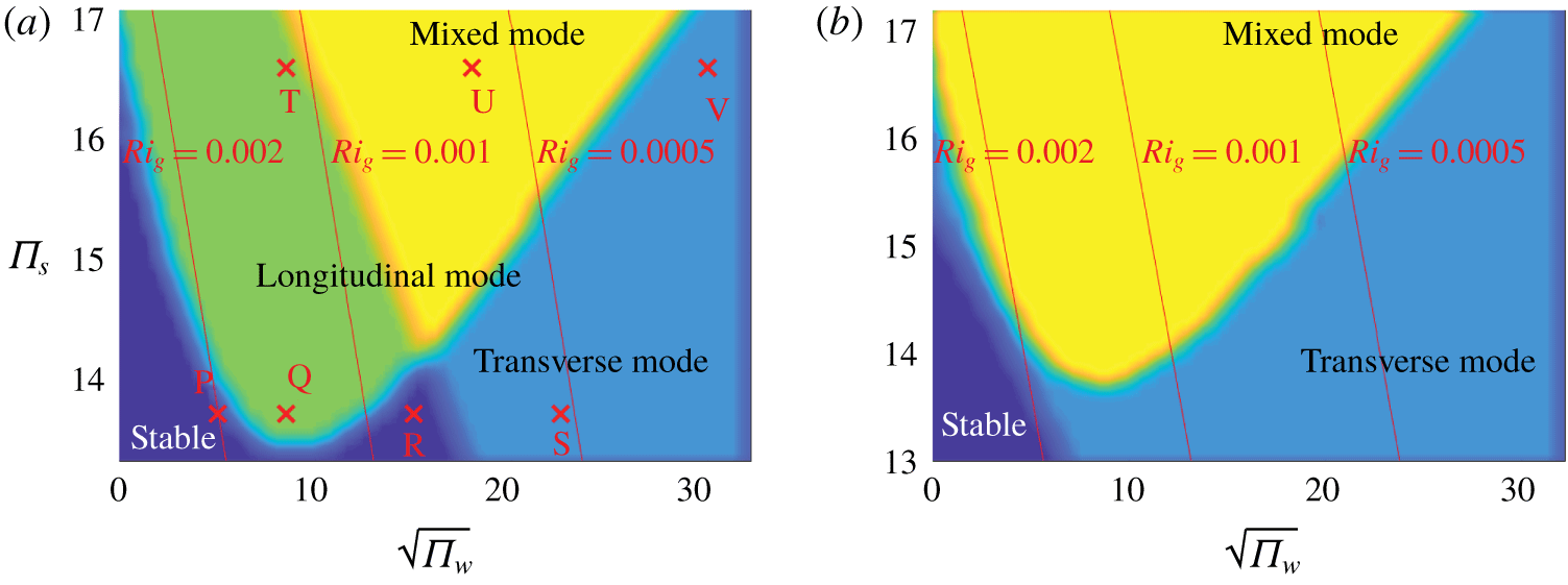
Regions of different modes at slope angles on the  $\unicode[STIX]{x1D6F1}_{s}-\unicode[STIX]{x1D6F1}_{w}$ space. (a)
 $\unicode[STIX]{x1D6FC}=67^{\circ }$; (b)
 $\unicode[STIX]{x1D6FC}=61^{\circ }$. The red lines are contours of
 $Ri_{g}$ number. The marked points P, Q, R, S all have
 $\unicode[STIX]{x1D6F1}_{s}=13.8$, whereas points T, U, V have
 $\unicode[STIX]{x1D6F1}_{s}=16.5$. The transitions among these states are shown in supplementary movies obtained from direct numerical simulation of (2.1)–(2.2) available at https://doi.org/10.1017/jfm.2019.1047. Movie 1: from Q (longitudinal mode) to R (stable); movie 2: from R (stable) to S (transverse mode); movie 3: from T (longitudinal mode) to U (mixed mode); and movie 4: from U (mixed mode) to V (transverse mode).

3.2 Mode transitions at steep slope angles
The aforementioned switching of the dominant instability from the longitudinal mode to transverse mode occurring at the steep angle of  $\unicode[STIX]{x1D6FC}=67^{\circ }$ is investigated here in more detail. Figure 5(a) shows that the dominant instability mode is a complex function of both parameters
 $\unicode[STIX]{x1D6F1}_{w},\unicode[STIX]{x1D6F1}_{s}$. For a fixed value of
 $\unicode[STIX]{x1D6F1}_{s}<16.5$, the base flow is initially stable for
 $\unicode[STIX]{x1D6F1}_{w}=0$, then becomes linearly unstable to the longitudinal mode with increasing
 $\unicode[STIX]{x1D6F1}_{w}$. When
 $\unicode[STIX]{x1D6F1}_{w}$ continues to grow, depending on the value of
 $\unicode[STIX]{x1D6F1}_{s}$, the flow then becomes either stable again (
 $\unicode[STIX]{x1D6F1}_{s}<14$) or susceptible to both longitudinal and transverse instability modes (
 $\unicode[STIX]{x1D6F1}_{s}>14$). For
 $\unicode[STIX]{x1D6F1}_{w}$ large enough, however, the dominant instability becomes the transverse mode. The effect of flow stabilisation despite lowering of
 $Ri_{g}$ and the subsequent mode switching can be observed in the marked points P, Q, R, S, T, U, V shown in figure 5(a). These transitions predicted by linear modal analysis can also be observed in the four supplementary movies obtained from direct numerical simulation data: keeping
 $\unicode[STIX]{x1D6F1}_{s}$ constant at 13.8, movie 1 demonstrates the stabilising transition from Q to R, whereas movie 2 shows the emergence of the transverse mode by moving from R to S; at the higher value
 $\unicode[STIX]{x1D6F1}_{s}=16.5$, movie 3 displays how the mixed mode appears by transition from T to U, whereas movie 4 indicates the weakening of the longitudinal mode when moving from U to V. The stabilising effect of a flow parameter that is generally considered to be monotonically destabilising has also been reported by Gollub & Benson (Reference Gollub and Benson1980), where an increase of the Rayleigh number was found to reduce the complexity of convective flow patterns for certain initial mean flow fields.
The same contour plot for a slightly smaller angle of  $\unicode[STIX]{x1D6FC}=61^{\circ }$ is shown in figure 5(b), which indicates that the region of longitudinal mode has completely vanished at this angle, in agreement with the known fact that the longitudinal instability is dominated at smaller slope angles.
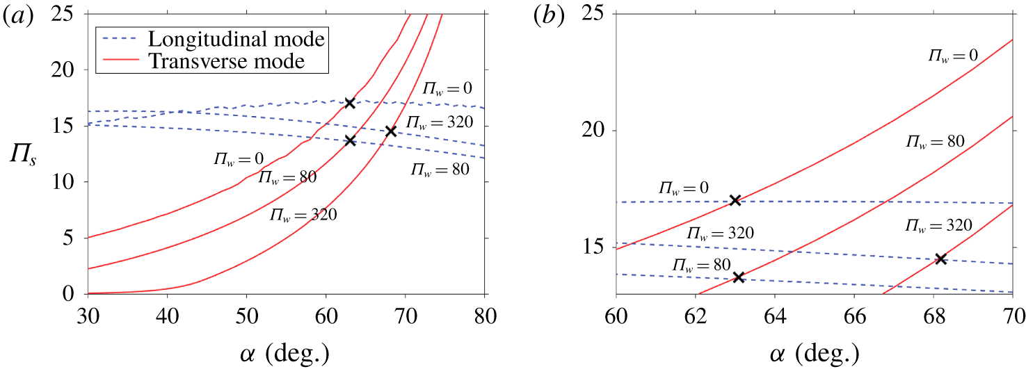
The  $\unicode[STIX]{x1D6F1}_{s}-\unicode[STIX]{x1D6FC}$ instability map for katabatic slope flows at
 $Pr=0.71$ for different ambient wind values measured by
 $\unicode[STIX]{x1D6F1}_{w}$. The crosses mark the angle at which both instability modes have the same critical
 $\unicode[STIX]{x1D6F1}_{s}$ threshold. Panel (b) zooms into the angle range in which the transition from transverse to longitudinal mode happens.

3.3 Stability at different slope angles
As pointed out in the previous subsection, the most dangerous modes at each slope angle  $\unicode[STIX]{x1D6FC}$ and parameter couples
 $\unicode[STIX]{x1D6F1}_{s},\unicode[STIX]{x1D6F1}_{w}$ either have pure along-slope (longitudinal mode) or pure cross-slope gradients (transverse mode). A plot of the critical
 $\unicode[STIX]{x1D6F1}_{s}$ required for the onset of each instability mode at a specific slope angle
 $\unicode[STIX]{x1D6FC}$ and wind forcing number
 $\unicode[STIX]{x1D6F1}_{w}$ is shown in figure 6. The effect of the ambient wind on the transition slope angle
 $\unicode[STIX]{x1D6FC}_{t}$ at which the dominant instability mode switches from the transverse to longitudinal mode can be clearly observed: due to the stabilising effect of increasing ambient wind forcing on the longitudinal mode as discussed previously, for wind forcing number
 $\unicode[STIX]{x1D6F1}_{w}$ sufficiently large,
 $\unicode[STIX]{x1D6FC}_{t}$ increases beyond the value of
 $62^{\circ }$ found by Xiao & Senocak (Reference Xiao and Senocak2019) in the absence of ambient wind
 $\unicode[STIX]{x1D6F1}_{w}=0$. The monotonic destabilising effect of growing
 $\unicode[STIX]{x1D6F1}_{w}$ on the transverse mode, i.e. a lowering of its critical stability threshold over all shown angles, is also clearly visible. In particular, for slope angles
 $\unicode[STIX]{x1D6FC}<40^{\circ }$ and
 $\unicode[STIX]{x1D6F1}_{w}=320$, we can notice that the base flow profile is unstable to the transverse mode even for very small surface cooling, as evidenced by the threshold
 $\unicode[STIX]{x1D6F1}_{s}$ value close to zero.
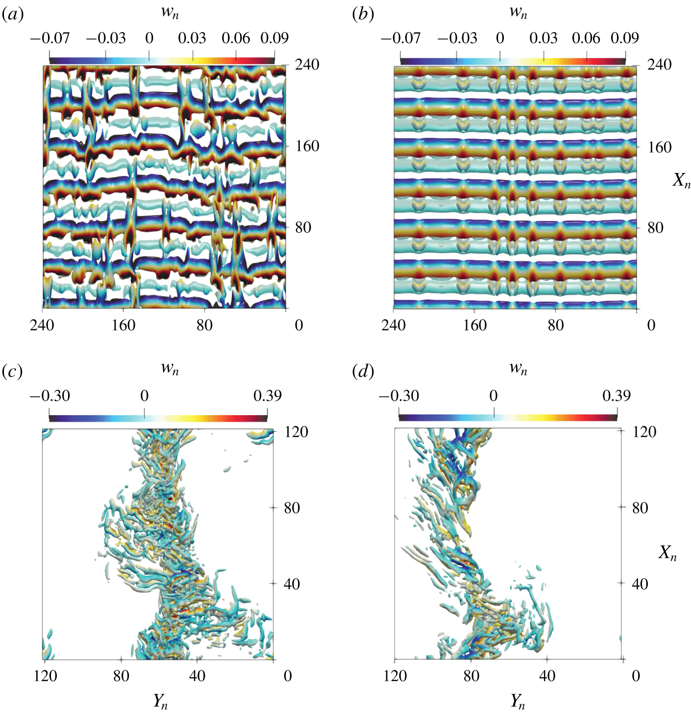
 $Q$-contour visualisations of mixed-mode instabilities. Colour represents the slope-normal velocity. (a,b)
 $\unicode[STIX]{x1D6FC}=67^{\circ }$ at constant
 $Ri_{g}\approx 5.25\times 10^{-4}$: (a)
 $\unicode[STIX]{x1D6F1}_{s}=36.77$,
 $\unicode[STIX]{x1D6F1}_{w}=0$; (b)
 $\unicode[STIX]{x1D6F1}_{s}=18$,
 $\unicode[STIX]{x1D6F1}_{w}=320$. (c,d)
 $\unicode[STIX]{x1D6FC}=5^{\circ }$ at constant
 $Ri_{g}=1.14\times 10^{-3}$: (c)
 $\unicode[STIX]{x1D6F1}_{s}=25$,
 $\unicode[STIX]{x1D6F1}_{w}=0$; (d)
 $\unicode[STIX]{x1D6F1}_{s}=19.8$,
 $\unicode[STIX]{x1D6F1}_{w}=320$. Main slope flow direction is from top to bottom.

3.4 Mixed instability mode
For a steep slope angle of  $\unicode[STIX]{x1D6FC}=67^{\circ }$, when
 $\unicode[STIX]{x1D6F1}_{s}$ is sufficiently large, figure 6 shows that for ambient wind values corresponding to
 $\unicode[STIX]{x1D6F1}_{w}=0,320$, both the transverse and longitudinal modes have positive growth rates. In order to visualise the flow field at these conditions, the Navier–Stokes equations (2.1)–(2.2) for katabatic slope flows are solved using a Cartesian mesh, three-dimensional, buoyancy-driven incompressible flow solver (Jacobsen & Senocak Reference Jacobsen and Senocak2013). The settings for the direct numerical simulations are the same as adopted in Xiao & Senocak (Reference Xiao and Senocak2019), i.e. the simulation domain is chosen to be large enough to capture multiple vortex rolls along both cross-slope and along-slope directions, and the mesh resolution ensures that there are at least two points per length scale
 $l_{0}$ in each direction.
To study the combined effect of the parameters  $\unicode[STIX]{x1D6F1}_{w},\unicode[STIX]{x1D6F1}_{s}$ on the mixed mode compared to the
 $Ri_{g}$ number, we have chosen configurations at the same slope angle
 $\unicode[STIX]{x1D6FC}=67^{\circ }$ and the same
 $Ri_{g}$ number, but with different combinations of
 $\unicode[STIX]{x1D6F1}_{w},\unicode[STIX]{x1D6F1}_{s}$ determined from (3.6). The first flow case contains no ambient wind and has
 $\unicode[STIX]{x1D6F1}_{s}=36.77$, whereas the second case has a wind forcing number of
 $\unicode[STIX]{x1D6F1}_{w}=320$ and a smaller
 $\unicode[STIX]{x1D6F1}_{s}=18$. An instantaneous visualisation of the results via the contour of the
 $Q$-criterion (Hunt, Wray & Moin Reference Hunt, Wray and Moin1988) is shown in figure 7(a,b), where the contour values used to obtain the plots are the same. It can clearly be seen that the flow field corresponding to the larger stratification perturbation
 $\unicode[STIX]{x1D6F1}_{s}=36.77$ is more unstable than its counterpart at the same
 $Ri_{g}$ number with a non-zero wind forcing number
 $\unicode[STIX]{x1D6F1}_{w}=320$. This serves as another confirmation of the result obtained from linear stability analysis as shown in figure 2, where the maximal growth rate of instabilities declines along the
 $Ri$-contour when
 $\unicode[STIX]{x1D6F1}_{s}$ is reduced and
 $\unicode[STIX]{x1D6F1}_{w}$ is increased. The same comparison is made for a shallow slope with
 $\unicode[STIX]{x1D6FC}=5^{\circ }$, shown in figure 7(c,d). In the first flow configuration, we have
 $\unicode[STIX]{x1D6F1}_{s}=25$ without ambient wind, whereas the second configuration has a smaller
 $\unicode[STIX]{x1D6F1}_{s}=19.8$ but a non-zero wind forcing number of
 $\unicode[STIX]{x1D6F1}_{w}=320$; both flows have the same
 $Ri_{g}$ number. Similar to the steep slope case, it is evident that the first flow field with the larger stratification perturbation
 $\unicode[STIX]{x1D6F1}_{s}=25$ looks more unstable and contains smaller eddies than the second flow at the same
 $Ri_{g}$ number with a non-zero wind forcing number
 $\unicode[STIX]{x1D6F1}_{w}=320$. Thus, it appears that for a fixed
 $Ri_{g}$, the surface buoyancy has a stronger destabilisation effect than the ambient wind higher aloft.
4 Conclusions
We performed a linear stability analysis of the extended Prandtl model (Lykosov & Gutman Reference Lykosov and Gutman1972) for katabatic slope flows to investigate the effect of a constant downslope ambient wind on the stability behaviour of slope flows on an infinitely wide planar surface cooled from below. Our analysis has led to a new dimensionless number that we interpret as the ratio of kinetic energy of the ambient wind to the damping of kinetic energy in slope flows due to the combined action of viscosity and stable stratification. We designated this new dimensionless number  $\unicode[STIX]{x1D6F1}_{w}$ the wind forcing parameter. We then demonstrated that the stability behaviour of katabatic slope flows under the extended Prandtl model at a constant slope angle and Prandtl number is completely defined by
 $\unicode[STIX]{x1D6F1}_{w}$ and the stratification perturbation parameter (
 $\unicode[STIX]{x1D6F1}_{s}$) that we have introduced earlier in Xiao & Senocak (Reference Xiao and Senocak2019). The extended Prandtl model also enables us to show analytically that the gradient Richardson number (
 $Ri_{g}$) is a function depending on multiple parameters.
 $Ri_{g}$ is a monotonic decreasing function of
 $\unicode[STIX]{x1D6F1}_{s}$ and
 $\unicode[STIX]{x1D6F1}_{w}$ at a given slope angle and
 $Pr$ number. We conducted direct numerical simulations to further demonstrate that dynamically different slope flows do emerge under the same
 $Ri_{g}$ and the same slope angle
 $\unicode[STIX]{x1D6FC}$. Collectively, our results show that a single
 $Ri_{g}$ criterion is ineffective to characterise the stability behaviour katabatic slope flows under the original or extended Prandtl model.
The types of flow instabilities that occur under the extended Prandtl model are the same as the stationary transverse mode and travelling longitudinal mode that were uncovered in Xiao & Senocak (Reference Xiao and Senocak2019), but their characteristics can exhibit a complex behaviour as a result of ambient wind forcing. When  $\unicode[STIX]{x1D6F1}_{s}$ is held constant, ambient wind forcing monotonically destabilises the stationary transverse mode. For the travelling longitudinal instability at steep slope angles, however, an increase of ambient wind forcing, within a certain range of
 $\unicode[STIX]{x1D6F1}_{w}$ values, can stabilise the entire flow configuration until its value becomes sufficiently large to trigger the dormant mode of instability, which, in this case, is the stationary transverse instability. This observation runs counter to the currently held assumption that a decrease in
 $Ri_{g}$ always destabilises the base flow. Thus, it further supports our argument that any stability criterion based solely on
 $Ri_{g}$ number is insufficient for slope flows under the original or the extended Prandtl model. Future subgrid-scale parameterisation schemes for stably stratified slope flows would benefit from taking into account the dependency of flow stability on the dimensionless multiparameter space that we have laid out in the present work.
Acknowledgements
Research was sponsored by the Army Research Office and was accomplished under grant no. W911NF-17-1-0564 with Dr J. Baryzk as the programme manager, and in part by the National Science Foundation under award no. 1936445. The views and conclusions contained in this document are those of the authors and should not be interpreted as representing the official policies, either expressed or implied, of the Army Research Office or the U.S. Government. The U.S. Government is authorised to reproduce and distribute reprints for Government purposes notwithstanding any copyright notation herein.
Declaration of interests
The authors report no conflict of interest.
Supplementary movies
Supplementary movies are available at https://doi.org/10.1017/jfm.2019.1047.