1 Introduction
At the 1961 international colloquium in Marseille and following Oboukhov (Reference Oboukhov1962), Kolmogorov revised his 1941 theory or K41 (Kolmogorov Reference Kolmogorov1941a
), to address an issue first raised by Landau (see for example Landau & Lifshitz Reference Landau and Lifshitz1987) shortly after K41 was published, namely the variation in the mean turbulent kinetic energy dissipation rate
 $\overline{\unicode[STIX]{x1D716}}$
induced by the large-scale motion. This revision, usually referred to as K62 (Kolmogorov Reference Kolmogorov1962), is known as the ‘refined’ similarity hypothesis. For over almost 60 years and with a few exceptions (e.g. Kraichnan Reference Kraichnan1974; Qian Reference Qian2000; Lundgren Reference Lundgren2002; McComb Reference McComb2014), the current dominant view is that the properties of small scale turbulence comply with K62. However, this view is currently being challenged (e.g. Antonia et al.
Reference Antonia, Tang, Djenidi and Danaila2015; Tang et al.
Reference Tang, Antonia, Djenidi, Abe, Zhou, Danaila and Zhou2015a
,Reference Tang, Antonia, Djenidi and Zhou
b
; Antonia et al.
Reference Antonia, Djenidi, Danaila and Tang2017) on the basis that before the effect of intermittency can be adequately assessed, i.e. before one can unambiguously decide between K41 and K62 (a sine qua non requirement of both K41 and K62 is that the Reynolds number is very large) one must first ensure that the finite Reynolds number (FRN) effect is no longer active.
A study by Antonia & Burattini (Reference Antonia and Burattini2006) (see also Zhou et al.
Reference Zhou, Antonia, Danaila and Anselmet2000) showed that
 $\overline{(\unicode[STIX]{x1D6FF}u)^{3}}$
(the third-order moment of the longitudinal velocity increment
 $\unicode[STIX]{x1D6FF}u=(u(r)-u(0))$
, where
 $r$
is the separation between two points separated in
 $x$
, the longitudinal direction; the overbar denotes time and/or spatial averaging) approaches
 $-4\overline{\unicode[STIX]{x1D716}}r/5$
in the inertial range as the Taylor microscale Reynolds number,
 $Re_{\unicode[STIX]{x1D706}}$
, reaches large values in both decaying and forced homogeneous and isotropic turbulence (HIT). More recently, Tchoufag, Sagaut & Cambon (Reference Tchoufag, Sagaut and Cambon2012) confirmed this trend by carrying out an eddy damped quasi-normal Markovian (EDQNM) calculation of the Lin equation. It should be stressed that
 $\overline{(\unicode[STIX]{x1D6FF}u)^{3}}=-4\overline{\unicode[STIX]{x1D716}}r/5$
is the so-called four-fifths law, derived by Kolmogorov (Reference Kolmogorov1941b
) from the Navier–Stokes equation and thus is rigorous and exact when
 $Re_{\unicode[STIX]{x1D706}}$
is very large. Accordingly, these two studies reveal a clear Reynolds number effect (coined ‘the finite Reynolds number or FRN effect’; see Qian Reference Qian1997, Reference Qian1999; Danaila et al.
Reference Danaila, Anselmet, Zhou and Antonia1999; Lindborg Reference Lindborg1999; Antonia & Burattini Reference Antonia and Burattini2006) otherwise ignored or, most likely, mistaken for the effect of the intermittency of
 $\unicode[STIX]{x1D716}$
on the small-scale motion. Further, recent studies (Antonia et al.
Reference Antonia, Tang, Djenidi and Danaila2015; Tang et al.
Reference Tang, Antonia, Djenidi, Abe, Zhou, Danaila and Zhou2015a
,Reference Tang, Antonia, Djenidi and Zhou
b
) extended the assessment of the FRN effect on the skewness factor,
 $S$
, of the longitudinal velocity derivative
 $(\unicode[STIX]{x2202}u/\unicode[STIX]{x2202}x)$
in several turbulent flows. These latter studies indicate that
 $S$
approaches the same constant, approximately
 $-0.55$
, in all flows investigated when
 $Re_{\unicode[STIX]{x1D706}}$
increases. Approximately the same value (
 $-0.53$
) was obtained in the EDQNM simulation of HIT by Meldi & Sagaut (Reference Meldi and Sagaut2013a
) and much earlier by Qian (Reference Qian1994). This result, i.e. the approach toward an asymptotic constant value for
 $S$
with an increasing
 $Re_{\unicode[STIX]{x1D706}}$
, is consistent with K41, which predicts that
 $S$
is a universal constant; under the framework of K62,
 $-S\sim Re_{\unicode[STIX]{x1D706}}^{\unicode[STIX]{x1D6FC}}$
, where
 $\unicode[STIX]{x1D6FC}$
is a small positive real number (
 $0\leqslant \unicode[STIX]{x1D6FC}\leqslant 1$
).
It is worth stressing that despite their conflicting predictions, K41 and K62 assume that the Reynolds number is very large and local isotropy is satisfied (following a long energy cascade process). These two requirements must be met before one can test these theories. The second requirement would exclude certain flows or flow regions, for example, and as noted by Kolmogorov, those in the vicinity of boundaries. In this context, it is somewhat surprising that data obtained in the atmospheric shear layer (ASL) (see Sreenivasan & Antonia Reference Sreenivasan and Antonia1997) where
 $Re_{\unicode[STIX]{x1D706}}$
can be large were used to test K41 and K62. Lack of information on the ASL layer thickness
 $\unicode[STIX]{x1D6FF}$
makes it very difficult to estimate
 $y/\unicode[STIX]{x1D6FF}$
(
 $y$
is the height above the ground or ocean surface). Accordingly, one cannot rule out that the ASL data as reported in Sreenivasan & Antonia (Reference Sreenivasan and Antonia1997) and often measured at only a few metres above the surface are contaminated by the near-surface effects (Djenidi et al.
Reference Djenidi, Antonia, Talluru and Abe2017a
; Meldi & Sagaut Reference Meldi and Sagaut2017). ASL data are not immune from the FRN effect (as noted in Sreenivasan & Antonia Reference Sreenivasan and Antonia1997) as well as the influence of the strong shear. In addition, another open question is whether the threshold value for
 $Re_{\unicode[STIX]{x1D706}}$
for which FRN effects can be safely neglected is the same for every flow statistical quantity. Numerical results by Meldi & Sagaut (Reference Meldi and Sagaut2013a
) seem to indicate that this value increases with higher-order statistics. Tang et al. (Reference Tang, Antonia, Djenidi, Danaila and Zhou2017) who investigated the effect of the FRN effect in the scaling range exponent
 $\unicode[STIX]{x1D701}_{n}$
(
 $\overline{(\unicode[STIX]{x1D6FF}u)^{n}}\sim r^{\unicode[STIX]{x1D701}_{n}}$
) showed that the magnitude of
 $\unicode[STIX]{x1D701}_{n}$
increases, strictly the maximum value of (
 $\overline{(\unicode[STIX]{x1D6FF}u)^{n}}r^{-\unicode[STIX]{x1D701}_{n}}$
), as
 $Re_{\unicode[STIX]{x1D706}}$
increases and the rate of increase depends on the order
 $n$
.
In the present study, we investigate, via EDQNM calculations, the FRN effect in freely decaying HIT. Particular emphasis is on the behaviour of the flatness factor,
 $F$
, of
 $\unicode[STIX]{x2202}u/\unicode[STIX]{x2202}x$
over a very large range for
 $Re_{\unicode[STIX]{x1D706}}$
. A similar EDQNM analysis on the velocity derivative skewness factor,
 $S$
, was reported in Meldi & Sagaut (Reference Meldi and Sagaut2013a
). Since, conversely to
 $S$
,
 $F$
cannot be directly computed from the EDQNM calculations, the FRN effect on
 $F$
is investigated by assessing the FRN effect on a new analytic expression for
 $F$
, rigorously derived from the Navier–Stokes equations (Djenidi et al.
Reference Djenidi, Danaila, Antonia and Tang2017b
) for HIT. The novelty of the present contribution lies in the ability to assess the FRN effect when
 $Re_{\unicode[STIX]{x1D706}}$
varies from 200 to
 $5\times 10^{5}$
. This is possible due to the minimal computational resources required by the EDQNM simulations. This range of
 $Re_{\unicode[STIX]{x1D706}}$
, which exceeds three decades, allows for an unambiguous identification of the FRN effect on both
 $S$
and
 $F$
, with the expectation that FRN effects identified via EDQNM are at least comparable if not identical to the behaviour described by the Navier–Stokes equations. Such an extended range of
 $Re_{\unicode[STIX]{x1D706}}$
cannot be reached, either experimentally or with conventional direct numerical simulation (DNS).
2 Flatness factor of
 $\unicode[STIX]{x2202}u/\unicode[STIX]{x2202}x$

2.1 A rigorous analytic expression
The flatness factor of
 $\unicode[STIX]{x2202}u/\unicode[STIX]{x2202}x$
is defined as
 $$\begin{eqnarray}F=\frac{\overline{(\unicode[STIX]{x2202}u/\unicode[STIX]{x2202}x)^{4}}}{\overline{(\unicode[STIX]{x2202}u/\unicode[STIX]{x2202}x)^{2}}^{2}}.\end{eqnarray}$$
However, starting with the equation for
 $\overline{(\unicode[STIX]{x1D6FF}u)^{3}}$
(as first written by Hill (Reference Hill2001)), applying self-similarity (or scale invariance) and taking the limit
 $r\rightarrow 0$
, Djenidi et al. (Reference Djenidi, Danaila, Antonia and Tang2017b
) derived the following analytic equation for
 $F$
:
 $$\begin{eqnarray}F+\frac{10}{3}\unicode[STIX]{x1D6FE}_{1}-\frac{20}{3}\frac{\unicode[STIX]{x1D6FE}_{2}}{Re_{\unicode[STIX]{x1D706}}}\simeq -\unicode[STIX]{x1D6FC}\frac{S}{Re_{\unicode[STIX]{x1D706}}},\end{eqnarray}$$
where
 $\unicode[STIX]{x1D6FE}_{1}=(\unicode[STIX]{x1D706}^{4}/u^{\prime 4})\overline{(\unicode[STIX]{x2202}u/\unicode[STIX]{x2202}x)^{2}(\unicode[STIX]{x2202}^{2}p/\unicode[STIX]{x2202}x^{2})}$
,
 $\unicode[STIX]{x1D6FE}_{2}=(\unicode[STIX]{x1D706}^{5}/u^{\prime 3})\overline{\tilde{\unicode[STIX]{x1D716}}_{HIT}(\unicode[STIX]{x2202}^{3}u/\unicode[STIX]{x2202}x^{3})}$
with
 $\tilde{\unicode[STIX]{x1D716}}_{HIT}=(7/6)(\unicode[STIX]{x2202}u/\unicode[STIX]{x2202}x)^{2}-(2/3)(\unicode[STIX]{x2202}u/\unicode[STIX]{x2202}y)^{2}$
(
 $p$
is the kinematic pressure fluctuation) and
 $\unicode[STIX]{x1D6FC}$
is a numerical (dimensionless) constant. In this expression
 $\unicode[STIX]{x1D706}$
and
 $u^{\prime }$
were used as scaling variables. If the Kolmogorov scales are used, equation (2.2) can be replaced by
 $$\begin{eqnarray}F+750[\unicode[STIX]{x1D6FE}_{1,K}-4\unicode[STIX]{x1D6FE}_{2,K}]\simeq -\frac{100}{3}\frac{S}{Re_{\unicode[STIX]{x1D706}}},\end{eqnarray}$$
where the subscript
 $K$
represents Kolmogorov normalisation. The second and third terms on the left-hand side of (2.2) or (2.3) represent the actions of pressure and viscosity, respectively. Noting that
 $S/Re_{\unicode[STIX]{x1D706}}\rightarrow 0$
, irrespectively of whether
 $S$
is constant or varies like
 $Re_{\unicode[STIX]{x1D706}}^{\unicode[STIX]{x1D6FC}}$
(
 $0\leqslant \unicode[STIX]{x1D6FC}\leqslant 1$
), equation (2.2) can be written as
 $$\begin{eqnarray}F\simeq -\frac{10}{3}\unicode[STIX]{x1D6FE}_{1}+\frac{20}{3}\frac{\unicode[STIX]{x1D6FE}_{2}}{Re_{\unicode[STIX]{x1D706}}}\end{eqnarray}$$
for large
 $Re_{\unicode[STIX]{x1D706}}$
. In Djenidi et al. (Reference Djenidi, Danaila, Antonia and Tang2017b
), the second term on the right-hand side of (2.4) was assumed to be negligible when
 $Re_{\unicode[STIX]{x1D706}}$
becomes very large. Since there is no a priori justification for this, it has been retained.
It is important to stress that (2.2), a rigorous model-free expression for
 $F$
, is derived from the Navier–Stokes equations under the assumption of self-similarity. Note though that the presence of the pressure term makes it difficult, if not impossible, to test this expression experimentally. One must resort to direct numerical simulations (DNS). To date, the highest
 $Re_{\unicode[STIX]{x1D706}}$
reached by DNS in forced HIT (Ishihara et al.
Reference Ishihara, Kaneda, Yokokawa, Itakura and Uno2007) is approximately 1150. The maximum
 $Re_{\unicode[STIX]{x1D706}}$
for DNS of freely decaying HIT is smaller, because of lingering effects of initial conditions and confinement effects (Meldi & Sagaut Reference Meldi and Sagaut2017), thus limiting the range of investigation of
 $Re_{\unicode[STIX]{x1D706}}$
. On the other hand,
 $Re_{\unicode[STIX]{x1D706}}$
of order
 $10^{5}$
can be achieved with EDQNM simulations of decaying HIT (Meldi & Sagaut Reference Meldi and Sagaut2013a
). However, this model calculates the time evolution of the energy spectrum
 $E$
in Fourier transform space, so that the terms of (2.4) cannot be directly obtained. Therefore, we use an analysis based on dimensional arguments on the statistical quantities available via EDQNM, which allows us to qualitatively assess their
 $Re$
-dependence. This dimensional analysis is consistent with the assumption of self-similarity used to derive (2.2).
2.2 Dimensional arguments
While the definitions of the coefficients
 $\unicode[STIX]{x1D6FE}_{1}$
and
 $\unicode[STIX]{x1D6FE}_{2}$
are clear in physical space, their formulation in a spectral frame of reference is elusive. The second-order link between statistics in the physical and spectral spaces is obtained by comparing the Kármán–Howarth equation with the Lin equation. For third-order statistics, the link is provided using the time evolution equation for the energy dissipation rate
 $\overline{\unicode[STIX]{x1D716}}$
in the spectral domain (Meldi & Sagaut Reference Meldi and Sagaut2013a
) and the vorticity equation in physical space. Restricting the analysis to purely isotropic turbulence, both equations exhibit a destruction term which is determined by a spectral integration including a correct dimensional combination of the wavenumber
 $k$
and the energy spectrum
 $E(k,t)$
. In particular, the expressions are
 $\overline{\unicode[STIX]{x1D716}}\propto \overline{(\unicode[STIX]{x2202}u/\unicode[STIX]{x2202}x)(\unicode[STIX]{x2202}u/\unicode[STIX]{x2202}x)}\propto \int k^{2}E\,\text{d}k$
and
 $G(\overline{\unicode[STIX]{x1D716}}^{2}/{\mathcal{K}})\propto \overline{(\unicode[STIX]{x2202}^{2}u/\unicode[STIX]{x2202}x^{2})(\unicode[STIX]{x2202}^{2}u/\unicode[STIX]{x2202}x^{2})}\propto \int k^{4}E\,\text{d}k$
for the energy dissipation rate and the palinstrophy, respectively. A corresponding relation between physical and spectral spaces is missing for fourth-order statistics. However, the dimensions of the terms in the equation for
 $\overline{(\unicode[STIX]{x1D6FF}u)^{3}}$
used to derived expression (2.2) are expressed in terms of the metre
 $m$
and second
 $s$
. Further, these terms can be represented spectrally. For example, let us consider the pressure term and follow Djenidi et al. (Reference Djenidi, Danaila, Antonia and Tang2017b
) who, after applying the Cauchy–Schwarz theorem, obtained the following expression:
 $$\begin{eqnarray}\left|\overline{\left(\frac{\unicode[STIX]{x2202}u}{\unicode[STIX]{x2202}x}\right)^{2}\frac{\unicode[STIX]{x2202}^{2}p}{\unicode[STIX]{x2202}x^{2}}}\right|\leqslant \overline{\left(\frac{\unicode[STIX]{x2202}u}{\unicode[STIX]{x2202}x}\right)^{4}}^{1/2}\overline{\left(\frac{\unicode[STIX]{x2202}^{2}p}{\unicode[STIX]{x2202}x^{2}}\right)^{2}}^{1/2},\end{eqnarray}$$
which finally leads to (Djenidi et al. Reference Djenidi, Danaila, Antonia and Tang2017b )
 $$\begin{eqnarray}|\unicode[STIX]{x1D6FE}_{1}|=\frac{\unicode[STIX]{x1D706}^{4}}{u^{\prime 4}}\left|\overline{\left(\frac{\unicode[STIX]{x2202}u}{\unicode[STIX]{x2202}x}\right)^{2}\left(\frac{\unicode[STIX]{x2202}^{2}p}{\unicode[STIX]{x2202}x^{2}}\right)}\right|\leqslant F^{1/2}\left(\int _{0}^{\infty }k^{\ast 4}E_{p}^{\ast }(k^{\ast })\,\text{d}k^{\ast }\right)^{1/2},\end{eqnarray}$$
where the symbol
 $\ast$
represents normalisation using
 $\unicode[STIX]{x1D706}$
and
 $u^{\prime }$
as scaling variables. Considering that
 $p$
can be easily expressed in terms of
 $u$
, one can expect that
 $\unicode[STIX]{x1D6FE}_{1}$
may be expressed in terms of
 $k$
and
 $E(k)$
, as will be shown below. Since both terms on the right-hand side of (2.4) must have the same dimensions, then
 $\unicode[STIX]{x1D6FE}_{2}$
can, like
 $\unicode[STIX]{x1D6FE}_{1}$
, also be expressed in the spectral domain via dimensional arguments in terms of
 $k$
and
 $E(k)$
. For the sake of simplicity we assume that, under isotropy,
 $\overline{(\unicode[STIX]{x2202}u/\unicode[STIX]{x2202}y)^{2}}=2\overline{(\unicode[STIX]{x2202}u/\unicode[STIX]{x2202}x)^{2}}$
and
 $$\begin{eqnarray}\overline{\left(\frac{7}{6}\left(\frac{\unicode[STIX]{x2202}u}{\unicode[STIX]{x2202}x}\right)^{2}-\frac{2}{3}\left(\frac{\unicode[STIX]{x2202}u}{\unicode[STIX]{x2202}y}\right)^{2}\right)\frac{\unicode[STIX]{x2202}^{3}u}{\unicode[STIX]{x2202}x^{3}}}\sim \overline{\left(\frac{\unicode[STIX]{x2202}u}{\unicode[STIX]{x2202}x}\right)^{2}\frac{\unicode[STIX]{x2202}^{3}u}{\unicode[STIX]{x2202}x^{3}}}.\end{eqnarray}$$
We can now use dimensional arguments to derive
 $\unicode[STIX]{x1D6FE}_{1}$
and
 $\unicode[STIX]{x1D6FE}_{2}$
. First, we write
 $\unicode[STIX]{x1D6FE}_{1}\propto \overline{(\unicode[STIX]{x2202}u/\unicode[STIX]{x2202}x)^{2}(\unicode[STIX]{x2202}^{2}p/\unicode[STIX]{x2202}x^{2})}\approx \overline{(\unicode[STIX]{x2202}u/\unicode[STIX]{x2202}x)^{4}}=\unicode[STIX]{x1D709}_{1}$
, where we used the relation between
 $p$
and
 $u$
. We write
 $\unicode[STIX]{x1D6FE}_{1}\propto \unicode[STIX]{x1D709}_{1}$
, and note that
 $\overline{(\unicode[STIX]{x2202}u/\unicode[STIX]{x2202}x)^{4}}=\overline{(\unicode[STIX]{x2202}u/\unicode[STIX]{x2202}x)^{2}(\unicode[STIX]{x2202}u/\unicode[STIX]{x2202}x)^{2}}$
exhibits similarities with the spectral transforms of
 $\unicode[STIX]{x1D716}$
and
 $G$
. This term has dimensions of
 $[m^{0}\,s^{-4}]$
. Starting from the assumption that this term depends only on
 $k$
and
 $E$
, dimensional arguments lead to:
 $$\begin{eqnarray}\overline{\left(\frac{\unicode[STIX]{x2202}u}{\unicode[STIX]{x2202}x}\right)^{4}}\rightarrow \unicode[STIX]{x1D709}_{1}=a_{\unicode[STIX]{x1D709}_{1}}\int _{0}^{+\infty }k^{5}E^{2}\,\text{d}k.\end{eqnarray}$$
It should be stressed that we have investigated a number of different combinations of
 $k$
and
 $E$
complying with
 $[m^{0}\,s^{-4}]$
, including the dimensional quantities
 $\unicode[STIX]{x1D706}^{-1}\int _{0}^{\infty }k^{4}E^{2}\,\text{d}k$
and
 $\int _{0}^{\infty }k^{4}E_{p}(k)\,\text{d}k$
. The high Reynolds number behaviour of all these quantities, which is the subject of the present investigation, is identical.
A similar approach is employed to derive a spectral expression for the coefficient
 $\unicode[STIX]{x1D6FE}_{2}$
. The starting point is the quantity
 $\overline{(\unicode[STIX]{x2202}u/\unicode[STIX]{x2202}x)^{2}(\unicode[STIX]{x2202}^{3}u/\unicode[STIX]{x2202}x^{3})}$
, whose dimension is
 $[m^{-2}\,s^{-3}]$
. Again, dimensional arguments based on
 $k$
and
 $E$
yields:
 $$\begin{eqnarray}\overline{\left(\frac{\unicode[STIX]{x2202}u}{\unicode[STIX]{x2202}x}\right)^{2}\frac{\unicode[STIX]{x2202}^{3}u}{\unicode[STIX]{x2202}x^{3}}}\rightarrow \unicode[STIX]{x1D709}_{2}=a_{\unicode[STIX]{x1D709}_{2}}\int _{0}^{+\infty }k^{11/2}E^{3/2}\,\text{d}k.\end{eqnarray}$$
Finally, a third term is investigated. While it is not directly connected with the terms in (2.4), it is introduced to allow us to define a new invariant. This term can be obtained from the homogeneity condition:
 $$\begin{eqnarray}\frac{\unicode[STIX]{x2202}}{\unicode[STIX]{x2202}x}\overline{\left(\frac{\unicode[STIX]{x2202}u}{\unicode[STIX]{x2202}x}\right)^{2}\left(\frac{\unicode[STIX]{x2202}^{2}u}{\unicode[STIX]{x2202}x^{2}}\right)}=0,\end{eqnarray}$$
which implies that
 $\overline{(\unicode[STIX]{x2202}u/\unicode[STIX]{x2202}x)^{2}(\unicode[STIX]{x2202}^{3}u/\unicode[STIX]{x2202}x^{3})}\propto \overline{(\unicode[STIX]{x2202}^{2}u/\unicode[STIX]{x2202}x^{2})^{2}(\unicode[STIX]{x2202}u/\unicode[STIX]{x2202}x)}$
. Taking into account the exact relation
 $\overline{(\unicode[STIX]{x2202}u/\unicode[STIX]{x2202}x)^{3}}=\overline{(\unicode[STIX]{x2202}u/\unicode[STIX]{x2202}x)^{2}(\unicode[STIX]{x2202}u/\unicode[STIX]{x2202}x)}\rightarrow \int _{0}^{+\infty }k^{2}T\,\text{d}k$
and since the square of
 $(\unicode[STIX]{x2202}u/\unicode[STIX]{x2202}x)^{2}$
is linked to the square of the second derivative
 $(\unicode[STIX]{x2202}^{2}u/\unicode[STIX]{x2202}x^{2})^{2}$
via a
 $k^{2}$
term in spectral space (Pope Reference Pope2000), the following relation is obtained:
 $$\begin{eqnarray}\overline{\left(\frac{\unicode[STIX]{x2202}^{2}u}{\unicode[STIX]{x2202}x^{2}}\right)^{2}\frac{\unicode[STIX]{x2202}u}{\unicode[STIX]{x2202}x}}\rightarrow \unicode[STIX]{x1D709}_{3}=a_{\unicode[STIX]{x1D709}_{3}}\int _{0}^{+\infty }k^{4}T\,\text{d}k.\end{eqnarray}$$
Thus, we can introduce a new coefficient
 $\unicode[STIX]{x1D6FE}_{3}\propto \unicode[STIX]{x1D709}_{3}$
, whose behaviour will be investigated in § 4.4. The expressions for
 $\unicode[STIX]{x1D709}_{1}$
and
 $\unicode[STIX]{x1D709}_{2}$
allow us to ascertain the Reynolds number behaviour of the flatness expression coefficients
 $\unicode[STIX]{x1D6FE}_{1}$
,
 $\unicode[STIX]{x1D6FE}_{2}$
. As will be seen later, the coefficient
 $\unicode[STIX]{x1D6FE}_{3}$
allows us to define and investigate a new invariant. It can be defined similarly to
 $\unicode[STIX]{x1D6FE}_{2}$
because of dimensional analogy between
 $\unicode[STIX]{x1D709}_{2}$
and
 $\unicode[STIX]{x1D709}_{3}$
. Thus, finally, the results of the dimensional argument analysis are:
 $$\begin{eqnarray}\unicode[STIX]{x1D6FE}_{1}=-\frac{\unicode[STIX]{x1D706}^{4}}{\left({\textstyle \frac{2}{3}}{\mathcal{K}}\right)^{2}}\unicode[STIX]{x1D709}_{1},\quad \unicode[STIX]{x1D6FE}_{2}=\frac{\unicode[STIX]{x1D706}^{5}}{\left({\textstyle \frac{2}{3}}{\mathcal{K}}\right)^{3/2}}\unicode[STIX]{x1D709}_{2},\quad \unicode[STIX]{x1D6FE}_{3}=\frac{\unicode[STIX]{x1D706}^{5}}{\left({\textstyle \frac{2}{3}}{\mathcal{K}}\right)^{3/2}}\unicode[STIX]{x1D709}_{3},\end{eqnarray}$$
where
 ${\mathcal{K}}$
is the turbulent kinetic energy. Interestingly, Tang et al. (Reference Tang, Antonia, Djenidi, Danaila and Zhou2018) recently showed that the term
 $\unicode[STIX]{x1D6FE}_{2}/Re_{\unicode[STIX]{x1D706}}$
in (2.4) becomes negligible as
 $Re_{\unicode[STIX]{x1D706}}$
increases. Thus, for large
 $Re_{\unicode[STIX]{x1D706}}$
, equation (2.4) leads to
 $F\approx \unicode[STIX]{x1D6FE}_{1}$
, and the following approximation can be obtained (Djenidi et al.
Reference Djenidi, Danaila, Antonia and Tang2017b
):
 $$\begin{eqnarray}F\leqslant \int _{0}^{\infty }k^{\ast 4}E_{p}^{\ast }(k^{\ast })\,\text{d}k^{\ast }.\end{eqnarray}$$
Since the right-hand side of this expression can be explicitly calculated using the EDQNM model (Meldi & Sagaut Reference Meldi and Sagaut2013b
), we will also assess its
 $Re_{\unicode[STIX]{x1D706}}$
-behaviour.
3 The EDQNM model
The eddy damped quasi-normal Markovian (EDQNM) model (Orszag Reference Orszag1970; Lesieur Reference Lesieur1997; Sagaut & Cambon Reference Sagaut and Cambon2018) is introduced in the present section. The model numerically resolves a discretisation in the spectral space (wavenumber
 $k$
) of the Lin equation, which describes the time evolution of the energy spectrum
 $E(k,t)$
:
 $$\begin{eqnarray}\frac{\unicode[STIX]{x2202}E(k,t)}{\unicode[STIX]{x2202}t}+2\unicode[STIX]{x1D708}k^{2}E(k,t)=T(k,t),\end{eqnarray}$$
where
 $\unicode[STIX]{x1D708}$
is the molecular viscosity of the fluid and
 $T(k,t)$
is the nonlinear energy transfer. The EDQNM closure acts on the evolution equation of
 $T$
via two important approximations:
(i) the fourth-order cumulants, which represent the deviation of the velocity derivative pdf from a Gaussian distribution, are approximated using an eddy damping term (eddy damping hypothesis);
(ii) time integration is simplified via a Markovianisation procedure.
A closed expression for the nonlinear energy transfer
 $T(k,t)$
is obtained via shell integration of radius
 $k$
:
 $$\begin{eqnarray}T_{EDQNM}=\int _{p+q=k}\unicode[STIX]{x1D6E9}_{kpq}gE(q,t)[E(p,t)pk^{2}-E(k,t)p^{3}]\frac{\text{d}p\,\text{d}q}{pq},\end{eqnarray}$$
where
 $\unicode[STIX]{x1D6E9}_{kpq}$
is a characteristic time resulting from the Markovian approximation and
 $g$
is a geometric function.
The two underlying hypotheses used to obtain the closed expression (3.2) for the nonlinear energy transfer
 $T$
are well verified and their effect is expected to be very small, if not negligible, when compared with FRN effects which are presently investigated. Indeed, the Markovianisation hypothesis is an accurate approximation when a clear separation is observed between the turbulent characteristic time scale and the turnover time scale of the physical quantities investigated. The present analysis clearly satisfies this condition since the physical quantities investigated are intimately associated with the dissipative scales, which, considering the large values of
 $Re_{\unicode[STIX]{x1D706}}$
used, are well separated from the large scales. Further, the eddy damping hypothesis provides an accurate representation of fourth-order cumulants. This can be verified by comparing the present predicted velocity derivative skewness
 $S$
with the experimental data (see figure 1). The data reported in figure 1 have been collected from the relatively recent reappraisal of
 $S$
in various turbulent flows (Antonia et al.
Reference Antonia, Tang, Djenidi and Danaila2015), which includes a comprehensive overview of results reported in the literature; only a sample, for which
 $Re_{\unicode[STIX]{x1D706}}\geqslant 200$
, is shown in the figure (Qian Reference Qian1994; Mydlarski & Warhaft Reference Mydlarski and Warhaft1996; Zhou, Antonia & Chua Reference Zhou, Antonia and Chua2005; Lefeuvre, Djenidi & Antonia Reference Lefeuvre, Djenidi and Antonia2015). Accounting for the scatter in the experimental data due to measurement uncertainties, Antonia et al. (Reference Antonia, Tang, Djenidi and Danaila2015) showed that as
 $Re_{\unicode[STIX]{x1D706}}$
increases,
 $-S$
first increases before becoming
 $Re_{\unicode[STIX]{x1D706}}$
-independent with a value around 0.53; they showed that while the approach rate toward this value differs from flow to flow, the value is approximately well reached for all flows when
 $Re_{\unicode[STIX]{x1D706}}\simeq 200-300$
. The present prediction of the
 $Re_{\unicode[STIX]{x1D706}}$
behaviour of
 $-S$
is in agreement with the observation of Antonia et al. (Reference Antonia, Tang, Djenidi and Danaila2015) and the prediction of Qian (Reference Qian1994). The figure also shows all values of
 $-S$
from the DNS data of Ishihara et al. (Reference Ishihara, Kaneda, Yokokawa, Itakura and Uno2007) computed with different mesh resolutions and two wavenumber truncations (
 $k_{max}\unicode[STIX]{x1D702}=1$
and 2). It is difficult to draw a definitive conclusion as to the actual behaviour of
 $-S$
obtained from these DNS data as
 $Re_{\unicode[STIX]{x1D706}}$
increases, due to the variability of the results associated with the choice of the wavenumber truncation. One may argue that the data indicate a slight increases with
 $Re_{\unicode[STIX]{x1D706}}$
, which Antonia et al. (Reference Antonia, Tang, Djenidi and Danaila2015) associated with the fact that the Kolmogorov normalised spectra do not conform with Kolmogorov scaling in the dissipative range. Further, it should be remarked that Ishihara et al. (Reference Ishihara, Kaneda, Yokokawa, Itakura and Uno2007) concluded that it is possible that as
 $Re_{\unicode[STIX]{x1D706}}\rightarrow \infty$
,
 $S$
approaches a constant independent of
 $Re_{\unicode[STIX]{x1D706}}$
, but the approach may be slow; this remark is certainly consistent with the trend shown by all the other data. The reader may consult Antonia et al. (Reference Antonia, Tang, Djenidi and Danaila2015) for a full account on the behaviour of
 $-S$
with
 $Re_{\unicode[STIX]{x1D706}}$
. The message conveyed by figure 1 is that the EDQNM hypotheses have a negligible impact on the turbulence statistics, at least a much weaker impact than that of the FRN effects.
Velocity derivative skewness
 $S$
variation with
 $Re_{\unicode[STIX]{x1D706}}$
. The EDQNM prediction is compared with data in the literature (Antonia et al.
Reference Antonia, Tang, Djenidi and Danaila2015). The present curves for
 $\unicode[STIX]{x1D70E}=2$
and 4 are practically indistinguishable. For the Ishihara data, the colours represent different mesh resolutions; yellow:
 $512^{3}$
, blue:
 $1024^{3}$
, red:
 $2048^{3}$
, green:
 $4096^{3}$
.

The model has features which are useful when analysing the coefficients in (2.12):
(i) It allows for the analysis of freely decaying isotropic turbulence at very high
$Re_{\unicode[STIX]{x1D706}}$
, approximately three orders of magnitude larger than can be realistically achieved using DNS. In addition, continuous screening over several decades for
$Re_{\unicode[STIX]{x1D706}}$
can be performed excluding confinement effects, which play a major role in the time evolution of turbulence statistics (Meldi & Sagaut Reference Meldi and Sagaut2017). Previous analyses reported in the literature by Meldi & Sagaut (Reference Meldi and Sagaut2013a
) indicate that the EDQNM provides a correct representation of asymptotic high-
$Re_{\unicode[STIX]{x1D706}}$
and low-
$Re_{\unicode[STIX]{x1D706}}$
regimes. The comparison of these results with a large survey of experiments (Djenidi, Kamruzzaman & Antonia Reference Djenidi, Kamruzzaman and Antonia2015) also shows that the EDQNM transition between the two regimes is consistent with physical flow observation. For these reasons, the representation of FRN effects via EDQNM should be at least qualitatively comparable with the exact quantification obtainable via Navier–Stokes equations.(ii) It does not include an intermittency model. First, there is no definitive intermittency model that can be used with confidence. Second, it is yet to be shown that one is actually required; no such model is required to derive (2.2). In addition, both the Lin equation and the Navier–Stokes equations are free of any intermittency model; intermittency is accounted for naturally in these equations. Accordingly, excluding an intermittency model from the EDQNM simulation is consistent with the derivation of (2.2) and thus allows us to focus on the finite Reynolds number (FRN) effects on free decaying HIT up to very high Reynolds numbers. We recall here that, as indicated by Grossmann & Lohse (Reference Grossmann and Lohse1994), an understanding of intermittency has to come from the Navier–Stokes equations. Finally, and quite importantly, figure 1, which shows that the present EDQNM simulation results of
$-S$
are consistent with experimental, theoretical and DNS data, justifies the non-inclusion of an intermittency model in the EDQNM simulations.


A similar analysis of the velocity derivative flatness factor was carried out by Qian (Reference Qian1986) using a turbulence model based on a variational approach (Qian Reference Qian1982) (using this approach Qian (Reference Qian1994) studied the dependence of
 $S$
with
 $Re_{\unicode[STIX]{x1D706}}$
). In this model an approximate solution of the stationary Liouville equation is derived by a perturbation method based on a Langevin–Fokker–Planck model. In this framework, the nonlinear interactions are simplified via a dynamic damping coefficient,
 $\unicode[STIX]{x1D702}$
, and a random force described by a uniform probability distribution function. The parameter
 $\unicode[STIX]{x1D702}$
is used as a control variable which is optimised to minimise the error of the perturbation solution. The model based on the variational approach used by Qian (Reference Qian1982) is different to the EDQNM model and is limited to stationary turbulence; the solution is obtained as a perturbation of a stationary problem while the EDQNM closure can be used to investigate freely decaying HIT as well as forced HIT regimes (Meldi Reference Meldi2016). Nevertheless, the expressions for the nonlinear energy transfer
 $T$
obtained via the two models are similar. One example which illustrates how the EDQNM prediction of
 $T$
appropriately captures the FRN effects in HIT is given in the work of Tchoufag et al. (Reference Tchoufag, Sagaut and Cambon2012). They investigated the variation of
 $\overline{(\unicode[STIX]{x1D6FF}u)^{3}}$
with
 $Re_{\unicode[STIX]{x1D706}}$
. Their results are in very good agreement with those of Antonia & Burattini (Reference Antonia and Burattini2006), inferred from the Kármán–Howarth equation and a model for the second-order velocity structure function. This agreement increases our confidence in the ability of EQDNM to estimate the FRN effects correctly.
Normalised energy spectra
 $E^{\ast }=E/\max (E)$
characterising the initial state and final state of the observation window of the analysis. The spectra are shown for the two types of turbulence, namely (a) Saffman turbulence and (b) Batchelor turbulence.

4 Results
4.1 Test case
The test case is now described. EDQNM calculations are initialised via an energy spectrum functional form inspired by proposals by Pope (Reference Pope2000) and Meyers & Meneveau (Reference Meyers and Meneveau2008):
 $$\begin{eqnarray}E(k)=C_{k}\unicode[STIX]{x1D700}^{2/3}k^{-5/3}f_{L}(kL)f_{\unicode[STIX]{x1D702}}(k\unicode[STIX]{x1D702}),\end{eqnarray}$$
with
 $$\begin{eqnarray}f_{L}(kL)=\left(\frac{kL}{[(kL)^{1.5}+c_{L}]^{1/1.5}}\right)^{5/3+\unicode[STIX]{x1D70E}}\!,\quad f_{\unicode[STIX]{x1D702}}(k\unicode[STIX]{x1D702})=\exp (-\unicode[STIX]{x1D6FD}([(k\unicode[STIX]{x1D702})^{4}+c_{\unicode[STIX]{x1D702}}^{4}]^{1/4}-c_{\unicode[STIX]{x1D702}})),\end{eqnarray}$$
where the free coefficients have been set to
 $c_{\unicode[STIX]{x1D702}}=0.4$
,
 $\unicode[STIX]{x1D6FD}=5.3$
;
 $c_{L}$
has been chosen in order to obtain
 $L(0)=1$
. Two calculations have been performed for values of the parameter
 $\unicode[STIX]{x1D70E}=2,4$
. This parameter controls the shape of the energy spectrum at large scales, and the values chosen correspond to the well-known cases of Saffman turbulence (
 $\unicode[STIX]{x1D70E}=2$
; Saffman Reference Saffman1967) and Batchelor turbulence (
 $\unicode[STIX]{x1D70E}=4$
, Batchelor Reference Batchelor1948). The initial Reynolds number has been set to
 $Re_{\unicode[STIX]{x1D706}}=5\times 10^{5}$
. During early stages of decay, the energy spectrum exhibits an anomalous evolution, which is associated with the approximated functional form prescribed for
 $t=0$
. This is the reason why an increase of the Reynolds number is observed up to
 $Re_{\unicode[STIX]{x1D706}}=8\times 10^{5}$
for
 $t\approx t_{0}$
, where
 $t_{0}={\mathcal{K}}(0)/\overline{\unicode[STIX]{x1D716}}(0)$
is the initial turnover time. After this first phase, the statistics progressively lose memory of the initial condition and a classical power-law decay is observed (Comte-Bellot & Corrsin Reference Comte-Bellot and Corrsin1966; Meldi & Sagaut Reference Meldi and Sagaut2012). For the present analysis, data are sampled in the range
 $5\times 10^{5}\geqslant Re_{\unicode[STIX]{x1D706}}\geqslant 200$
. Initial and final spectra in the range of analysis are shown in figure 2, while the decay of turbulent kinetic energy
 ${\mathcal{K}}$
and the associated power-law exponent
 $n_{{\mathcal{K}}}$
are shown in figure 3. The results clearly show a power-law decay of
 ${\mathcal{K}}$
, and the apparent faster energy decay of Saffman turbulence is simply related to a much slower decay of the Reynolds number
 $Re_{\unicode[STIX]{x1D706}}$
in this case. In fact, the determination via polynomial fitting of the power-law exponents
 $n_{{\mathcal{K}}}$
which govern the relation
 ${\mathcal{K}}(t)\propto (t/t_{0})^{n_{{\mathcal{K}}}}$
indicates that classical results obtained using Comte-Bellot/Corrsin formulae (Comte-Bellot & Corrsin Reference Comte-Bellot and Corrsin1966) are obtained within a 5 % tolerance. The analytic formulae predict a value of
 $n_{{\mathcal{K}}}=-2(\unicode[STIX]{x1D70E}-a+1)/(\unicode[STIX]{x1D70E}-a+3)$
where the coefficient
 $a$
represents a correction term due to non-local interaction and is equal to
 $a=0$
for Saffman turbulence and
 $a\approx 0.52$
for Batchelor turbulence (Meldi & Sagaut Reference Meldi and Sagaut2012). The present analysis encompasses more than three decades of
 $Re_{\unicode[STIX]{x1D706}}$
, in which a significant evolution of the statistical quantities is observed. In particular, the integral length scale
 $L$
exhibits an increase of 14 decades for Saffman turbulence and of 6 decades for Batchelor turbulence over the range investigated. In order to exclude confinement effects, the adaptive version of the EDQNM model proposed by Meldi & Sagaut (Reference Meldi and Sagaut2014) has been used. In this case, a fixed large-scale resolution of
 $k_{L}(t)/k_{1}(t)=5\times 10^{4}$
has been imposed. Here
 $k_{L}(t)=L^{-1}(t)$
is the wavenumber associated with the integral length scale, while
 $k_{1}(t)$
is the smallest resolved mode. Equivalently, a small-scale resolution of
 $\unicode[STIX]{x1D702}(t)k_{MAX}(t)>10$
has been imposed, where
 $k_{MAX}(t)$
is the largest resolved mode. This implies that a resolution equivalent to at least
 $0.1\unicode[STIX]{x1D702}$
is obtained. The mesh elements are distributed following a geometrical progression of ratio
 $r=1.12$
, which grants 20 mesh elements over each decade of the spectral mesh.
In summary, the use of the adaptive EDQNM model allows for the analysis of very high Reynolds number configurations over several decades of evolution time, naturally excluding confinement effects. Thus, the EDQNM result can provide new elements for the analysis of experiments and DNS data; this is based on the expectation that the quantification of FRN effects in EDQNM should be similar if not identical to the behaviour derived from the Navier–Stokes equations.
(a) Evolution of the turbulent kinetic energy
 ${\mathcal{K}}$
for the two cases investigated over the observation window. (b) Power-law exponents
 $n_{{\mathcal{K}}}$
characterising the power-law decay of
 ${\mathcal{K}}$
.

4.2 Finite Reynolds number effects on
$\unicode[STIX]{x1D6FE}_{i}$
coefficients

The analysis of the coefficients derived via EDQNM calculations is now performed. The
 $Re_{\unicode[STIX]{x1D706}}$
-variation of these coefficients is shown in figure 4. The coefficient
 $\unicode[STIX]{x1D6FE}_{1P}=\int _{0}^{\infty }k^{\ast 4}E_{p}^{\ast }(k^{\ast })\,\text{d}k^{\ast }$
, reported in figure 4(a), is investigated first. It is normalised over its value for
 $Re_{\unicode[STIX]{x1D706}}=5\times 10^{5}$
. This coefficient may represent an upper limit for
 $F$
(see (2.13) and Tang et al.
Reference Tang, Antonia, Djenidi, Danaila and Zhou2018) and thus its
 $Re_{\unicode[STIX]{x1D706}}$
-behaviour is worthwhile assessing. It first increases with
 $Re_{\unicode[STIX]{x1D706}}$
before becoming practically constant for
 $Re_{\unicode[STIX]{x1D706}}\gtrsim 10^{4}$
, which suggests that
 $F$
must be bounded if (2.13) is valid. In this case, the behaviour
 $F\propto Re_{\unicode[STIX]{x1D706}}^{\unicode[STIX]{x1D6FC}}$
,
 $\unicode[STIX]{x1D6FC}>0$
, which can be adequate for low to moderate
 $Re_{\unicode[STIX]{x1D706}}$
, is not tenable at very large
 $Re_{\unicode[STIX]{x1D706}}$
. This result (i.e.
 $\unicode[STIX]{x1D6FE}_{1P}$
becomes
 $Re_{\unicode[STIX]{x1D706}}$
-independent only when
 $Re_{\unicode[STIX]{x1D706}}$
reaches a value of the order
 $10^{4}$
) is consistent with increasing evidence in the literature showing that the higher the statistical moment, the higher the threshold of the Reynolds number beyond which the FRN effects become negligible. Next, the parameter
 $\unicode[STIX]{x1D6FE}_{1}$
is shown in figure 4(b). Note that the value of
 $a_{\unicode[STIX]{x1D709}_{1}}$
is fixed so that
 $10/3|\unicode[STIX]{x1D6FE}_{1}|=1$
for
 $Re_{\unicode[STIX]{x1D706}}=5\times 10^{5}$
. Similarly to
 $\unicode[STIX]{x1D6FE}_{1P}$
,
 $\unicode[STIX]{x1D6FE}_{1}$
becomes constant when
 $Re_{\unicode[STIX]{x1D706}}\gtrsim 10^{4}$
while exhibiting an inversed trend to that of
 $\unicode[STIX]{x1D6FE}_{1P}$
for lower
 $Re_{\unicode[STIX]{x1D706}}$
. It decreases by approximately 2–3 % over the range of
 $Re_{\unicode[STIX]{x1D706}}$
considered, which is larger than the 0.5 % variation observed for
 $\unicode[STIX]{x1D6FE}_{1P}$
over the same
 $Re_{\unicode[STIX]{x1D706}}$
range. The rates of variation of
 $\unicode[STIX]{x1D6FE}_{1}$
and
 $\unicode[STIX]{x1D6FE}_{1P}$
with
 $Re_{\unicode[STIX]{x1D706}}$
are sensitive to the behaviour of the large scales, which is magnified at lower Reynolds numbers because of the progressive reduction in the scale separation with a decreasing
 $Re_{\unicode[STIX]{x1D706}}$
. Similar conclusions can be drawn for the normalised parameters
 $\unicode[STIX]{x1D6FE}_{2}^{\ast }/Re_{\unicode[STIX]{x1D706}}$
and
 $\unicode[STIX]{x1D6FE}_{3}^{\ast }/Re_{\unicode[STIX]{x1D706}}$
, which are shown in figures 4(c) and 4(d), respectively. In this case, the values of the parameters
 $a_{\unicode[STIX]{x1D709}_{2}}$
and
 $a_{\unicode[STIX]{x1D709}_{3}}$
have been selected so that
 $(20/3)|\unicode[STIX]{x1D6FE}_{2}^{\ast }|/Re_{\unicode[STIX]{x1D706}}=(20/3)|\unicode[STIX]{x1D6FE}_{3}^{\ast }|/Re_{\unicode[STIX]{x1D706}}=1$
for
 $Re_{\unicode[STIX]{x1D706}}=5\times 10^{5}$
. However, it appears that the two parameters are more sensitive than
 $\unicode[STIX]{x1D6FE}_{1}$
to the FRN effects. Indeed,
 $\unicode[STIX]{x1D6FE}_{2}/Re_{\unicode[STIX]{x1D706}}$
and
 $\unicode[STIX]{x1D6FE}_{3}/Re_{\unicode[STIX]{x1D706}}$
varies by approximately 6 % and 4 %, respectively. Interestingly, the EDQNM prediction for
 $\unicode[STIX]{x1D6FE}_{2}/Re_{\unicode[STIX]{x1D706}}$
at low
 $Re_{\unicode[STIX]{x1D706}}$
(i.e. it decreases as
 $Re_{\unicode[STIX]{x1D706}}$
increases) is consistent with that observed in experimental data for the various flow configurations reported in Tang et al. (Reference Tang, Antonia, Djenidi, Danaila and Zhou2018). The latter authors observe that
 $\unicode[STIX]{x1D6FE}_{2}/Re_{\unicode[STIX]{x1D706}}$
approaches, relatively quickly, a very small (at least negligible when compared to
 $\unicode[STIX]{x1D6FE}_{1}$
) constant value as
 $Re_{\unicode[STIX]{x1D706}}$
increases.
An important observation that stems from the above results is that FRN effects play a non-negligible role at low and moderate Reynolds numbers, but becomes negligible at high Reynolds numbers, much higher than the limit presently achievable in experimental facilities or with direct numerical simulation (DNS). One could then argue that the behaviour of both
 $S$
and
 $F$
commonly associated with the intermittency effect simply reflects the FRN effects.
Evolution of the coefficients determined via EDQNM calculations. The coefficients (a)
 $\unicode[STIX]{x1D6FE}_{1P}$
, (b)
 $\unicode[STIX]{x1D6FE}_{1}$
, (c)
 $\unicode[STIX]{x1D6FE}_{2}/Re_{\unicode[STIX]{x1D706}}$
and (d)
 $\unicode[STIX]{x1D6FE}_{3}/Re_{\unicode[STIX]{x1D706}}$
are shown for Saffman turbulence (
 $\unicode[STIX]{x1D70E}=2$
) and Batchelor turbulence (
 $\unicode[STIX]{x1D70E}=4$
).

4.3 Estimation of the velocity derivative flatness factor
$F$

The results of § 4.2 indicated that the parameters
 $\unicode[STIX]{x1D6FE}_{i}$
, which are correlated with features of the energy spectrum calculated via EDQNM, exhibit an asymptotic finite limit for
 $Re_{\unicode[STIX]{x1D706}}\geqslant 10^{4}$
. In the present section, we use these results to analyse the sensitivity of
 $F$
to
 $Re_{\unicode[STIX]{x1D706}}$
. The analysis is performed using two different strategies:
(i) we compute the analytic formulae for
$F$
proposed by Qian (Reference Qian1986) using the EDQNM energy spectra;(ii) the pre-multiplying coefficients
$a_{\unicode[STIX]{x1D709}_{i}}$
in (2.8) and (2.9) are optimised in order to provide an EDQNM estimate of
$F=-(10/3)\unicode[STIX]{x1D6FE}_{1}+(20/3)(\unicode[STIX]{x1D6FE}_{2}/Re_{\unicode[STIX]{x1D706}})$
.



Strategy (i)
Qian (Reference Qian1986) obtained an expression for the velocity derivative flatness factor from a perturbation of the Liouville equation, which can be written as
 $$\begin{eqnarray}F=F^{(0)}+F^{(1)}+F^{(2)}+\cdots =3+F^{(2)}+\cdots\end{eqnarray}$$
After a complex manipulation, a closed expression for
 $F^{(2)}$
is obtained as a nine-dimensional integral in the wavevector space
 $[\boldsymbol{p},\boldsymbol{r},\boldsymbol{s}]$
:
 $$\begin{eqnarray}\displaystyle F^{(2)} & = & \displaystyle 5400\left(\frac{\unicode[STIX]{x1D708}}{\unicode[STIX]{x1D716}}\right)^{2}\iiint \,\text{d}\boldsymbol{p}\,\text{d}\boldsymbol{r}\,\text{d}\boldsymbol{s}\overline{G}(\boldsymbol{k},\boldsymbol{p},\boldsymbol{r},\boldsymbol{s},\boldsymbol{t})\overline{q}(p)\overline{q}(r)\overline{q}(s)\nonumber\\ \displaystyle & & \displaystyle \times \,((\overline{\unicode[STIX]{x1D702}}(t)+\overline{\unicode[STIX]{x1D702}}(r)+\overline{\unicode[STIX]{x1D702}}(s))\times (\overline{\unicode[STIX]{x1D702}}(k)+\overline{\unicode[STIX]{x1D702}}(p)+\overline{\unicode[STIX]{x1D702}}(r)+\overline{\unicode[STIX]{x1D702}}(s)))^{-1},\end{eqnarray}$$
where
 $\overline{G}$
is a geometric factor and
 $\boldsymbol{t}=\boldsymbol{r}+\boldsymbol{s}$
,
 $\boldsymbol{k}=\boldsymbol{t}-\boldsymbol{p}$
. Qian (Reference Qian1986) provided the following expressions for
 $\overline{q}(k)$
and
 $\overline{\unicode[STIX]{x1D702}}(k)$
in order to estimate the integral in (4.4):
 $$\begin{eqnarray}\displaystyle & \overline{\unicode[STIX]{x1D702}}(k)=0.268\unicode[STIX]{x1D716}^{1/3}k^{2/3}(1+3.73(k\unicode[STIX]{x1D702})^{4/3}), & \displaystyle\end{eqnarray}$$
 $$\begin{eqnarray}\displaystyle & \displaystyle \overline{q}(k)=\frac{E(k)}{4\unicode[STIX]{x03C0}k^{2}\overline{e}(k)}, & \displaystyle\end{eqnarray}$$
 $$\begin{eqnarray}\displaystyle & \displaystyle \overline{e}(k)=1-\frac{\unicode[STIX]{x1D708}k^{2}}{\overline{\unicode[STIX]{x1D702}}(k)}. & \displaystyle\end{eqnarray}$$
Equation (4.6) indicates that the shape of the energy spectrum
 $E(k)$
must be provided in order to determine the integral in (4.4). Qian (Reference Qian1986) used a functional form which combines the Kolmogorov spectrum with a small-scale correction. The large-scale behaviour is neglected. In the present analysis, equation (4.6) is determined using EDQNM spectra, which exhibit a very high resolution in the whole spectral domain of active scales. The investigation has been performed with thirty six different EDQNM spectra in the range
 $200\leqslant Re_{\unicode[STIX]{x1D706}}\leqslant 5\times 10^{5}$
, using the database for
 $\unicode[STIX]{x1D70E}=4$
. For each configuration, the integral in (4.4) has been calculated using Monte Carlo integration with
 $10^{7}$
samples. The final integral was calculated by averaging the results of approximately 200 realisations of the integration in (4.6). The results are shown in figure 5 together with the analytic result of Qian (Reference Qian1986) and some experimental and DNS data available in the literature. The DNS data (Ishihara et al.
Reference Ishihara, Kaneda, Yokokawa, Itakura and Uno2007) include all values of
 $F$
for the various mesh resolutions and two wavenumber truncations (see earlier comments in § 3 about these data).
Strategy (ii)
The result in figure 5, namely that
 $F$
approaches a plateau value, is used to perform an optimisation of the free coefficients in (2.8) and (2.9). It should be recalled that these free coefficients are derived from dimensional arguments. The values for
 $a_{\unicode[STIX]{x1D709}_{1}}$
and
 $a_{\unicode[STIX]{x1D709}_{2}}$
are optimised to obtain a fit (denoted EDQNM estimate in the figure) for
 $F=-(10/3)\unicode[STIX]{x1D6FE}_{1}+(20/3)(\unicode[STIX]{x1D6FE}_{2}/Re_{\unicode[STIX]{x1D706}})$
to match best the data of Qian (Reference Qian1986) for very high
 $Re_{\unicode[STIX]{x1D706}}$
and experimental/numerical data in the literature (Kuo & Corrsin Reference Kuo and Corrsin1971; Sreenivasan & Antonia Reference Sreenivasan and Antonia1997; Ishihara et al.
Reference Ishihara, Kaneda, Yokokawa, Itakura and Uno2007) for moderate
 $Re_{\unicode[STIX]{x1D706}}$
. Two plateau values have been considered.
 $F_{\infty }=15$
which corresponds the asymptotic value found by Qian, and
 $F_{\infty }=12$
, which according to a recent study by Tang et al. (Reference Tang, Antonia, Djenidi, Danaila and Zhou2018) is a better asymptotic value for infinitely large Reynolds number. The final result, shown in figure 5, is consistent with the experimental and DNS data, giving confidence in the dimensional argument approach we used to assess the FRN effect on the terms of the expansion for
 $F$
and validating the results of figure 4.
It is clear that the trend shown by the EDQNM data is consistent with the theoretical, experimental and DNS data:
 $F$
first increases as
 $Re_{\unicode[STIX]{x1D706}}$
increases before approaching a plateau
 $F_{\infty }$
when
 $Re_{\unicode[STIX]{x1D706}}$
becomes sufficiently large (e.g.
 $Re_{\unicode[STIX]{x1D706}}\geqslant 10^{4}$
). The important message of this figure is that while the actual value of the plateau is yet to be accurately determined, the present results are nevertheless of great interest because they reveal how
 $F$
evolves as
 $Re_{\unicode[STIX]{x1D706}}$
increases. Further, even though the EDQNM simulation does not yield information about the actual asymptotic value for
 $F$
when
 $Re_{\unicode[STIX]{x1D706}}\rightarrow \infty$
, it shows that the behaviour exhibited by the DNS and experiment data when
 $Re_{\unicode[STIX]{x1D706}}<1000$
is arguably affected, if not controlled, by FRN effects. Note that the constancy of
 $F$
at very large
 $Re_{\unicode[STIX]{x1D706}}$
is fully consistent with the constancy of
 $S$
at similar
 $Re_{\unicode[STIX]{x1D706}}$
.
Velocity derivative flatness
 $F$
behaviour in the range of investigation of
 $Re_{\unicode[STIX]{x1D706}}$
. Data in the literature are shown along with an estimate reconstructed starting from EDQNM results. The two optimisation procedures target an asymptotic value of
 $F=15$
and
 $F=12$
for
 $Re_{\unicode[STIX]{x1D706}}\rightarrow \infty$
, respectively. Coloured symbols identify the different mesh resolutions of the DNS of Ishihara et al. (Reference Ishihara, Kaneda, Yokokawa, Itakura and Uno2007); yellow:
 $512^{3}$
, blue:
 $1024^{3}$
, red:
 $2048^{3}$
, green:
 $4096^{3}$
.

4.4 Turbulent invariants
The analysis in § 4.2 shows how the coefficients
 $\unicode[STIX]{x1D6FE}_{1}$
,
 $\unicode[STIX]{x1D6FE}_{2}$
and
 $\unicode[STIX]{x1D6FE}_{3}$
exhibit a similar qualitative variation over the
 $Re_{\unicode[STIX]{x1D706}}$
range investigated. We already mentioned that homogeneity imposes
 $\unicode[STIX]{x1D6FE}_{2}\sim \unicode[STIX]{x1D6FE}_{3}$
. To investigate this, we report in figure 6 the ratio
 $\unicode[STIX]{x1D6FE}_{2}/\unicode[STIX]{x1D6FE}_{3}$
(imposing
 $a_{\unicode[STIX]{x1D709}_{2}}=a_{\unicode[STIX]{x1D709}_{3}}$
). Further, the velocity derivative skewness
 $S$
is also shown in the figure for comparison.
As expected, the ratio
 $\unicode[STIX]{x1D6FE}_{2}/\unicode[STIX]{x1D6FE}_{3}$
approaches a constant. Quite remarkably, the ratio
 $\unicode[STIX]{x1D6FE}_{2}/\unicode[STIX]{x1D6FE}_{3}$
exhibits a mirror-like behaviour to
 $|S|$
. While this latter quantity increases with increasing
 $Re_{\unicode[STIX]{x1D706}}$
before reaching a constant,
 $\unicode[STIX]{x1D6FE}_{2}/\unicode[STIX]{x1D6FE}_{3}$
decreases before becoming constant. Both quantities appear to reach a constant at the same rate as
 $Re_{\unicode[STIX]{x1D706}}$
increases. Further,
 $\unicode[STIX]{x1D6FE}_{2}/\unicode[STIX]{x1D6FE}_{3}=0.538$
for high Reynolds numbers, which is very close to the asymptotic value
 $|S_{\infty }|=0.532$
. The evolution of
 $\unicode[STIX]{x1D6FE}_{2}/\unicode[STIX]{x1D6FE}_{3}$
and
 $|S|$
suggest that an invariant can be defined as
 $$\begin{eqnarray}I_{\unicode[STIX]{x1D6FE}}=\frac{\unicode[STIX]{x1D6FE}_{2}}{\unicode[STIX]{x1D6FE}_{3}}\frac{|S|}{S_{\infty }^{2}}\end{eqnarray}$$
and its variation with
 $Re_{\unicode[STIX]{x1D706}}$
is reported in figure 7.
 $I_{\unicode[STIX]{x1D6FE}}\approx 1.02$
for very high Reynolds numbers and is practically independent of
 $Re_{\unicode[STIX]{x1D706}}$
. Its variation is compared with that of:
(i) the velocity derivative skewness
$S$
;(ii) the energy dissipation rate coefficient
$C_{\unicode[STIX]{x1D716}}=(3/2)^{3/2}(\overline{\unicode[STIX]{x1D716}}L/{\mathcal{K}}^{3/2})$
(Valente & Vassilicos Reference Valente and Vassilicos2012; Djenidi et al.
Reference Djenidi, Lefeuvre, Kamruzzaman and Antonia2017c
);(iii) the length scale invariant
$I_{L}={\mathcal{K}}L^{\unicode[STIX]{x1D70E}+1}$
, known as the Birkhoff–Saffman integral
$I_{S}={\mathcal{K}}L^{3}$
for Saffman turbulence and the Loytsianski integral
$I_{B}={\mathcal{K}}L^{5}$
for Batchelor turbulence. In the latter case, the integral including the correction for non-local interaction
$I_{B1}={\mathcal{K}}L^{4.48}$
is considered as well (Meldi & Sagaut Reference Meldi and Sagaut2012).




Evolution of the ratio
 $\unicode[STIX]{x1D6FE}_{2}/\unicode[STIX]{x1D6FE}_{3}$
compared with the velocity derivative skewness
 $S$
. The results are reported for Saffman turbulence and Batchelor turbulence.

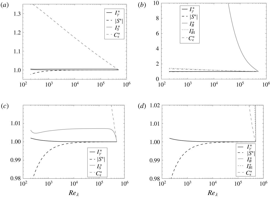
All of these quantities are supposed to be invariants for high Reynolds number free decaying HIT. Let us first analyse the case of Saffman turbulence, which is reported in figure 7(a). A zoom is provided in figure 7(c). The invariants are normalised by their asymptotic value at
 $Re_{\unicode[STIX]{x1D706}}=5\times 10^{5}$
. The coefficient exhibiting the largest variation over the investigation range is
 $C_{\unicode[STIX]{x1D716}}$
, showing a decrease of approximately 30–35 %. This variation is associated with a lack of complete turbulence equilibrium due to the time evolution of the inertial range (Bos, Shao & Bertoglio Reference Bos, Shao and Bertoglio2007). The Birkhoff–Saffman integral exhibits a much lower sensitivity to FRN effects. In particular, the evolution observed at very high Reynolds numbers is associated with minimal effects of initial conditions (see
 $n_{{\mathcal{K}}}$
in figure 3
b). However, the parameter showing the most negligible variation is the invariant
 $I_{\unicode[STIX]{x1D6FE}}$
. Figure 7(c) shows that this parameter increases by just 0.2 % over more than three decades of
 $Re_{\unicode[STIX]{x1D706}}$
. Similar considerations can be extended to the case of Batchelor turbulence, reported in figure 7(b,d). As already shown by Meldi & Sagaut (Reference Meldi and Sagaut2012) the classical Loytsianski integral is not an invariant, while the corrected integral
 $I_{B1}$
exhibits a similar evolution as
 $C_{\unicode[STIX]{x1D716}}$
. For Batchelor turbulence, the variation of
 $C_{\unicode[STIX]{x1D716}}$
is approximately 50 %, which is much larger than that for Saffman turbulence. This is associated with a stronger relaxation of the turbulence equilibrium condition. On the other hand, the Batchelor turbulence invariant
 $I_{\unicode[STIX]{x1D6FE}}$
follows the same variation as that for Saffman turbulence, suggesting this could be a true (higher-order) universal invariant, which is also the case for
 $S$
.
Evolution of turbulence invariants over the range of
 $Re_{\unicode[STIX]{x1D706}}$
investigated. Results for (a,c) Saffman turbulence and (b,d) Batchelor turbulence are shown, respectively. All quantities are normalised by their respective value at the highest
 $Re_{\unicode[STIX]{x1D706}}$
.

5 Conclusions
Numerical simulations based on a EDQNM model were carried out in freely decaying isotropic turbulence over more than three decades of the Taylor microscale Reynolds number,
 $Re_{\unicode[STIX]{x1D706}}$
(
 $200\leqslant Re_{\unicode[STIX]{x1D706}}\leqslant 5\times 10^{5}$
) in order to ascertain the effect of the Reynolds number on the skewness
 $S$
and flatness factor
 $F$
of the longitudinal velocity derivative. The choice of EDQNM is primarily based on the fact that it permits an investigation of the Reynolds number effect on statistical moments over a large range of
 $Re_{\unicode[STIX]{x1D706}}$
. Since the moments of
 $\unicode[STIX]{x2202}u/\unicode[STIX]{x2202}x$
provide a measure of small-scale intermittency, the effect of the Reynolds number on the latter is investigated in a natural fashion, starting from the Navier–Stokes equations. Further, the present approach also avoids confinement effects that may for example exist in box turbulence simulations. While
 $S$
can be calculated directly from its definition, the effect of
 $Re_{\unicode[STIX]{x1D706}}$
on
 $F$
is analysed via the analytic expression (2.4) (Djenidi et al.
Reference Djenidi, Danaila, Antonia and Tang2017b
) through dimensional arguments where it is assumed that
 $F$
can be estimated dimensionally from only
 $k$
and
 $E(k)$
in similar fashion to the behaviour that can be determined via exact transport equations for the mean energy dissipation rate
 $\overline{\unicode[STIX]{x1D716}}$
and the palinstrophy
 $G$
. Both Batchelor turbulence and Saffman turbulence are considered. The following results are found:
(i)
$S$
reaches a constant value of approximately
$-0.53$
;(ii) the first and second terms of the
$F$
-expression (2.4) become constant, indicating that
$F$
too becomes constant. This result is also qualitatively consistent with that obtained by Qian (Reference Qian1986);(iii) the constants mentioned above are reached for
$Re_{\unicode[STIX]{x1D706}}\geqslant 10^{4}$
;(iv) the EDQNM prediction (after optimising the free coefficients introduced by the dimensional arguments) of the behaviour of
$F$
at moderate
$Re_{\unicode[STIX]{x1D706}}$
is consistent with the trend observed in the data reported in the literature, see Tang et al. (Reference Tang, Antonia, Djenidi, Danaila and Zhou2018). The prediction also shows that
$F$
approaches a constant when
$Re_{\unicode[STIX]{x1D706}}\rightarrow \infty$
;(v) the EDQNM calculation of the term
$\int _{0}^{\infty }k^{\ast 4}E_{p}^{\ast }(k^{\ast })\,\text{d}k^{\ast }$
, which Tang et al. (Reference Tang, Antonia, Djenidi, Danaila and Zhou2018) identify as the upper limit for
$F$
, indicates that, as
$Re_{\unicode[STIX]{x1D706}}$
increases, this term first increases before becoming constant when
$Re_{\unicode[STIX]{x1D706}}\geqslant 10^{4}$
.





Further, a new invariant
 $I_{\unicode[STIX]{x1D6FE}}$
is defined and compared with other classical invariants reported in the literature, such as the dissipation energy coefficient
 $C_{\unicode[STIX]{x1D716}}$
, the Birkhoff–Saffman integral and the Loytsianski integral. Over more than a three decade variation in
 $Re_{\unicode[STIX]{x1D706}}$
,
 $I_{\unicode[STIX]{x1D6FE}}$
varies by approximately 0.2 % and is independent of the large-scale features (irrespective of whether Saffman or Batchelor turbulence is used). This implies that, potentially,
 $I_{\unicode[STIX]{x1D6FE}}$
is a true invariant, against which both experimental and numerical simulation results can be tested.
While the present analysis is carried out within the framework of EDQNM, the results raise some doubts regarding the anomalous behaviour usually associated with the effect of intermittency. Further, the results suggest that these effects, which are not accounted for by the EDQNM model, cannot be fully responsible for the trends observed in figure 5. Indeed, the FRN effect captured by the EDQNM results appears to be at least comparable with that derived from the Navier–Stokes equations, as reflected in the DNS and experimental data at moderate Reynolds numbers. One can argue that the absence of a model for intermittency (generally identified as the source of the Reynolds number dependence of
 $S$
and
 $F$
) in the EDQNM model supports the view that the behaviour of
 $S$
and
 $F$
observed so far for
 $Re_{\unicode[STIX]{x1D706}}\leqslant 10^{3}$
reflects a genuine FRN effect. It is important to stress that the present results do not imply a lack of intermittency. The results simply indicate that this phenomenon does not appear to control the behaviour of
 $S$
and
 $F$
for
 $Re_{\unicode[STIX]{x1D706}}\leqslant 10^{3}$
, which is the range of investigation achievable with experiments and DNS at the present time.
In conclusion, one must at least first ensure that
 $Re_{\unicode[STIX]{x1D706}}$
is large enough for the FRN effect to be negligibly small before any anomalous behaviour due to intermittency can be assessed unambiguously.