A. Synopsis

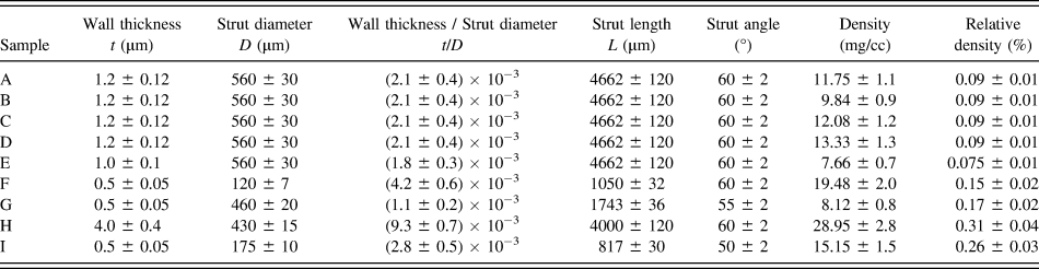
All nickel hollow microlattices were fabricated with a process developed by HRL Laboratories, LLC and discussed in the introduction [see Fig. 1(a) and Refs. Reference Schaedler, Jacobsen, Torrents, Sorensen, Lian, Greer, Valdevit and Carter22,Reference Torrents, Schaedler, Jacobsen, Carter and Valdevit25 for details]. Table I reports the geometrical parameters of all samples used in this study. The geometric parameters used to define the samples are depicted in Fig. 1(b).

TABLE I.

Summary of geometrical properties of all microlattices tested in this work.

The cyclic compressive behavior of lattices with thickness-to-diameter ratio below the critical value [Eq. (1)] is shown in Fig. 2. Four nominally identical lattices (see Table I for details) were cycled to different strain amplitudes for ∼100 cycles. A few key characteristics clearly emerge: (i) The material initially undergoes elastic deformation, which is followed by a long, fairly flat stress plateau. (ii) Upon unloading, the initial shape of the sample is almost entirely recovered. (iii) During a cycle, substantial hysteresis is observed, indicating energy dissipation (damping). (iv) The loading portion of the first cycle is substantially different from the second one, indicating irreversible fracture events; but after a few cycles of “shakedown”, the subsequent cycles quickly become self-similar, resembling the behavior of a nonlinear viscoelastic material. The energy dissipated in each cycle is attributed to a number of physical mechanisms:

1. (i) Fracture energy and plastic work. Particularly important during the first few cycles, these mechanisms are expected to largely disappear after “shakedown”.

2. (ii) Elastic buckling. When a lattice bar buckles, it dissipates strain energy, which is not recovered upon unloading.

3. (iii) Macroscale friction. When the lattice is compressed to large strains, members enter in contact with each other and dissipate energy by frictional interactions.

4. (iv) Viscous dissipation. Viscous air damping within and around the very thin hollow bars is a cause of energy loss.

5. (v) Microscale friction. Small microcracks present in the lattices dissipate energy through frictional interaction at the crack edges, even at very small applied strain.

6. (vi) Intrinsic material damping. Intrinsic damping in the constituent material contributes to energy loss.

FIG. 2.

Multicycle compression experiments on hollow metallic microlattices: results for nominally identical samples A–D (see Table I for geometric details) at different strain amplitudes. (a) Sample A under 5% strain amplitude; (b) sample B under 10% strain amplitude; (c) sample C under 25% strain amplitude; and (d) sample D under 50% strain amplitude. All samples have been cycled for ∼100 times.

This section describes an experimental protocol aimed at separating and quantifying the six mechanisms discussed above. Large-strain quasistatic cyclic compressive tests are performed to separate mechanism (i) from (ii) and (iii) and are described in Sec. II. B. Mechanisms (v) and (vi) are isolated by resonant experiments, performed at nearly zero strain (Sec. II. C). Finally, mechanism (iv) is separated by repeating all tests in air and vacuum (Sec. II. D). The observation and quantitative analyses of Sec. II. B–D are ultimately summarized in Sec. II. E.

B. Large-strain measurements

All large-strain quasistatic compression tests were performed with a servo electrical INSTRON 8862 frame and a NI SCXI data acquisition system (National Instruments, Norwood, MA). The actuator, featuring an integral concentrically mounted LVDT for precise measurement of position, moved at testing speeds of 100 mm/min to 1 μm/h and accuracy of 10 μm/s. The load was measured by a 250 g Honeywell load cell. The LabVIEW software was used to collect load and displacement data. Engineering strain and stress are defined as ε = δ/L ₀ and σ = P/A ₀ where δ is displacement measured by the LVDT and P is the load measured by external load cell. L ₀ and A ₀ represent the initial length and the cross section area, respectively. Figure 2 shows results from samples A–D (Table I) at different strain levels (5, 10, 25, and 50%). All samples were without face sheets and tested for ∼100 cycles.

Dissipated energy and damping capacity were extracted from the stress–strain data. The dissipated energy over a cycle, $\Delta U$, is by definition the area within the hysteresis loop, whereas the loss coefficient, $\Psi$, was simply obtained by normalizing $\Delta U$ with the energy under the loading curve, U, i.e., Ψ = ΔU/U.^{Reference Wong and Graesser32,Reference Lazan33}

The evolution of the dissipated energy per cycle with cycle number is plotted in Fig. 3 for different values of compressive strain amplitude. The dissipated energy monotonically decreases with cycle number for all strain amplitudes, but with a slope that is dramatically reduced after approximately 10 cycles. The difference between the initial energy dissipation and the “plateau” value expresses the contribution of irreversible mechanisms, i.e., partial nodal fractures and possible localized plastic deformation. Conversely, the “plateau” value expresses the combination of all the other mechanisms mentioned above; this energy loss is recurrent in every cycle and hence is available for damping applications. This plateau might include loss mechanisms that are related to large-strain phenomena (namely buckling-related damping) as well as microstrain phenomena (intrinsic material damping, frictional losses at crack edges, etc.). Isolating these two classes of energy loss requires performing tests at virtually zero strain, hence eliminating buckling-related modes. This was accomplished as discussed in the next section.

FIG. 3.

Dissipated energy versus cycle number for nominally identical samples A–D (see Table I for geometric details) at different strain amplitudes.

We notice that a zero-slope plateau is not exactly reached after 100 cycles, indicating continued (although much reduced) damage upon cycling. This behavior would somewhat limit the applicability of these materials for high-cycle applications. This deficiency could be addressed by an increase in the toughness of the constituent material; research in this direction is currently underway.

C. Small-strain measurements

Resonant measurements at infinitesimal strain were performed to capture intrinsic damping mechanisms, i.e., mechanisms that are not related to large deformation (or buckling) of the lattice members. All experiments were carried out with a laser Doppler vibrometer (MSA-500, Polytec GmbH, Irvine, CA). A microlattice sample was bonded to carbon-epoxy face sheets. The lower face sheet was oscillated via a piezoelectric actuator with a sinusoidal signal at a very low amplitude (∼10 nm), sweeping the frequency within the range of 0–5 kHz. The velocity of the upper plate was monitored with the Doppler vibrometer in scanning mode (to identify the modal shapes). A representative frequency response of a sample (Sample E in Table I) is shown in Fig. 4.

FIG. 4.

Extraction of the damping coefficient from the frequency response of sample E (see Table I for geometric details), captured by laser Doppler vibrometry. (a) Curve fit method; (b) half-bandwidth method.

As the mass of the face sheets is ∼10 times larger than the mass of the sample, the sandwich panel can be modeled as a discrete oscillator, with two masses connected by a spring and a damper in parallel. This simplification allows fitting of the measured frequency response on a classic oscillator model, thus allowing extraction of the damping properties of the microlattice. Incidentally, the location of the peaks provides information of the stiffness of the sample, from which the compressive Young's modulus of the microlattice can be extracted (if the density is known); this analysis is presented elsewhere.^{Reference Salari-Sharif and Valdevit34} Two different methods can be used to extract the damping coefficient of the material from the shape of the resonant peak: (i) the curve fit method, where the theoretical shape of the peak is fitted on the experimental frequency response; (ii) the half-bandwidth method, where the aspect ratio of the peak is directly correlated to the damping coefficient.

The equation of motion for the relevant mass-spring-damper can be expressed as

(2)$$\ddot x + 2{\omega _{\rm{n}}}\zeta \dot x + \omega _{\rm{n}}^2x = 2{\omega _{\rm{n}}}\zeta \dot y + \omega _{\rm{n}}^2y\quad {\rm{,}}$$

with $\zeta$ and ${\omega _{\rm{n}}}$ the damping ratio and natural frequency of the microlattice, respectively, and x and y the displacement of the two masses (face sheets). If the lower face sheet is oscillated with a harmonic sinusoidal wave, $y\left( t \right) = A{e^{i\omega t}}$, the response $x\left( t \right)$ can be written as^{Reference Meirovitch35}

(3)$$x\left( t \right) = X\left( {i\omega } \right){e^{i\omega t}}\quad {\rm{,}}$$

with

(4)$${{\left| {X\left( {i\omega } \right)} \right|} \over A} = {\left[ {{{1 + {{\left( {{{2\zeta \omega } \mathord{\left/ {\vphantom {{2\zeta \omega } {{\omega _{\rm{n}}}}}} \right. \kern-\nulldelimiterspace} {{\omega _{\rm{n}}}}}} \right)}^2}} \over {{{\left[ {1 - {{\left( {{\omega \mathord{\left/ {\vphantom {\omega {{\omega _{\rm{n}}}}}} \right. \kern-\nulldelimiterspace} {{\omega _{\rm{n}}}}}} \right)}^2}} \right]}^2} + {{\left( {{{2\zeta \omega } \mathord{\left/ {\vphantom {{2\zeta \omega } {{\omega _{\rm{n}}}}}} \right. \kern-\nulldelimiterspace} {{\omega _{\rm{n}}}}}} \right)}^2}}}} \right]^{{1 \mathord{\left/ {\vphantom {1 2}} \right. \kern-\nulldelimiterspace} 2}}}\quad {\rm{.}}$$

For method (i), Eq. (4) was fitted on the experimentally measured frequency response, and the damping ratio, $\zeta$ and natural frequency, ${\omega _{\rm{n}}}$, were extracted. The results of the fit for sample E in Table I are reported in Fig. 4(a) and the extracted damping ratio was $\zeta = 0.0328$.

Wong et al.^{Reference Wong and Graesser32} have reported that for loss factors $\eta \lt 0.28$, the half-bandwidth method (method (ii) mentioned above) is accurate enough to measure damping. In this method, the loss factor $\eta$ is extracted from the ratio of the resonant peak width (measured at an amplitude of ${1 \mathord{\left/ {\vphantom {1 {\sqrt 2 }}} \right. \kern-\nulldelimiterspace} {\sqrt 2 }}$ of the peak amplitude) to the resonance frequency.³⁶Figure 4(b) schematically demonstrates the application of the half-bandwidth method for sample E (Table I), from which a loss factor of $\eta = 0.0654$ was calculated. For small damping ($\zeta \lt 0.07$), the loss factor $\eta$ is linearly related to the damping ratio, $\zeta$ as $\eta = 2\zeta$.^{Reference Wong and Graesser32} Hence for this sample, both methods produce nearly identical results. For small damping, the loss factor is also linearly related to the loss coefficient, $\Psi$.^{Reference Wong and Graesser32} If $\Psi$ is calculated on a quarter-cycle (compressive loading–unloading), as indicated in Sec. II. B, the correlation is

(5)$$\Psi = {{4\pi \eta } \over 5}\quad {\rm{.}}$$

This correlation allows direct comparison of the results from small-strain and large-strain experiments, hence facilitating the quantitative assessment of energy loss mechanisms in ultralight microlattices. We also notice that the loss factor, η, is equal to tanδ, with δ the phase angle between stress and strain under sinusoidal loading. This notation will be used in Sec. II. E.

D. The effect of viscous dissipation

As the ultralight microlattices under consideration are made of thin hollow bars (with diameters of the order of 100 µm), the effect of viscous dissipation by air trapped in the hollow tubes and air displaced during deformation on damping might be significant. To quantify this effect, two representative samples were tested with both the large-strain (INSTRON cyclic test) and the small-strain (Doppler vibrometry) techniques, both in air and under vacuum. The vacuum chamber pressure was <5 mTorr. The results, reported in Fig. 5, indicate that the effect of viscous dissipation on damping is fairly small, even under resonant conditions (<1% for quasistatic large-strain loading and approximately 15% for the resonant test).

FIG. 5.

The effect of viscous damping. Stress–strain curves obtained for sample I in air (a) and vacuum (b), and resonant peaks obtained for sample E in air (c) and vacuum (d). See Table I for geometric details. Notice that viscous dissipation increases the damping coefficient by 1% in large-scale compression experiments, and by 15% in resonant experiments.

E. Quantitative assessment

To quantify the effect of each energy loss mechanism on the damping behavior of ultralight microlattices, it is useful to combine the results of the experiments detailed in Sec. II. B–D as indicated in Fig. 6. Although sample E (Table I) is chosen as a representative material, the behavior is qualitatively similar for all samples under investigation.

FIG. 6.

Damping capacity versus maximum compressive strain for different cycles. The damping capacity measured by resonant tests at infinitesimal strain is consistent with the compression test results at small strain amplitude. This figure allows quantitative identification of the contributions of different damping mechanisms. The dominant mechanism (Region 2) is a unique form of structural damping, largely induced by coordinated local buckling and elastic recovery of the bars upon cycling.

The damping capacity (loss coefficient) extracted from quasistatic large-strain compression tests is reported for different maximum strains (1, 2, 5, 10, 25, and 50%) and 5 cycle numbers (only 5 cycles are reported for clarity). The damping capacity extracted from the resonant tests was reported on the same plot at zero strain. In general, the damping capacity of materials is frequency dependent; as the two experiments are performed at very different frequencies (f < 0.1 Hz for the compression tests and f ∼1500 Hz for the resonant tests), there is no guarantee that the damping obtained with resonant tests would be meaningful in quasistatic situations. Notice, though, that the resonant damping capacity (∼0.16) agrees well with the damping capacity at the smallest finite strain (5%), suggesting minimal frequency dependence in this range and providing confidence in the approach. Finally, the amount of viscous damping on the resonant tests (15%, see Sec. II. D) is presented as well. Notice that the damping capacity is initially a strong function of the strain amplitude, but saturates at amplitudes ∼30%.

The combined results allow clear separation of the various energy loss mechanisms, and quantitatively express their contribution to the damping capacity of the microlattice. For each strain amplitude, four distinct regions are evident (Fig. 6): Region 1, expressing contributions of fracture and plasticity, which are not really a damping phenomenon (mechanism (i) in the classification Sec. II. A); Region 2, which displays the contribution of buckling-related and frictional damping (mechanisms (ii) and (iii)), which cannot be easily separated with this experimental protocol; Region 3, expressing the contribution of viscous damping (mechanism (iv)); and finally Region 4, expressing the contribution of intrinsic material damping phenomena (responsible at most for $\eta = 0.0006$^{Reference Lohmiller, Eberl, Schwaiger, Kraft and Balk37}) and microfriction (mechanism (v) and (vi)).

The relative importance of the 4 regions is a strong function of the strain amplitude. Region 2 (largely attributed to buckling-related damping) plays a significant role at strain amplitudes larger than 10% and becomes the dominant mechanism at strains in excess of 25%. The relative contributions do not change at amplitudes larger than ∼30%. If we discard fracture/plasticity-related energy loss, at 50% strain, for sample E, we have Region 2: 60%; Region 3: 4%; Region 4: 17%.

The dominant contribution of Region 2 justifies the modeling efforts presented in the following section, ultimately aimed at optimizing the microlattice geometry to maximize this damping mechanism.

It is instructive to compare the damping performance of the materials tested in this work with the universe of existing metallic materials. As discussed in the introduction, the conventional figure of merit for the damping performance of plates, $\Phi = E^{{1 \mathord{\left/ {\vphantom {1 3}} \right. \kern-\nulldelimiterspace} 3}} \tan {\delta \mathord{\left/ {\vphantom {\delta \rho }} \right. \kern-\nulldelimiterspace} \rho }$,^{Reference Ashby, Evans, Fleck, Gibson, Hutchinson and Wadley1} is used for comparison. For all microlattices, the loss coefficient $\Psi = {{\Delta U} \mathord{\left/ {\vphantom {{\Delta U} U}} \right. \kern-\nulldelimiterspace} U}$ is extracted from quasistatic measurements, and $\tan \delta$ is estimated from Eq. (5) (recall that η = tanδ). The Young's modulus, E, is extracted from the linear elastic portion of the stress–strain curve, and the density, $\rho$, is obtained by measuring both the weight and the volume of the samples. The envelope of all experimental results (Table I) is presented in Fig. 7 alongside the universe of metallic materials (monolithic metals, metal–matrix composites, and metallic foams). With this choice of axes, design lines (loci of uniform $\Phi$) have slope of −1. Notice that ultralight nickel microlattices are vastly superior to any metal available. It is important to emphasize, though, that the extremely low density of these samples implies that the actual amount of energy that can dissipated in each compression cycle is rather low, potentially forcing the designer to adopt unreasonably large volumes. In the next section, a simple analytical model for the dissipated energy per cycle (and for $\Phi$) will be derived and subsequently adopted in an optimization problem to identify the geometric designs that will maximize the damping performance of microlattices.

FIG. 7.

Material selection chart for vibration management of plates. All metallic materials (including metal matrix composites) are depicted, alongside the hollow metallic microlattices tested in this work (the ellipse represents the envelope of experimental results).

A. Mechanical model

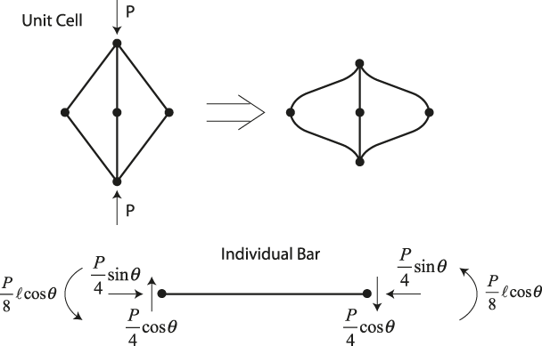
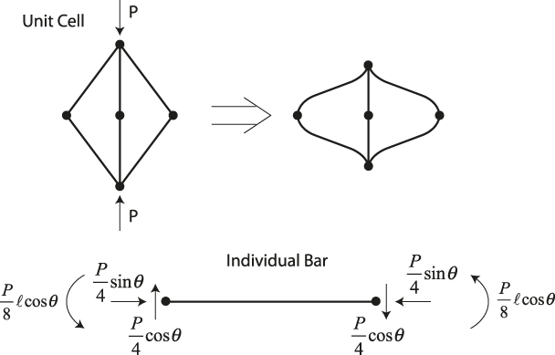
A free-body diagram for a bar within the microlattice under compression is depicted in Fig. 9. Notice that as the lattice topology is not stretching dominated, each bar experiences a combination of axial compression, bending and transverse shear. Local buckling can occur by shell compression near the clamped end (where the normal compressive stress due to bending and axial load is maximum, see Fig. 8(a)) or by shell shear (throughout the beam length). Because the shear stress is nearly zero where the normal stress is maximum (and vice versa), the two mechanisms are not heavily coupled. The implication – verified by FE simulations as explained below – is that the buckling load of the cylinder can be estimated as the minimum between the shell compression and the shell shear critical loads. Expressing the axial load and the moment on the bar as a function of the compressive load applied on one unit cell, P, the maximum normal compressive stress in the bar can be written as

(6)$${\sigma _{{\rm{max}}}} = {{P\ell \cos \theta } \over {2\pi t{D^2}}} + {{P\sin \theta } \over {4\pi tD}}\quad {\rm{,}}$$

where t, D, $\ell$, and θ are the thickness, diameter, length, and inclination of the lattice bar, respectively [Fig. 1(b)]. The bar will buckle by shell compression when the maximum stress in the bar equals the critical local buckling stress. According to classic buckling theory,^{Reference Calladine41} local buckling in a cylindrical shell of circular cross section under combinations of axial compression and bending occurs when the normal stress on the compressive side of the shell reaches the critical stress for axisymmetric (compression-only) buckling i.e.,

(7)$${\sigma _{{\rm{cr}}}} = {{2Et} \over {D\sqrt {3\left( {1 - {\nu ^2}} \right)} }}\quad {\rm{,}}$$

with E and $\nu$ are the Young's modulus and Poisson's ratio of the material. For the nickel microlattice under consideration, $E = 210\;GPa$ and $\nu = 0.3$, respectively. By equating Eqs. (6) and (7), the buckling strength of the bar under compression-bending (equal to ¼ of the strength of the unit cell) can be expressed as

(8)$$P_{{\rm{cr,bar}}}^{{\rm{b + c}}} = {{{P^{{\rm b+c}}_{{\rm{cr}}}}} \over 4} = {{2\pi E{t^2}} \over {\sqrt {3\left( {1 - {\nu ^2}} \right)} \left( {\sin \theta + {{2\ell \cos \theta } \over D}} \right)}}\quad {\rm{.}}$$

FIG. 9.

Schematic of the deformation of a unit cell of the lattice under external compression, and free-body diagram of a single bar. Note that each bar experiences a combination of axial compression, bending and shear loads.

The critical stress for shear buckling in a cylinder of circular cross-section can be estimated analytically as^{Reference Teng and Rotter42}

(9)$${\tau _{{\rm{cr}}}} = 1.5E\sqrt {{{\sqrt {{{Dt} \mathord{\left/ {\vphantom {{Dt} 2}} \right. \kern-\nulldelimiterspace} 2}} } \over \ell }} {t \over D}\quad {\rm{.}}$$

Shear buckling occurs when the maximum shear stress in a single bar (given by ${{P\cos \theta } \mathord{\left/ {\vphantom {{P\cos \theta } {\left( {2\pi Dt} \right)}}} \right. \kern-\nulldelimiterspace} {\left( {2\pi Dt} \right)}}$) equals the critical stress, which leads to

(10)$$P_{{\rm{cr,bar}}}^{{\rm{sh}}} = {{P_{{\rm{cr}}}^{{\rm{sh}}}} \over 4} = {{3\pi E{t^2}} \over {4\cos \theta }}\sqrt {{{\sqrt {{{Dt} \mathord{\left/ {\vphantom {{Dt} 2}} \right. \kern-\nulldelimiterspace} 2}} } \over \ell }} \quad {\rm{.}}$$

The ratio between the shell shear and the shell compression buckling loads will then scale as

(11)$${{P_{{\rm{cr}}}^{{\rm{sh}}}} \over {P_{{\rm{cr}}}^{{\rm{b + c}}}}}\sim{\left( {{\ell \over D}} \right)^{{1 \mathord{\left/ {\vphantom {1 2}} \right. \kern-\nulldelimiterspace} 2}}}{\left( {{t \over D}} \right)^{{1 \mathord{\left/ {\vphantom {1 4}} \right. \kern-\nulldelimiterspace} 4}}}\quad {\rm{.}}$$

As ${\ell \mathord{\left/ {\vphantom {\ell D}} \right. \kern-\nulldelimiterspace} D}$ and ${t \mathord{\left/ {\vphantom {t D}} \right. \kern-\nulldelimiterspace} D}$ increase, shell compression buckling becomes the dominant failure mechanism. Although Eqs. (8) and (10) predict comparable buckling loads for all samples in Table I, numerical buckling analyses (eigenvalue extractions) performed with ABAQUS on single cantilever bars clamped at one end and subjected to an inclined load at the other end reveal that Eq. (8) is very accurate while Eq. (10) is too conservative. The implication is that all samples under investigation fail by local shell compression buckling, at a critical load that is very well captured by Eq. (8). This is in agreement with visual observations during the compression experiments. To verify that shear buckling is also inconsequential for all optimal geometries presented in Sec. III. B, numerical buckling analyses (eigenvalue extraction) were performed on a number of samples, with three conclusions: (i) for ${\ell \mathord{\left/ {\vphantom {\ell D}} \right. \kern-\nulldelimiterspace} D} > 4$, buckling occurs by shell compression for ${t \mathord{\left/ {\vphantom {t D}} \right. \kern-\nulldelimiterspace} D} > 0.0025$; (ii) for ${\ell \mathord{\left/ {\vphantom {\ell D}} \right. \kern-\nulldelimiterspace} D} > 8$, buckling occurs by shell compression for ${t \mathord{\left/ {\vphantom {t D}} \right. \kern-\nulldelimiterspace} D} > 0.001$; (iii) in all cases, the critical loads are in good agreement with Eq. (8). As all optimal designs satisfy the geometric conditions (i) or (ii) (see Sec. III.B), shear buckling is never a concern, and will henceforth be neglected.

An energy method is used to calculate the stiffness of bar. Upon global compression, the elastic energy stored in the entire unit cell is the sum of axial, shear, and bending contributions (the shear term is the smallest, but not always insignificant):

(12)$$U = {{{P^2}{{\cos }^2}\theta {\ell ^3}} \over {6E\pi {D^3}t}} + {{{P^2}{{\sin }^2}\theta \ell } \over {4E\pi Dt}} + {{{P^2}{{\cos }^2}\theta \ell } \over {2G\pi Dt}}\quad {\rm{,}}$$

with G the shear modulus of the material $\left( {G = {E \mathord{\left/ {\vphantom {E {\left( {2\left( {1 + \nu } \right)} \right)}}} \right. \kern-\nulldelimiterspace} {\left( {2\left( {1 + \nu } \right)} \right)}} = 81\;{\rm{GPa}}} \right)$.

The unit cell stiffness can be defined as $K = {P \mathord{\left/ {\vphantom {P \delta }} \right. \kern-\nulldelimiterspace} \delta }$, with $\delta$ the vertical displacement of the unit cell. The strain energy in the unit cell can be related to the displacement by $U = {1 \over 2}P\delta$. By imposing that this equation be equal to Eq. (12), the stiffness of each bar can be calculated as

(13)$${K_{{\rm{bar}}}} = {K \over 2} = {{3\pi Et{D^3}} \over {2{\ell ^3}{{\cos }^2}\theta }}{1 \over {\left[ {1 + {3 \over 2}{{\tan }^2}\theta {{\left( {{D \over \ell }} \right)}^2} + 6{{\left( {{D \over \ell }} \right)}^2}\left( {1 + \nu } \right)} \right]}}\quad {\rm{.}}$$

Assuming that the entire elastic energy is dissipated upon buckling (a slight overestimation, as noted in Fig. 8), the energy loss from each bar can be expressed as

(14)$$\Delta {E_{{\rm{bar}}}} = {1 \over 2}{{P_{{\rm{cr,bar}}}^2} \over {{K_{{\rm{bar}}}}}}\quad {\rm{.}}$$

To calculate the energy dissipation of the whole lattice, the number of bars that buckle at any given applied compressive strain must be evaluated. Assuming an infinite lattice experiencing layer-by-layer deformation, and assuming that each bar folds onto itself upon buckling (so that the compress cell has a thickness equal to 2D), the fraction of bars, f, that needs to buckle to accommodate the global lattice strain is given by

(15)$$f = {{{\varepsilon _{{\rm{max}}}}} \over {1 - {D \mathord{\left/ {\vphantom {D {\left( {\ell \sin \theta } \right)}}} \right. \kern-\nulldelimiterspace} {\left( {\ell \sin \theta } \right)}}}}\quad {\rm{.}}$$

The number of bars in the whole lattice is given by ${N_{\rm{b}}} = 16{n_x}{n_y}{n_z}$, where ${n_x}$, ${n_y}$, and ${n_z}$ are the number of unit cells in X, Y, and Z directions, respectively.

The dimensions of the lattice are related to the dimensions of the unit cell by $L = 2\ell \cos \theta {n_y}$, $H = 2\ell \sin \theta {n_z}$, and $W = 2\ell \cos \theta {n_x}$.

Finally, from a simple energy balance, the energy dissipation in the bulk structure is extracted as

(16)$$\Delta U = {{f\,{N_{\rm{b}}}\Delta {E_{{\rm{bar}}}}} \over {W\,L\,H}} = {{2f\Delta {E_{{\rm{bar}}}}} \over {{\ell ^3}\sin \theta \,{{\cos }^2}\theta }}\quad {\rm{.}}$$

The continuum approximation underlying Eq. (15) is expected to be reliable for samples containing a large number of unit cells. As all samples available for characterization in this work contained at most 3 unit cells [defined as depicted in Fig. 1(b)], experimental verification of Eq. (16) presents some challenges. These challenges are exacerbated by the presence of manufacturing imperfections in most samples. To address these difficulties, and verify the reliability of the model, the following analysis was performed.

Figure 10 shows the dissipated energy per cycle after 100 cycles for four nominally identical samples (samples A–D in Table I) tested at different strain amplitudes. The red markers represent experimental measurements, while the three lines are model predictions. The solid line is a plot of Eq. (16), for the nominal dimensions of the sample. Notice that the model significantly underpredicts the dissipated energy. This discrepancy is attributed to (i) finite size effects and (ii) manufacturing imperfections, and justified as follows. The dashed staircase curve represents predictions of the energy dissipated for each full layer collapse (one layer equals ½ unit cell), with the strains for layer collapse based on experimental observation (0 collapsed layers observed at 5% strain, 1 at 10% strain, 2 at 25% strain, and 3 at 50% strain). This line represents the discrete version of Eq. (16) for a 2-unit cell sample. Finally, the dash-dot curve corrects for manufacturing imperfections, by estimating the dissipated energy per layer on the actual (counted) number of bars in each layer for the specific test samples (rather than calculating the number of unit cells based on measured overall sample sizes and unit cell nominal dimensions). Notice that the dash-dot curve is in very good agreement with the experimental measurements for all values of compressive strain amplitude.

FIG. 10.

Dissipated energy in each cycle for samples A–D (the samples are nominally identical, see Table I for details) after 100 cycles, as a function of the maximum compressive strain applied in each cycle. The red markers represent experimental results, whereas the solid line depicts the analytical prediction from Eq. (16). The dashed line corrects the analytical model for a sample with only 4 unit cells across the thickness, based on visual observation of layer-by-layer buckling. The dash-dot line incorporates measured geometric imperfections in the samples.

To verify the model-experiment agreement for other sample geometries and relative densities, four different samples (samples D–G in Table I) were tested at 50% compressive strain amplitude for ∼100 cycles. The results are reported in Fig. 11. Notice that the simple analytical model [Eq. (16)] can capture the dissipated energy per cycle quite accurately (with a discrepancy of ∼13–45%, depending on sample geometry).

FIG. 11.

Dissipated energy in each cycle for samples D–G after 100 cycles. The black square markers represent experimental results, whereas the red circular markers depict the analytical prediction from Eq. (16).

It is worth emphasizing that the mechanical models presented in this section assume that the lattice response (both in terms of stiffness and strength, including the nonlinear postbuckling behavior) is fully represented by the response of a single unit cell (or even a single bar). A number of recent studies have clearly indicated that this is not necessarily the case^{Reference Arabnejad and Pasini16,Reference Vigliotti, Deshpande and Pasini18} : this is particularly important for the buckling behavior, where different lattice topologies require multicell representative volume elements (RVE) of different dimensions to accurately capture the infinite lattice response.^{Reference Vigliotti, Deshpande and Pasini18} A recent study showed that the situation is even more complex for hollow lattices dominated by local shell buckling, where details of the boundary conditions on the sides of the RVE have a dramatic effect; in some cases, single bar models can overpredict the buckling strength of a lattice by 2–5X.^{Reference Valdevit, Godfrey, Schaedler, Jacobsen and Carter26} Similar trends were observed for stiffness predictions, where the overprediction can be even more dramatic.^{Reference Godfrey and Valdevit27} Efforts are currently underway to develop an improved procedure for accurate numerical calculation of local buckling and yielding strength of infinite hollow lattices (S. W. Godfrey and L. Valdevit, unpublished results), but are beyond the scope of this work. We emphasize that the goal of the analytical model contained in this article is to provide an order-of-magnitude estimate for the energy loss in loading–unloading cycles on ultralight hollow lattices. The fact that simple (albeit somewhat inaccurate) models can capture the order of magnitude of the energy loss is used to (i) support the claim that structural damping is in large part due to local kinking of the bars and (ii) extrapolate the best damping performance that can be expected from this kind of materials (see Sec. III. B). These simple analytical models are not meant to be used for accurate prediction of the mechanical response of these lattices. More detailed analytical and/or computational models are certainly needed for that goal.

B. Trends for optimal design

The mechanical model described in Sec. III. A can be used to explore the parameter space and identify optimal designs. Two optimization problems will be addressed: the maximization of the energy dissipated per cycle, $\Delta U$, and the maximization of the damping figure of merit, $\Phi = E^{{1 \mathord{\left/ {\vphantom {1 3}} \right. \kern-\nulldelimiterspace} 3}} \tan {\delta \mathord{\left/ {\vphantom {\delta \rho }} \right. \kern-\nulldelimiterspace} \rho }$.

1. Maximization of dissipated energy per cycle, $\Delta U$

Expressed in nondimensional form, the geometric parameters of the system are the truss angle, $\theta$; the bar aspect ratio, ${D \mathord{\left/ {\vphantom {D \ell }} \right. \kern-\nulldelimiterspace} \ell }$; and the cross-section aspect ratio, ${t \mathord{\left/ {\vphantom {t D}} \right. \kern-\nulldelimiterspace} D}$.

The objective function (to be maximized) can be expressed as

(17)$$\Delta U = {{8\pi f\,E{{\left( {{t \mathord{\left/ {\vphantom {t D}} \right. \kern-\nulldelimiterspace} D}} \right)}^3}} \over {9\left( {1 - {\nu ^2}} \right)\sin \theta }}{{\left[ {1 + {{3{{\tan }^2}\theta {{\left( {{D \mathord{\left/ {\vphantom {D \ell }} \right. \kern-\nulldelimiterspace} \ell }} \right)}^2}} \mathord{\left/ {\vphantom {{3{{\tan }^2}\theta {{\left( {{D \mathord{\left/ {\vphantom {D \ell }} \right. \kern-\nulldelimiterspace} \ell }} \right)}^2}} 2}} \right. \kern-\nulldelimiterspace} 2} + 6\left( {1 + \nu } \right){{\left( {{D \mathord{\left/ {\vphantom {D \ell }} \right. \kern-\nulldelimiterspace} \ell }} \right)}^2}} \right]} \over {{{\left( {\sin \theta + {{2\cos \theta } \mathord{\left/ {\vphantom {{2\cos \theta } {\left( {{D \mathord{\left/ {\vphantom {D \ell }} \right. \kern-\nulldelimiterspace} \ell }} \right)}}} \right. \kern-\nulldelimiterspace} {\left( {{D \mathord{\left/ {\vphantom {D \ell }} \right. \kern-\nulldelimiterspace} \ell }} \right)}}} \right)}^2}}}\quad {\rm{.}}$$

The range of the geometric parameters is dictated by manufacturing constraints, beam theory limitations, and the recoverability condition [Eq. (1)], and can be expressed as follows:

(18)$$\eqalign{ &#x0026; {10^{ - 5}} \lt {t \mathord{\left/ {\vphantom {t D}} \right. \kern-\nulldelimiterspace} D} \lt {\left( {{t \mathord{\left/ {\vphantom {t D}} \right. \kern-\nulldelimiterspace} D}} \right)_{{\rm{cr}}}} \cr &#x0026; 2 \lt {L \mathord{\left/ {\vphantom {L D}} \right. \kern-\nulldelimiterspace} D} \lt 16 \cr &#x0026; {D \mathord{\left/ {\vphantom {D \ell }} \right. \kern-\nulldelimiterspace} \ell } \lt 0.25 \cr &#x0026; 45^\circ \lt \theta \lt 75^\circ \quad {\rm{,}} \cr}$$

where L is the cell size [$L = 2\ell \cos \theta$, see Fig. 1(b)], and $\left( {{t \mathord{\left/ {\vphantom {t D}} \right. \kern-\nulldelimiterspace} D}} \right)_{{\rm{cr}}}$ is given by Eq. (1). (To be consistent with a layer-by-layer deformation model [implicit in Eq. (15)], Eq. (1) is modified by assuming ${\varepsilon _{{\rm{max}}}} = 50\%$ regardless of the actual values of ${\varepsilon _{{\rm{max}}}}$. This is a conservative choice based on the observation that each layer deforms by ∼50% before the next layer starts buckling).

The relative density of the samples is calculated from simple hollow truss geometry^{Reference Valdevit, Jacobsen, Greer and Carter11}:

(19)$$\bar \rho = {{2\pi } \over {{{\cos }^2}\theta \sin \theta }}{\left( {{D \over \ell }} \right)^2}{t \over D}\quad {\rm{.}}$$

The relative density is swept in the range of 0.01–2%, and for each density the constrained optimization problem described above is solved with the “fmincon” algorithm in MATLAB.

The energy loss versus the relative density of the material for different compressive strain amplitudes is depicted in Fig. 12(a), with optimal dimensions in Figs. 12(b)–12(d). Importantly, and conveniently, the optimal lattice geometry is independent of the maximum compressive strain, whereas obviously the dissipated energy is monotonic in the maximum strain amplitude.

FIG. 12.

(a) Maximum achievable energy loss for nickel microlattices as a function of relative density for different compressive strain amplitudes. (b–d) Optimal lattice dimensions.

Initially, ${t \mathord{\left/ {\vphantom {t D}} \right. \kern-\nulldelimiterspace} D}$ increases rapidly with relative density, with the angle constant at its upper bound (75°) and ${D \mathord{\left/ {\vphantom {D \ell }} \right. \kern-\nulldelimiterspace} \ell }$ constant at its lower bound (0.032). The dissipated energy is increasing very fast with the relative density. Very soon, the ${t \mathord{\left/ {\vphantom {t D}} \right. \kern-\nulldelimiterspace} D} \lt \left( {{t \mathord{\left/ {\vphantom {t D}} \right. \kern-\nulldelimiterspace} D}} \right)_{{\rm{cr}}}$ constraint becomes active, at which point a further increase in ${t \mathord{\left/ {\vphantom {t D}} \right. \kern-\nulldelimiterspace} D}$ (and hence the energy) is only possible with a steep decrease in angle and an increase in ${D \mathord{\left/ {\vphantom {D \ell }} \right. \kern-\nulldelimiterspace} \ell }$. When the angle reaches its lower bound (45°), ${t \mathord{\left/ {\vphantom {t D}} \right. \kern-\nulldelimiterspace} D}$ reaches a plateau and the density can only increase by further increasing ${D \mathord{\left/ {\vphantom {D \ell }} \right. \kern-\nulldelimiterspace} \ell }$; in this density range, the dissipated energy still increases with density, but at a much lower rate. Finally, at a relative density of 0.75%, ${D \mathord{\left/ {\vphantom {D \ell }} \right. \kern-\nulldelimiterspace} \ell }$ reaches its upper bound (0.25), at which point a further increase in density requires a drop in ${t \mathord{\left/ {\vphantom {t D}} \right. \kern-\nulldelimiterspace} D}$ and an increase in angle; the dissipated energy first drops quickly, and then starts increasing again at a very low rate. The peak in dissipated energy occurs at the relative density of 0.75%, for all applied strain levels.

Figure 13(a) compares the energy dissipation of the existing samples strained to 50% amplitude (samples D–H (Table I)) with the optimal designs. As all experimentally characterized samples have $\theta = 60^\circ$ (Table I), the optimal results for this constant angle are reported as well. According to the optimization results, for a relative density of 0.17%, the maximum energy loss at 50% strain would be 1293 J/m³, which is ∼26 times larger than the model predictions for sample G (Table I), which has the same density but different geometries. Conversely, notice that the energy dissipation for sample F (∼456 J/m³), at a relative density of 0.15%, is very close to the prediction for optimal 60° lattices at that density (511 J/m³). A comparison of the actual and optimal geometries reveals a striking similarity (Table II), confirming the validity of the analytical model and the optimization process.

FIG. 13.

(a) Dissipated energy for a number of samples (D–H) of different relative densities (experimental results versus analytical model), compared with the energy that could be dissipated by optimally designed lattices (for the blue line, the lattice member angle is treated as a variable, whereas for the green line, the angle is fixed at 60°). (b) Calculated relative density versus wall thickness over truss diameter for samples D–H (see Table I for details). The dotted red line represents the transition between recoverable and unrecoverable behavior. This confirms that the poor agreement between theory and model for sample H ($\bar \rho = 0.3\%$) is due to the fact that the sample was not designed to withstand a 50% compressive strain (see stress–strain curve in the inset, confirming lack of recoverability).

TABLE II.

Comparison of the geometries of sample F and the optimal lattice for a relative density of 0.15%.

Notice that the analytical model cannot capture the experimental results for sample H (Table I), at a relative density of 0.31%, and that the prediction for sample H largely exceeds the optimal results at that relative density. This discrepancy is easily explained looking at the dimensions of sample H: the cross-section aspect ratio $\left( {{t \mathord{\left/ {\vphantom {t D}} \right. \kern-\nulldelimiterspace} D}} \right)$ of this sample exceeds the critical value for recoverability [Eq. (1)] [see Fig. 13(b)]. The inset in the figure confirms that sample H does not undergo elastic recovery from a strain of 50%. Once again, these observations reinforce confidence in the model.

Collectively, the optimization results indicate that an energy dissipation per cycle as large as 9000 J/m³ is theoretically possible from a nickel microlattice with $\theta = 45^\circ$, ${D \mathord{\left/ {\vphantom {D \ell }} \right. \kern-\nulldelimiterspace} \ell } = 0.25$, and ${t \mathord{\left/ {\vphantom {t D}} \right. \kern-\nulldelimiterspace} D} = 0.007$, compressed to a strain amplitude of 50%. This value is ∼20 higher than the largest energy dissipation measured to date. However, an increase in dissipation energy does not necessarily guarantee an increase in damping. The next section addresses the optimization of the damping figure of merit, $\Phi = E^{{1 \mathord{\left/ {\vphantom {1 3}} \right. \kern-\nulldelimiterspace} 3}} \tan {\delta \mathord{\left/ {\vphantom {\delta \rho }} \right. \kern-\nulldelimiterspace} \rho }$.

2. Maximization of damping figure of merit, $\Phi$

Analytical prediction of the damping figure of merit requires reasonable estimates of relative density, Young's modulus, and $\tan \delta$. It is well known that analytical models overpredict (often dramatically) both stiffness and strength of hollow microlattices.^{Reference Valdevit, Godfrey, Schaedler, Jacobsen and Carter26,Reference Godfrey and Valdevit27} In this case, the challenge is exacerbated by the substantial structural damage that ultralight samples receive upon large amplitude straining (see Fig. 2). A crude analytical model will be attempted nonetheless and used to optimize $\Phi$. The goal is a prediction of the trends of the optimal $\Phi$ with relative density (and information on the optimal designs), rather than a reliable prediction of $\Phi$ itself.

As suggested in Refs. Reference Kalathur and Lakes39,Reference Dong and Lakes43, $\tan \delta$ for a nonlinear dissipating material can be estimated by the shape of the stress–strain curve of a linear viscoelastic material with the same stress and strain amplitudes, ${\sigma _{{\rm{max}}}}$ and ${\varepsilon _{{\rm{max}}}}$. The area under the compressive portion of the stress–strain curve (Lissajous figure) for a linear material can be expressed as $W_{\rm{d}} = \left( {{{2\pi } \mathord{\left/ {\vphantom {{2\pi } 5}} \right. \kern-\nulldelimiterspace} 5}} \right)\sigma _{{\rm{max}}} \varepsilon _{{\rm{max}}}$. By equating this area to the dissipated energy in a cycle, i.e., ${W_{\rm{d}}} = \Delta U$, and taking ${\sigma _{{\rm{max}}}}$ as the buckling strength of the lattice, given by^{Reference Valdevit, Godfrey, Schaedler, Jacobsen and Carter26}

(20)$${\sigma _{{\rm{max}}}} = {{2\pi {E_{\rm{s}}}\left( {{D \mathord{\left/ {\vphantom {D \ell }} \right. \kern-\nulldelimiterspace} \ell }} \right){{\left( {{t \mathord{\left/ {\vphantom {t \ell }} \right. \kern-\nulldelimiterspace} \ell }} \right)}^2}} \over {{{\cos }^3}\theta \sqrt {3\left( {1 - {\nu ^2}} \right)} \left( {1 + \left( {{D \mathord{\left/ {\vphantom {D \ell }} \right. \kern-\nulldelimiterspace} \ell }} \right)\tan {\theta \mathord{\left/ {\vphantom {\theta 2}} \right. \kern-\nulldelimiterspace} 2}} \right)}}\quad {\rm{,}}$$

an estimate for $\tan \delta$ can be obtained.

As Eq. (20) overpredicts the buckling strength even at the first cycle, and the lattice strength is greatly reduced after the first cycle (Fig. 2), the resulting estimate for $\tan \delta$ results grossly conservative.

The Young's modulus of the lattice, $E = {\sigma \mathord{\left/ {\vphantom {\sigma \varepsilon }} \right. \kern-\nulldelimiterspace} \varepsilon }$, can be estimated analytically by normalizing the unit cell stiffness expression [Eq. (10)]. As $\sigma = {P \mathord{\left/ {\vphantom {P {\left( {2\ell ^2 \cos ^2 \theta } \right)}}} \right. \kern-\nulldelimiterspace} {\left( {2\ell ^2 \cos ^2 \theta } \right)}}$, $\varepsilon = {\delta \mathord{\left/ {\vphantom {\delta {\left( {2\ell \sin \theta } \right)}}} \right. \kern-\nulldelimiterspace} {\left( {2\ell \sin \theta } \right)}}$, and $K = {P \mathord{\left/ {\vphantom {P \delta }} \right. \kern-\nulldelimiterspace} \delta }$, where K is the unit cell stiffness given by Eq. (13), we obtain

(21)$$E = {{3\pi {E_{\rm{s}}}\sin \theta {{\left( {{D \mathord{\left/ {\vphantom {D \ell }} \right. \kern-\nulldelimiterspace} \ell }} \right)}^3}\left( {{t \mathord{\left/ {\vphantom {t \ell }} \right. \kern-\nulldelimiterspace} \ell }} \right)} \over {{{\cos }^4}\theta }}{1 \over {1 + {3 \over 2}{{\left( {{D \over \ell }} \right)}^2}{{\tan }^2}\theta + 6\left( {1 + \nu } \right){{\left( {{D \over \ell }} \right)}^2}}}\quad {\rm{.}}$$

As ultralight hollow microlattices immediately buckle upon compression, this estimate dramatically overpredicts the stiffness measured by the slope of the stress–strain curve under quasistatic loading.^{Reference Godfrey and Valdevit27} Recently, it was shown that the agreement is much improved if the stiffness is measured in noncontact methods, e.g., by laser Doppler vibrometry.^{Reference Salari-Sharif and Valdevit34} At any rate, the use of Eq. (18) somewhat offsets the overconservative estimate of $\tan \delta$ discussed above.

For all samples, the relative density is calculated from the geometric parameters in Table II using Eq. (19).

To get a sense of the possible error in using this model to estimate $\Phi$, Table III compares density, stiffness, strength, energy dissipation, and damping figure of merit extracted from the experiments and the analytical models. As expected, the model consistently overestimates stiffness, density, and strength, while slightly underestimating the energy dissipation. Clearly the actual value of the figure of merit is not a reliable number, and tends to underestimate the experimental results by a factor of 5–30. However, the trends of $\Phi$ with relative density are expected to be reliable.

TABLE III.

Mechanical properties of different samples cyclically loaded to 50% strain.

The damping figure of merit, $\Phi = E^{{1 \mathord{\left/ {\vphantom {1 3}} \right. \kern-\nulldelimiterspace} 3}} \tan {\delta \mathord{\left/ {\vphantom {\delta \rho }} \right. \kern-\nulldelimiterspace} \rho }$, was maximized under the same geometrical and physical constraints adopted in Sec. II. B. 1 [Eq. (18)]. Figure 14 shows the optimal damping figure of merit as a function of relative density. Notice that the results are independent on the compressive strain amplitudes, with all the curves collapsing on a master curve. Interestingly, the optimal geometrical parameters are identical to those for optimal energy dissipation (Fig. 12).

FIG. 14.

Damping figure of merit for optimal designs, as a function of relative density. The result is independent on the strain amplitude. Note that the damping performance of buckling-dominated hollow metallic microlattices rapidly drops when the lattice density is increased above ∼0.1%.

The damping performance $\Phi$ increases very fast with increasing relative density (by increasing ${D \mathord{\left/ {\vphantom {D \ell }} \right. \kern-\nulldelimiterspace} \ell }$ and ${t \mathord{\left/ {\vphantom {t D}} \right. \kern-\nulldelimiterspace} D}$), until the angle reaches its minimum value and ${t \mathord{\left/ {\vphantom {t D}} \right. \kern-\nulldelimiterspace} D}$ saturates to 0.007 (equal to $\left( {{t \mathord{\left/ {\vphantom {t D}} \right. \kern-\nulldelimiterspace} D}} \right)_{{\rm{cr}}}$ for $\theta = 45^\circ$), at a relative density, $\bar \rho \sim 0.1\%$. Beyond this point, the angle maintains its minimum value, ${t \mathord{\left/ {\vphantom {t D}} \right. \kern-\nulldelimiterspace} D}$ remains at the critical value, and ${D \mathord{\left/ {\vphantom {D \ell }} \right. \kern-\nulldelimiterspace} \ell }$ increases, as discussed above; this results in a dramatic decrease in $\Phi$ with further increase in relative density (the drop occurs even as the dissipated energy continues to increase, see Fig. 14). At a relative density, $\bar \rho \sim 0.75\%$, ${D \mathord{\left/ {\vphantom {D \ell }} \right. \kern-\nulldelimiterspace} \ell }$ reaches its upper bound, after which further increase in density requires an increase in the angle and a decrease in ${t \mathord{\left/ {\vphantom {t D}} \right. \kern-\nulldelimiterspace} D}$; this results in a second sudden drop in the damping figure of merit $\Phi$. Eventually, $\Phi$ reaches a plateau, after which it continues to decrease very slowly.

The results clearly show that the damping performance peaks at very low relative density (∼0.1%) and dramatically decreases as the density is increased. This confirms that the exceptional buckling-related damping of these novel material systems is limited to the ultralight regime. If higher relative densities are required (for examples, to meet stiffness and/or strength constraints), additional damping mechanisms should be introduced. One possibility is the fabrication of multilayer hollow microlattices, where one layer possesses significant intrinsic damping.