2 The numerical database

The numerical simulation of turbulent flow in square ducts in the incompressible limit is a much more challenging task for numerical algorithms than the canonical cases of plane channel and pipe flow. The main reason resides in the availability of only one direction of space inhomogeneity, which prevents the use of efficient inversion procedures for Poisson equations based on double trigonometric expansions (Kim & Moin Reference Kim and Moin1985; Orlandi Reference Orlandi2012). Although this difficulty can be circumvented through use of two-dimensional Poisson solvers based on cyclic reduction (Gavrilakis Reference Gavrilakis1992), similar efficiency can also be achieved with compressible algorithms made to operate at low Mach number (Modesti & Pirozzoli Reference Modesti and Pirozzoli2017), thus avoiding the solution of a discrete Poisson equation; however, at the expense of stiffness in the allowed time step for explicit integration of acoustic waves. In the present work we use a fourth-order co-located finite-difference solver, previously used for DNS of compressible turbulence, also in the low-Mach-number regime (Pirozzoli & Bernardini Reference Pirozzoli and Bernardini2013; Modesti & Pirozzoli Reference Modesti and Pirozzoli2016). Here, the convective terms in the Navier–Stokes equations are preliminarily expanded to quasi-skew-symmetric form, in such a way as to discretely preserve total kinetic energy from convection (Pirozzoli Reference Pirozzoli2010). Semi-implicit time stepping is used for time advancement in order to relax the acoustic time step limitation, thus allowing efficient operation at low Mach number, also through use of the entropy evolution equation rather than the total energy equation. The streamwise momentum equation is forced in such a way as to maintain a constant mass flow rate (the spatially uniform driving term is hereafter referred to as $\unicode[STIX]{x1D6F1}$ , see (4.1)), periodicity is exploited in the streamwise direction, and isothermal no-slip boundary conditions are used at the channel walls.

Table 1.

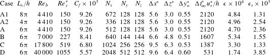
Flow parameters for DNS of square duct flow. $L_{x}$ is the streamwise length of the computational domain, with $2h$ the duct side length. $Re_{b}=2hu_{b}/\unicode[STIX]{x1D708}$ is the bulk Reynolds number, and $Re_{\unicode[STIX]{x1D70F}}^{\ast }=hu_{\unicode[STIX]{x1D70F}}^{\ast }/\unicode[STIX]{x1D708}$ is the friction Reynolds number. $\unicode[STIX]{x0394}x$ is the mesh spacing in the streamwise direction, and $\unicode[STIX]{x0394}z$ , $\unicode[STIX]{x0394}y_{w}$ are the maximum and minimum mesh spacings in the cross-stream direction, all given in global wall units, $\unicode[STIX]{x1D6FF}_{v}^{\ast }=\unicode[STIX]{x1D708}/u_{\unicode[STIX]{x1D70F}}^{\ast }$ . $\unicode[STIX]{x0394}t_{av}^{\ast }$ is the effective averaging time interval, and the convergence indices $\unicode[STIX]{x1D716}$ and $\unicode[STIX]{x1D716}_{s}$ are defined in (2.2)–(2.3).

Let $h$ be half of the duct side length, the DNS have been carried out for a duct with $[-h:h]\times [-h:h]$ cross-section, and whose length is $6\unicode[STIX]{x03C0}h$ , the latter selected on the basis of preliminary box size sensitivity studies (see table 1) as well as conclusions of previous authors (Gavrilakis Reference Gavrilakis1992). Four DNS have been carried out at bulk Mach number $M_{b}=u_{b}/c_{w}=0.2$ (where $c_{w}$ is the speed of sound at the wall temperature) and bulk Reynolds number $Re_{b}=4000{-}40000$ (see table 1) – hereafter labelled with letters from A to D. Two additional simulations have been carried out at the same flow conditions as case A, in a longer (A1) and shorter (A2) computational domain, in order to quantify the effect of the box size on the flow statistics. The turbulence Mach number $M_{t}=u^{\prime }/c_{w}$ nowhere exceeds $0.01$ for any of the simulations and hence the present DNS may be regarded as a close approximation of genuinely incompressible turbulence. For the sake of later reference, we will use the $+$ superscript to denote quantities made non-dimensional with respect to the local wall friction, namely with $u_{\unicode[STIX]{x1D70F}}=(\unicode[STIX]{x1D70F}_{w}/\unicode[STIX]{x1D70C}_{w})^{1/2}$ , $\unicode[STIX]{x1D6FF}_{v}=\unicode[STIX]{x1D708}/u_{\unicode[STIX]{x1D70F}}$ , and the $\ast$ superscript to denote quantities made non-dimensional with respect to the perimeter-averaged friction, $\unicode[STIX]{x1D70F}_{w}^{\ast }=h\overline{\unicode[STIX]{x1D6F1}}/2$ , $u_{\unicode[STIX]{x1D70F}}^{\ast }=(\unicode[STIX]{x1D70F}_{w}^{\ast }/\unicode[STIX]{x1D70C}_{w})^{1/2}$ , $\unicode[STIX]{x1D6FF}_{v}^{\ast }=\unicode[STIX]{x1D708}/u_{\unicode[STIX]{x1D70F}}^{\ast }$ . The velocity field is initialized with the incompressible laminar solution (Shah & London Reference Shah and London1978), with a superposed array of longitudinal rollers,

where $A=0.01u_{b}$ , and additional random disturbances, to achieve fast transition to a turbulent state. Streamwise-averaged flow statistics have been collected at uniform time intervals, and processed off-line to control independence on the initial conditions and statistical convergence.

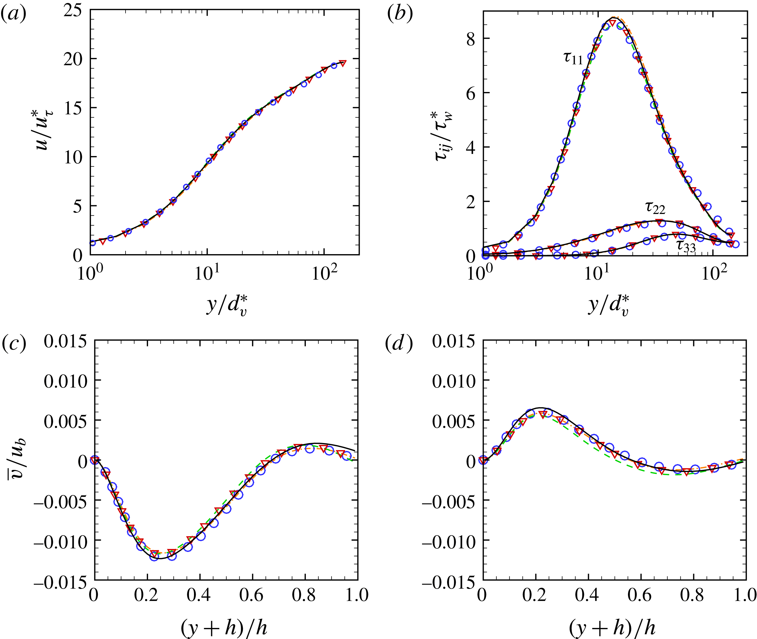
A comparison of the results obtained for flow case A with previous DNS is shown figure 1, which supports good agreement of the mean velocities and velocity fluctuation statistics. The effect of the box dimension on the flow statistics is also found to be marginal, also recalling that Pinelli et al. (Reference Pinelli, Uhlmann, Sekimoto and Kawahara2010) used $L_{x}=4\unicode[STIX]{x03C0}h$ , and Vinuesa et al. (Reference Vinuesa, Noorani, Lozano-Durán, Khoury, Schlatter, Fischer and Nagib2014) used $L_{x}=8\unicode[STIX]{x03C0}h$ .

Figure 1.

Profiles of mean velocity (a) and turbulent normal stresses (b) along the wall bisector, and cross-stream velocity at $z/h=-0.75$ (c), $z/h=-0.25$ (d), for flow case A (solid lines), A1 (dashed), A2 (dash-dot), Pinelli et al. (Reference Pinelli, Uhlmann, Sekimoto and Kawahara2010) (triangles), Vinuesa et al. (Reference Vinuesa, Noorani, Lozano-Durán, Khoury, Schlatter, Fischer and Nagib2014) (circles).

Statistical convergence of DNS is a crucial issue, and as pointed out by Oliver et al. (Reference Oliver, Malaya, Ulerich and Moser2014), the statistical error may be even dominant over the numerical error. In this respect, previous DNS of duct flow highlighted the need of extremely long averaging time intervals to achieve statistical convergence, typically several times longer than in plane channel flow. This issue is mainly associated with the weakness of secondary motions. Vinuesa et al. (Reference Vinuesa, Prus, Schlatter and Nagib2016) introduced a convergence indicator for duct flow based on a mean momentum balance check (see (4.1)), similar to what is usually done for plane channel flow, in which linearity of the total stress is taken as an index of statistical convergence. Specifically, those authors considered the root mean square of the residual of (4.1) expressed in wall units (say $R^{\ast }$ ) and averaged over the wall bisector,

We have also considered an additional convergence indicator based on deviations of the computed statistical properties from the expected geometrical symmetry, which we define as

where $\overline{u}_{Q}$ denotes the mean velocity averaged over the four quadrants.

Following Vinuesa et al. (Reference Vinuesa, Prus, Schlatter and Nagib2016), in order to account for the effect of the streamwise length of the computational domain on statistical convergence, we consider effective time averaging intervals, $\unicode[STIX]{x0394}t_{av}^{\ast }=\unicode[STIX]{x0394}t_{av}L_{x}/(6h)$ , expressed in eddy-turnover times, $h/u_{\unicode[STIX]{x1D70F}}^{\ast }$ . For the sake of reference, previous studies used $\unicode[STIX]{x0394}t_{av}^{\ast }=52h/u_{\unicode[STIX]{x1D70F}}^{\ast }$ (Gavrilakis Reference Gavrilakis1992), $\unicode[STIX]{x0394}t_{av}^{\ast }=1136h/u_{\unicode[STIX]{x1D70F}}^{\ast }$ (Pinelli et al. Reference Pinelli, Uhlmann, Sekimoto and Kawahara2010), $\unicode[STIX]{x0394}t_{av}^{\ast }=1662h/u_{\unicode[STIX]{x1D70F}}^{\ast }$ (Vinuesa et al. Reference Vinuesa, Noorani, Lozano-Durán, Khoury, Schlatter, Fischer and Nagib2014). The statistical convergence parameters are given in table 1 for all DNS. The mean momentum balance convergence indicator is found to be much less than $10^{-3}$ for all simulations, which is the threshold proposed by Vinuesa et al. (Reference Vinuesa, Noorani, Lozano-Durán, Khoury, Schlatter, Fischer and Nagib2014). The symmetry indicator further suggests that distortions of $\overline{u}$ with respect to a four-fold symmetric state are much less than $1\,\%$ . For comparison, we find the symmetry indicator to be $\unicode[STIX]{x1D716}_{s}=3.75\times 10^{-3}$ for the DNS of Pinelli et al. 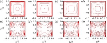(Reference Pinelli, Uhlmann, Sekimoto and Kawahara2010), and $\unicode[STIX]{x1D716}_{s}=2.05\times 10^{-3}$ for Vinuesa et al. (Reference Vinuesa, Noorani, Lozano-Durán, Khoury, Schlatter, Fischer and Nagib2014). Further information regarding the symmetry of the statistical distributions is provided in figure 2, where we compare contours of $\overline{u}$ and $\overline{v}$ with their distribution averaged over the four quadrants. Deviations from statistical symmetry are generally small, but more significant for the secondary motion, which is slower to converge, and for flow case D, as also quantified by the $\unicode[STIX]{x1D716}_{s}$ indicator. Given this caveat, and consistent with the previous literature, the statistical distributions in cross-stream planes are hereafter reported in terms of their average over the four duct quadrants.

Figure 2.

Comparison of contours of $\overline{u}$ (a–d) and $\overline{v}$ (e–h) with the same distributions averaged over quadrants $\overline{u}_{Q}$ , $\overline{v}_{Q}$ (thick lines). (a,e) Case A, (b,f) Case B, (c,g) Case C, (d,f) Case D. Contour levels are shown for $0\leqslant \overline{u}/u_{b}\leqslant 1.3$ , in intervals of $0.1$ , and $-0.02\leqslant \overline{v}/u_{b}\leqslant 0.02$ , in intervals of $0.0025$ . Dashed lines denote negative values.

Figure 3.

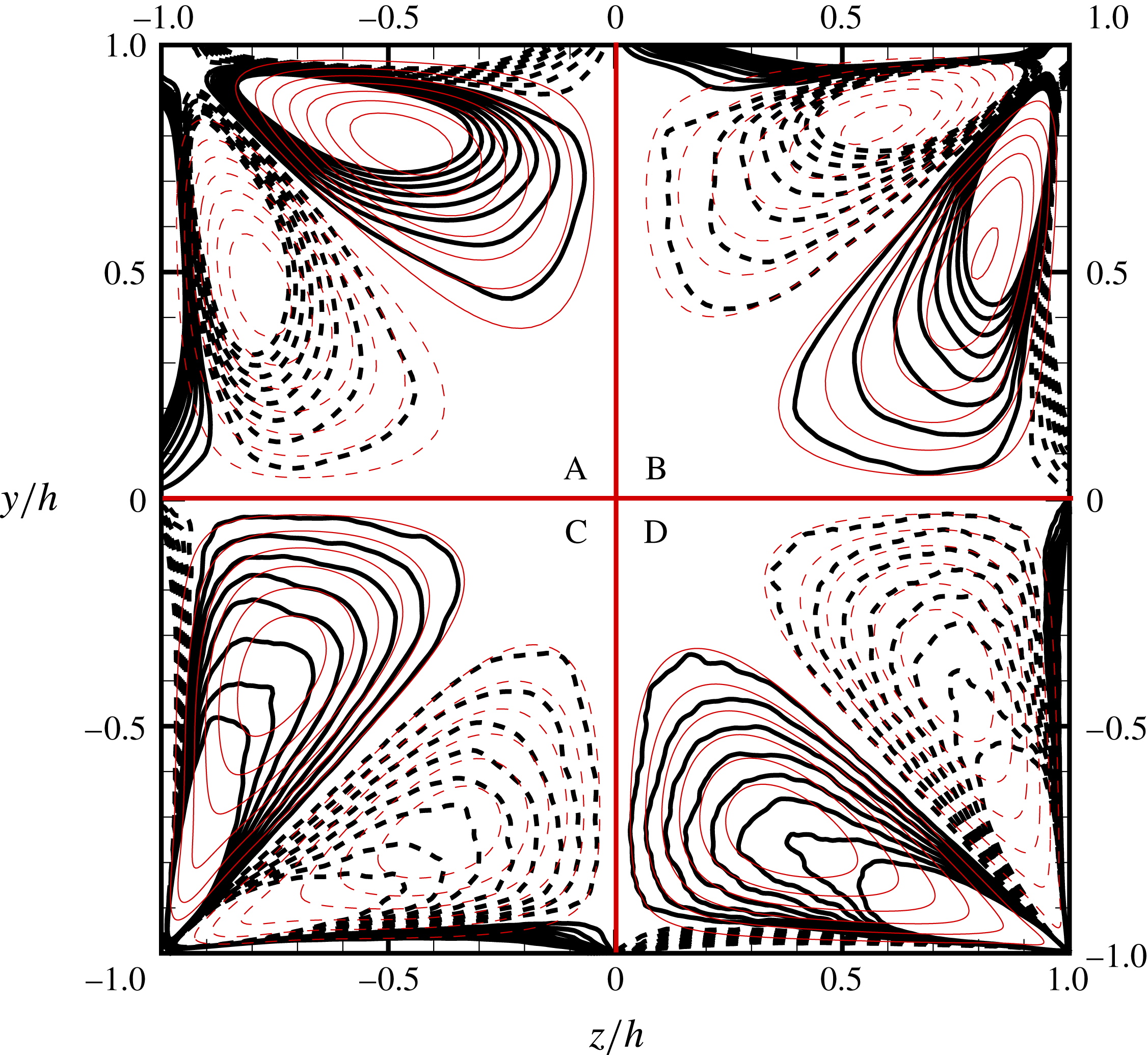
Vorticity contours (black lines) and mean cross-flow streamlines (red lines) for flow cases A (top left), B (top right), C (bottom left) and D (bottom right). Contours are shown for $\unicode[STIX]{x1D713}/(hu_{b})$ (thin lines) and $\overline{\unicode[STIX]{x1D714}}_{x}/(k^{2}hu_{b})$ (thick lines) are shown from $-0.0024$ to $0.0024$ , in intervals of $3\times 10^{-4}$ , with $k^{2}=49.373/h^{2}$ (see § 5). Dashed lines denote negative values.

3 The secondary motions

A visual representation of the structure of the secondary motions is provided in figure 3, where we show the mean streamwise vorticity ( $\overline{\unicode[STIX]{x1D714}}_{x}=\unicode[STIX]{x2202}\overline{v}/\unicode[STIX]{x2202}z-\unicode[STIX]{x2202}\overline{w}/\unicode[STIX]{x2202}y$ ) and the corresponding streamfunction $\unicode[STIX]{x1D713}$ , evaluated by solving

As well established (Brundrett & Baines Reference Brundrett and Baines1964), the time-averaged secondary motions consist of eight eddies with triangular shape and obvious symmetry properties, whose primary effect is to redistribute momentum excess from the channel core towards the duct corners, where momentum is less than the average because of the concurrent friction exerted by the two adjacent walls. The outer scaling ( $u_{b}$ , $h$ ) used in figure 3 suggests that the intensity of the eddies is approximately unaffected by Reynolds number variations. The validity of $u_{b}$ as a velocity scale for the secondary motions as opposed to other options, e.g. the friction velocity $u_{\unicode[STIX]{x1D70F}}^{\ast }$ , is supported by the analysis of several flow statistics, some of which are reported in the following. This conclusion is probably inconsistent with recent theoretical analysis predicting $u_{\unicode[STIX]{x1D70F}}$ as the correct scale for the secondary motions in the asymptotic high- $Re$ limit (Spalart, Garbaruk & Stabnikov Reference Spalart, Garbaruk and Stabnikov2018); however, the discrepancy may be well due to the relatively limited range of Reynolds numbers attainable with DNS. Although the streamline topology does not change with $Re$ , it appears that the geometry of the eddies does in fact change in two ways. First, the vortex centres exhibit a non-monotonic shift from the corners with the Reynolds number in a way to be discussed in detail later on. Second, the streamlines penetrate deeper into the corners as $Re$ increases. As also pointed out by Pinelli et al. (Reference Pinelli, Uhlmann, Sekimoto and Kawahara2010), the vorticity distribution is more complex than the streamline pattern. At low Reynolds number (A) a primary negative vorticity patch is observed in the duct core, which is accompanied by a mirror layer of positive vorticity signed near the wall, that forms as a result of the no-slip condition (Orlandi Reference Orlandi1990). As the Reynolds number increases, the main negative vorticity peak becomes stronger in amplitude, and it becomes progressively confined towards the duct corner, whereas the weaker core vorticity remains roughly of constant strength. A secondary negative vorticity peak eventually emerges, which is visible in (D) at approximately the same position as the centres of the cross-stream eddies. Hence, it appears that the strongest vorticity (hereafter referred to as corner vorticity) becomes progressively disconnected with the streamfunction distribution, whereas the core vorticity, which scales well in outer units ( $u_{b}/h$ ), becomes closely associated with the streamfunction at high enough  $Re$ .

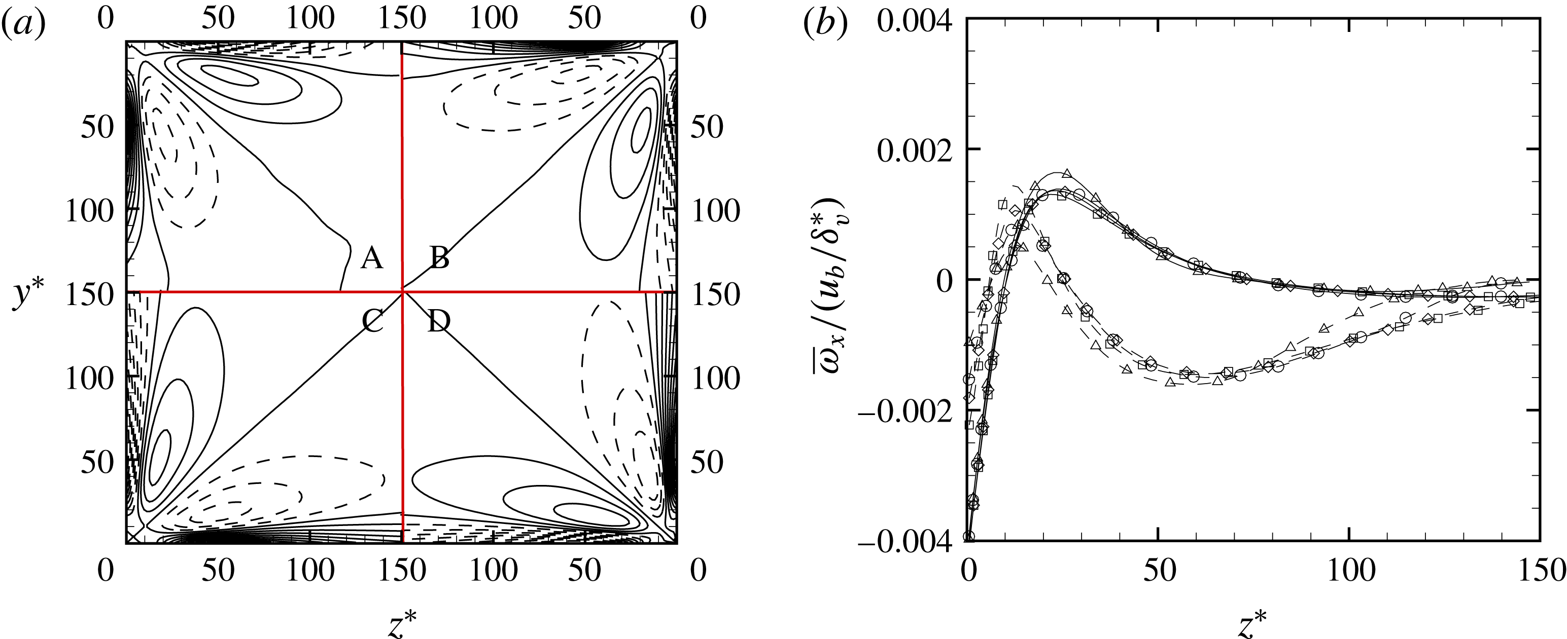
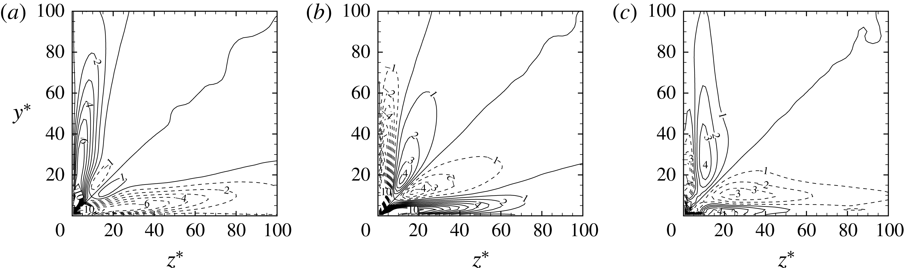
The structure and scaling of the corner vorticity is analysed in detail in figure 4, where data are reported as a function of the inner-scaled distance from the duct walls. As noted in previous studies, the strongest vorticity tends to be concentrated around the corner bisector and at the wall. Based on the DNS dataset we find empirically that the corner vorticity scales well across the Reynolds number range in mixed units ( $u_{b},\unicode[STIX]{x1D6FF}_{v}^{\ast }$ ). Hence, the associated motions become progressively confined to the duct corners as $Re$ increases, and their intensity increases when expressed in outer units, as seen in figure 3. Despite its greater strength, this wall-confined vorticity does not contribute significantly to the secondary motions at high $Re$ . This is easily understood, since the total circulation associated with the core vorticity is expected to scale as $u_{b}h$ , whereas the contribution of the corner vorticity is expected to scale as $u_{b}\unicode[STIX]{x1D6FF}_{v}^{\ast }$ , hence decreasing as $Re_{\unicode[STIX]{x1D70F}}^{\ast }$ with respect to the former. This expectation is supported from the DNS data, which also shows that the ratio of the secondary circulation to the primary circulation is approximately $0.42$ , irrespective of the Reynolds numbers. A separate analysis (not reported here) further shows that the streamline pattern away from corners is not significantly altered in shape and intensity if the corner vorticity is removed from the right-hand side of (3.1).

Figure 4.

(a) Contours of streamwise vorticity near the duct corner in inner coordinates, $z^{\ast }=(z+h)/\unicode[STIX]{x1D6FF}_{v}^{\ast }$ , $y^{\ast }=(y+h)/\unicode[STIX]{x1D6FF}_{v}^{\ast }$ . Contours are shown for $-0.004\leqslant \overline{\unicode[STIX]{x1D714}}_{x}/(u_{b}/\unicode[STIX]{x1D6FF}_{v}^{\ast })\leqslant 0.004$ , in intervals of $0.0005$ (dashed lines denote negative values). (b) Vorticity profiles at $y^{\ast }=25$ (dashed lines) and $y^{\ast }=75$ (solid lines) for flow case A (triangles), B (circles), C (diamonds), D (squares).

Figure 5.

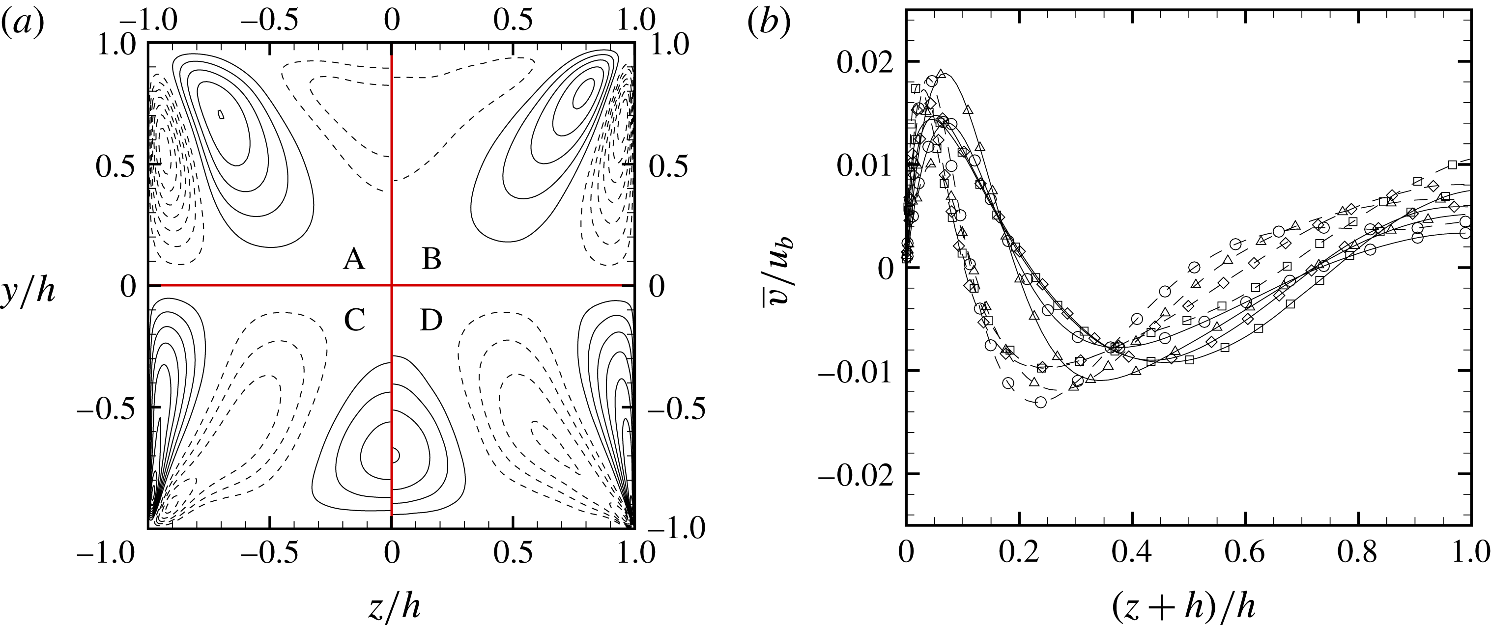
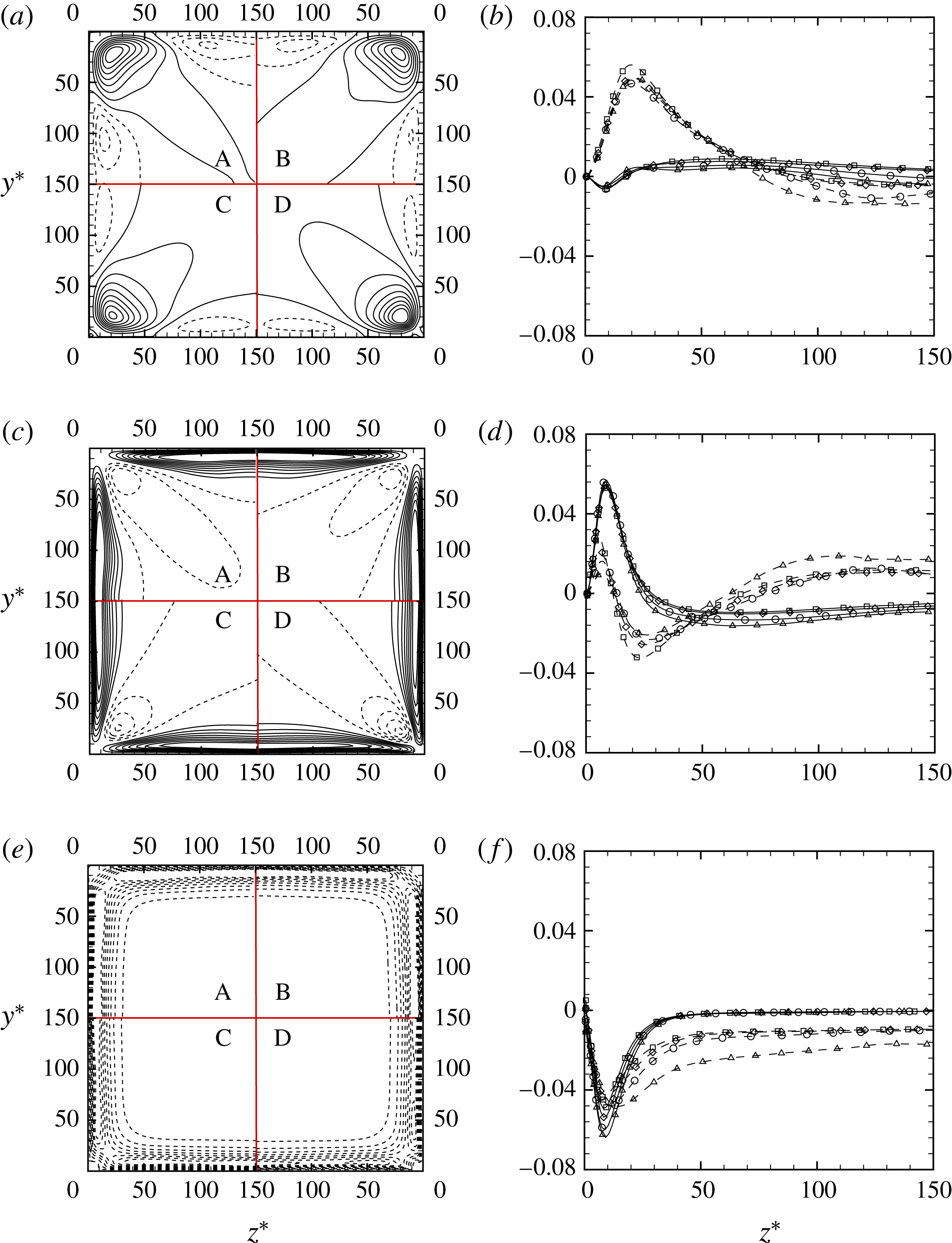
(a) Contours of mean cross-stream velocity component $\overline{v}$ . Contour levels are shown for $-0.02\leqslant \overline{v}/u_{b}\leqslant 0.02$ , in intervals of $0.0025$ (dashed lines denote negative values), flow cases reported as A (top left), B (top right), C (bottom left), D (bottom right). (b)  $\overline{v}$ profiles at $y/h=-0.75$ (dashed lines) and $y/h=-0.5$ (solid lines) for flow case A (triangles), B (circles), C (diamonds), D (squares).

Figure 6.

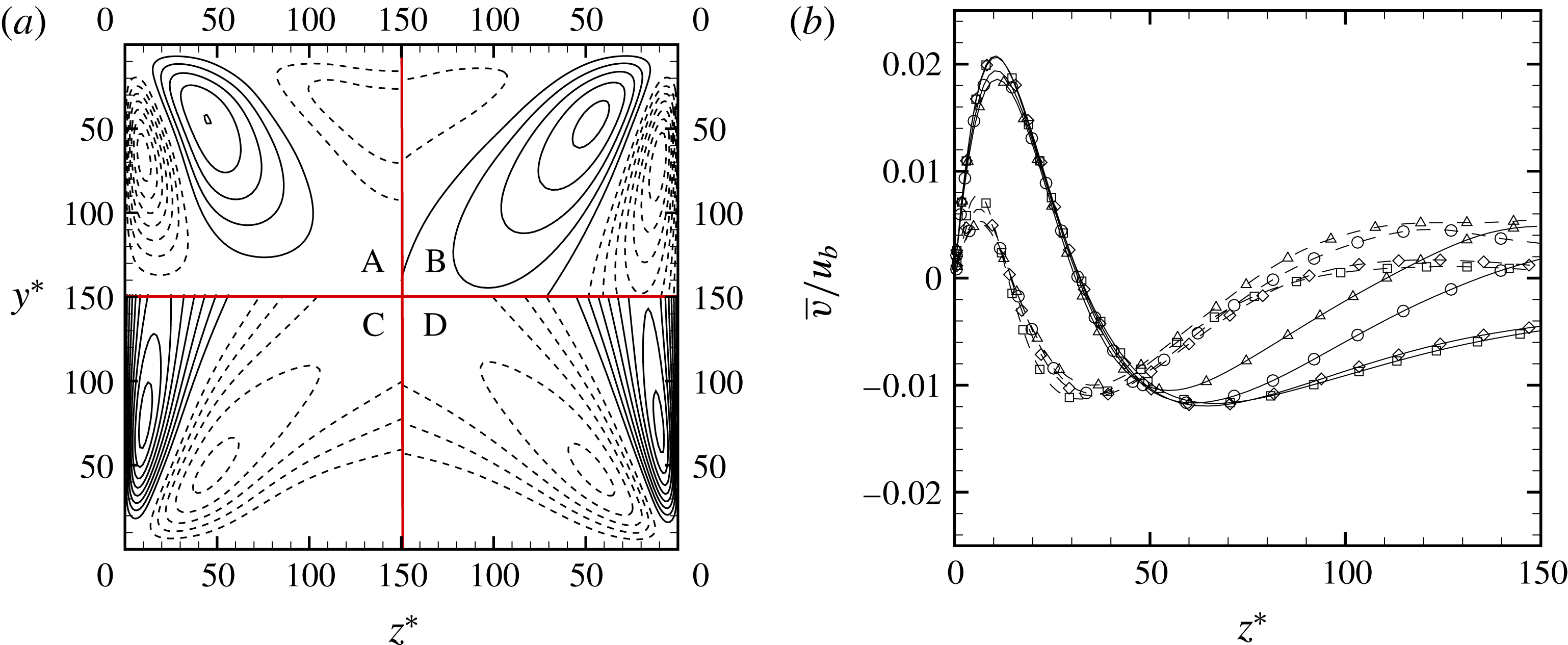
(a) Contours of mean cross-stream velocity component $\overline{v}$ near the duct corner in inner coordinates, $z^{\ast }=(z+h)/\unicode[STIX]{x1D6FF}_{v}^{\ast }$ , $y^{\ast }=(y+h)/\unicode[STIX]{x1D6FF}_{v}^{\ast }$ . Contour levels are shown for $-0.02\leqslant \overline{v}/u_{b}\leqslant 0.02$ , in intervals of $0.0025$ (dashed lines denote negative values). (b)  $\overline{v}$ profiles at $y^{\ast }=25$ (dashed lines) and $y^{\ast }=75$ (solid lines) for flow case A (triangles), B (circles), C (diamonds), D (squares).

Consistent with the previous observations, figure 5 confirms that, at least in the Reynolds number range under scrutiny, the velocity associated with the secondary motions scales well with $u_{b}$ , with a maximum intensity of approximately $2\,\%u_{b}$ . Relative maxima are attained for the vertical velocity component along the corner bisector traced to the momentum inflow towards the duct corners, and parallel to the left sidewall and along the wall bisector, as a consequence of the return motions to guarantee continuity. The observed scaling of the corner vorticity can then be explained as a viscous effect, associated with retardation of the secondary stream scaling on $O(u_{b})$ , and occurring over a distance proportional to the viscous length scale $\unicode[STIX]{x1D6FF}_{v}^{\ast }$ , thus yielding the observed trend $\overline{\unicode[STIX]{x1D714}}_{x}\sim u_{b}u_{\unicode[STIX]{x1D70F}}^{\ast }/\unicode[STIX]{x1D708}$ . An alternative scaling may be considered by assuming that the length scale in the duct corners is $\unicode[STIX]{x1D708}/u_{b}$ , which would then lead to $\overline{\unicode[STIX]{x1D714}}_{x}\sim u_{b}^{2}/\unicode[STIX]{x1D708}$ . The difference between the two scalings is difficult to judge based on the available data; however, we are slightly in favour of the former. Figure 5 also confirms that at sufficiently high $Re$ a new maximum of $v$ becomes isolated within the duct corners, which is associated with the corner vorticity. As clarified in figure 6, the intensity of these motions also scales with $u_{b}$ , and it is geometrically similar (although on a smaller scale) to the core secondary flow. An interesting scenario thus emerges, which includes two concurrent contributions to the secondary motions: (i) a core circulation, with typical velocity $u_{b}$ and typical length scale $h$ ; (ii) a corner circulation with typical velocity still $u_{b}$ and typical length scale likely to be $\unicode[STIX]{x1D6FF}_{v}^{\ast }$ . At low Reynolds number the two circulations basically coincide, whereas at higher Reynolds number the latter becomes progressively segregated to the duct corners, and the core circulation emerges in the bulk flow.

Figure 7.

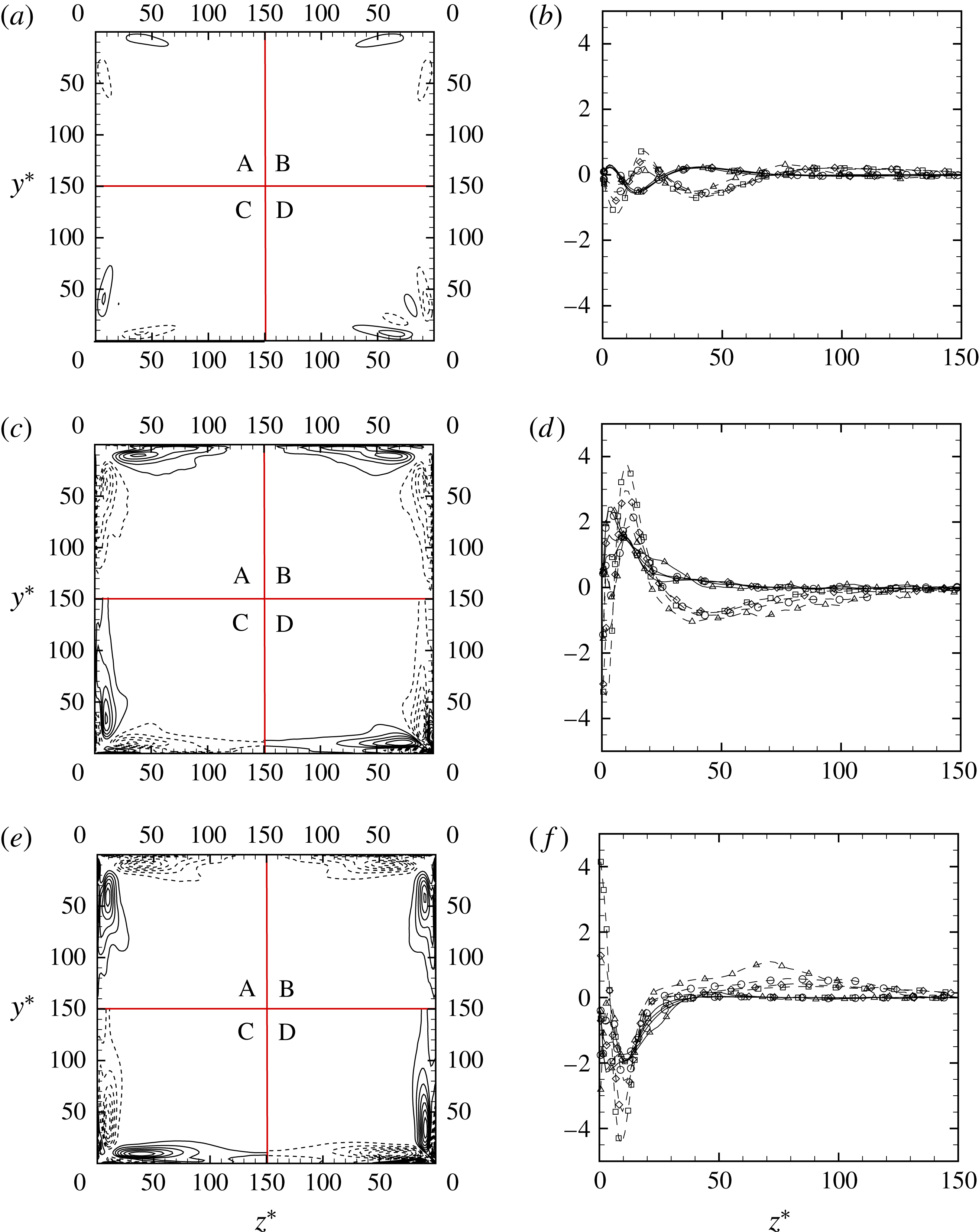
Terms in the mean streamwise vorticity budget equation (3.2) near the duct corners: mean convection (a,b), turbulence (c,d), viscous diffusion (e,f). (a,c,e) Contour levels for $-5\leqslant (\cdot )/(u_{b}/\unicode[STIX]{x1D6FF}_{v}^{\ast })^{2}\times 10^{6}\leqslant 5$ , in intervals of $0.625$ (dashed lines denote negative values). (b,d,f) Profiles of the budget terms at $y^{\ast }=25$ (dashed lines) and $y^{\ast }=75$ (solid lines) for flow case A (triangles), B (circles), C (diamonds), D (squares).

Deeper insight into the nature of the secondary motions can be gained from the mean streamwise vorticity equation (Einstein & Li Reference Einstein and Li1958)

The various terms which appear in (3.2) are associated with the effect of mean cross-stream convection (left-hand side), secondary turbulent shear stress (first term on right-hand side), normal stress anisotropy (second term), and viscous diffusion (third term). Their distributions as determined from DNS are shown in figure 7, where the two turbulence terms are merged together, and all terms are normalized with respect to $(u_{b}/\unicode[STIX]{x1D6FF}_{v}^{\ast })^{2}$ – which, based on the previous discussion, is the expected order of magnitude for the time derivative of $\overline{\unicode[STIX]{x1D714}}_{x}$ . Also note that the distributions are only shown near the corners, where the various terms are sensibly different from zero. The figure supports the alleged scaling of the various terms across the given Reynolds number range. Furthermore, it is indicative of a leading balance between the turbulence terms (which are regarded as production terms in the common interpretation) and viscous diffusion, whereas it appears that convection does not yield a significant contribution to the streamwise vorticity dynamics. This scenario is consistent with low- $Re$ DNS studies (Gavrilakis Reference Gavrilakis1992), but it contradicts the typical conclusions of experimental studies, in which, however, the estimation of high-order statistics such as those occurring in (3.2) may be affected by substantial uncertainties (Demuren & Rodi Reference Demuren and Rodi1984).

More detailed information on the individual contribution of the anisotropy and the secondary shear stress terms is given in figure 8. It is found that the two terms are overall of the same order of magnitude, although only the former is generally considered in attempts of turbulence closure (Demuren & Rodi Reference Demuren and Rodi1984). Detailed inspection of the figure shows that their spatial organization is similar, but they tend to be locally opposite in sign, with strong cancellation near the walls, where both terms assume individually very large values. Comparing with their algebraic sum (repeated in panel c for convenience), it appears that non-zero values of turbulence production are primarily associated with large values of the secondary shear stress term. It is noteworthy that Nagata et al. (Reference Nagata, Hunt, Sakai and Wong2011) found that in shear-free corner flows the derivatives of the normal stresses are predominant in producing the secondary flow near the corner. This qualitative difference probably points to the importance of the mean shear in sustaining secondary motions in ducts.

Figure 8.

Turbulence terms in the mean streamwise vorticity budget equation (3.2) for flow case D: anisotropy term (a), secondary shear stress term (b), and their sum (c). Contour levels are shown for $-10\leqslant (\cdot )/(u_{b}/\unicode[STIX]{x1D6FF}_{v}^{\ast })^{2}\times 10^{6}\leqslant 10$ , in intervals of $0.5$ (dashed lines denote negative values).

4 Effect on the mean streamwise velocity field

Figure 9.

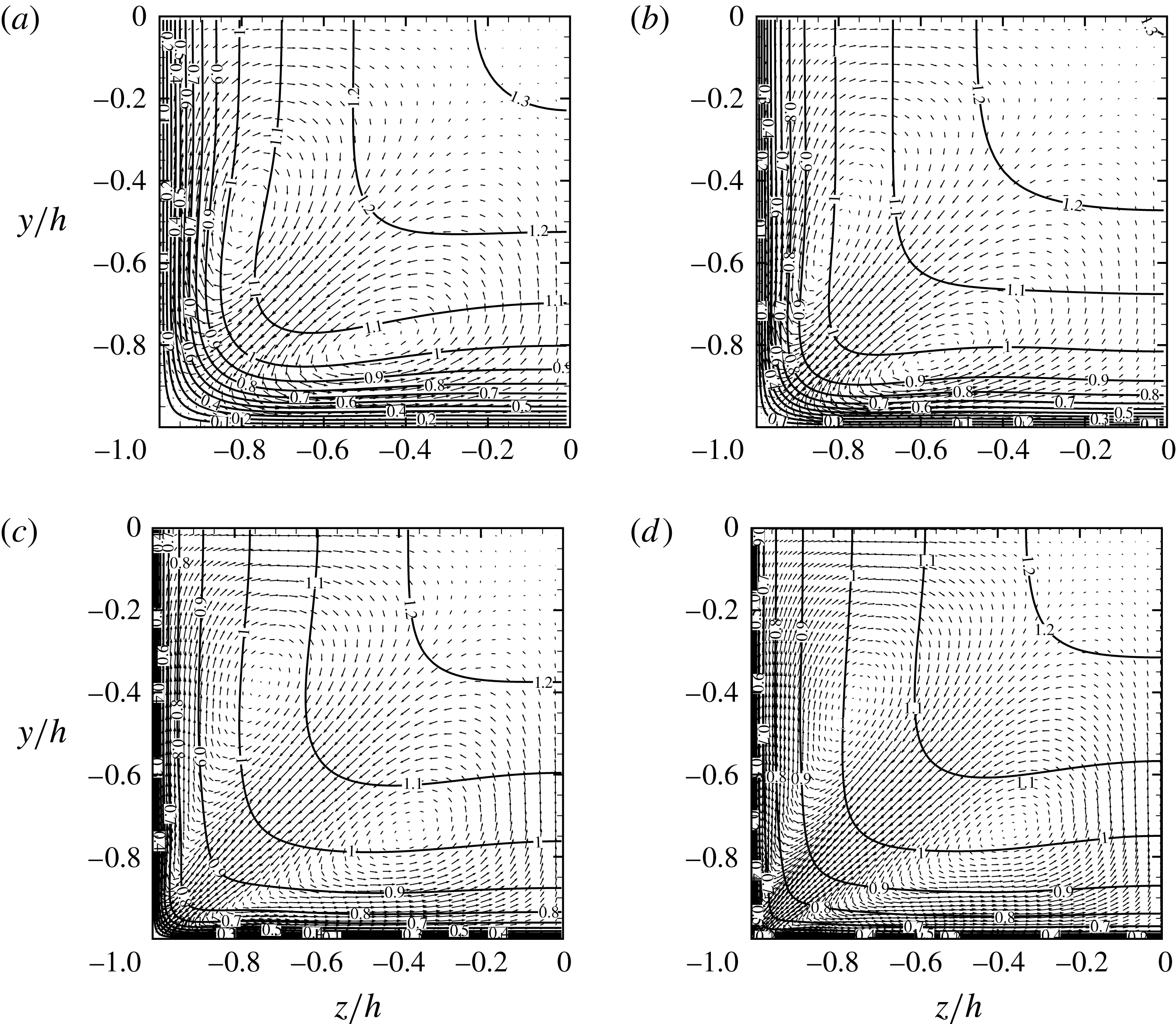
Mean streamwise velocity contours ( $0\leqslant \overline{u}/u_{b}\leqslant 1.3$ , in intervals of $0.1$ ) with superposed mean cross-stream vectors. Panels (a)–(d) correspond to cases A–D, respectively.

A visual impression of the flow field in cross-stream traverses is provided in figure 9, where we show mean velocity vectors superposed onto isocontour lines of the mean streamwise velocity. Consistent with previous studies, we observe the velocity contours to bulge towards the corners, under the action of the secondary currents heading wall-ward along the corner bisector. On the other hand, the wall layer is found to thicken towards the wall bisector under the action of the return currents heading away from the wall. We find that the amount of distortion of the streamwise velocity isolines is non-monotonic with the Reynolds number, with minimum distortion observed for flow case B. This non-monotonic behaviour was also observed in other DNS data (Zhang et al. Reference Zhang, Trias, Gorobets, Tan and Oliva2015), and it marks a qualitative change of behaviour from the low- $Re$ cases with no scale separation, and the higher- $Re$ cases in which the corner vorticity becomes segregated from the core circulation. Based on the previous finding that the strength of the secondary motions is proportional to $u_{b}$ , we expect distortions of $\overline{u}$ to saturate at high enough Reynolds number.

Figure 10.

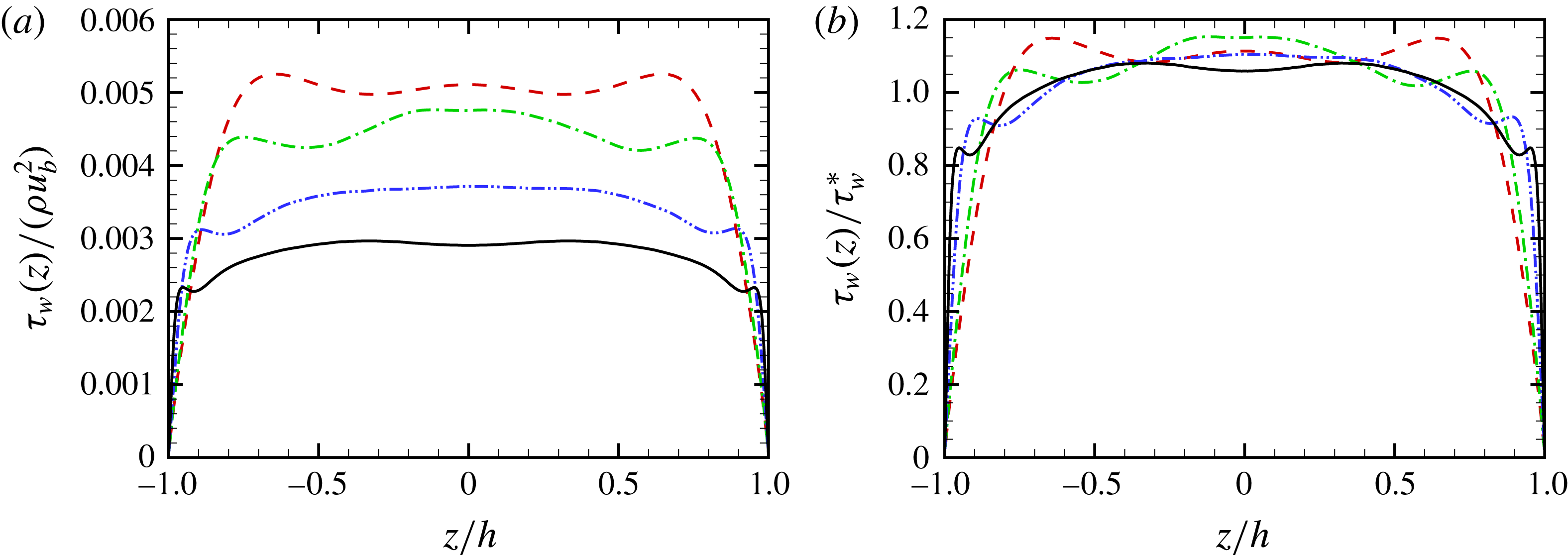
Local wall shear stress along the bottom wall, normalized with respect to the bulk dynamic pressure (a), and with respect to its mean value (b) for flow case A (dashed), B (dash-dot), C (dash-dot-dot), D (solid).

The modulating effect of the secondary motions on the streamwise velocity field is clear in the distributions of the local wall friction (see figure 10). Except for the corner proximity, deviations of the local friction from its mean value are found to be no more than $10\,\%$ . A non-monotonic trend with respect to $Re$ variation is also evident here, with maximum values of the wall friction which are first attained midway between the corner and the wall bisector (flow case A), then at the wall bisector (flow cases B, C), and then again in between at higher Reynolds number. The behaviour observed in flow case D is qualitatively very similar to what was found in experimental measurements (Leutheusser Reference Leutheusser1984), generally carried out at higher Reynolds number, and it is consistent with the previously observed shape of the velocity isolines (see figure 9). Overall, the findings corroborate the theoretical analysis developed by Spalart et al. (Reference Spalart, Garbaruk and Stabnikov2018), which predicts a flat distribution of the wall shear stress as the only possible way of achieving asymptotic matching between the core flow and the near-wall layer.

Figure 11.

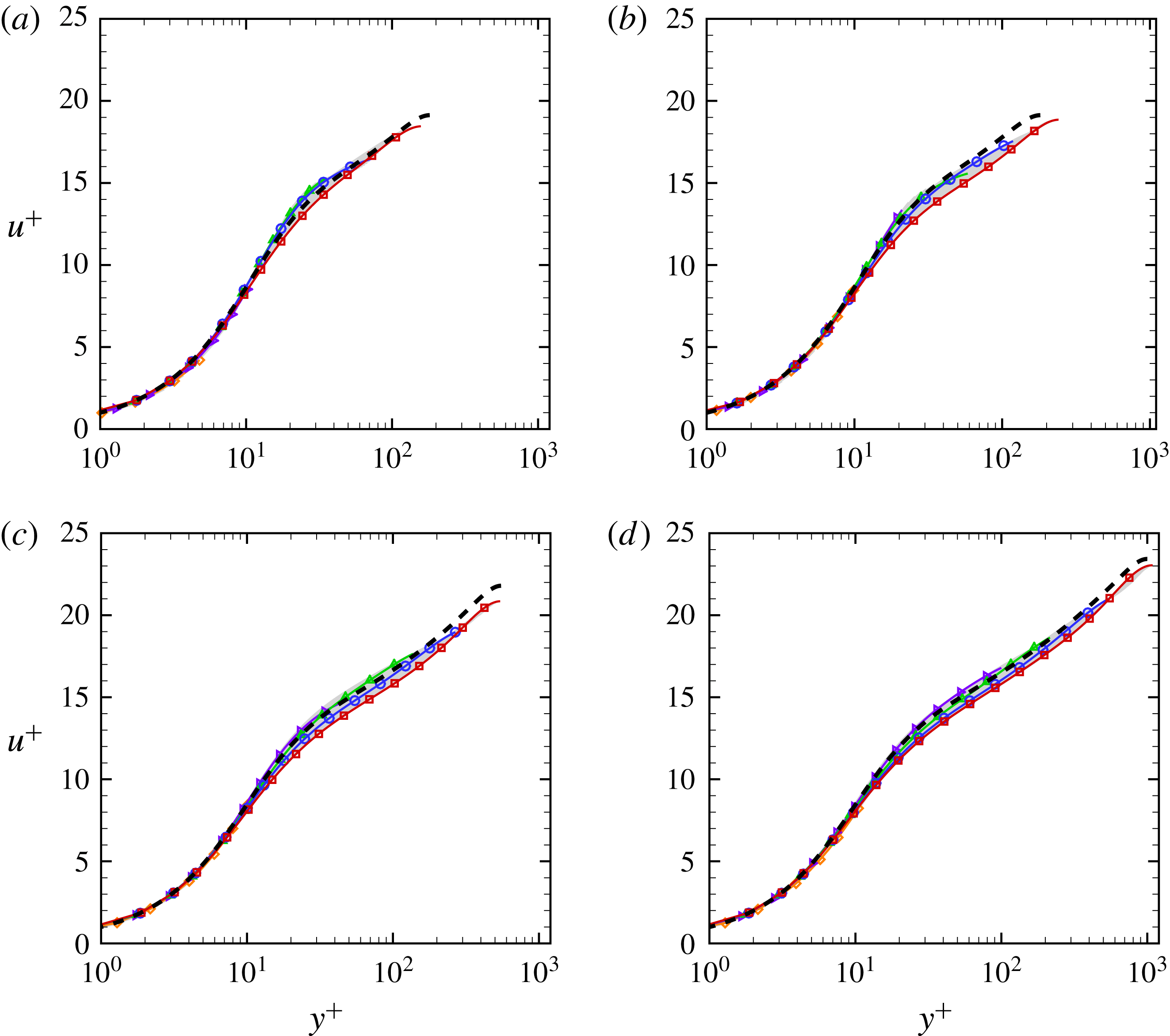
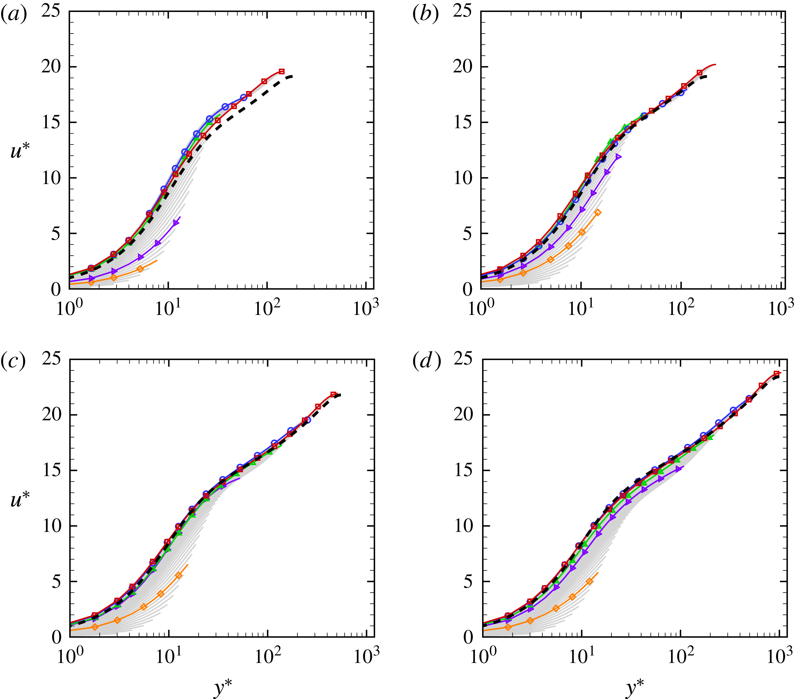
Mean streamwise velocity profiles along the $y$ direction (up to the corner bisector), given in local wall units at all $z$ . Panels (a)–(d) correspond to cases A–D, respectively. Representative stations along the bottom wall are highlighted, namely $z^{\ast }=15$ (diamonds), $(z+h)/h=0.1$ (right triangles), $(z+h)/h=0.25$ (triangles), $(z+h)/h=0.5$ (circles), $(z+h)/h=1$ (squares). The dashed lines denote mean profiles from DNS of pipe flow at $Re_{\unicode[STIX]{x1D70F}}=180$ (a,b), $Re_{\unicode[STIX]{x1D70F}}=550$ (c), $Re_{\unicode[STIX]{x1D70F}}=1000$ (d), from Khoury et al. (Reference Khoury, Schlatter, Noorani, Fischer, Brethouwer and Johansson2013).

Figure 12.

Mean streamwise velocity profiles along the $y$ direction (up to the corner bisector), given in global wall units at all $z$ . Panels (a)–(d) correspond to cases A–D, respectively. Representative stations along the bottom wall are highlighted, namely $z^{\ast }=15$ (diamonds), $z/h=0.1$ (right triangles), $z/h=0.25$ (triangles), $z/h=0.5$ (circles), $z/h=1$ (squares). The dashed lines denote mean profiles from DNS of pipe flow at $Re_{\unicode[STIX]{x1D70F}}=180$ (a,b), $Re_{\unicode[STIX]{x1D70F}}=550$ (c), $Re_{\unicode[STIX]{x1D70F}}=1000$ (d), from Khoury et al. (Reference Khoury, Schlatter, Noorani, Fischer, Brethouwer and Johansson2013).

Figure 13.

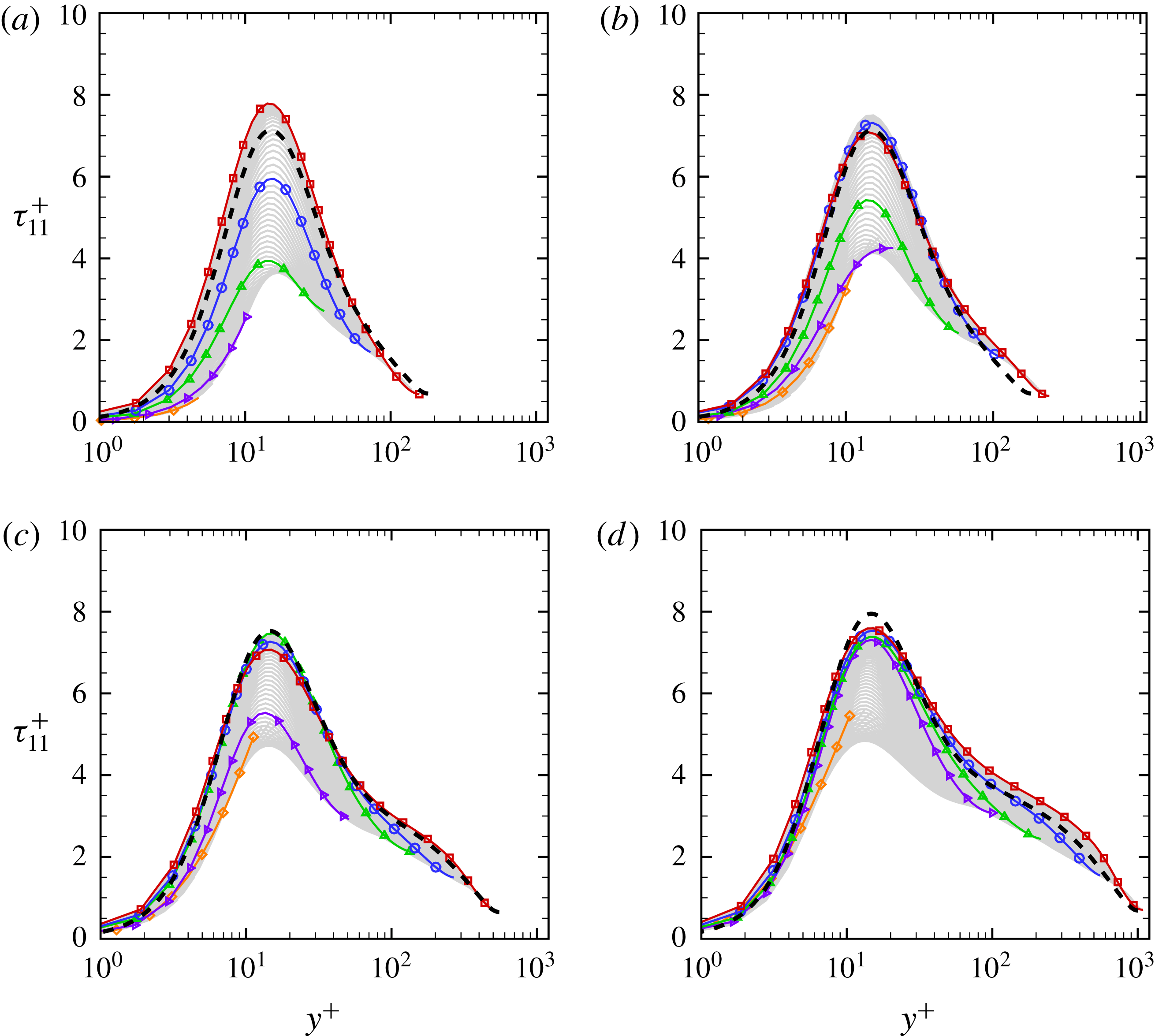
Mean streamwise turbulence intensity profiles along the $y$ direction (up to the corner bisector), given in global local units at all $z$ . Panels (a)–(d) correspond to cases A–D, respectively. Representative stations along the bottom wall are highlighted, namely $z^{\ast }=15$ (diamonds), $z/h=0.1$ (right triangles), $z/h=0.25$ (triangles), $z/h=0.5$ (circles), $z/h=1$ (squares). The dashed lines denote mean profiles from DNS of pipe flow at $Re_{\unicode[STIX]{x1D70F}}=181$ (a,b), $Re_{\unicode[STIX]{x1D70F}}=550$ (c), $Re_{\unicode[STIX]{x1D70F}}=1000$ (d), from Khoury et al. (Reference Khoury, Schlatter, Noorani, Fischer, Brethouwer and Johansson2013).

Based on the previous observations about the near constancy of the wall stress, it is interesting to compare the velocity statistics expressed in local wall units ( $+$ ) and in global wall units ( $\ast$ ). Figure 11 shows the mean velocity profiles as a function of the wall-normal distance up to the corner bisector (where mean velocity attains a maximum), in local wall units. For reference purposes, the mean velocity profiles from DNS of pipe flow at approximately matching $Re_{\unicode[STIX]{x1D70F}}$ are also reported (Khoury et al. Reference Khoury, Schlatter, Noorani, Fischer, Brethouwer and Johansson2013). Excellent collapse of the locally scaled profiles is recovered near the wall, also including the near-corner region. The distributions become more widespread past $y^{+}\approx 10$ , with a maximum scatter of approximately $\pm 5\,\%$ in the ‘logarithmic’ layer. When the mean friction velocity is used for normalization (see figure 12), scatter among the velocity profiles is observed near the wall as a result of the variation of the wall shear stress. Perhaps unexpectedly, this normalization does yield better collapse of the various curves further away from the wall, and near coincidence with the pipe velocity profiles, at least at high enough $Re$ . This finding is probably related to the fact that mean momentum balance (as from (4.1)) is controlled by the imposed spatially uniform pressure gradient rather than by the non-uniform wall shear. Hence it is reasonable that, at least sufficiently away from walls, the flow should respond to the imposed pressure gradient rather than to the wall underneath. Inspection of figure 12 shows that transition from wall scaling to pressure scaling occurs at a wall distance of approximately $0.2h$ , which is also the lower limit for the core region in canonical flows (Pope Reference Pope2000). This interesting effect is impossible to observe in canonical wall-bounded flows, in which the wall shear stress is spatially uniform.

The inner-scaled distributions of the streamwise Reynolds stress are shown in figure 13. Along most of the wall, the behaviour is qualitatively similar to canonical channel flow, with a near-wall peak of $u^{\prime }$ at $y^{+}\approx 12$ . The scatter among the various sections appears to be generally much larger than for the mean velocity field, although it probably becomes confined to the corner vicinity at high $Re$ . An interesting feature is the behaviour of the peak streamwise normal stress with the Reynolds number, which is larger at low $Re$ and then levels off at increasing $Re$ . This apparently contradicts the increasing logarithmic trend of the wall-parallel velocity variances observed in canonical flows (Bernardini, Pirozzoli & Orlandi Reference Bernardini, Pirozzoli and Orlandi2014); hence it would be interesting to carry out DNS at yet higher Reynolds number to verify whether the present observations are related to viscous effects, or whether the mechanisms of inner–outer layer interactions are different in square ducts.

Figure 14.

Terms in the mean streamwise momentum budget (4.1) near the duct corners: mean convection (a,b), turbulence (c,d), viscous diffusion (e,f). (a,c,e) Contour levels for $-0.05\leqslant (\cdot )/({u_{\unicode[STIX]{x1D70F}}^{\ast }}^{2}/\unicode[STIX]{x1D6FF}_{v}^{\ast })\leqslant 0.05$ , in intervals of $0.005$ (dashed lines denote negative values). (b,d,f) Profiles of the budget terms at $y^{\ast }=25$ (dashed lines) and $y^{\ast }=75$ (solid lines) for flow case A (triangles), B (circles), C (diamonds), D (squares).

The terms in the budget of the mean streamwise momentum equation,

are shown in figure 14. Here, the left-hand side represents the contribution of convection from the secondary flows, and the terms on the right-hand side represent the effects of Reynolds stress gradients and viscous diffusion, and the driving pressure gradient. Under global wall scaling (namely, each term is normalized with respect to ${u_{\unicode[STIX]{x1D70F}}^{\ast }}^{2}/\unicode[STIX]{x1D6FF}_{v}^{\ast }$ ), the magnitude of the various terms in the budget is approximately unaffected by $Re$ variation. Away from corners, the leading balance is between the wall-normal turbulent shear stress gradients and viscous diffusion as in canonical flows, whereas mean cross-stream convection is at most one order of magnitude smaller. Convection appears to play a role near corners, where it is responsible for positive momentum transfer, and where it is balanced partly by diffusion and partly by locally negative turbulent stress gradient. This scenario corroborates the previous findings related to the mean velocity profiles (figures 11 and 12). In fact, since convection has a minor effect, logarithmic layers are expected to arise at sufficiently high $Re$ , except in the close vicinity of corners.

Figure 15.

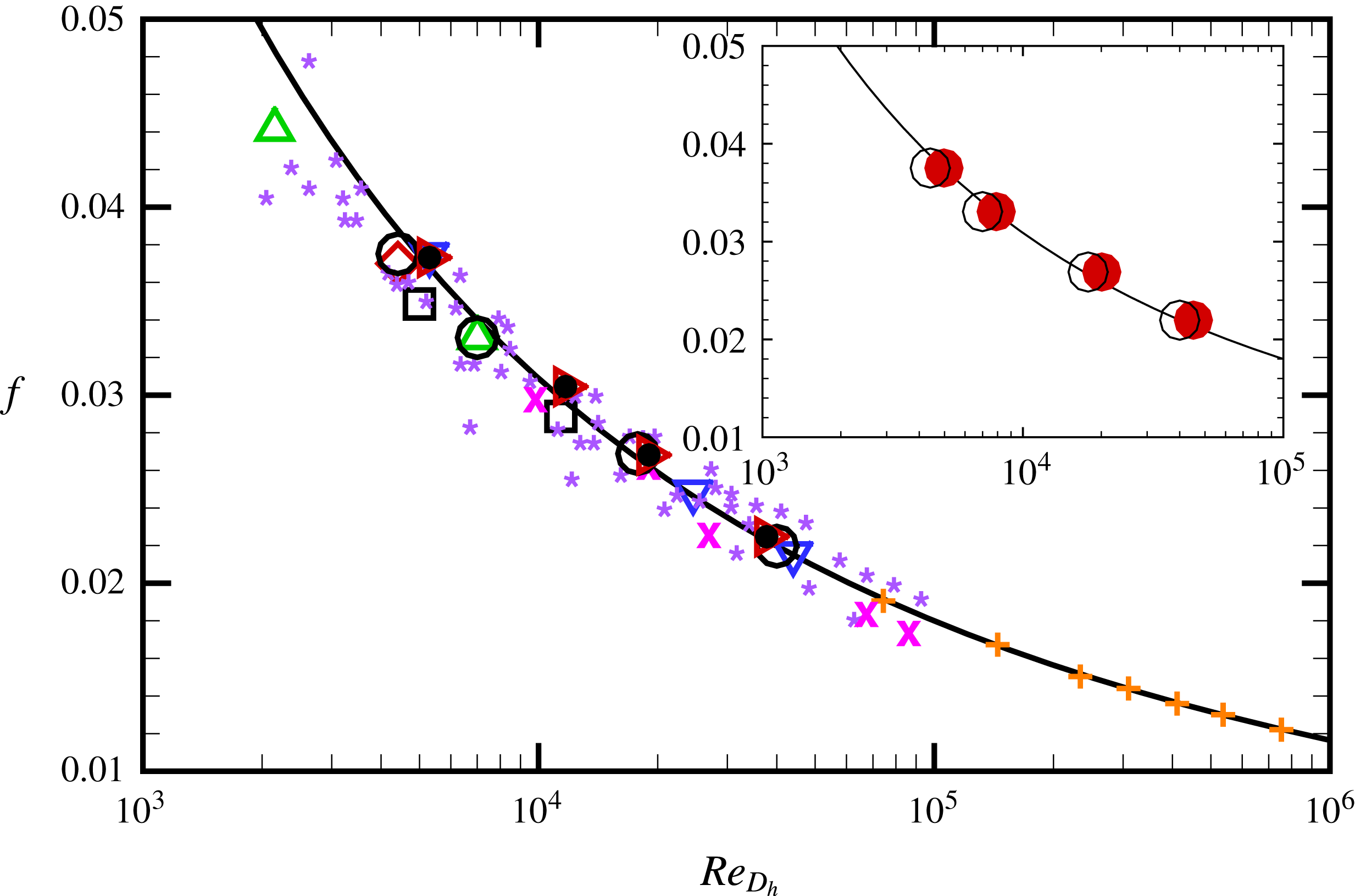
Friction factor ( $f=4C_{f}$ ) as a function of bulk Reynolds number based on the hydraulic diameter ( $Re_{D_{h}}=u_{b}D_{h}/\unicode[STIX]{x1D708}$ ). Solid lines denote the reference friction curve for smooth pipe flow, equation (4.2). Symbols indicate present DNS data (circles), square duct DNS data of Pinelli et al. (Reference Pinelli, Uhlmann, Sekimoto and Kawahara2010) (diamonds) and Vinuesa et al. (Reference Vinuesa, Noorani, Lozano-Durán, Khoury, Schlatter, Fischer and Nagib2014) (squares), square duct experiments by Jones (Reference Jones1976) (stars) and Leutheusser (Reference Leutheusser1963) (crosses), pipe flow DNS data of Wu & Moin (Reference Wu and Moin2008) (down triangles) and Khoury et al. (Reference Khoury, Schlatter, Noorani, Fischer, Brethouwer and Johansson2013) (right triangles), pipe flow experiments by McKeon et al. (Reference McKeon, Li, Jiang, Morrison and Smits2004) (daggers) and hexagonal duct DNS data of Marin et al. (Reference Marin, Vinuesa, Obabko and Schlatter2016) (filled circles). The figure inset shows a comparison with the predictions of the square-root area law (Duan, Yovanovich & Muzychka Reference Duan, Yovanovich and Muzychka2012) (solid circles).

The computed average friction factor, $f=4C_{f}=8\unicode[STIX]{x1D70F}_{w}^{\ast }/(\unicode[STIX]{x1D70C}u_{b}^{2})$ is shown as a function of the bulk Reynolds number in figure 15, together with previous DNS data (Pinelli et al. Reference Pinelli, Uhlmann, Sekimoto and Kawahara2010; Vinuesa et al. Reference Vinuesa, Noorani, Lozano-Durán, Khoury, Schlatter, Fischer and Nagib2014), and assorted experimental data (Jones Reference Jones1976). Overall, the agreement with other DNS is quite good, and results fall well within the scatter of the experimental data points. It is a common notion in the engineering practice (Schlichting Reference Schlichting1979) that friction data for ducts with complex shape should collapse on the friction curves for canonical flows, provided the bulk Reynolds number is constructed using a suitable length scale, the most frequently used being the hydraulic diameter, defined as $D_{h}=4A/P$ , with $A$ the cross-stream area and $P$ the duct perimeter. Hence, $D_{h}=2h$ for a square duct, and $Re_{D_{h}}=Re_{b}$ . Several authors have noticed shortcomings of the hydraulic diameter concept, and proposed alternatives. For instance, Jones (Reference Jones1976) analysed data for rectangular ducts, and came to the conclusion that a corrective factor should be applied to the conventional hydraulic diameter, which happens to be $1.125$ for a square duct. More recently, Duan et al. (Reference Duan, Yovanovich and Muzychka2012) proposed replacing the hydraulic diameter with the square root of the cross-stream area. For the case of a square duct, this correction amounts to multiplying the bulk Reynolds number by a factor $2/\sqrt{\unicode[STIX]{x03C0}}$ , not far from Jones’ correction. For the sake of checking the validity of the above semi-empirical formulations, in figure 15 we also report numerical and experimental data for pipe flow (McKeon et al. Reference McKeon, Li, Jiang, Morrison and Smits2004; Wu & Moin Reference Wu and Moin2008; Khoury et al. Reference Khoury, Schlatter, Noorani, Fischer, Brethouwer and Johansson2013), as well as the Karman–Prandtl theoretical friction law,

Excellent agreement of the DNS data with equation (4.2) is observed using the standard hydraulic diameter formulation, especially for the higher- $Re$ flow cases (C, D). However, proposed corrections to the hydraulic diameter scaling also seem to work very well (see the inset of figure 15), yielding perhaps better agreement at lower Reynolds number.

The success of the hydraulic diameter concept (as well as its variations) may be tentatively explained based on the empirical finding (recalling figure 12 b) that the inner-scaled mean velocity profiles along much of the duct perimeter exhibit near invariance in the outer layer also when scaled with global wall units. Hence, approximating the outer layer profiles with the classical log law, namely $u^{\ast }=1/k\log y^{\ast }+C$ , and integrating over an octant, the following expression for the bulk velocity results:

The friction coefficient can then be evaluated as a function of $Re_{b}$ from (4.3) using $C_{f}=2(u_{\unicode[STIX]{x1D70F}}^{\ast }/u_{b})^{2}$ , $Re_{\unicode[STIX]{x1D70F}}^{\ast }=Re_{b}u_{\unicode[STIX]{x1D70F}}^{\ast }/(2u_{b})$ . Equation (4.3) should be compared with the corresponding expression for a circular duct:

where $Re_{\unicode[STIX]{x1D70F}}=Du_{\unicode[STIX]{x1D70F}}/(2\unicode[STIX]{x1D708})$ , and leading to (4.2). The two expressions become identical provided $2h=D$ ; hence, provided the Reynolds numbers based on the hydraulic diameter are the same. It is interesting that (4.3) is basically arrived at by neglecting the local wall shear stress variation along the duct perimeter, and disregarding the flow deceleration at corners. Apparently, these effects very nearly cancel out when it comes to their contribution to the overall friction.

5 A model for the secondary motions

Based on the outcome of the previous sections a tentative model for the structure of the secondary motions may be formulated. As shown in figure 7, the convective terms in the streamwise vorticity budget are negligible except in the corner proximity. Strict vanishing of the convective terms in (3.2) requires that a functional relationship exists between the average vorticity and streamfunction, namely $\overline{\unicode[STIX]{x1D714}}_{x}=f(\unicode[STIX]{x1D713})$ . 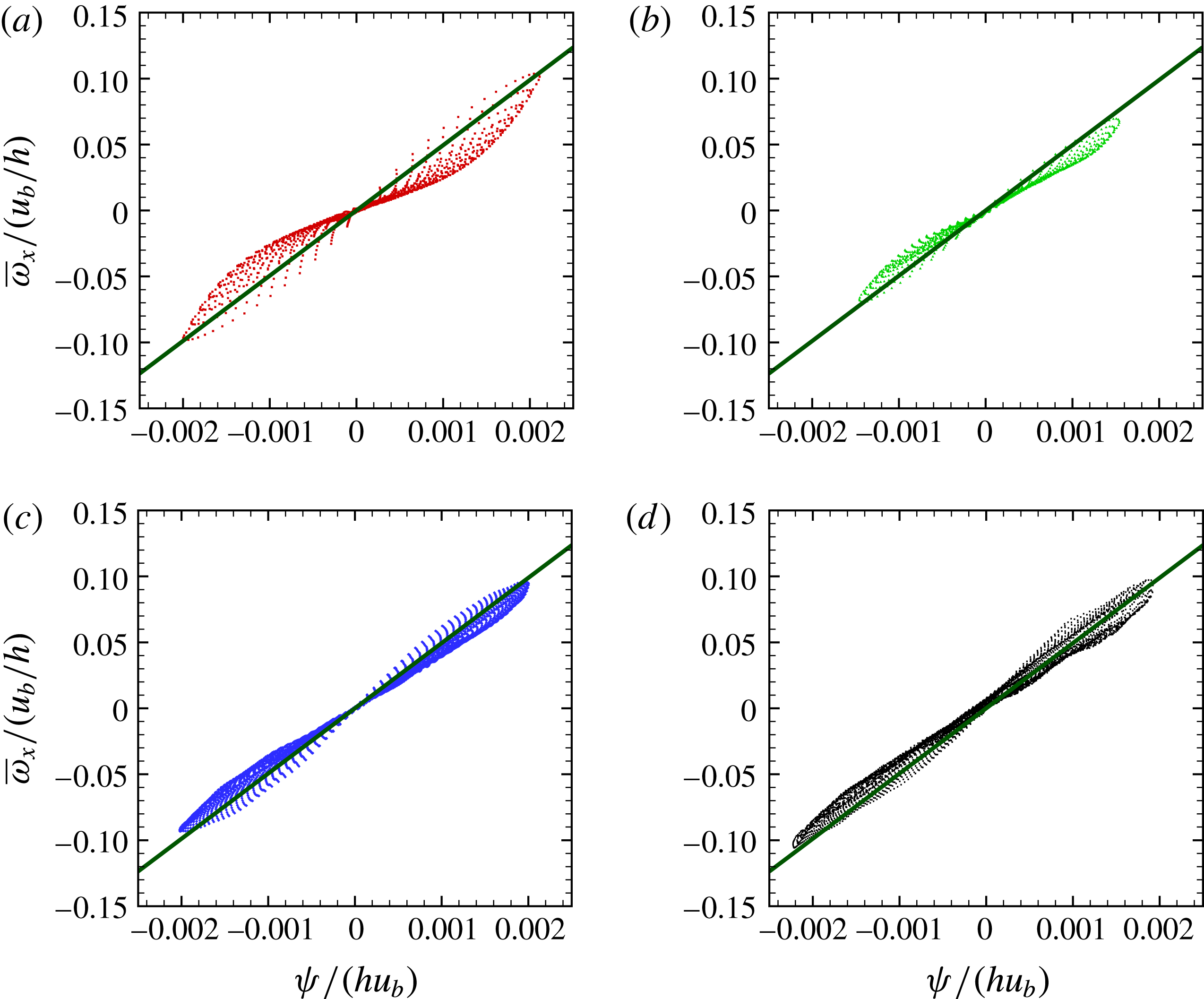This condition is formally equivalent to the necessary condition for the existence of steady solutions in the two-dimensional Euler equations (Batchelor Reference Batchelor1969), although in the present case it applies to the space- and time-averaged statistics of a three-dimensional turbulent flow. This ansatz can be empirically verified based on the DNS data. For that purpose, scatter plots of cross-stream vorticity and streamfunction are shown in figure 16, where points closer to the wall than $0.3h$ have been removed. The data indicate a tendency for $\unicode[STIX]{x1D713}$ and $\overline{\unicode[STIX]{x1D714}}_{x}$ to be more correlated in the duct core as $Re$ is increased. Specifically, a nonlinear relationship is initially identified, which then turns into a distinct linear variation at $Re_{\unicode[STIX]{x1D70F}}^{\ast }\geqslant 500$ . Linear regression of the data shows that $\overline{\unicode[STIX]{x1D714}}_{x}=k^{2}\unicode[STIX]{x1D713}$ , with $k^{2}\approx 49$ . Figure 3 further brings out this increased correlation in physical space, as the isolines of $\overline{\unicode[STIX]{x1D714}}_{x}$ and $k^{2}\unicode[STIX]{x1D713}$ become very similar in the core region as $Re$ is increased.

Figure 16.

Scatter plots of cross-stream vorticity as a function of streamfunction. Panels (a)–(d) correspond to cases A–D, respectively. Only points farther from walls than $0.3h$ are shown. The diagonal line denotes the trend $\overline{\unicode[STIX]{x1D714}}_{x}=k^{2}\unicode[STIX]{x1D713}$ , with $k^{2}=49.373/h^{2}$ .

Assuming a linear dependence between $\overline{\unicode[STIX]{x1D714}}_{x}$ and $\unicode[STIX]{x1D713}$ , it follows from (3.1) that the secondary flow may be approximately characterized in terms of eigenfunctions of the Laplace operator

with $\unicode[STIX]{x1D713}=0$ at the duct boundaries, whereas the no-slip condition clearly cannot be accommodated. The admissible values of $k^{2}$ follow as eigenvalues of (5.1). It is important to note that the steady equation for the streamfunction results from a time-evolving process which is controlled by turbulence production and viscous diffusion. Hence, it may be expected that, in the long term, the only surviving mode(s) will be those which are least damped from viscous diffusion, which occurs for those modes having smaller $k^{2}$ . The first few eigenvalues of (5.1) in a square domain are listed in table 2 – some of them corresponding to multiple eigenfunctions.

Table 2.

List of ten smallest eigenvalues of Laplace operator in a $[-1:1]\times [-1:1]$ square.

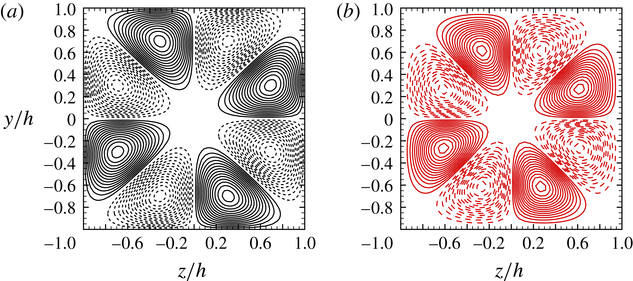
The DNS data (see figure 16) support a value of $k^{2}$ close to the eighth smallest eigenvalue ( $k^{2}=49.373/h^{2}$ ). Notably, the corresponding eigenmode (see figure 17 a) is the first to exhibit the same eight-fold geometrical symmetry as the secondary motions from DNS, and hence with streamlines bisecting the duct corners and satisfying the physical requirement that momentum is transferred from the bulk flow into the corner region.

Figure 17.

Eigenfunctions of (5.1) with $k^{2}=49.373/h^{2}$ (a), and of (5.2) with $\unicode[STIX]{x1D706}^{2}=67.280/h^{2}$ (b).

A mathematical model for the secondary eddies in low-Reynolds-number flow was previously also proposed by Wedin et al. (Reference Wedin, Biau, Bottaro and Nagata2008) based on the concept of a self-sustained process (SSP), and yielding secondary motions as eigensolutions of

with homogeneous boundary conditions for $\unicode[STIX]{x1D713}$ and its wall-normal derivative. Eight eddies geometrically similar to those observed in developed flow are recovered for one particular eigenmode of (5.2) (corresponding to $\unicode[STIX]{x1D706}^{2}=67.280/h^{2}$ ) whose shape is shown in figure 17(b), which is not qualitatively different from the Laplace eigenfunction of (a). However, its $\unicode[STIX]{x1D713}$ – $\overline{\unicode[STIX]{x1D714}}_{x}$ signature (not shown) features clustering of the data points around $\unicode[STIX]{x1D714}_{x}=\unicode[STIX]{x1D706}^{2}\unicode[STIX]{x1D713}$ , and hence quite different from that found in DNS (recalling figure 16).

Figure 18.

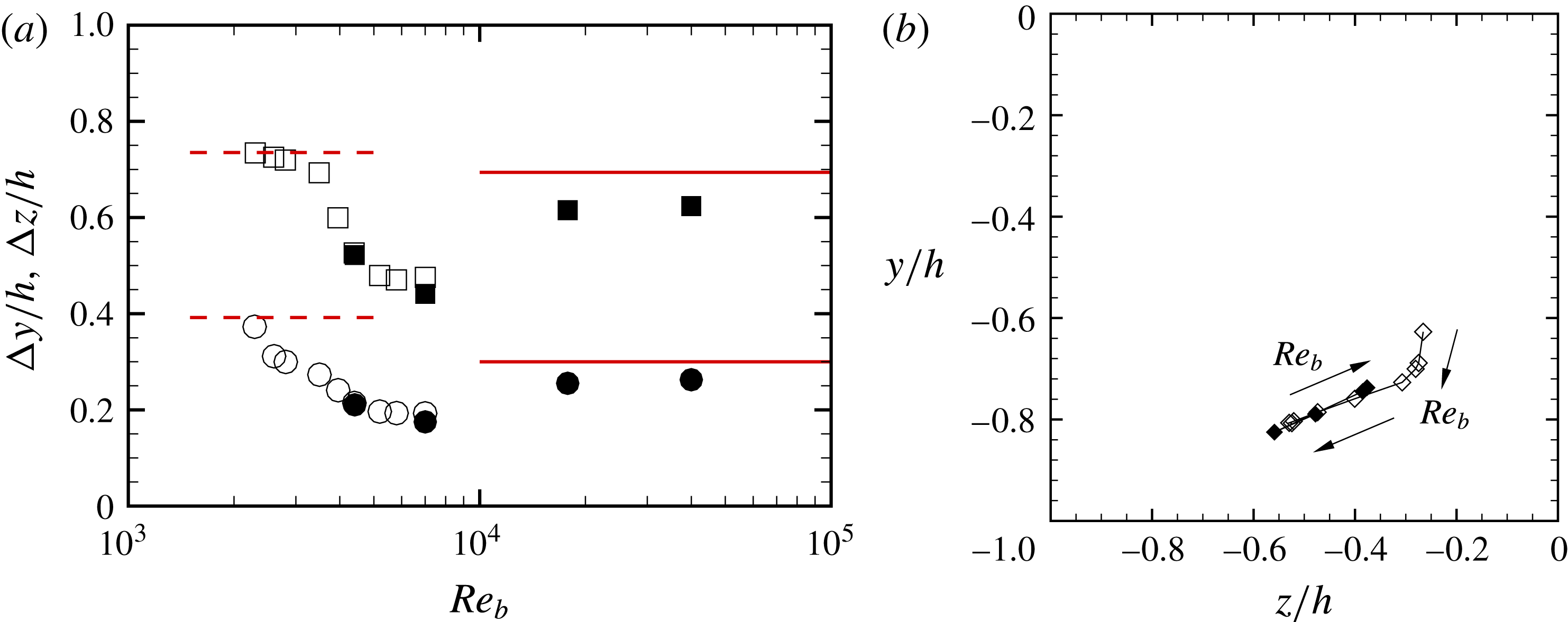
Position of vortex centres: (a) distance from bottom wall as a function of Reynolds number (circles) and from left wall (squares); (b) location in the cross-stream plane. Solid symbols denote the present DNS data, open symbols denote DNS data of Pinelli et al. (Reference Pinelli, Uhlmann, Sekimoto and Kawahara2010). In (a) solid lines denote the vortex centres for eigensolutions of (5.1) with $k^{2}=49.373/h^{2}$ , and dashed lines for eigensolutions of (5.2) with $\unicode[STIX]{x1D706}^{2}=67.280/h^{2}$ .

More quantitative evaluation of the properties of the secondary eddies can be gained from figure 18, where we show the distance of the cross-stream vortex centres from the duct walls as a function of the Reynolds number. Low-Reynolds-number data from Pinelli et al. (Reference Pinelli, Uhlmann, Sekimoto and Kawahara2010) are also shown. A non-monotonic drift of the vortex centre position is found at low Reynolds number, whereby centres initially approach the corner, and then move away from it. Interestingly, it appears that the predictions of the SSP theory (Wedin et al. Reference Wedin, Biau, Bottaro and Nagata2008) are in good agreement with DNS at low $Re$ , whereas the Laplace eigenfunctions reproduce the asymptotic trend at high Reynolds number.