1. Introduction
The adverse effects of climate change are experienced worldwide (Dell et al., Reference Dell, Jones and Olken2012, Reference Dell, Jones and Olken2014; Graff Zivin and Neidell, Reference Graff Zivin and Neidell2014; Burke et al., Reference Burke, Hsiang and Miguel2015; Colacito et al., Reference Colacito, Hoffmann and Phan2019; Acevedo et al., Reference Acevedo, Mrkaic, Novta, Pugacheva and Topalova2020; Dang et al., Reference Dang, Hallegate and Trinh2024), and poor countries are even more affected (Kahn, Reference Kahn2005; Shepherd et al., Reference Shepherd, Mitchell, Lewis, Lenhardt, Jones, Scott and Muir-Wood2013; IPCC, 2014; Tol, Reference Tol2018; Winsemius et al., Reference Winsemius, Jongman, Veldkamp, Hallegatte, Bangalore and Ward2018; Hallegate et al., Reference Hallegate, Vogt-Schilb, Rozenberg, Bangalore and Beaudet2020; Chancel et al., Reference Chancel, Bothe and Voituriez2023). In developing countries, climate change impacts women more than men (Denton, Reference Denton2002; Goh, Reference Goh2012; Björnberg and Hansson, Reference Björnberg and Hansson2013; Sorensen et al., Reference Sorensen, Murray, Lemery and Balbus2018; Quisumbing et al., Reference Quisumbing, Kumar and Behrman2018) and creates challenges for gender equity and economic growth. Women have lower resilience capacities to cope with the impacts of climate change because of unequal access to productive resources such as land or other assets (Deressa and Hassan, Reference Deressa and Hassan2009; Terry, Reference Terry2009; Mehar et al., Reference Mehar, Mittal and Prasad2016; Mersha and Van Laerhoven, Reference Mersha and Van Laerhoven2016; Eastin, Reference Eastin2018). Many women work in climate-sensitive sectors such as agriculture or tourism and face significant gender gaps in salary (SOFA Team and Doss, Reference Doss2011; Doss et al., Reference Doss, Kovarik, Peterman, Quisumbing and van den Bold2015, Reference Doss, Meinzen-Dick, Quisumbing and Theis2018; Doss Reference Doss2018). Women are mainly responsible for domestic work, which reduces their time available for economic opportunities (Elson, Reference Elson1999; Fontana and Van Der Meulen Rodgers, Reference Fontana and Van Der Meulen Rodgers2005). The impacts of climate change increase the time requirements for domestic work and widen the gaps between paid and unpaid work. Indeed, after floods, it takes longer for women to fetch water or collect wood, reducing the available time for paid activity. Understanding the nexus between climate change and gender, with its sectoral and socio-economic impacts, is the basis for designing counteracting policies to mitigate the impacts of climate change on women (Denton, Reference Denton2002; Terry, Reference Terry2009; Alston, Reference Alston2014; Pearse, Reference Pearse2017).
While women’s vulnerability to climate change poses challenges both for their own well-being and for their economic participation, the negative impacts also extend to population groups that are even more vulnerable, namely, the children and elderly for whom women are typically responsible. Thus, the impacts of climate change are not only experienced directly by women but are also transmitted through them to these more vulnerable groups.
In South Africa, women play a key role in economic growth and face high gender inequalities (Department of Women, 2015). The country is exposed to the impacts of climate change (Ziervogel et al., Reference Ziervogel, New, Archer van Garderen, Midgley, Taylor, Hamann, Stuart-Hill, Myers and Warburton2014; DEA (Department of Environmental Affairs), 2016; Ayugi et al., Reference Ayugi, Eresanya, Onyango, Ogou, Okoro, Okoye, Anoruo, Dike, Ashiru, Daramola, Mumo and Ongoma2022), which may increase gender inequalities to the disadvantage of women (Flatø et al., Reference Flatø, Muttarak and Pelser2017). The labour participation rate is lower for women than for men; in 2023, it was 54.3 per cent for women and 64.9 per cent for men (Stats SA, 2023). Women work mainly as low-skilled workers (Espi et al., Reference Espi, Francis and Valodia2019; Gradín, Reference Gradín2021) and in a narrow range of sectors: agriculture, food processing, textiles and tourism (Mosomi, Reference Mosomi2019). The unemployment rate is higher for women than for men (e.g., in 2024, it was 31.6 per cent for women and 27.6 per cent for men (ILO, 2024)). Furthermore, women work significantly more time carrying out domestic tasks than men. While women work on average 4.36 hours per day – unpaid for domestic tasks – men work only 2.16 hours per day for unpaid domestic tasks (Budlender et al., Reference Budlender, Chobokoane and Mpetsheni2001; Charmes, Reference Charmes and Blackden2006). With lower access to the paid labour market and lower-paid salaries, women experience higher rates of poverty (Sulla and Zikhali, Reference Sulla and Zikhali2018), which is likely to worsen with the future impacts of climate change. Shayegh et al. (Reference Shayegh, Manoussi and Dasgupta2021) find that in South Africa, high temperatures reduce the weekly labour supply more sharply for ‘low-skilled’ than for ‘high-skilled’ South African workers. Moreover, Shayegh and Dasgupta (Reference Shayegh and Dasgupta2022) find that the working hours of South African low-skilled women are more impacted by the effects of higher temperatures.
Various studies have analysed the impacts of climate change on women (see Chitiga-Mabugu et al., Reference Chitiga-Mabugu, Henseler, Maisonnave and Mabugu2023, for a review). Earlier studies described the general impacts qualitatively (e.g., Denton, Reference Denton2002; Pearse, Reference Pearse2017). Later studies focused on specific impacts and provided quantitative analysis, e.g., of impacts on women in the agricultural sector (Eastin, Reference Eastin2018). Finally, recent studies have extended the scope from gendered impacts to women’s role in climate change adaptation and mitigation (e.g., Huyer and Partey, Reference Huyer and Partey2020; Gardezi et al., Reference Gardezi, Michael, Stock, Vij, Ogunyiola and Ishtiaque2022). However, while these studies provide valuable information on sector-specific impacts and measures at the microeconomic level, they do not provide information about economy-wide impacts at the macroeconomic level.
In the present article, we analyse the sector-specific impacts of climate change on women in South Africa and the microeconomic impacts on poverty among women. To simulate and analyse the macroeconomic impacts, we use a recursive dynamic computable general equilibrium (CGE) model; to analyse the microeconomic impacts, we apply a distributional analysis as a microsimulation and poverty analysis.
CGE models have been used to analyse the climate impact in South Africa. For instance, Calzadilla et al. (Reference Calzadilla, Zhu, Rehdanz, Tol and Ringler2014) employ a CGE model to find the significant impacts of climate change on agricultural production and economic growth. Decreasing precipitation reduces the national GDP by 0.6 per cent. Compensating for these losses requires an increase in productivity of 20 per cent. Using a CGE model, Cullis et al. (Reference Cullis, Alton, Arndt, Cartwright, Chang, Gabriel, Gebretsadik, Hartley, de Jager, Makrelov, Robertson, Schlosser, Strzepek and Thurlow2015) simulate the impacts of different economic shocks on agriculture, water supply and infrastructure. They find a decrease in South Africa’s GDP by up to 3.8 per cent. Climate change mainly impacts agriculture, which reduces production, while non-agricultural sectors expand. Consequently, many unskilled workers change from agricultural to non-agricultural sectors. Poverty is exacerbated, particularly in the poor regions of the country.
Recent studies have employed a gender-sensitive CGE model to analyse the impact of climate change on women in Western Africa and Latin America. Sawadogo and Fofana (Reference Sawadogo and Fofana2021) show that in Burkina Faso, climate change impacts women’s economic activities more than men’s economic activities. For Bolivia, Escalante and Maisonnave (Reference Escalante and Maisonnave2022a) find that female-headed households (FHHs) in particular suffer from the impacts of climate change due to a decrease in income and increased food prices. Furthermore, they find that mainly female labour is affected, as women drop out of the labour market, and that FHHs experience more increases in poverty than male-headed households (MHHs). In another paper, Escalante and Maisonnave (Reference Escalante and Maisonnave2022b) show that in Bolivia, women’s food security is particularly vulnerable, depending on the regional climate impacts on agricultural production.
This paper builds on previous studies and aims to make several contributions. First, we build a recursive dynamic gender-aware CGE model that considers domestic production, where unpaid household chores are mainly carried out by women. Second, we consider the impacts on different sectors of the economy, not only agricultural sectors. Indeed, we consider the potential drop in the tourism sector as well as problems in the water sector. Third, we assess the socio-economic impact of climate disasters on women’s poverty. Thus, this study draws attention to a phenomenon that is still largely unquantified in the literature and that will make it possible to implement specific policies for women.
2. Method
We use a recursive dynamic CGE model combined with a microsimulation to evaluate the impacts of climate change on women’s poverty in South Africa. CGE models are appropriate tools for simulating and analysing the direct and indirect impacts of climate change on the different institutions in an economy. We then link the CGE model with the microsimulation model to assess the redistributive impacts of climate change on poverty.
2.1. Macroeconomic model
To represent the South African economy, we develop a recursive dynamic single-country CGE model by customizing the CGE standard model PEP-1-t (Decaluwé et al., Reference Decaluwé, Lemelin, Robichaud and Maisonnave2013). Figure 1 presents schematically the CGE model with its markets, institutions, agents and sectors with their monetary flows and interlinkages.Footnote 1
Schematic presentation of a CGE model.

Figure 1 Long description
The schematic presents a CGE model with various components and their interactions. The government is linked to investment savings through fiscal surplus and investment in the next period. The factor market connects to households via factor income and to the commodity market through intermediate consumption. Households engage in private consumption and receive transfers. The commodity market interacts with production sectors like agriculture, mining and services and is involved in imports and exports with the rest of the world. Arrows indicate the flow of monetary values and interlinkages between these entities.
The database used for the CGE model is a 2015 Social Accounting Matrix (SAM) based on that of van Seventer and Davis (Reference van Seventer and Davis2019). We disaggregate the 2015 SAM by gender-specific concerning labour types and households using the National Income Dynamics Study 2015 and the Living Conditions Survey 2015. Consequently, the sectors are aggregated into the 10 sectors identified in the National Income Dynamics Study.
We include 10 activities and 19 commodities in the model, with each activity using capital, labour (skilled and unskilled) and intermediate goods consumption to produce output. Production follows a Leontief-type function between value-added and intermediate consumption at the top level and for each activity. Value-added is a constant elasticity of substitution (CES) function of composite labour and capital. Composite labour is disaggregated based on skill levels following a CES function (skilled and unskilled). Skilled workers have at least completed secondary education (grade 12), while unskilled workers have a middle school education at most (maximum grade 11). At the bottom of the tree, each type of labour is disaggregated into male and female, representing workers as men and women. We assume imperfect substitutability between male and female workers, represented by a CES function. The elasticity of substitution is set lower among skilled workers than among unskilled workers, reflecting more specialized and less interchangeable roles.
Each activity uses intermediate inputs, capital and the different types of labour, although in different proportions. For instance, a sector such as manufacturing relies mainly on intermediate consumption to produce (75.6 per cent of its production) while another sector, such as public administration, intensively uses labour, and among labour, mainly skilled female workers. The water sector, which is one of the climate-sensitive sectors, is capital-intensive, and its workforce is mainly composed of skilled male workers. In South Africa, certain sectors remain highly male-intensive, particularly mining, construction and transport, where men account for more than 80 per cent of the workforce. The agricultural sector is somewhat less male-intensive, yet men still constitute around 70 per cent of its labour force. By contrast, sectors such as tourism and catering, public administration and financial services employ a relatively high share of skilled women. Recognizing these gendered patterns of employment is important for interpreting the results of the simulations that follow.
In the model, we distinguish four different institutions: households, firms, the government and the rest of the world. Households are disaggregated per decile of income and gender and receive income from labour, capital and transfers. Poor households with small incomes mainly receive transfers from the government and income from unskilled labour. For example, 73.7 per cent of the income of households in the first decile comes from government transfers and a little less than 25 per cent comes from unskilled work income (male and female). The richest households mainly receive income from dividends and highly skilled labour. Households use their income to pay taxes or transfers to other institutions, to consume and to save. Households in the lowest five deciles spend more than 95 per cent of their income on consumer spending. This share falls to 55 per cent for households in the highest decile. Household consumption is modelled as a linear expenditure system subject to budget constraints. Firms derive their income from capital and transfers from other institutions. They pay income taxes and transfers to other institutions (dividends). The government's income is derived from direct taxes paid by households and firms (35.3 per cent of its income), indirect taxes on domestic sales (22.2 per cent), import tariffs, activity tax, transfers from other institutions, and a share of capital income. Government savings equal the government’s income minus its consumption and transfers paid to other institutions.
Capital is sector specific, and the stock of capital of each sector depends on the new investments made in the sector in the previous period. The allocation of new investment follows the accumulation equation (Jung and Thorbecke, Reference Jung and Thorbecke2003). Labour is mobile across sectors. Following the work of Fofana et al. (Reference Fofana, Cockburn and Decaluwé2003), we consider an endogenous gendered labour supply subject to the time that households devote to their market and nonmarket activities. We consider that each individual in the household has a fixed number of hours to allocate between leisure, paid work and unpaid work for the production of nonmarket commodities, e.g., childcare, cooking and firewood and water collection.
As mentioned earlier, South African women with primary education spend, on average, 4.48 hours per day on unpaid activities and 2.20 hours per day on paid activities. Men spend 2.36 hours per day on unpaid activities and 6.18 hours per day on market activities. The time spent on domestic tasks decreases with the increase in the level of education for both men and women. Skilled women (with tertiary education) spend 3.59 hours per day on unpaid activities and 4.70 hours per day on paid activities; skilled men spend 1.91 hours per day on unpaid activities and 6.03 hours per day on paid activities (Rubiano-Matulevich and Viollaz, Reference Rubiano-Matulevich and Viollaz2019).
Technically, following Fofana et al. (Reference Fofana, Cockburn and Decaluwé2003), we assume that households maximize their utility by allocating their time between paid and unpaid work and leisure under the constraint of their full income. Full income is the sum of the different incomes from paid work, non-labour incomes (such as transfers) and income from home production, which is valued as its opportunity cost on the labour market. The production function for home production is a CES function between male and female labour, disaggregated by skills. The allocation of labour between women and men is influenced by the extent to which they are substitutable and by their respective opportunity costs, proxied by the average wages prevailing in the labour market. By defining a low value of substitution elasticity, we reflect the rigidity between male and female labour (Fontana and Wood, Reference Fontana and Wood2000; Fontana et al., Reference Fontana, Byambasuren and Estrades2020; Koinda et al., Reference Koinda, Montaud, Souratié and Dite2025). Under this framework, the labour supply, measured in hours, is endogenously derived from households’ time-allocation choices. In the labour market, it equilibrates with the demand for labour from economic activities through wage flexibility, resulting in a full-employment equilibrium.
Additional data, such as income elasticity from Burger et al. (Reference Burger, Coetzee, Kreuser and Rankin2017) and trade elasticities from Ntombela et al. (Reference Ntombela, Kalaba and Bohlmann2018), are used to operationalize the model further. We model the trade between South Africa and the rest of the world based on the assumption of the imperfect substitutability of commodities given their origin (the Armington assumption). We assume a finite elasticity of export demand to reflect the competitiveness of local producers in international markets. South African producers need to be more competitive than foreign producers to increase their global market shares. In terms of closure rules, the nominal exchange rate is the numeraire. The rest of the world’s savings are assumed to be fixed. Finally, South Africa takes world prices as given, which follows from the assumption that the country is a small open economy.
2.2. Microeconomic model
CGE models alone cannot provide insights into the impacts of climate change on poverty. To enable such explicit poverty and distributional analysis, we link the CGE model to a micro module using a top-down approach, as presented by Cockburn et al. (Reference Cockburn, Savard, Tiberti and O'Donoghue2014). In each scenario, we apply the percentage changes in households’ consumption spending to the households in the microdata, i.e., the Living Condition Survey 2014–2015 (Stats SA, 2017a). Furthermore, we apply the percentage change in the consumer price to the poverty line and simulate the change in purchasing power. For each scenario, we compute the poverty index based on Foster et al. (Reference Foster, Greer and Thorbecke1984) and compare the change in indicators to the business-as-usual (BAU) scenario. We compute the indicators for the national sample and regional sample oriented towards Stats SA (2018, 2019).
3. Scenarios
To analyse the impacts of climate change on the economy and women, we simulate two scenarios: a ‘moderate scenario’ and a ‘severe scenario’. We orient them towards the policy scenarios presented by Fawcett et al. (Reference Fawcett, Iyer, Clarke, Edmonds, Hultman, McJeon, Rogelj, Schuler, Alsalam, Asrar, Creason, Jeong, McFarland, Mundra and Shi2015): the ‘reference-low policy scenario’ and the ‘no-policy scenario’. The ‘reference-low policy scenario’ is the basis for our ‘moderate scenario’, which assumes a moderate increase in global greenhouse gas emissions until 2100 and mild-to-moderate economic impacts. The ‘no-policy scenario’ is the basis for our ‘severe scenario’, which assumes an extreme increase in greenhouse gas emissions until 2100 and strong economic impacts. We assume that climate shocks will impact the economy through different channels in the agricultural and non-agricultural sectors. Therefore, we highlight five channels through which weather shocks can affect the economic sectors in South Africa:
(1) Climate change decreases agricultural productivity through changes in precipitation, temperature, climate variability, evapotranspiration and freshwater availability (Calzadilla et al., Reference Calzadilla, Zhu, Rehdanz, Tol and Ringler2014; Aragon et al., Reference Aragon, Oteiza and Rud2021). In addition to the direct impact on crop productivity, climate change can increase yield losses caused by pests (e.g., locust infestation) and soil degradation. Furthermore, harvest and production factors can be lost due to extreme weather events (floods, droughts). We derive the shocks of climate impacts on agricultural productivity from the studies by Tadesse (Reference Tadesse2010), Calzadilla et al. (Reference Calzadilla, Zhu, Rehdanz, Tol and Ringler2014) and Cullis et al. (Reference Cullis, Alton, Arndt, Cartwright, Chang, Gabriel, Gebretsadik, Hartley, de Jager, Makrelov, Robertson, Schlosser, Strzepek and Thurlow2015).
(2) Climate change negatively impacts agricultural production in most countries worldwide. Thus, the supply of agricultural commodities for export markets decreases, while the demand in import markets increases. Additionally, climate change increases competition for land (e.g., between food and energy production or mining), and increasing demand caused by an increasing population increases the demand for food and food prices (Wheeler and Von Braun, Reference Wheeler and Von Braun2013). We derive the magnitude of changes from Baker et al. (Reference Baker, Havlík, Beach, Leclère, Schmid, Valin, Cole, Creason, Ohrel and McFarland2018), Dumortier et al. (Reference Dumortier, Carriquiry and Elobeid2021) and the World Bank (2022b), and we apply the same dynamic to the shocks to productivity.
(3) While changes in water demand for agricultural supply (e.g., irrigation) and precipitation are represented as impacts on agricultural productivity, the decrease in water supply for households and industry is assumed to decrease. The decrease in piped water supply for households and industry comes from an increase in capital costs for water producers, which translates into an increase in water prices. Extreme weather events, droughts, irregular precipitation and continuously increasing evapotranspiration reduce the availability of water in water bodies, decreasing the supply of water. We derive the magnitude of shocks from the studies by Cullis et al. (Reference Cullis, Alton, Arndt, Cartwright, Chang, Gabriel, Gebretsadik, Hartley, de Jager, Makrelov, Robertson, Schlosser, Strzepek and Thurlow2015), Olabanji et al. (Reference Olabanji, Ndarana, Davis and Archer2020) and Du Plessis and Kalima (Reference Du Plessis and Kalima2021).
(4) Weather events impact tourism (Thomas et al., Reference Thomas, Wilhelmi, Finnessey and Deheza2013), e.g., extreme weather events, and the reduction of sightseeing goals (such as ecosystems for safaris) reduces attractiveness. Weather events affect transport, infrastructure and tourism activities. The extremes in temperature and changes in weather patterns can impact the attractiveness of tourist destinations (Golder Associates, 2011). Based on the study by Mathivha et al. (Reference Mathivha, Tshipala and Nkuna2017) on international tourism arrivals and research on annual temperature and precipitation by the World Bank (2022a, 2022c), we compute the decrease in tourism arrivals for historical years, which we use to derive the scenario assumptions. Many women work in the tourism service sector (hotels, restaurants). Thus, fewer tourists negatively impact women’s jobs in this sector. By also demanding food for restaurants, the impacts on the tourism sector spill over to the agri-food sector. Gray et al. (Reference Gray, Taraz and Halliday2023) show that drought negatively impacts the tertiary sector and, specifically, the tourism sector in South Africa.
(5) Capital depreciation: As noted by Fankhauser and Tol (Reference Fankhauser and Tol2005) and Stern (Reference Stern2013), it is likely that climate change will impact the depreciation rate of capital, consequently affecting the longevity of the capital stock. Extreme weather events such as floods can cause permanent damage to capital infrastructure. Being exposed to an extreme event can increase wear and tear and, consequently, a larger amount of investment will be used to compensate for the depreciation (Dietz and Stern, Reference Dietz and Stern2015; Tsigaris and Wood, Reference Tsigaris and Wood2019). To take this phenomenon into account in our model, we increase the rate of depreciation for affected sectors (agriculture and tourism) starting in 2030. The increase is constant over time and the same for both scenarios. Specifically, we increase the depreciation rate by two percentage points, setting it at 6 per cent from 2030 onward and only for the agriculture and water scenario.
We simulate the period from 2015 to 2050. To represent the short- and medium-term impacts, we apply shocks with increasing magnitude from 2025 to 2040. To simulate the long term, we retain the magnitude of 2040 for the years after 2040. Finally, we compare the scenarios with the BAU scenario, which follows a steady path from 2015 to 2050 without climate change shocks. Table 1 presents the assumptions for the simulated shocks, while Figure 2 presents schematically the CGE model with the simulated economic shock on agricultural productivity and markets, water supply and tourism demand.
Schematic presentation of the channels impacted in the CGE model.

Figure 2 Long description
The diagram illustrates an economic model with various components and impacts. Arrows indicate the flow of monetary value and resources between these components. The model highlights shocks on agricultural productivity, water supply, agricultural prices and tourism demand. The government interacts with the rest of the world through taxes and transfers. Households receive income and make private consumption. The factor market deals with factor income and savings, while the commodity market handles the supply and demand of goods and services. The diagram uses different colors to represent the various shocks impacting the model.
Overview of the assumptions of the simulated scenario impacts (in per cent deviation from the baseline, except for capital depreciation)

Table 1 Long description
The table compares the impacts of moderate and severe scenarios on agricultural productivity, capital depreciation, agricultural trade, freshwater supply, and tourism demand from 2025 to 2040. In severe scenarios, agricultural productivity declines by 25% by 2040, while world prices increase by 40%. Both scenarios show consistent capital depreciation at 0.06% by 2040. Freshwater supply productivity decreases by 25% in severe scenarios, and tourism demand drops by 13%. The data suggests more significant impacts in severe scenarios, with linear interpolation used for 2030 values.
a In the years between 2025 and 2040, the shock gradually increases. The table is represented as linear interpolation in 2030.
b Based on the results and assumptions of Calzadilla et al. (Reference Calzadilla, Zhu, Rehdanz, Tol and Ringler2014), Cullis et al. (Reference Cullis, Alton, Arndt, Cartwright, Chang, Gabriel, Gebretsadik, Hartley, de Jager, Makrelov, Robertson, Schlosser, Strzepek and Thurlow2015) and Tadesse (Reference Tadesse2010).
c We derive the magnitude of changes from Baker et al. (Reference Baker, Havlík, Beach, Leclère, Schmid, Valin, Cole, Creason, Ohrel and McFarland2018), Dumortier et al. (Reference Dumortier, Carriquiry and Elobeid2021) and the World Bank (2022a).
d We derive the magnitude of changes from Cullis et al. (Reference Cullis, Alton, Arndt, Cartwright, Chang, Gabriel, Gebretsadik, Hartley, de Jager, Makrelov, Robertson, Schlosser, Strzepek and Thurlow2015), Olabanji et al. (Reference Olabanji, Ndarana, Davis and Archer2020) and Du Plessis and Kalima (Reference Du Plessis and Kalima2021).
e We derive the magnitude of changes from Mathivha et al. (Reference Mathivha, Tshipala and Nkuna2017).
4. Results and discussion
4.1. Macroeconomic impacts
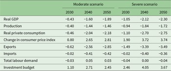
Table 2 presents the changes in macroeconomic indicators and provides information about the scenario impacts on the whole economy. The simulated impacts of climate change result in decreased aggregated economic performance, represented by a decrease in real GDP. In the moderate scenario, in 2050, real GDP decreases by 1.89 per cent, and in the severe scenario, it decreases by 2.30 per cent (Table 2). The negative impacts on production and the increase in world market prices for agricultural commodities create an increase in production costs and commodity prices (Appendix Tables A1(c) and (d)). The increase in costs and commodity prices is reflected by the increasing consumer price index and a decrease in private consumption (−2.18 and −2.75 per cent, respectively).
Impacts on macroeconomic indicators (in % change to the BAU)
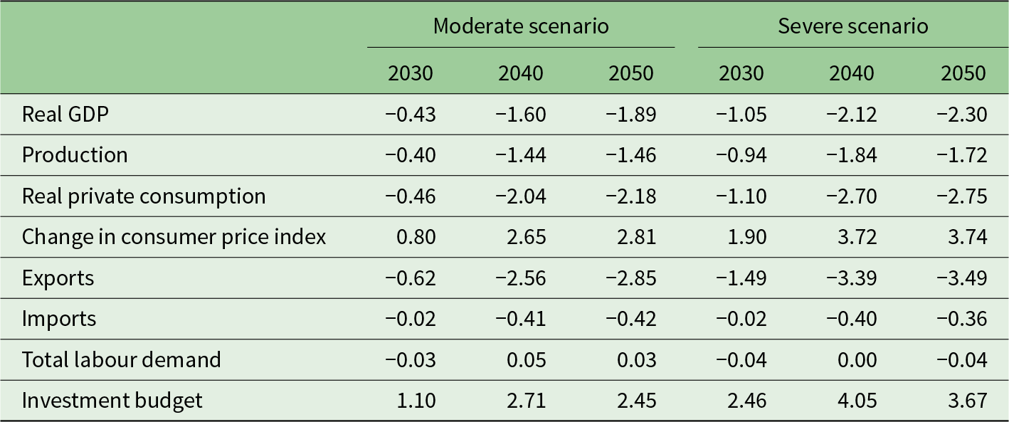
Table 2 Long description
The table compares percentage changes in macroeconomic indicators under moderate and severe scenarios for 2030, 2040, and 2050. Key findings include a consistent decline in GDP real, production, and exports, with the severe scenario showing larger decreases by 2050, such as a 2.30% drop in GDP real and a 3.49% drop in exports. Conversely, the investment budget increases, reaching 3.67% in the severe scenario by 2050. The consumer price index rises in both scenarios, with a more significant increase in the severe scenario, peaking at 3.74% in 2050. Imports and total labor demand show minimal changes, indicating relative stability in these areas. The data suggests that while economic output and trade suffer under severe conditions, investment remains robust, potentially indicating a shift in economic priorities.
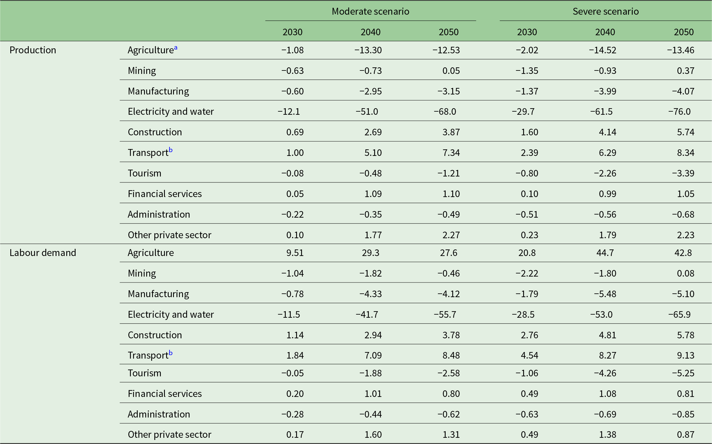
Table 3 reports the variations in production and labour demand, illustrating how the scenario affects different economic sectors. The sectors directly affected by climate change (agriculture, water and tourism) show reduced production, which impacts, on the one hand, their supply of intermediate commodities to other sectors (linked forward) and, on the other hand, their demand for commodities from other sectors (linked backward). Thus, interlinked sectors in the economy are indirectly impacted by the responses of the directly impacted sectors. For instance, in the moderate scenario in 2040, the water sector reduces its production by 51 per cent, which leads to an increase in the price of water by 13.7 per cent (see Appendix Table A1(c)). The price increase impacts all forward-linked sectors using water for production.
Impacts on production and labour demand (in % change to the BAU)

Table 3 Long description
The table measures percentage changes in production and labor demand across various sectors from 2030 to 2050 under moderate and severe scenarios. Electricity and water production faces the steepest decline, especially in the severe scenario, dropping by 76% by 2050. Conversely, construction and transport sectors show growth, with transport increasing by 8.34% in the severe scenario by 2050. Agriculture experiences significant labor demand increases, particularly in the severe scenario, with a 42.8% rise by 2050. Manufacturing and tourism sectors generally decline in both production and labor demand across all years and scenarios. The data includes fishery, forestry, trade, and communication sectors, which may influence these trends.
a Including fishery and forestry.
b Including trade and communication.
For the agricultural sector, the impact is quite interesting: on the one hand, the drop in productivity and capital depreciation reduces production and the intermediate consumption of products from backward-linked sectors. On the other hand, increased world agricultural prices accompany these negative impacts on production. In the short run, in 2030, South African producers even aim to export more agricultural products for higher prices, increasing production despite decreased productivity (Appendix Table A1(a)). The increasing world prices partially compensate for the losses of agricultural income from the impacts of climate change.
These sectoral production declines will have effects on employment, which declines by 0.03 per cent in 2030 (Table 2). The employment effects will vary depending on the sector and will not be uniform across categories of workers. For instance, the decrease in tourism spills over to the demand for services in hotels and restaurants. The tourism industry reduces production and fires workers, among whom women are highly represented and strongly impacted by the lay-offs. Unskilled male workers benefit from the positive impact on the construction and transport sectors, but suffer from the lay-offs in the manufacturing and water sectors. Indeed, as the investment budget increases (Table 2), the sectors that produce investment goods increase (e.g., construction). These sectors are intensive in unskilled male workers. The administration sector sees its production reducing, which will mainly impact skilled workers.
The change in the magnitude of the results between 2030 and subsequent years (2040, 2050) is explained by the fact that from 2030, we assume that the depreciation of capital in the agricultural and water sectors increases. Indeed, from 2030, for these two sectors, it becomes more expensive to maintain the existing capital stock, and therefore, the two sectors are much less attractive in terms of new investments. Consequently, production falls further.
Gender-differentiated labour market outcomes are driven by sectoral expansion and contraction and the reallocation of labour from shrinking sectors, reflecting the gender composition of employment. Male labour is concentrated in the primary and secondary sectors and in male-dominated services such as construction and transport. Women account for about half of service-sector employment but remain underrepresented in male-intensive activities. Contracting sectors, notably manufacturing, are male-dominated and primarily displace male workers; however, expanding sectors such as agriculture and transport are also male-dominated and absorb much of this displaced labour, resulting in a net increase in demand for male labour. In contrast, female-intensive sectors contract modestly, and no expanding sectors sufficiently absorb displaced female labour, leading to weaker labour market outcomes for women.
Overall, in 2030, the demand for male unskilled workers is increasing by 0.11 per cent, while that for unskilled female workers is decreasing by 0.12 per cent (Table 4). For skilled male workers, the demand remains stable, while that for skilled female workers drops by 0.08 per cent. Given the drop in labour demand in the paid market, unpaid work increases, particularly for women.
Impacts on labour demand by labour type (in % change to the BAU)

Table 4 Long description
The table measures percentage changes in labor demand by gender and skill level from the business-as-usual scenario for 2030, 2040, and 2050 under moderate and severe scenarios. Unskilled male labor demand increases in both scenarios, peaking at 0.52% in 2040 under severe conditions. Unskilled female labor demand decreases notably, with a severe drop to -0.66% in 2050 under severe scenarios. Skilled male labor demand shows slight increases, with the highest change of 0.09% in 2050 under moderate scenarios. Skilled female labor demand consistently declines, with the most significant drop of -0.21% in 2050 under severe scenarios. The data suggests that unskilled female labor is most negatively impacted, while skilled male labor experiences modest growth.
a Unskilled labour refers to men and women with no or primary school education.
b Skilled labour refers to men and women with secondary or higher school education.
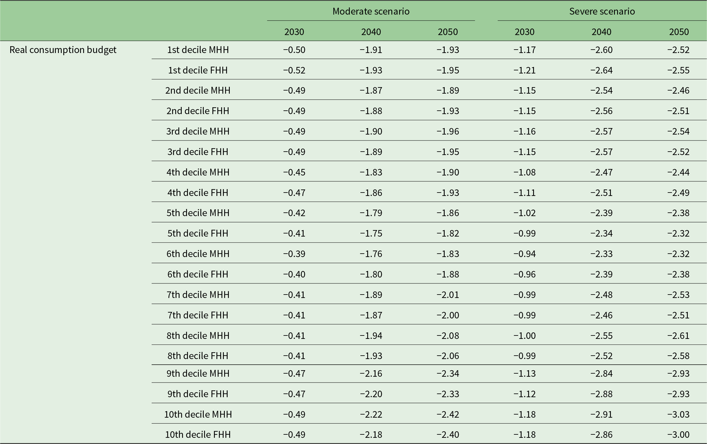
The depreciation of capital in the agricultural sector raises the price of capital and consequently increases the relative demand for labour as a production factor. Moreover, sectors that benefit from an increase in their production (construction and transport) also need more labour, particularly unskilled labour. As a result, the nominal wages for unskilled workers rise. The wage increase is higher for unskilled men than for women. Sectors where skilled women are intensive, see their production falling, and consequently, the wage rate for skilled women decreases. However, overall, the nominal income increases for each household. Nevertheless, the income increase is insufficient to compensate for the increase in consumer prices. Thus, households’ real consumption decreases despite increased income (Table 5).
Impacts on households’ real consumption (in % change to the BAU)

Table 5 Long description
The table measures the percentage change in real consumption for male-headed and female-headed households across different income deciles under moderate and severe scenarios from 2030 to 2050. In both scenarios, higher deciles generally experience larger decreases, with the 10th decile male-headed households seeing the largest drop of 3.03% in 2050 under the severe scenario. Female-headed households show similar trends, with slightly smaller decreases in some cases. The data suggests that severe scenarios have a more pronounced negative impact on real consumption across all deciles and household types. The differences between male-headed and female-headed households are minimal, indicating similar vulnerability to economic changes.
MHH, male-headed households; FHH, female-headed households.
4.2. Microeconomic impacts
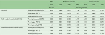
Table 6 presents the change in the poverty indicators for South Africa and the difference in changes between FHHs and MHHs. We compute the poverty indicators based on an upper-bound poverty line. The upper-bound poverty line indicates the benchmark above which households can purchase adequate food and non-food items. We orient the computation of the poverty indicators at the national level towards Stats SA (2018) and at the regional level towards Stats SA (2017b). The indicators show that FHHs are poorer than MHHs. The headcount, poverty gap and severity indicators are one and a half to two times higher for FHHs than for MHHs. As can be expected from the worsened economic conditions, the three poverty indicators increase for MHHs and FHHs. In the moderate scenario, the poverty headcount increases more than in the simulation year 2040. In the severe scenario, the increase exceeds more than 1 percentage point 10 years earlier, in 2030.
Change in poverty indicators in percentage points and the difference between female-headed households and male-headed households

Table 6 Long description
The table measures changes in poverty indicators from 2015 to 2050 under different scenarios, comparing national, male-headed, and female-headed households. In 2015, female-headed households had a higher poverty headcount at 49.9% compared to 33% for male-headed households. By 2050, under the severe scenario, the poverty headcount increases by 2.322 percentage points nationally, 2.258 for male-headed households, and 2.237 for female-headed households. The poverty gap and severity also show similar trends, with female-headed households consistently having higher values. The moderate scenario predicts smaller increases in poverty indicators compared to the severe scenario. These trends highlight the persistent disparity between male and female-headed households in poverty levels.
The regional economic and socio-economic differences cause heterogenous impacts on the poverty gaps between FHHs and MHHs. The Eastern Cape, KwaZulu-Natal, North West, Mpumalanga and Limpopo are among the poorest provinces, recording the highest poverty rates for FHHs (Stats SA, 2018). In these regions, the economy is dominated by the primary and secondary sectors, where women are either underrepresented or disadvantaged due to lower wages. Additionally, many of these provinces are rural, and many men migrate from the countryside to urban areas in search of better employment opportunities. Consequently, women are often left behind as household heads, carrying multiple responsibilities such as childcare, eldercare and managing subsistence farming or low-paid informal agricultural work.
In contrast, the economies of Gauteng and the Western Cape are largely driven by the tertiary sector, including tourism, finance and public administration. These sectors offer women greater access to employment opportunities with comparatively higher wages, resulting in lower poverty rates among FHHs. However, poverty hotspots still exist, particularly in informal urban settlements (e.g., townships located near major cities).
The Northern Cape and Free State provinces have the lowest population densities, and their economies are characterized by a significant contribution from primary and secondary activities, which together account for roughly one-third of economic output. The tertiary sector also provides employment opportunities for women, positioning these provinces between the extremes, those with highly tertiary-oriented economies (such as Gauteng and the Western Cape) and those dominated by mining and industrial activities (such as North West and Mpumalanga), in terms of poverty incidence among FHHs.
Figures 3a and b and 4a and b present the development of poverty gaps for the poverty incidence (FGT0) and poverty severity (FGT2). The colour indicates if the gaps between FHHs and MHHs widen (reddish) or narrow (blueish). The distributional pattern for poverty incidence and poverty severity is similar between the moderate and severe scenarios. Figure 3a and b shows that the poverty incidence gap widens in the reddish-coloured provinces of Northern Cape, Western Cape and Gauteng. This means that in the scenarios, the poverty headcount (FGT0) worsens more for women than for men. In provinces with higher poverty incidences in the reference scenario, the poverty gaps tend to decrease. In these provinces, so many MHHs and FHHs fall under the poverty line that, in the scenarios, more MHHs than FHHs tend to fall. However, since the poverty incidence is high, increasing the development in total is still negative. The fact that climate change scenarios create a gender-gap-reducing effect could be interpreted as showing that in these already poor regions, policy instruments could be effectively applied to reduce the gender gaps.
Difference in changes in the poverty headcount index (FGT0), computed as the change in FHHs minus the change in MHHs, in (a) the moderate scenario in 2040 and (b) the severe scenario in 2040.

Figure 3 Long description
Both maps use a color gradient to indicate changes, with reddish tones showing an increase and blueish tones showing a decrease. Key regions such as Northern Cape, Western Cape and Gauteng are highlighted, with varying degrees of change in poverty incidence across the provinces.
Difference in changes in the poverty severity index (FGT2), computed as the change in FHHs minus the change in MHHs, in (a) the moderate scenario in 2040 and (b) the severe scenario in 2040.

Figure 4 Long description
The image shows two maps of South Africa labeled (a) and (b). Both maps depict changes in the poverty severity index (FGT2) for different provinces. Map (a) represents the moderate scenario in 2040, while map (b) represents the severe scenario in 2040. The color gradient indicates the change, with darker shades representing greater changes. Provinces such as Limpopo, Mpumalanga and KwaZulu-Natal show significant changes. The maps include labels for provinces and major cities like Johannesburg and Cape Town.
Figure 4a and b presents the regional difference in changes for the poverty severity indicator (FGT2). In all provinces, the impact on poverty severity (FGT2) is stronger for women than for men, particularly in some provinces with higher poverty incidence. In Gauteng, the impact is less strong. In the larger cities of Johannesburg and Pretoria, the job and income opportunities and financial support for poor households might be higher than in other, more rural provinces. More income opportunities and financial support explain a buffering effect for worsening poverty in Gauteng. Also, the number of FHHs is lower in Gauteng than in rural provinces, where women are often left behind by men migrating for better jobs in mining or industry. The interpretation of the regional results requires attention since we simulated the climate change shocks at the country level and translated them into the distributional analysis at the household and regional levels. Since climate change shocks are regionally heterogeneous, a more consistent analysis would require the simulation of the impacts of climate change at the regional level.
5. Conclusions
The nexus between climate change and gender is complex, and the sector-specific impacts on the socio-economic situation are difficult to understand. Designing effective and efficient counteracting policies against climate change impacts requires assessment through the gender lens, considering time allocation between work in the labour market and domestic responsibilities. The results indicate, in a moderate scenario of climate change, a 1.9 per cent decrease in GDP. Paid labour decreases, especially for women, and unpaid labour increases for all categories of households. The nominal income increases, but a high increase in consumer prices negatively affects the consumption of all households. Therefore, at the household level, poverty increases, especially for the poorest women. The results are even more dramatic in the severe scenario where the demand for work is reduced, and the poverty of the poorest women increases very significantly.
Beyond its methodological contribution, our analysis also carries important policy implications. The differentiated gender impacts of climate change highlighted here underline the need for targeted social protection, particularly for women concentrated in vulnerable sectors such as agriculture and tourism. This targeting could combine compensatory transfers (in cash or in kind) with investments in education and training that enhance women’s access to more resilient activities. Also, investing in women’s access to productive resources such as land and credit will enhance long-term resilience and contribute to sustainable economic recovery.
Specific sectoral aids could address multiple problems at the same time. Investment in climate-adapted technologies and production systems in agriculture could compensate for climate-induced losses (e.g., climate-smart agriculture). The tourism sector requires adaptation measures and investment in infrastructure to counteract the impacts of climate change and the decrease in tourism demand. In agriculture and tourism, labour market policies can strengthen women's position and reduce gender gaps (e.g., in salary). In general, many pro-gender and pro-poor policies can support the adaptive capacities of individuals and families. Providing infrastructure and services to households to overcome domestic burdens (childcare, electrification) can enhance women's economic opportunities, enrich the labour market and foster economic growth.
As an economy-wide assessment, we analyse sectors at a highly aggregated level. Information on climate-sensitive subsectors (e.g., specific crop sectors in agriculture or tourism) is required to design sector-specific policies. The CGE model simulations and results are at the country level. Regional climatic and geographic conditions and socio-economic conditions strongly determine climate and economic impacts. Thus, an analysis considering regional heterogeneity would provide more reliable results. Finally, we derive the climate impact scenarios based on studies and combine them into moderate and severe impact scenarios. However, these scenarios represent only rough benchmarks to define a scenario space. The results can be interpreted only within this rough scenario space.
In future research, simulations and analyses should overcome these limitations. Further modelling work could provide more differentiated sectors and scenarios and consider a higher regional resolution, as well as including impacts on children and the elderly. To obtain modelling results, the CGE model might be linked to and extended by other models, as already applied in climate change research. Here, the consideration of the gendered dimension would be of interest, particularly for socio-economic models. Better modelling of domestic chores helps show the direct impacts of climate change on the female labour force and women’s working time. The essential requirements are a survey of more empirically founded data, which can be used to better calibrate and validate policy simulation models. Based on better empirical data, domestic chores can be better disaggregated in the model. They can be used to analyse further macroeconomic and microeconomic aspects and gendered aspects of policy instruments and economic shocks. Thus, accompanying empirical studies can support parameter estimation and validate the model results. A research framework coordinating directly with policy stakeholders could foster the production of policy-relevant results and make the information directly accessible for policy decisions.
The pure economic model-based study presented cannot provide concrete solutions to the problem of the gendered impacts of climate change. Too many assumptions determine the results, and the model can cover only a few aspects. However, this study can contribute in a way that model-based studies can do. Suspected and empirically observed problems can be simulated at a macroeconomic scale, and the economic mechanisms can be shown. Thus, the results can enter the debate for further discussion and as an incentive for the development of research to fight the impacts of climate change in a manner that addresses gender equity.
Supplementary material
The supplementary material for this article can be found at https://doi.org/10.1017/S1355770X26100588.
Competing interest
None for both authors.