1. Introduction
When a steady flow becomes linearly unstable owing to the variation of a control parameter, a bifurcation process occurs due to the inherent nonlinearity of the governing Navier–Stokes equations. As a result of this process, a new flow state develops, either steady or unsteady, being usually characterized by an inferior degree of symmetry with respect to the basic state. Classical examples are represented by the flow between rotating cylinders (Taylor–Couette flow), convection in a fluid layer heated from below (Rayleigh–Bérnard–Marangoni flow) and by the flow past a bluff body such as a circular cylinder or a sphere. In the simplest case, when the flow instability is driven by a single global mode, relevant information concerning the frequency and the spatial pattern of the emerging flow state can be deduced from a linear stability analysis. However, when two or more linear modes become unstable for the same values of the control parameters, neither stability nor pattern selection can be completely explained based solely on the linear approach. Such a condition, which corresponds to the occurrence of multiple codimension bifurcations, has been found to characterize several flow configurations (Rehberg & Ahlers Reference Rehberg and Ahlers1985; Tuckerman Reference Tuckerman2001; Marques, Lopez & Shen Reference Marques, Lopez and Shen2002; Meliga, Gallaire & Chomaz Reference Meliga, Gallaire and Chomaz2012; Marques, Mellibovsky & Meseguer Reference Marques, Mellibovsky and Meseguer2013; Tchoufag, Fabre & Magnaudet Reference Tchoufag, Fabre and Magnaudet2014).
Within the framework of nonlinear dynamical systems, the problem of mode selection among competing instabilities can be tackled by means of the centre-manifold approximation of the nonlinear dynamics (Charru Reference Charru2011). In fact, it is well known that in the neighbourhood of the bifurcation of a fixed equilibrium, the essential dynamics is determined only by those modes which are marginally stable in the linearized description, i.e. the critical modes. If all of the remaining modes are stable and heavily damped, the state of the nonlinear system rapidly converges onto a low-dimensional, attractive and invariant manifold in the phase space, the centre manifold (Guckenheimer & Holmes Reference Guckenheimer and Holmes1983; Haragus & Iooss Reference Haragus and Iooss2011). Once the original system has been reduced to a centre manifold, the description of the dynamics can be further simplified to its normal form while preserving its structural properties. This reduction allows one to deduce relevant information of the system behaviour based on the general normal-form theory and classification. For several physical systems, the normal form structure can also be deduced a priori from symmetry considerations, making use of the theory of groups (Crawford & Knobloch Reference Crawford and Knobloch1991).
Different methods have been described in the literature to build an approximation to the centre manifold and to reduce it to its normal form, the two operations being often treated as two successive distinct steps. Basically the various techniques can be divided in two main classes, with respect to the computation of the centre manifold (Kuznetsov Reference Kuznetsov1998). Methods of the first class require the explicit computation of all of the eigenvalues and eigenfunctions associated with the linearized vector field in order to change the natural system state basis into the eigenbasis. This requirement makes such techniques unaffordable for large-scale applications where the computation of the whole spectrum of the linearized operator is prohibitively expensive. In contrast, methods of the second class rely on the projection of the nonlinear state onto the critical subspace. Hence, only direct and adjoint critical linear modes are needed: for typical applications, a small number of such modes is present, thus making the latter approach suitable for high-dimensional dynamical systems.
The projection approach lies at the heart of the method described by Coullet & Spiegel (Reference Coullet and Spiegel1983) and of that of multiple time-scales which has been used for a long time in the field of hydrodynamic stability (Stuart Reference Stuart1971). In both cases, the centre-manifold reduction and the normal-form computation are obtained within a single step, thus avoiding the introduction of near-identity nonlinear transformations, usually involved in the derivation of the normal form (Charru Reference Charru2011). Based on the common framework of asymptotic expansions, the flow state in the neighbourhood of the critical threshold is approximated in power series of the bifurcation parameter and of the renormalized critical mode amplitudes, the involved expansion procedure being handled manually. Although on the one hand this can provide additional physical insight by granting access step by step to the individual terms of the expansion and to their dependence from low-order ones, on the other hand, however, this approach becomes quite cumbersome at increasing orders of the approximation, especially in the case of high-codimension bifurcations.
The aim of this paper is to illustrate a different technique with respect to that of multiple scales to perform the weakly nonlinear analysis of bifurcating flows within a global setting (Sipp & Lebedev Reference Sipp and Lebedev2007; Meliga et al. Reference Meliga, Gallaire and Chomaz2012). Compared with the method of multiple scales, the proposed technique has the main advantage that it can be fully automated by means of numerical computations in a rather general way and for an arbitrary dimension of the critical subspace. Moreover, the additional complications associated with the introduction of a slow time scale to separate the motion onto the centre manifold from the fast-decaying stable dynamics are avoided. For such purpose, the approach described by Coullet & Spiegel (Reference Coullet and Spiegel1983) is recast into a formulation which can be coded directly into a computer algorithm, without any need to resort to symbolic computation. Then the method is applied to two examples of bifurcating flows. In the first, the onset of the cylinder vortex shedding is considered, for which both the normal-form (Landau) coefficients and the related nonlinear global modes have been computed by various authors (Sipp & Lebedev Reference Sipp and Lebedev2007; Meliga & Chomaz Reference Meliga and Chomaz2011). In the second, the codimension-two pitchfork-Hopf bifurcation which characterizes the flow past two side-by-side circular cylinders is examined.
The paper is organized as follows. First, a brief reminder of the centre-manifold and normal-form theory for finite-dimensional dynamical systems is given in § 2. In § 3 the centre-manifold reduction is introduced within an abstract, general framework and a simple low-dimensional example is illustrated in § 3.2. The application to the incompressible Navier–Stokes equations is discussed in § 4 and results obtained for the above-mentioned flow configurations are described in §§ 4.2 and 4.3. Finally a summary of the work is given in § 5.
2. Centre manifold and normal form: a brief review
Let us consider the generic autonomous finite-dimensional dynamical system
 $$\begin{eqnarray}\dot{\boldsymbol{q}}=\boldsymbol{F}(\boldsymbol{q}),\end{eqnarray}$$
with
 $\boldsymbol{q}(t)\in \mathbb{R}^{n}$
and a related fixed point
 $\boldsymbol{q}_{0}$
, i.e.
 $\boldsymbol{F}(\boldsymbol{q}_{0})=\mathbf{0}$
. Without loss of generality we can assume that
 $\boldsymbol{q}_{0}=\mathbf{0}$
. The nature of the fixed point
 $\boldsymbol{q}_{0}$
depends on the stability of the linearized vector field around it
 $$\begin{eqnarray}\dot{\boldsymbol{q}}=\unicode[STIX]{x1D647}\boldsymbol{q},\end{eqnarray}$$
where
 $\unicode[STIX]{x1D647}$
denotes the Jacobian of
 $\boldsymbol{F}$
evaluated for
 $\boldsymbol{q}=\boldsymbol{q}_{0}$
. Denoting with
 ${\it\Lambda}(\unicode[STIX]{x1D647})$
the spectrum of
 $\unicode[STIX]{x1D647}$
,
 $\boldsymbol{q}_{0}$
is called hyperbolic if
 $\text{Re}({\it\lambda})\neq 0,\forall {\it\lambda}\in {\it\Lambda}(\unicode[STIX]{x1D647})$
. Hence, in the hyperbolic case no marginally stable modes exist and the local stability of
 $\boldsymbol{q}_{0}$
follows from that of the linearized system (2.2).
For a non-hyperbolic fixed point at least one eigenmode of
 $\unicode[STIX]{x1D647}$
is found to be critical and the invariant subspace
 $E^{c}$
spanned by those eigenmodes which are marginally stable is referred to as the critical or centre subspace. In this case it can be proved that an invariant smooth manifold
 ${\mathcal{V}}^{c}$
also exists in the phase–space which has the same dimension of
 $E^{c}$
, the centre manifold. The centre manifold theory is of particular interest when all the eigenvalues of
 $\unicode[STIX]{x1D647}$
are stable except those lying on the imaginary axis. In such a condition the local stability of
 $\boldsymbol{q}_{0}$
cannot be deduced from that of the linearized system (2.2). At the same time it can be shown that starting from any given initial condition, the trajectories of the nonlinear system asymptotically approach the centre manifold (Guckenheimer & Holmes Reference Guckenheimer and Holmes1983). Therefore, the centre-manifold approximation of the nonlinear dynamics naturally provides a low-dimensional description of its asymptotic behaviour in a neighbourhood of
 $\boldsymbol{q}_{0}$
. To better explain this point let us rewrite the system (2.1) as follows:
 $$\begin{eqnarray}\left.\begin{array}{@{}c@{}}\dot{\boldsymbol{q}}_{c}=\unicode[STIX]{x1D647}_{c}\boldsymbol{q}_{c}+\boldsymbol{f}_{c}(\boldsymbol{q}_{s},\boldsymbol{q}_{c}),\\ \dot{\boldsymbol{q}}_{s}=\unicode[STIX]{x1D647}_{s}\boldsymbol{q}_{s}+\boldsymbol{f}_{s}(\boldsymbol{q}_{s},\boldsymbol{q}_{c}),\end{array}\right\}\end{eqnarray}$$
where
 $\boldsymbol{q}_{c}(t)\in \mathbb{R}^{n_{c}}$
and
 $\boldsymbol{q}_{s}(t)\in \mathbb{R}^{n-n_{c}}$
,
 $n_{c}$
being the dimension of the critical subspace. As already mentioned, usually
 $n_{c}\ll n$
for large-scale systems. The above formulation is simply derived from the decomposition of
 $\boldsymbol{F}(\boldsymbol{q})$
into its linear and nonlinear part, i.e.
 $\boldsymbol{F}(\boldsymbol{q})=\unicode[STIX]{x1D647}\boldsymbol{q}+\boldsymbol{f}(\boldsymbol{q})$
followed by a linear coordinate transformation in the eigenbasis of
 $\unicode[STIX]{x1D647}$
. This latter transformation allows
 $\boldsymbol{q}$
to be partitioned according to the invariant subspaces
 $E^{c}$
and
 $E^{s}$
, where
 $E^{s}$
denotes the subspace spanned by the stable modes of
 $\unicode[STIX]{x1D647}$
, i.e. its stable subspace. Correspondingly the spectrum of
 $\unicode[STIX]{x1D647}_{c}$
lies on the imaginary axis while all of the eigenvalues of
 $\unicode[STIX]{x1D647}_{s}$
have strictly negative real part. The nonlinear functions
 $\boldsymbol{f}_{c}$
and
 $\boldsymbol{f}_{s}$
are assumed to be smooth and at least quadratic near the origin, i.e. in the neighbourhood of
 $\boldsymbol{q}_{0}$
. Under these assumptions, the centre-manifold theorem guarantees the existence of a smooth
 $n_{c}$
-dimensional manifold which can be represented as a map
 $\tilde{\boldsymbol{q}}_{s}=\boldsymbol{{\it\Upsilon}}(\tilde{\boldsymbol{q}}_{c})$
from
 $E^{c}$
to
 $E^{s}$
and which is tangent to
 $E^{c}$
at the origin, i.e. at the fixed point
 $\boldsymbol{q}_{0}$
(Guckenheimer & Holmes Reference Guckenheimer and Holmes1983). It is worthwhile to remember that if
 $\boldsymbol{F}(\boldsymbol{q})$
belongs to the class
 $\mathscr{C}^{r}$
,
 ${\mathcal{V}}^{c}$
belongs only to the class
 $\mathscr{C}^{r-1}$
. In addition
 ${\mathcal{V}}^{c}$
is not necessarily unique (Guckenheimer & Holmes Reference Guckenheimer and Holmes1983, p. 124). More precisely, if more than one centre manifold exists with different maps
 $\boldsymbol{{\it\Upsilon}}$
, all of the resulting reduced-order systems are topologically equivalent in the neighbourhood of
 $\boldsymbol{q}_{0}$
(Kuznetsov Reference Kuznetsov1998). Therefore, in our discussion we will refer to ‘the’ centre manifold rather than to ‘a’ centre manifold. Finally, as reported by Roberts (Reference Roberts1997), the computation of the centre-manifold reduction relies on the so-called approximation theorem which guarantees that the map
 $\boldsymbol{{\it\Upsilon}}$
can be approximated up to the same order of accuracy at which (2.1) is satisfied.
Once the map
 $\tilde{\boldsymbol{q}}_{s}=\boldsymbol{{\it\Upsilon}}(\tilde{\boldsymbol{q}}_{c})$
has been introduced, the system dynamics onto
 ${\mathcal{V}}^{c}$
is described by the low-dimensional system:
 $$\begin{eqnarray}\dot{\tilde{\boldsymbol{q}}}_{c}=\unicode[STIX]{x1D647}_{c}\tilde{\boldsymbol{q}}_{c}+\boldsymbol{f}_{c}(\boldsymbol{{\it\Upsilon}}(\tilde{\boldsymbol{q}}_{c}),\tilde{\boldsymbol{q}}_{c}).\end{eqnarray}$$
These equations are often referred to as the amplitude equations (Coullet & Spiegel Reference Coullet and Spiegel1983). When applied to the above set of equations, the derivation of the normal form provides the simplest parametrization of the motion of the system onto the centre manifold. Starting from (2.4), the normal-form computation usually involves a sequence of near-identity nonlinear transformations needed to eliminate as many nonlinear terms as possible from
 $\boldsymbol{f}_{c}(\boldsymbol{{\it\Upsilon}}(\tilde{\boldsymbol{q}}_{c}),\tilde{\boldsymbol{q}}_{c})$
up to a selected finite order while preserving the linear part
 $\unicode[STIX]{x1D647}_{c}$
. Of course, some nonlinear terms cannot be eliminated by any coordinate change: these terms which rule the asymptotic behaviour of the system dynamics are usually referred to as resonant terms. Indeed, as it will be made clear in the description of the proposed method, these irreducible nonlinearities are associated with the forced harmonic response
 $\boldsymbol{q}(t)=\hat{\boldsymbol{q}}_{{\it\omega}_{c}}\text{e}^{\imath {\it\omega}_{c}t}$
of the linearized system at one of its critical frequencies:
 $$\begin{eqnarray}(\unicode[STIX]{x1D647}-\imath {\it\omega}_{c}\unicode[STIX]{x1D644})\hat{\boldsymbol{q}}_{{\it\omega}_{c}}=\hat{\boldsymbol{h}}_{{\it\omega}_{c}},\end{eqnarray}$$
where the harmonic forcing
 $\hat{\boldsymbol{h}}_{{\it\omega}_{c}}$
arises from the nonlinear-mode interaction,
 $\unicode[STIX]{x1D644}\in \mathbb{R}^{n\times n}$
denotes the identity matrix and
 $\imath {\it\omega}_{c}\in {\it\Lambda}(\unicode[STIX]{x1D647}_{c})$
. To avoid confusion with the integer index
 $i$
, in this paper the imaginary unit is denoted by the special character
 $\imath$
. The special case of a steady critical mode simply corresponds to
 ${\it\omega}_{c}=0$
. Note that
 $\unicode[STIX]{x1D647}-\imath {\it\omega}_{c}\unicode[STIX]{x1D644}$
is singular by definition which expresses the resonance condition. Therefore to compute
 $\hat{\boldsymbol{q}}_{{\it\omega}_{c}}$
, the Fredholm solvability condition must be enforced by introducing additional degrees of freedom which are shown to correspond to the normal form coefficients. A complete and rigorous discussion on this point can be found in the theoretical work by Coullet & Spiegel (Reference Coullet and Spiegel1983) and Elphick et al. (Reference Elphick, Tirapegui, Brachet, Coullet and Iooss1987).
It should be noted that the computation of high-order normal forms can exploit several techniques which focus on the automatic and efficient handling of the sequence of involved nonlinear transformations, see e.g. Zhang, Huseyin & Ye (Reference Zhang, Huseyin and Ye2000), Hsu, Min & Favretto (Reference Hsu, Min and Favretto2001) and Yu & Yuan (Reference Yu and Yuan2003). However, the description of such techniques is beyond the scope of our discussion since, as already mentioned in § 1, the proposed method allows one to derive directly the amplitude equations in their normal form.
3. Centre-manifold reduction
In this section the proposed centre-manifold reduction technique is described in detail. With respect to the classical approach mentioned in § 2, the present method allows the computation of the centre-manifold reduction in its normal form just within a single step, without introducing any coordinate transformation in the eigenbasis of
 $\unicode[STIX]{x1D647}$
. Instead, only the knowledge of the critical subspace is required in order to project the system dynamics onto
 $E^{c}$
and its orthogonal complement
 $E^{s}$
(Kuznetsov Reference Kuznetsov1998), thus enabling the treatment of large-scale systems.
Let us consider the nonlinear dynamical system (2.1) where the dependency on a real control parameter
 ${\it\epsilon}$
is introduced. In addition, for the sake of generality, we rewrite (2.1) in the generalized form
 $$\begin{eqnarray}\unicode[STIX]{x1D63D}\dot{\boldsymbol{q}}=\boldsymbol{F}(\boldsymbol{q},{\it\epsilon}),\end{eqnarray}$$
where
 $\unicode[STIX]{x1D63D}$
can be singular such as for the discretized incompressible Navier–Stokes system in primitive variables. Splitting the nonlinear operator
 $\boldsymbol{F}$
into the linear part
 $\unicode[STIX]{x1D647}$
and nonlinear part
 $\boldsymbol{f}(\boldsymbol{q},{\it\epsilon})$
yields
 $$\begin{eqnarray}\unicode[STIX]{x1D63D}\dot{\boldsymbol{q}}=\unicode[STIX]{x1D647}\boldsymbol{q}+\boldsymbol{f}(\boldsymbol{q},{\it\epsilon}),\end{eqnarray}$$
where, under the assumptions introduced in § 2,
 $\boldsymbol{f}(\mathbf{0},0)=\mathbf{0}$
. Note that the, possibly nonlinear, dependence on
 ${\it\epsilon}$
is accounted for in
 $\boldsymbol{f}$
. Here the description of the method is limited to the case of
 $\unicode[STIX]{x1D647}$
being diagonalizable although an extension to the non-diagonalizable case is possible. In the neighbourhood of the fixed non-hyperbolic point
 $\boldsymbol{q}_{0}=\mathbf{0}$
we known that the system dynamics asymptotically evolves on the centre manifold whose dimension is equal to the dimension
 $n_{c}$
of the critical subspace. Therefore, we can express
 $\boldsymbol{q}(t)$
as a function of a reduced system state
 $\boldsymbol{a}(t)=(a_{1}(t),a_{2}(t),\dots ,a_{n_{c}}(t))$
and of the bifurcation parameter
 ${\it\epsilon}$
 $$\begin{eqnarray}\boldsymbol{q}(t)=\boldsymbol{q}(\boldsymbol{a}(t),{\it\epsilon}).\end{eqnarray}$$
The components
 $a_{\ell }$
of
 $\boldsymbol{a}$
are called critical amplitudes and can be interpreted as generalized coordinates describing the motion of the dynamical system on the centre manifold which is ruled by the low-dimensional nonlinear equation
 $$\begin{eqnarray}\dot{\boldsymbol{a}}=\boldsymbol{g}(\boldsymbol{a}(t),{\it\epsilon}).\end{eqnarray}$$
By virtue of the centre-manifold approximation theorem and based on the approach proposed by Coullet & Spiegel (Reference Coullet and Spiegel1983), we can then approximate the system dynamics using the method of asymptotic expansions. In the neighbourhood of
 $\boldsymbol{q}_{0}$
, both
 $\boldsymbol{q}(\boldsymbol{a}(t),{\it\epsilon})$
and
 $\boldsymbol{g}(\boldsymbol{a}(t),{\it\epsilon})$
are expanded as infinite power series of
 $a_{\ell }(t)$
and
 ${\it\epsilon}$
,
 $$\begin{eqnarray}\displaystyle \boldsymbol{q}(t)=\mathop{\sum }_{m=1}^{\infty }\mathop{\sum }_{|\boldsymbol{i}|+k=m}\hat{\boldsymbol{q}}_{\boldsymbol{i},k}\,\boldsymbol{a}^{\boldsymbol{i}}(t){\it\epsilon}^{k}, & & \displaystyle\end{eqnarray}$$
 $$\begin{eqnarray}\displaystyle \boldsymbol{g}(\boldsymbol{a}(t),{\it\epsilon})=\mathop{\sum }_{m=1}^{\infty }\mathop{\sum }_{|\boldsymbol{i}|+k=m}\hat{\boldsymbol{g}}_{\boldsymbol{i},k}\,\boldsymbol{a}^{\boldsymbol{i}}(t){\it\epsilon}^{k}, & & \displaystyle\end{eqnarray}$$
 $\boldsymbol{i}=(i_{1},i_{2},\dots \,,i_{n_{c}})$
is a multi-index of
 $n_{c}$
integers with
 $|\boldsymbol{i}|=\sum _{\ell =1}^{n_{c}}i_{\ell }$
and
 $\boldsymbol{a}$
is raised to
 $\boldsymbol{i}$
th power according to
 $$\begin{eqnarray}\boldsymbol{a}^{\boldsymbol{i}}\equiv \mathop{\prod }_{\ell =1}^{n_{c}}a_{\ell }^{i_{\ell }}.\end{eqnarray}$$
In (3.5) the vector-valued coefficients
 $\hat{\boldsymbol{q}}_{\boldsymbol{i},k}$
represent the generalized nonlinear modes which allow one to recover the full system state starting from the reduced state
 $\boldsymbol{a}(t)$
. Once the unknown expansion coefficients
 $\hat{\boldsymbol{q}}_{\boldsymbol{i},k}$
and
 $\hat{\boldsymbol{g}}_{\boldsymbol{i},k}$
have been determined, the time evolution of dynamical system (3.1) on the centre manifold is obtained first by solving (3.4) and then reconstructing
 $\boldsymbol{q}(t)$
using (3.5). Although different notation could be used to handle the expansions in (3.5) and (3.6), the compact one adopted here is particularly convenient since terms of equal order
 $m=|\boldsymbol{m}|+p$
are collected together. We note in passing that, while in the multiple-scale formalism an expansion in powers of the
 ${\it\epsilon}$
is first assumed, with the expansion in the critical amplitudes being derived by construction (Charru Reference Charru2011, p. 251), in the centre-manifold approximation formalism (Coullet & Spiegel Reference Coullet and Spiegel1983; Elphick et al.
Reference Elphick, Tirapegui, Brachet, Coullet and Iooss1987), the solution is expanded in polynomial series of both the parameter and the critical amplitudes ab initio. It should also be noted that the amplitudes have a slightly different meaning in the two formalisms, as shown in § 4.2.
In order to compute the expansion coefficients
 $\hat{\boldsymbol{q}}_{\boldsymbol{i},k}$
and
 $\hat{\boldsymbol{g}}_{\boldsymbol{i},k}$
, the expressions (3.5) and (3.6) are introduced in (3.1) and the terms with the same indices
 $(\boldsymbol{i},k)$
are collected, thus equating the coefficients of all similar monomials
 $a_{1}^{i_{1}}\dots \,a_{n_{c}}^{i_{n_{c}}}{\it\epsilon}^{k}$
. As will be made clear later on, this procedure leads to the solution of a sequence of linear systems which correspond to the forced harmonic response of the linearized dynamics to nonlinear interactions
 $$\begin{eqnarray}(\unicode[STIX]{x1D647}-\imath {\it\omega}\unicode[STIX]{x1D63D})\hat{\boldsymbol{q}}_{{\it\omega}}=\hat{\boldsymbol{h}}_{{\it\omega}}.\end{eqnarray}$$
When the forcing occurs at one of the critical frequencies, a resonant term of the expansions is generated. As already mentioned in § 2, only these terms contribute to the normal form and therefore only the related coefficients
 $\hat{\boldsymbol{g}}_{\boldsymbol{i},k}$
in (3.6) are different from zero, providing the required degrees of freedom to enforce the solvability condition for the resonant linear systems (2.5).
3.1. Reduction procedure
The above introduced expansions for
 $\boldsymbol{q}(\boldsymbol{a},{\it\epsilon})$
and
 $\boldsymbol{g}(\boldsymbol{a},{\it\epsilon})$
are now truncated up to a selected finite degree
 $\bar{r}=|\boldsymbol{i}|+p$
to address the problem numerically. The number of terms of fixed degree
 $m=|\boldsymbol{i}|+p$
is expressed by the binomial fraction
 $n_{m}=\binom{n_{c}+m}{n_{c}}$
. Then the total number of terms up to the truncation order
 $\bar{r}$
is
 $n_{t}=\sum _{m=1}^{\bar{r}}n_{m}$
.
By introducing (3.5) and (3.6) in (3.1) we obtain for the generic term
 $(\boldsymbol{m},p)$
 $$\begin{eqnarray}\left\langle \unicode[STIX]{x1D63D}\mathop{\sum }_{m=1}^{\bar{r}}\mathop{\sum }_{|\boldsymbol{i}|+k=m}\hat{\boldsymbol{q}}_{\boldsymbol{i},k}\dot{(\boldsymbol{a}^{\boldsymbol{i}})}{\it\epsilon}^{k}\right\rangle _{\boldsymbol{m},p}=\unicode[STIX]{x1D647}\hat{\boldsymbol{q}}_{\boldsymbol{m},p}+\langle \,\boldsymbol{f}(\boldsymbol{q}(\boldsymbol{a},{\it\epsilon}),{\it\epsilon})\rangle _{\boldsymbol{m},p},\end{eqnarray}$$
where the notation
 $\langle \boldsymbol{w}(\boldsymbol{a},{\it\epsilon})\rangle _{\boldsymbol{m},p}$
stands for the vector coefficient of the
 $(\boldsymbol{m},p)$
th term in the power series expansion of
 $\boldsymbol{w}(\boldsymbol{a},{\it\epsilon})$
. For a wide class of finite-dimensional dynamical systems, including many of those derived from the numerical discretization of partial differential equations (PDEs), the dependency of
 $\boldsymbol{f}$
on both
 $\boldsymbol{q}$
and
 ${\it\epsilon}$
is exactly expressed in algebraic form by means of multivariate polynomials (usually of small degree) in the components of
 $\boldsymbol{q}$
and in
 ${\it\epsilon}$
. More generally in the case of transcendent functions, an approximate algebraic expression for
 $\boldsymbol{f}(\boldsymbol{q},{\it\epsilon})$
can be derived by expanding in Taylor series in the neighbourhood of
 $\boldsymbol{q}=\mathbf{0}$
and
 ${\it\epsilon}=0$
. As an example, for a generic quadratic nonlinearity we can write
 $$\begin{eqnarray}\{\,\boldsymbol{f}(q_{1},\dots ,q_{n},{\it\epsilon})\}_{i}=\unicode[STIX]{x1D608}_{i}{\it\epsilon}+\unicode[STIX]{x1D609}_{ij}q_{j}{\it\epsilon}+\unicode[STIX]{x1D60A}_{ijk}q_{j}q_{k}+\unicode[STIX]{x1D60B}_{i}{\it\epsilon}^{2},\end{eqnarray}$$
where the Einstein summation convention has been used along with the notation
 $\{\boldsymbol{w}\}_{i}=w_{i}$
for the
 $i$
th component of the vector
 $\boldsymbol{w}$
. By substituting (3.5) in (3.10), the corresponding power series of
 $\boldsymbol{f}(\boldsymbol{q},{\it\epsilon})$
in the critical amplitudes and in
 ${\it\epsilon}$
is easily derived:
 $$\begin{eqnarray}\{\,\hat{\boldsymbol{f}}_{\boldsymbol{m},p}\}_{i}={\it\delta}_{\begin{array}{@{}c@{}}\boldsymbol{m},0\\ p,1\end{array}}\unicode[STIX]{x1D608}_{i}+{\it\delta}_{\begin{array}{@{}c@{}}\boldsymbol{m},0\\ p,2\end{array}}\unicode[STIX]{x1D60B}_{i}+\{\,\hat{\boldsymbol{f}}_{\boldsymbol{m},p}^{({\it\epsilon})}\}_{i}+\mathop{\sum }_{\begin{array}{@{}c@{}}\boldsymbol{i}+\boldsymbol{n}=\boldsymbol{m}\\ q+k=p\end{array}}\unicode[STIX]{x1D60A}_{ij\ell }\{\hat{\boldsymbol{q}}_{\boldsymbol{i},q}\}_{j}\{\hat{\boldsymbol{q}}_{\boldsymbol{n},k}\}_{\ell },\end{eqnarray}$$
where
 $$\begin{eqnarray}\{\,\hat{\boldsymbol{f}}_{\boldsymbol{m},p}^{({\it\epsilon})}\}_{i}=\left\{\begin{array}{@{}ll@{}}0\quad & \text{for}~p=0,\\ \unicode[STIX]{x1D609}_{ij}\{\hat{\boldsymbol{q}}_{\boldsymbol{m},p-1}\}_{j}\quad & \text{for}~p\geqslant 1,\end{array}\right.\end{eqnarray}$$
and
 $$\begin{eqnarray}{\it\delta}_{\begin{array}{@{}c@{}}\boldsymbol{m},\boldsymbol{i}\\ p,k\end{array}}=\left\{\begin{array}{@{}ll@{}}1\quad & \text{for}~(\boldsymbol{m},p)=(\boldsymbol{i},k),\\ 0\quad & \text{otherwise}.\end{array}\right.\end{eqnarray}$$
It can be observed that no coupling among terms of the same degree can arise due to the nonlinear term, since
 $\boldsymbol{f}$
is assumed to be at least quadratic in the neighbourhood of the origin.
At this point, in order to reduce (3.9) to a pure algebraic linear problem, time derivatives
 $\dot{(\boldsymbol{a}^{\boldsymbol{i}})}$
are expressed using the chain rule
 $$\begin{eqnarray}\dot{(\boldsymbol{a}^{\boldsymbol{i}})}={\displaystyle \frac{\text{d}\boldsymbol{a}^{\boldsymbol{i}}}{\text{d}\boldsymbol{a}}}\boldsymbol{\cdot }\,\dot{\boldsymbol{a}}={\displaystyle \frac{\text{d}\boldsymbol{a}^{\boldsymbol{i}}}{\text{d}\boldsymbol{a}}}\boldsymbol{\cdot }\,\boldsymbol{g}(\boldsymbol{a},{\it\epsilon}),\end{eqnarray}$$
where we made use of the notation
 $$\begin{eqnarray}{\displaystyle \frac{\text{d}\boldsymbol{a}^{\boldsymbol{i}}}{\text{d}\boldsymbol{a}}}\equiv \left(i_{1}\frac{\boldsymbol{a}^{\boldsymbol{i}}}{a_{1}},\dots ,i_{\ell }\frac{\boldsymbol{a}^{\boldsymbol{i}}}{a_{\ell }},\dots ,i_{n_{c}}\frac{\boldsymbol{a}^{\boldsymbol{i}}}{a_{n_{c}}}\right).\end{eqnarray}$$
It is worthwhile to observe that this operation is analogous to the derivation with respect to the slow time scale employed in the multi-scale approach (Coullet & Spiegel Reference Coullet and Spiegel1983). By inserting the formulae (3.14) and (3.4) into the left-hand side of (3.9), this latter is rewritten as follows
 $$\begin{eqnarray}\left\langle \unicode[STIX]{x1D63D}\mathop{\sum }_{m=1}^{\bar{r}}\mathop{\sum }_{|\boldsymbol{i}|+k=m}\hat{\boldsymbol{q}}_{\boldsymbol{i},k}\mathop{\sum }_{n=1}^{\bar{r}}\mathop{\sum }_{|\boldsymbol{n}|+j=n}\hat{\boldsymbol{g}}_{\boldsymbol{n},j}\boldsymbol{\cdot }\,{\displaystyle \frac{\text{d}\boldsymbol{a}^{\boldsymbol{i}}}{\text{d}\boldsymbol{a}}}\boldsymbol{a}^{\boldsymbol{n}}\,{\it\epsilon}^{k+j}\right\rangle _{\boldsymbol{m},p},\end{eqnarray}$$
which can be simplified to obtain
 $$\begin{eqnarray}\unicode[STIX]{x1D63D}\mathop{\sum }_{m=1}^{\bar{m}}\mathop{\sum }_{|\boldsymbol{i}|+k=m}\mathop{\sum }_{\ell =1}^{n_{c}}\text{i}_{\ell }\{\hat{\boldsymbol{g}}_{\boldsymbol{m}-\boldsymbol{i}+\mathbf{1}_{\ell },p-k}\}_{\ell }\,\hat{\boldsymbol{q}}_{\boldsymbol{i},k},\end{eqnarray}$$
where
 $\bar{m}=|\boldsymbol{m}|+p$
and the notation
 $\mathbf{1}_{\ell }$
has been introduced to indicate a multi-index whose entries are all zero except for the
 $\ell$
th one which is set equal to one.
3.1.1. Order
 $\bar{m}=1$

Let us consider the generic term
 $(\mathbf{1}_{m},0)$
. In this case
 $\boldsymbol{f}(\boldsymbol{q},{\it\epsilon})$
does not contribute to the right-hand side of (3.9) which reduces to
 $$\begin{eqnarray}\unicode[STIX]{x1D647}\hat{\boldsymbol{q}}_{\mathbf{1}_{m},0}-\unicode[STIX]{x1D63D}\mathop{\sum }_{\ell =1}^{n_{c}}\hat{\boldsymbol{q}}_{\mathbf{1}_{\ell },0}\{\hat{\boldsymbol{g}}_{\mathbf{1}_{m},0}\}_{\ell }=\mathbf{0}.\end{eqnarray}$$
For
 $m=1,\dots ,n_{c}$
we obtain a set of
 $n_{c}$
coupled homogeneous linear problems which are underdetermined in the unknowns
 $\hat{\boldsymbol{q}}_{\mathbf{1}_{m},0}$
and
 $\hat{\boldsymbol{g}}_{\mathbf{1}_{m},0}$
. Therefore, for each system of the form (3.18) we need to introduce
 $n_{c}$
auxiliary linear equations, even if, in order to avoid trivial solutions, only
 $n_{c}-1$
can be chosen arbitrarily. In particular we can observe that the coupling among these linear problems arises through the entries of
 $\hat{\boldsymbol{g}}_{\mathbf{1}_{m},0}$
. If we assume that
 $\hat{\boldsymbol{g}}_{\mathbf{1}_{m},0}={\it\sigma}_{m}\hat{\boldsymbol{e}}_{m}$
for
 $m=1,\dots ,n_{c}$
, each problem gets further simplified in the form
 $$\begin{eqnarray}\unicode[STIX]{x1D647}\hat{\boldsymbol{q}}_{\mathbf{1}_{m},0}-{\it\sigma}_{m}\unicode[STIX]{x1D63D}\hat{\boldsymbol{q}}_{\mathbf{1}_{m},0}=\mathbf{0},\end{eqnarray}$$
which is a generalized eigenvalue problem for the linear matrix pencil
 $(\unicode[STIX]{x1D647},\unicode[STIX]{x1D63D})$
with the eigenvalue
 ${\it\sigma}_{m}\in \mathbb{C}$
and the eigenvector
 $\hat{\boldsymbol{q}}_{\mathbf{1}_{m},0}$
. Since we know that
 $E^{c}$
is tangent to
 ${\mathcal{V}}^{c}$
at the origin, it can be deduced that the pairs
 $(\hat{\boldsymbol{q}}_{\mathbf{1}_{m},0},{\it\sigma}_{m})$
for
 $m=1,\dots ,n_{c}$
exactly correspond to the critical eigenpairs thus providing the linear approximation to the centre manifold dynamics:
 $$\begin{eqnarray}\dot{a}_{m}=\imath {\it\omega}_{m}a_{m},\quad m=1,\dots ,n_{c}\end{eqnarray}$$
with
 $\imath {\it\omega}_{m}\in {\it\Lambda}(\unicode[STIX]{x1D647}_{c})$
. For the critical eigenvectors, the additional notation
 ${\bf\varphi}_{m}=\hat{\boldsymbol{q}}_{\mathbf{1}_{m},0}$
is employed in the following. Critical adjoint eigenvectors
 ${\bf\psi}_{m}$
are also introduced:
 $$\begin{eqnarray}\unicode[STIX]{x1D647}^{H}{\bf\psi}_{m}+\imath {\it\omega}_{m}\unicode[STIX]{x1D63D}^{H}{\bf\psi}_{m}=\mathbf{0},\end{eqnarray}$$
where
 $(\cdot )^{H}$
denotes the complex-conjugate transpose and the normalization condition
 ${\bf\psi}_{i}^{H}\unicode[STIX]{x1D63D}{\bf\varphi}_{j}={\it\delta}_{ij}$
holds. The knowledge of the adjoint eigenmodes is indeed essential in order to build up the projectors onto
 $E^{c}$
and
 $E^{s}$
when enforcing the proper solvability condition on the resonant systems.
To complete the computation of the first-order contributions to the expansions (3.5) and (3.6), the term
 $(0,1)$
has to be considered. For such term, equation (3.9) reads as
 $$\begin{eqnarray}\unicode[STIX]{x1D647}\hat{\boldsymbol{q}}_{0,1}=-\hat{\boldsymbol{f}}_{0,1}+\unicode[STIX]{x1D63D}{\it\bf\Phi}\hat{\boldsymbol{g}}_{0,1},\end{eqnarray}$$
where
 ${\it\bf\Phi}=[{\bf\varphi}_{1},\dots ,{\bf\varphi}_{n_{c}}]$
. If at least one steady critical mode is present, the above system corresponds to a steady resonance,
 $\unicode[STIX]{x1D647}$
being singular. In this case the scalar entries of
 $\hat{\boldsymbol{g}}_{0,1}$
provide the required degrees of freedom to enforce the solvability condition on (3.22). As an example, let us suppose that only a single eigenvalue lies at the origin of the complex plane, namely
 ${\it\omega}_{\bar{n}}=0$
. Based on the Fredholm alternative theorem, the above linear system makes sense only when its right-hand side is orthogonal to
 ${\bf\psi}_{\bar{n}}$
. Such a condition can be guaranteed through a proper choice of
 $\hat{\boldsymbol{g}}_{0,1}$
. More precisely, only the
 $\bar{n}$
th entry of
 $\hat{\boldsymbol{g}}_{0,1}$
is actually needed while all of the remaining elements can be set equal to zero. Indeed, by recognizing that the term
 $(0,1)$
is resonant due to the
 $\bar{n}$
th eigenmode, only the
 $\bar{n}$
th entry of
 $\hat{\boldsymbol{g}}_{0,1}$
is expected to be different from zero in the normal form of the amplitude equations, i.e.
 $\hat{\boldsymbol{g}}_{0,1}={\hat{g}}_{0,1}\hat{\boldsymbol{e}}_{\bar{n}}$
where
 $\hat{\boldsymbol{e}}_{\bar{n}}$
is the
 $\bar{n}$
th canonical base vector of
 $\mathbb{R}^{n_{c}}$
. Once the compatibility condition has been satisfied, the solution
 $\hat{\boldsymbol{q}}_{0,1}$
of (3.22) is defined up to an arbitrary component in the direction of
 ${\bf\varphi}_{\bar{n}}$
which can be fixed to zero by introducing the additional condition
 ${\bf\psi}_{\bar{n}}^{H}\unicode[STIX]{x1D63D}\hat{\boldsymbol{q}}_{0,1}=0$
. As a result of the above statements, the following bordered (non-singular) linear system is derived:
 $$\begin{eqnarray}\left[\begin{array}{@{}cc@{}}\unicode[STIX]{x1D647} & -\unicode[STIX]{x1D63D}{\bf\varphi}_{\bar{n}}\\ {\bf\psi}_{\bar{n}}^{H}\unicode[STIX]{x1D63D} & 0\end{array}\right]\left(\begin{array}{@{}c@{}}\hat{\boldsymbol{q}}_{0,1}\\ {\hat{g}}_{0,1}\end{array}\right)=\left(\begin{array}{@{}c@{}}-\hat{\boldsymbol{f}}_{0,1}\\ 0\end{array}\right)\!,\end{eqnarray}$$
which allows one to compute at once both
 $\hat{\boldsymbol{q}}_{0,1}$
and the normal-form coefficient
 ${\hat{g}}_{0,1}$
. More generally in the case of multiple eigenmodes at zero frequency, i.e. for
 ${\it\omega}_{\ell }=0$
with
 $\ell =1,\dots ,n_{0}$
and
 $1<n_{0}\leqslant n_{c}$
, the above system is replaced by its extended form
 $$\begin{eqnarray}\left[\begin{array}{@{}cc@{}}\unicode[STIX]{x1D647} & -\unicode[STIX]{x1D63D}{\it\bf\Phi}_{0}\\ {\it\Psi}_{0}^{H}\unicode[STIX]{x1D63D} & 0\end{array}\right]\left(\begin{array}{@{}c@{}}\hat{\boldsymbol{q}}_{0,1}\\ \hat{\boldsymbol{g}}_{0}\end{array}\right)=\left(\begin{array}{@{}c@{}}-\hat{\boldsymbol{f}}_{0,1}\\ \mathbf{0}\end{array}\right)\!,\end{eqnarray}$$
where
 ${\it\bf\Phi}_{0}=[{\bf\psi}_{1},\dots ,{\bf\psi}_{n_{0}}]$
,
 ${\it\bf\Psi}_{0}=[{\bf\psi}_{1},\dots ,{\bf\psi}_{n_{0}}]$
and
 $\hat{\boldsymbol{g}}_{0}=({\hat{g}}_{1},\dots ,{\hat{g}}_{n_{0}})$
collects the entries of
 $\hat{\boldsymbol{g}}_{0,1}$
associated with the resonant critical amplitudes at zero frequency
 $$\begin{eqnarray}\hat{\boldsymbol{g}}_{0,1}=\mathop{\sum }_{\ell =1}^{n_{0}}{\hat{g}}_{\ell }\hat{\boldsymbol{e}}_{\ell }.\end{eqnarray}$$
When
 ${\it\omega}_{\ell }\neq 0\;\forall \ell \in [1,n_{c}]$
, the term
 $(0,1)$
is non-resonant which allows one to set
 $\hat{\boldsymbol{g}}_{0,1}=\mathbf{0}$
since it does not contribute to the normal form of the amplitude equations. In this case, equation (3.22) reduces to
 $$\begin{eqnarray}\unicode[STIX]{x1D647}\hat{\boldsymbol{q}}_{0,1}=-\hat{\boldsymbol{f}}_{0,1},\end{eqnarray}$$
which uniquely determines
 $\hat{\boldsymbol{q}}_{0,1}$
.
3.1.2. Order
$\bar{m}\geqslant 2$

Dealing with the computation of the centre-manifold reduction at a fixed order
 $\bar{m}\geqslant 2$
, it can be shown that the involved linear problems can be solved sequentially only when proceeding at increasing order in the power of
 ${\it\epsilon}$
. For such purpose the expression (3.17) has to be further manipulated and related details are relegated to the appendix A. By exploiting such results and those obtained at order
 $\bar{m}=1$
, the linear problem associated with the generic term
 $(\boldsymbol{m},p)$
in the unknowns
 $\hat{\boldsymbol{q}}_{\boldsymbol{m},p}$
and
 $\hat{\boldsymbol{g}}_{\boldsymbol{m},p}$
reads as
 $$\begin{eqnarray}(\unicode[STIX]{x1D647}-c_{\boldsymbol{m}}\unicode[STIX]{x1D63D})\hat{\boldsymbol{q}}_{\boldsymbol{m},p}-\unicode[STIX]{x1D63D}{\it\bf\Phi}\hat{\boldsymbol{g}}_{\boldsymbol{m},p}=\hat{\boldsymbol{h}}_{\boldsymbol{m},p},\end{eqnarray}$$
with
 $c_{\boldsymbol{m}}=\sum _{\ell =1}^{n_{c}}\imath \,m_{\ell }{\it\omega}_{\ell }$
. The right-hand side
 $\hat{\boldsymbol{h}}_{\boldsymbol{m},p}$
can be computed using the formula:
 $$\begin{eqnarray}\displaystyle \hat{\boldsymbol{h}}_{\boldsymbol{m},p} & = & \displaystyle -\hat{\boldsymbol{f}}_{\boldsymbol{m},p}+(1-{\it\delta}_{0,p})\unicode[STIX]{x1D63D}\mathop{\sum }_{\ell =1}^{n_{c}}(m_{\ell }+1)\{\hat{\boldsymbol{g}}_{0,1}\}_{\ell }\,\hat{\boldsymbol{q}}_{\boldsymbol{m}+\mathbf{1}_{\ell },p-1}\nonumber\\ \displaystyle & & \displaystyle +\,\unicode[STIX]{x1D63D}\mathop{\sum }_{m=2}^{\bar{m}-1}\mathop{\sum }_{|\boldsymbol{i}|+k=m}\mathop{\sum }_{\ell =1}^{n_{c}}\,\text{i}_{\ell }\,\{\hat{\boldsymbol{g}}_{\boldsymbol{m}-\boldsymbol{i}+\mathbf{1}_{\ell },p-k}\}_{\ell }\,\hat{\boldsymbol{q}}_{\boldsymbol{i},k}.\end{eqnarray}$$
We note that all of the expansion coefficients in the above expression have been already computed at an order lower than
 $\bar{m}$
(first and last term in (3.28)) or at the same order according to the introduced ordering of the
 $\bar{m}$
-degree terms in increasing power of
 ${\it\epsilon}$
(second term in (3.28)). A resonance condition for (3.27) clearly arises when
 $c_{\boldsymbol{m}}=\imath {\it\omega}_{c}$
,
 ${\it\omega}_{c}$
being a critical frequency since the matrix
 $\unicode[STIX]{x1D647}-c_{\boldsymbol{m}}\unicode[STIX]{x1D63D}$
becomes singular. If
 $n_{{\it\omega}_{c}}$
critical modes have the same frequency
 ${\it\omega}_{c}$
, namely
 ${\it\omega}_{\ell }={\it\omega}_{c}\;\forall \ell \in [1,n_{{\it\omega}_{c}}]$
, exploiting the same arguments introduced in § 3.1.1, (3.27) is replaced by the bordered linear system
 $$\begin{eqnarray}\left[\begin{array}{@{}cc@{}}\unicode[STIX]{x1D647}-\imath {\it\omega}_{c}\unicode[STIX]{x1D63D} & -\unicode[STIX]{x1D63D}{\it\bf\Phi}_{c}\\ {\it\Psi}_{c}^{H}\unicode[STIX]{x1D63D} & 0\end{array}\right]\left(\begin{array}{@{}c@{}}\hat{\boldsymbol{q}}_{\boldsymbol{m},p}\\ \hat{\boldsymbol{g}}_{c}\end{array}\right)=\left(\begin{array}{@{}c@{}}\hat{\boldsymbol{h}}_{\boldsymbol{m},p}\\ \mathbf{0}\end{array}\right)\!,\end{eqnarray}$$
where
 ${\it\bf\Phi}_{c}=[{\bf\psi}_{1},\dots ,{\bf\psi}_{n_{{\it\omega}_{c}}}]$
,
 ${\it\bf\Psi}_{c}=[{\bf\psi}_{1},\dots ,{\bf\psi}_{n_{{\it\omega}_{c}}}]$
and again the introduced short-hand
 $\hat{\boldsymbol{g}}_{c}$
defined as
 $\hat{\boldsymbol{g}}_{c}=({\hat{g}}_{1},\dots ,{\hat{g}}_{n_{{\it\omega}_{c}}})$
collects the involved normal-form coefficients, with
 $\hat{\boldsymbol{g}}_{\boldsymbol{m},p}=\sum _{\ell =1}^{n_{{\it\omega}_{c}}}{\hat{g}}_{\ell }\hat{\boldsymbol{e}}_{\ell }$
.
In the non-resonant case, i.e. for
 $c_{\boldsymbol{m}}\neq \imath {\it\omega}_{\ell }$
, for all
 $\ell =[1,n_{c}]$
, the coefficients
 $\hat{\boldsymbol{g}}_{\boldsymbol{m},p}$
are set to zero and
 $\hat{\boldsymbol{q}}_{\boldsymbol{m},p}$
is uniquely determined as the solution of the non-singular system
 $$\begin{eqnarray}(\unicode[STIX]{x1D647}-c_{\boldsymbol{m}}\unicode[STIX]{x1D63D})\hat{\boldsymbol{q}}_{\boldsymbol{m},p}=\hat{\boldsymbol{h}}_{\boldsymbol{m},p}.\end{eqnarray}$$
3.1.3. Final remarks
It is worthwhile to note that two key steps in the above procedure allow one to obtain the normal form of the centre manifold straight away.
-
(i) The coefficients
$\hat{\boldsymbol{q}}_{\mathbf{1}_{m},0}$
of expansion (3.5) are chosen to correspond exactly to the critical eigenvectors of
$\unicode[STIX]{x1D647}$
, thus uncoupling the linear terms of the expansions. This also justifies the term ‘critical amplitudes’ which has been used for the functions
$a_{\ell }(t)$
: at first order these functions are actually the amplitudes of the critical eigenmodes and the same term is used by extension for higher-order terms. -
(ii) The non-resonant coefficients in the expansion (3.6) are set to zero. Note that this choice is possible since the corresponding linear systems to be solved in order to compute the nonlinear modes
$\hat{\boldsymbol{q}}_{\boldsymbol{m},p}$
, (3.30), are well posed and no regularization procedure with the introduction of additional degrees of freedom has to be applied.


3.2. Low-dimensional example
The centre-manifold reduction is now applied to a simple three-dimensional model system borrowed from the work by Noak et al. (Reference Noak, Afanasiev, Morzynski, Tadmor and Thiele2003):
 $$\begin{eqnarray}\left.\begin{array}{@{}c@{}}\displaystyle \dot{u}={\it\mu}u-v-uw,\\ \displaystyle \dot{v}={\it\mu}v+u-vw,\\ \displaystyle \dot{w}=-w+u^{2}+v^{2},\end{array}\right\}\end{eqnarray}$$
with
 ${\it\mu}\in \mathbb{R}$
being a small control parameter, i.e.
 $|{\it\mu}|\ll 1$
. This system has a fixed point at the origin which becomes linearly unstable for
 ${\it\mu}>0$
owing to a pair of complex-conjugate eigenvalues
 ${\it\lambda}_{1,2}={\it\mu}\pm \imath$
that cross the imaginary axis. Thus, a Hopf bifurcation occurs with the onset of the periodic solution
 $$\begin{eqnarray}u(t)=\sqrt{{\it\mu}}\cos (t),\quad v(t)=\sqrt{{\it\mu}}\sin (t),\quad w=\sqrt{{\it\mu}},\end{eqnarray}$$
which is asymptotically and globally stable. As shown by Noak et al. (Reference Noak, Afanasiev, Morzynski, Tadmor and Thiele2003), the system trajectories rapidly approach the paraboloid
 $w=u^{2}+v^{2}$
on which the limit cycle takes place for
 ${\it\mu}\geqslant 0$
.
Given the system (3.31), we are interested in the centre-manifold approximation of its behaviour for
 ${\it\mu}\geqslant 0$
in the neighbourhood of the critical threshold
 ${\it\mu}=0$
. As a first step let us recast (3.31) in the form (3.2) with
 ${\it\epsilon}=\sqrt{{\it\mu}}$
:
 $$\begin{eqnarray}\left(\begin{array}{@{}c@{}}\dot{u}\\ \dot{v}\\ \dot{w}\end{array}\right)=\left[\begin{array}{@{}ccc@{}}0 & -1 & 0\\ 1 & 0 & 0\\ 0 & 0 & -1\end{array}\right]\left(\begin{array}{@{}c@{}}u\\ v\\ w\end{array}\right)+\left(\begin{array}{@{}c@{}}{\it\epsilon}^{2}u-uw\\ {\it\epsilon}^{2}v-vw\\ u^{2}+v^{2}\end{array}\right)\!.\end{eqnarray}$$
The matrix
 $\unicode[STIX]{x1D647}$
has two marginally stable eigenvalues, i.e.
 ${\it\lambda}=\pm \imath$
, whose corresponding eigenvectors are expressed by
 ${\bf\varphi}_{1,2}={\bf\psi}_{1,2}=(\pm \imath /\sqrt{2},1/\sqrt{2},0)^{\text{T}}$
with the normalization condition
 ${\bf\psi}_{i}^{H}{\bf\varphi}_{j}={\it\delta}_{ij}$
. Indeed since
 $\unicode[STIX]{x1D647}$
consists of a skew-symmetric
 $2\times 2$
diagonal block plus a diagonal entry, the corresponding eigenvectors are orthogonal to each other: thus for the same eigenvalue, the right and left eigenvectors are equal to each other.
Let us now introduce the truncated centre-manifold expansions (3.5) and (3.6) at order
 $\bar{r}=3$
. In the present case, the critical subspace has dimension
 $n_{c}=2$
and therefore a total of
 $n_{\bar{r}}=19$
terms has to be computed; the related multi-index sequence is listed in table 1. The linear approximation to the centre manifold follows straightforwardly from the knowledge of the critical subspace with
 $\hat{\boldsymbol{q}}_{\mathbf{1}_{\ell },0}={\bf\varphi}_{\ell }$
and
 $\hat{\boldsymbol{g}}_{\mathbf{1}_{\ell },0}={\it\lambda}_{\ell }\boldsymbol{e}_{\ell }$
for
 $\ell =1,2$
. The linear term
 $(\boldsymbol{m},p)=((0,0),1)$
is non-resonant and with reference to (3.26),
 $\hat{\boldsymbol{q}}_{0,1}=\mathbf{0}$
since
 $\hat{\boldsymbol{f}}_{0,1}=\mathbf{0}$
. In fact, this term corresponds to a first-order correction in the Taylor-series approximation of the fixed point
 $\boldsymbol{q}_{0}({\it\epsilon})$
around
 ${\it\epsilon}=0$
:
 $$\begin{eqnarray}\boldsymbol{q}_{0}({\it\epsilon})=\boldsymbol{q}_{0}(0)+\left.\frac{\text{d}\boldsymbol{q}_{0}}{\text{d}{\it\epsilon}}\right|_{{\it\epsilon}=0}{\it\epsilon}+\left.\frac{1}{2}\frac{\text{d}^{2}\boldsymbol{q}_{0}}{\text{d}{\it\epsilon}^{2}}\right|_{{\it\epsilon}=0}{\it\epsilon}^{2}+\cdots \,,\end{eqnarray}$$
where
 $\boldsymbol{q}_{0}(0)=\mathbf{0}$
and
 $\hat{\boldsymbol{q}}_{(0,0),k}=(1/k!)\text{d}^{k}\boldsymbol{q}/\text{d}{\it\epsilon}^{k}|_{{\it\epsilon}=0}$
. However, since
 $\boldsymbol{q}_{0}({\it\epsilon})=\mathbf{0}\;\forall {\it\epsilon}$
, no correction to the equilibrium solution occurs as
 ${\it\epsilon}$
is increased, with the terms
 $\hat{\boldsymbol{q}}_{(0,0),2}$
and
 $\hat{\boldsymbol{q}}_{(0,0),3}$
being identically equal to zero.
Dealing with the computation of second-order terms, we now consider the term
 $(\boldsymbol{m},k)=(2,0,0)$
which is non-resonant. This term corresponds to the forced harmonic response of the linearized system at the frequency
 ${\it\omega}=2{\it\omega}_{0}=2$
and it is expected to be equal to zero based on (3.32). With reference to (3.28), it can be observed that the second contribution to this formula is always null due to the fact that
 $\hat{\boldsymbol{g}}_{0,1}=\mathbf{0}$
, while the last contribution in (3.28) is involved only in the computation of terms of order
 $\bar{m}\geqslant 3$
. Therefore, for
 $\hat{\boldsymbol{h}}_{(2,0),0}$
we have
 $$\begin{eqnarray}\hat{\boldsymbol{h}}_{(2,0),0}=-\hat{\boldsymbol{f}}_{(2,0),0}=\left(\begin{array}{@{}c@{}}\hat{u}_{(1,0),0}\hat{w}_{(1,0),0}\\ \hat{v}_{(1,0),0}\hat{w}_{(1,0),0}\\ -\hat{u}_{(1,0),0}\hat{u}_{(1,0),0}-\hat{v}_{(1,0),0}\hat{v}_{(1,0),0}\end{array}\right)=\mathbf{0},\end{eqnarray}$$
and the solution of (3.30) results
 $\hat{\boldsymbol{q}}_{(2,0),0}=\mathbf{0}$
. The same result holds for the its complex-conjugate term with
 $\hat{\boldsymbol{q}}_{(0,2),0}=\mathbf{0}$
and
 $\hat{\boldsymbol{g}}_{(0,2),0}=\mathbf{0}$
. Then we examine the term
 $(\boldsymbol{m},k)=(1,1,0)$
. This non-resonant term introduces a mean-field correction to the equilibrium solution. For
 $\hat{\boldsymbol{h}}_{(1,1),0}$
we have
 $$\begin{eqnarray}\hat{\boldsymbol{h}}_{(1,1),0}=-\hat{\boldsymbol{f}}_{(1,1),0}=\left(\begin{array}{@{}c@{}}\hat{u}_{(1,0),0}\hat{w}_{(0,1),0}+\hat{u}_{(0,1),0}\hat{w}_{(1,0),0}\\ \hat{v}_{(1,0),0}\hat{w}_{(0,1),0}+\hat{v}_{(0,1),0}\hat{w}_{(1,0),0}\\ -2\hat{u}_{(1,0),0}\hat{u}_{(0,1),0}-2\hat{v}_{(1,0),0}\hat{v}_{(0,1),0}\end{array}\right)=-\left(\begin{array}{@{}c@{}}0\\ 0\\ 2\end{array}\right)\!,\end{eqnarray}$$
which leads to
 $\hat{\boldsymbol{q}}_{(1,1),0}=(0,0,2)^{\text{T}}$
. Finally, let us consider the term
 $(\boldsymbol{m},p)=(1,0,1)$
. This term is resonant because of
 $c_{\boldsymbol{m}}=\imath 1$
: indeed it corresponds to the forced linearized response at the critical frequency. However, it can be shown that
 $\hat{\boldsymbol{h}}_{(1,0),1}=-\hat{\boldsymbol{f}}_{(1,0),1}=\mathbf{0}$
. Therefore, the bordered system (3.29) admits the trivial solution
 $\hat{\boldsymbol{g}}_{(1,0),1}=\mathbf{0}$
and
 $\hat{\boldsymbol{q}}_{(1,0),1}=\mathbf{0}$
.
Sequence of multi-indices
 $(\boldsymbol{m},p)$
involved in the computation of the centre-manifold reduction up to order
 $\bar{r}=3$
with
 $n_{c}=2$
. The following notation has been introduced:
 $\boldsymbol{m}=(m_{1},m_{2})^{\text{T}}$
,
 $\bar{m}=|\boldsymbol{m}|$
and
 $s\in \mathbb{S}_{3}$
(see § 3.3).

At third order, the only non-zero contributions are given by the resonant terms
 $(\boldsymbol{m},p)=(2,1,0)$
and
 $(\boldsymbol{m},p)=(1,0,2)$
along with their complex–complex conjugates. For
 $\hat{\boldsymbol{h}}_{(2,1),0}$
we obtain the formula
 $$\begin{eqnarray}\displaystyle \hat{\boldsymbol{h}}_{(2,1),0} & = & \displaystyle -\hat{\boldsymbol{f}}_{(2,1),0}+2\hat{\boldsymbol{q}}_{(2,0),0}\{\hat{\boldsymbol{g}}_{(1,1),0}\}_{1}+\hat{\boldsymbol{q}}_{(1,1),0}\{\hat{\boldsymbol{g}}_{(2,0),0}\}_{1}\nonumber\\ \displaystyle & & \displaystyle +\,\hat{\boldsymbol{q}}_{(1,1),0}\{\hat{\boldsymbol{g}}_{(1,1),0}\}_{2}+2\hat{\boldsymbol{q}}_{(0,2),0}\{\hat{\boldsymbol{g}}_{(2,0),0}\}_{2},\end{eqnarray}$$
where besides
 $\hat{\boldsymbol{f}}_{(2,1),0}$
, additional contributions stemming from the time-derivative elimination are present. However, only
 $\hat{\boldsymbol{f}}_{(2,1),0}$
is different from zero with
 $$\begin{eqnarray}\hat{\boldsymbol{f}}_{(2,1),0}=\left(\begin{array}{@{}c@{}}-\hat{u}_{(1,0),0}\hat{w}_{(1,1),0}\\ -\hat{v}_{(1,0),0}\hat{w}_{(1,1),0}\\ 0\end{array}\right)=\left(\begin{array}{@{}c@{}}-\text{i}\sqrt{2}\,\\ -\sqrt{2}\\ 0\end{array}\right)=-2{\bf\varphi}_{1}.\end{eqnarray}$$
The solution of the corresponding bordered linear system is
 $\hat{\boldsymbol{q}}_{(2,1),0}=\mathbf{0}$
and
 $\hat{\boldsymbol{g}}_{(2,1),0}=-2\hat{\boldsymbol{e}}_{1}$
. Finally for
 $\hat{\boldsymbol{h}}_{(1,0),2}$
the following expression is derived:
 $$\begin{eqnarray}\displaystyle \hat{\boldsymbol{h}}_{(1,0),2} & = & \displaystyle -\hat{\boldsymbol{f}}_{(1,0),2}+2\hat{\boldsymbol{q}}_{(2,0),0}\{\hat{\boldsymbol{g}}_{(0,0),2}\}_{1}+\hat{\boldsymbol{q}}_{(1,1),0}\{\hat{\boldsymbol{g}}_{(0,0),2}\}_{2}\nonumber\\ \displaystyle & & \displaystyle +\,\hat{\boldsymbol{q}}_{(1,0),1}\{\hat{\boldsymbol{g}}_{(1,0),1}\}_{1}+\hat{\boldsymbol{q}}_{(0,1),1}\{\hat{\boldsymbol{g}}_{(1,0),1}\}_{2},\end{eqnarray}$$
where again only
 $\hat{\boldsymbol{f}}_{(1,0),2}={\bf\varphi}_{1}$
is non-zero, leading to
 $\hat{\boldsymbol{q}}_{(1,0),2}=\mathbf{0}$
and
 $\hat{\boldsymbol{g}}_{(1,0),2}=\hat{\boldsymbol{e}}_{1}$
.
By collecting the obtained results and taking into account the complex-conjugate symmetry of the amplitude equations with
 $a_{1}=a_{2}^{\ast }=a$
, the third-order centre-manifold expansion can be written as
 $$\begin{eqnarray}\left(\begin{array}{@{}c@{}}u(t)\\ v(t)\\ w(t)\end{array}\right)\approx \left(\begin{array}{@{}c@{}}\text{i}/\sqrt{2}\\ 1/\sqrt{2}\\ 0\end{array}\right)a(t)+\left(\begin{array}{@{}c@{}}-\text{i}/\sqrt{2}\\ 1/\sqrt{2}\\ 0\end{array}\right)a(t)^{\ast }+\left(\begin{array}{@{}c@{}}0\\ 0\\ 2\end{array}\right)|a(t)|^{2},\end{eqnarray}$$
with
 $$\begin{eqnarray}\dot{a}=\imath a+{\it\epsilon}^{2}a-2a|a|^{2}.\end{eqnarray}$$
The linear term in the above amplitude equation can be exactly integrated by introducing the change of variable
 $a(t)=A(t)\text{e}^{\imath t}$
leading to recover the well-known complex Landau equation, i.e. the normal form of the considered Hopf bifurcation:
 $$\begin{eqnarray}{\dot{A}}={\it\epsilon}^{2}A-2A|A|^{2}.\end{eqnarray}$$
Moreover, for this particular case, the computed third-order centre-manifold approximation exactly reproduces the periodic solution (3.32). Indeed in the asymptotic limit
 $a(t)\rightarrow ({\it\epsilon}/\sqrt{2})\text{e}^{\imath t}$
and
 $$\begin{eqnarray}\left(\begin{array}{@{}c@{}}u(t)\\ v(t)\\ w(t)\end{array}\right)\rightarrow \left(\begin{array}{@{}c@{}}2\text{Re}\{\imath a(t)/\sqrt{2}\}\\ 2\text{Re}\{a(t)/\sqrt{(2)}\}\\ |a(t)|^{2}\end{array}\right)=\left(\begin{array}{@{}c@{}}{\it\epsilon}\sin (t)\\ {\it\epsilon}\cos (t)\\ {\it\epsilon}^{2}\end{array}\right)\!.\end{eqnarray}$$
In (3.40), the periodic motion in the plane
 $(u,v)$
is described by means of the critical eigenvectors whose amplitude has been ‘renormalized’ under the action of the nonlinear terms in (3.41). At the same time, the equation for
 $w$
provides the required mean-field correction which is expressed by the analytical second-order centre-manifold graph
 $w(u,v)=|a(t)|^{2}=(u^{2}+v^{2})/2$
. However, for the considered model problem, this latter result is not completely general. More precisely it is related to the particular choice made in the definition of
 ${\it\epsilon}$
, i.e.
 ${\it\epsilon}=\sqrt{{\it\mu}}$
, which has been introduced in (3.33). Indeed it can be shown that by performing the centre-manifold reduction of the system (3.31) with
 ${\it\epsilon}$
being defined as
 ${\it\epsilon}={\it\mu}$
, equations (3.40) and (3.42) are replaced by
 $$\begin{eqnarray}\left(\begin{array}{@{}c@{}}u(t)\\ v(t)\\ w(t)\end{array}\right)\approx \left(\begin{array}{@{}c@{}}\text{i}/\sqrt{2}\\ 1/\sqrt{2}\\ 0\end{array}\right)a(t)+\left(\begin{array}{@{}c@{}}-\text{i}/\sqrt{2}\\ +1/\sqrt{2}\\ 0\end{array}\right)a(t)^{\ast }+\left(\begin{array}{@{}c@{}}0\\ 0\\ 2\end{array}\right)|a(t)|^{2}-\left(\begin{array}{@{}c@{}}0\\ 0\\ 4\end{array}\right){\it\epsilon}|a(t)|^{2},\end{eqnarray}$$
and
 $$\begin{eqnarray}{\dot{A}}={\it\epsilon}A-2A|A|^{2},\end{eqnarray}$$
respectively. Hence, the same normal form along with the same values of the coefficients for
 $A$
and
 $A|A|^{2}$
are obtained, as one would expect. However, the last term in (3.44) introduces a third-order correction to the centre-manifold equation which prevents the recovery of the exact limit cycle solution (3.32) in the asymptotic limit. It easy to verify that the same term appears as a fourth-order contribution in the expansion (3.5) when using the definition of
 ${\it\epsilon}=\sqrt{{\it\mu}}$
. Therefore, in this latter case the possibility to recover the exact limit cycle solution at the third order is a mere coincidence.
3.3. Implementation
As already mentioned, a key feature of the outlined method is the possibility to code it into a general computer algorithm by means of numerical calculations only. In doing that, some implementation issues arise for which useful guidelines are discussed below. Finally the centre-manifold algorithm is summarized in Algorithm 1. 
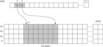
Implementation of the centre-manifold algorithm: an example of data structures to handle the multi-index sequence associated with each ordered set
 $\mathbb{M}_{m}$
for
 $m=1,\dots ,\bar{r}$
. In the considered example
 $n_{c}=3$
, with
 $\boldsymbol{m}=(m_{1},m_{2},m_{3})$
. The block of multi-indices
 $(\boldsymbol{m},p)$
associated with terms of order
 $m=|\boldsymbol{m}|+p$
is accessed in mind through the sequence of column indices given by
 $\mathtt{ordt}(m)+1,\dots ,\mathtt{ordt}(m+1)$
.

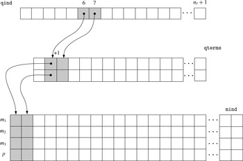
Implementation of the centre-manifold algorithm: example of data structures to handle the computation of the coefficients
 $\hat{\boldsymbol{f}}_{\boldsymbol{m},p}$
associated with a pure quadratic nonlinearity in
 $\boldsymbol{q}$
in the expression of
 $\boldsymbol{f}(\boldsymbol{q},{\it\epsilon})$
.

-
(i) Given the truncation order
$\bar{r}$
of the centre-manifold reduction, the set of integer numbers
$\mathbb{S}_{\bar{r}}\equiv [1,n_{\bar{r}}]$
is introduced to enumerate all of the terms in the truncated expansions (3.5) and (3.6). A one-to-one mapping
$s\leftrightarrow (\boldsymbol{m},p)$
is thus defined, with
$s\in \mathbb{S}_{\bar{r}}$
. In addition, for each order
$m$
the set
$\mathbb{M}_{m}=\{s_{i}\}_{i=1}^{n_{m}}$
of ordered indices corresponding to the expansion terms of degree equal to
$m$
can be introduced: (3.46)The elements of
$$\begin{eqnarray}s_{i}\leftrightarrow (\boldsymbol{m},p)\quad \text{with}~|\boldsymbol{m}|+p=m~\forall s_{i}\in \mathbb{M}_{m}.\end{eqnarray}$$
$\mathbb{M}_{m}$
are ordered at increasing power of
${\it\epsilon}$
, i.e.
$p\leqslant q$
for
$i\leqslant j~\forall s_{i},s_{j}\in \mathbb{M}_{m}$
with
$s_{i}\leftrightarrow (\boldsymbol{m},p)$
and
$s_{j}\leftrightarrow (\boldsymbol{i},q)$
. The mapping
$s\rightarrow (\boldsymbol{m},p)$
and the family of sets
$\mathbb{M}_{m}$
can be computed explicitly and stored once and for all in integer arrays. A simple example of these data structures is described in figure 1. The ordered sequences of multi-indices
$(\boldsymbol{m},p)$
associated with each set
$\mathbb{M}_{m}$
,
$m=1,\dots ,\bar{r}$
, are stored as sequential column blocks in the two-dimensional array mind of dimension
$(n_{c}+1)\times n_{\bar{r}}$
. Therefore, the
$s$
th column of mind provides the scalar entries of
$(\boldsymbol{m},p)$
for the
$s$
th term in the expansion, according to adopted enumeration of all expansion terms. In particular, in the considered example the first
$n_{c}$
rows of mind contain the elements of
$\boldsymbol{m}$
while the last row provides the value of
$p$
. For a selected order
$m=|\boldsymbol{m}|+p$
, the multi-index sequence associated with
$\mathbb{M}_{m}$
and stored in mind is accessed through the column indices given by the sequence
$\mathtt{ordt}(m)+1,\dots ,\mathtt{ordt}(m+1)$
,
$\mathtt{ordt}$
being an array of dimension
$1\times (\bar{r}+1)$
. This is illustrated in figure 1 with reference to terms of order
$m=2$
. Conversely the implementation of the inverse mapping
$(\boldsymbol{m},p)\rightarrow s$
(which is needed to compute the right-hand side
$\hat{\boldsymbol{h}}_{\boldsymbol{m},p}$
) requires a conditional loop on the elements of
$\mathbb{M}_{m=|\boldsymbol{m}|+p}$
as shown in Algorithm 2.
-
(ii) Additional data structures can be introduced to handle the computation of the coefficients
$\hat{\boldsymbol{f}}_{\boldsymbol{m},p}$
. Let us consider the case of a pure quadratic nonlinearity which is meaningful to the application to the Navier–Stokes equations. According to (3.11) we have (3.47)where summation over repeated indices is implied. Then let us introduce the indices
$$\begin{eqnarray}\{\,\hat{\boldsymbol{f}}_{\boldsymbol{m},p}\}_{i}=\mathop{\sum }_{\begin{array}{@{}c@{}}\boldsymbol{i}+\boldsymbol{n}=\boldsymbol{m}\\ q+k=p\end{array}}\unicode[STIX]{x1D60A}_{ij\ell }\{\hat{\boldsymbol{q}}_{\boldsymbol{i},q}\}_{j}\{\hat{\boldsymbol{q}}_{\boldsymbol{n},k}\}_{\ell },\quad \text{for}~i=1,\dots ,n,\end{eqnarray}$$
$s,i,j\in \mathbb{S}_{\bar{r}}$
which correspond to the involved expansion terms in the above expression: (3.48a−c )and the set
$$\begin{eqnarray}s\leftrightarrow (\boldsymbol{m},p),\quad i\leftrightarrow (\boldsymbol{i},q),\quad j\leftrightarrow (\boldsymbol{n},k),\end{eqnarray}$$
$\mathbb{D}_{s}$
of integer pairs
$(i,j)$
defined as follows: (3.49)where
$$\begin{eqnarray}\mathbb{D}_{s}:=\{(i,j),\,i,j\in \mathbb{S}_{m-1}\mid \boldsymbol{i}+\boldsymbol{n}=\boldsymbol{m}~\text{and}~q+k=p\}\end{eqnarray}$$
$|\boldsymbol{m}|>1$
is assumed. A family of sets
$\mathbb{D}_{s}$
can be derived for all
$s\in \mathbb{S}_{\bar{r}/\{\mathbb{M}_{1}\}}$
and stored once and for all in the pre-processing phase. As an example, for
$s=n_{c}+2,\dots ,n_{\bar{r}}$
, the sequence of integer pairs in
$\mathbb{D}_{s}$
can be stored as a column block in the two-dimensional array qterms of dimension
$2\times n_{s}$
, where
$n_{s}$
denotes the total number of index pairs for all of the sets
$\mathbb{D}_{s}$
. With reference to figure 2, for a selected term of the expansion labelled with
$\bar{s}$
, the corresponding integer pairs collected in
$\mathbb{D}_{\bar{s}}$
are accessed in qterms through the sequence of column indices
$\mathtt{qind}(\bar{s})+1,\dots \,,\mathtt{qind}(\bar{s}+1)$
, where qind is an array of
$1\times n_{\bar{r}}$
integers. The integer values extracted from qterms provide then access to all data structures associated with the truncated expansion, such as the multi-index data structure mind, through the introduced enumeration of all expansion terms. Once provided with these data structures, the computation of each coefficient
$\hat{\boldsymbol{f}}_{\boldsymbol{m},p}$
can be performed using a single loop on the index pairs stored in qterms, as illustrated in Algorithm 3. The definition of these data structures and of the outlined procedure can be extended to handle each term in the algebraic expression of
$\boldsymbol{f}(\boldsymbol{q},{\it\epsilon})$
.
-
(iii) When a real dynamical system is considered, both computing time and memory storage can be saved by taking directly into account the conjugate symmetry of the complex-valued terms of the expansion, i.e. those pairs of terms
$\{(\boldsymbol{m},p),(\boldsymbol{i},p)\}$
which satisfy the relation
$\boldsymbol{i}=\unicode[STIX]{x1D64B}\boldsymbol{m}$
,
$\unicode[STIX]{x1D64B}\in \mathbb{N}^{n_{c}\times n_{c}}$
being a permutation matrix defined as follows: (3.50)where
$$\begin{eqnarray}\unicode[STIX]{x1D64B}_{ij}=\left\{\begin{array}{@{}ll@{}}1\quad & \text{if}~{\it\omega}_{i}=-{\it\omega}_{j},~\text{with}~{\bf\varphi}_{i}={\bf\varphi}_{j}^{\ast }~\text{and}~{\it\omega}_{i}\neq 0\\ 0\quad & \text{otherwise},\end{array}\right.\end{eqnarray}$$
$(\cdot )^{\ast }$
is used to denote the complex conjugate. For such pairs, the expansion coefficients are related by the conjugate-symmetry conditions (3.51a,b )Hence, these coefficients can be computed and stored only once. Moreover, the elements of
$$\begin{eqnarray}\hat{\boldsymbol{q}}_{\boldsymbol{m},p}^{\ast }=\hat{\boldsymbol{q}}_{\boldsymbol{i},p},\quad \hat{\boldsymbol{g}}_{\boldsymbol{i},p}^{\ast }=\unicode[STIX]{x1D64B}\hat{\boldsymbol{g}}_{\boldsymbol{m},p}.\end{eqnarray}$$
$\hat{\boldsymbol{g}}_{\boldsymbol{m},p}$
are different from zero only if the term
$(\boldsymbol{m},p)$
is resonant.
-
(iv) The numerical solution of bordered linear systems (3.24) and (3.29), although being possible, should be avoided, especially for large-scale applications. As a matter of fact the bordered structure results in a substantial increase of the factorization fill-in when using LU solvers while for iterative solvers, a suitable preconditioner must be introduced. More conveniently, resonant solutions can be computed using the same solver employed for non-resonant systems, provided that it can handle singular linear operators. This is the case of several freely available linear-algebra packages, either based on the LU factorization or on Krylov-subspace iterations (Heroux & Willenbring Reference Heroux and Willenbring2003; Balay et al. Reference Balay, Brown, Buschelman, Gropp, Kaushik, Knepley, McInnes, Smith and Zhang2013). In particular in the algorithm provided with the UMFPACK library by Davis (Reference Davis2004) (which has been employed in our computations), during the factorization step the LU solver is able to replace the singular matrix by a fictitious invertible linear operator which is equivalent to the original matrix except for its restriction to the null space where it is substituted by the identity.














Therefore, the computation of the solution of (3.29) breaks up in a two-step regularization procedure. First, the array of the normal-form coefficients
 $\hat{\boldsymbol{g}}_{c}$
is computed by projecting the first equation in (3.29) on the
 $\ker (\unicode[STIX]{x1D647}-\imath {\it\omega}_{c}\unicode[STIX]{x1D63D})\equiv {\it\bf\Phi}_{c}$
through the adjoint eigenvectors
 ${\it\bf\Psi}_{c}$
which yields
 $$\begin{eqnarray}\hat{\boldsymbol{g}}_{c}=-{\it\bf\Psi}_{c}^{H}\hat{\boldsymbol{h}}_{\boldsymbol{m},p}.\end{eqnarray}$$
Then, the considered equation in (3.29) is recast in the form
 $$\begin{eqnarray}(\unicode[STIX]{x1D647}-\imath {\it\omega}_{c}\unicode[STIX]{x1D63D})\hat{\boldsymbol{q}}_{\boldsymbol{m},p}=\hat{\boldsymbol{h}}_{\boldsymbol{m},p}+\unicode[STIX]{x1D63D}{\it\bf\Phi}_{c}\hat{\boldsymbol{g}}_{c}=\unicode[STIX]{x1D64B}_{c}^{\bot }\hat{\boldsymbol{h}}_{\boldsymbol{m},p},\end{eqnarray}$$
where
 $\unicode[STIX]{x1D64B}_{c}^{\bot }=(\unicode[STIX]{x1D644}-\unicode[STIX]{x1D63D}{\it\bf\Phi}_{c}{\it\bf\Psi}_{c}^{H})$
is the orthogonal projector with respect to the resonant eigenmodes, thus making the above singular system well-posed. If we denote by
 $\tilde{\boldsymbol{q}}_{\boldsymbol{m},p}$
the solution issuing from the LU solver, then the solution
 $\hat{\boldsymbol{q}}_{\boldsymbol{m},p}$
of (3.29) is obtained by fixing to zero the component of
 $\tilde{\boldsymbol{q}}_{\boldsymbol{m},p}$
on the subspace spanned by the columns of
 ${\it\bf\Phi}_{c}$
, i.e.
 $\hat{\boldsymbol{q}}_{\boldsymbol{m},p}=\unicode[STIX]{x1D64B}_{c}^{\bot }\tilde{\boldsymbol{q}}_{\boldsymbol{m},p}$
.
Similarly, for Krylov solvers available within the package PETSc (Balay et al.
Reference Balay, Brown, Buschelman, Gropp, Kaushik, Knepley, McInnes, Smith and Zhang2013), a basis for the null space of the linear operator has to be provided in input to the algorithm along with the system (3.53). In this case the solution issuing from the solver already satisfies the second equation in (3.29), i.e.
 $\hat{\boldsymbol{q}}_{\boldsymbol{m},p}=\tilde{\boldsymbol{q}}_{\boldsymbol{m},p}$
, and thus the orthogonalization step is not required.
4. Application to the incompressible Navier–Stokes equations
Let us examine the application of the proposed technique to the continuous dynamical system described by the incompressible (non-dimensional) Navier–Stokes equations
 $$\begin{eqnarray}\left.\begin{array}{@{}c@{}}\displaystyle {\displaystyle \frac{\partial \boldsymbol{u}}{\partial t}}+(\boldsymbol{u}\boldsymbol{\cdot }\,\boldsymbol{{\rm\nabla}})\boldsymbol{u}+\boldsymbol{{\rm\nabla}}p-\frac{1}{\mathit{Re}}{\rm\nabla}^{2}\boldsymbol{u}=\mathbf{0},\\ \boldsymbol{{\rm\nabla}}\boldsymbol{\cdot }\,\boldsymbol{u}=0,\end{array}\right\}\end{eqnarray}$$
where
 $\boldsymbol{u}(\boldsymbol{x},t)$
denotes the velocity vector field and
 $p(\boldsymbol{x},t)$
the scalar pressure field. The fluid motion is described in a region
 ${\it\Omega}$
of the physical space where the above equations are supplemented by suitable initial and boundary conditions. In particular, these latter are assumed to be time-independent in order to deal with an autonomous dynamical system. For such a generic fluid system, the Reynolds number
 $\mathit{Re}$
defines the most obvious control parameter which is known to rule a large number of flow instabilities. Notwithstanding, different and additional control parameters can be introduced as well, appearing in the definition of the boundary conditions or being hidden in the geometrical description of
 ${\it\Omega}$
. Although the proposed centre-manifold reduction method has been introduced in § 3 within a finite-dimensional setting, it can be extended to infinite-dimensional PDE systems (Haragus & Iooss Reference Haragus and Iooss2011). Such a formalism is preferred here to avoid dealing with specific details related to the employed numerical set-up. Therefore, in the following, we will refer to continuous quantities which are intended to be replaced by their discrete counterpart when applying the procedure described in § 3. Once this parallelism has been established, the reduction to the centre manifold requires first to recast (4.1) in the general form (3.2). Let us suppose that
 $\tilde{\boldsymbol{q}}_{0}=(\boldsymbol{u}_{0}(\boldsymbol{x}),p_{0}(\boldsymbol{x}))$
is a steady-state solution of (4.1) for
 $\mathit{Re}=\mathit{Re}_{0}$
, i.e.
 $$\begin{eqnarray}\left.\begin{array}{@{}c@{}}\displaystyle (\boldsymbol{u}_{0}\boldsymbol{\cdot }\,\boldsymbol{{\rm\nabla}})\boldsymbol{u}_{0}-\frac{1}{\mathit{Re}_{0}}{\rm\nabla}^{2}\boldsymbol{u}_{0}+\boldsymbol{{\rm\nabla}}p_{0}=\mathbf{0},\\ \boldsymbol{{\rm\nabla}}\boldsymbol{\cdot }\,\boldsymbol{u}_{0}=0.\end{array}\right\}\end{eqnarray}$$
The following auxiliary variables are introduced
 $$\begin{eqnarray}\tilde{\boldsymbol{u}}(\boldsymbol{x},t)=\boldsymbol{u}(\boldsymbol{x},t)-\boldsymbol{u}_{0}(\boldsymbol{x}),\quad \tilde{p}(\boldsymbol{x},t)=p(\boldsymbol{x},t)-p_{0}(\boldsymbol{x}),\end{eqnarray}$$
which satisfy the homogeneous form of the boundary conditions imposed for
 $\boldsymbol{u}_{0}$
and
 $p_{0}$
. In addition the following definition of the control parameter
 ${\it\epsilon}$
is introduced
 $$\begin{eqnarray}{\it\epsilon}=(\mathit{Re}-\mathit{Re}_{0})/(\mathit{Re}\,\mathit{Re}_{0}).\end{eqnarray}$$
Indeed this nonlinear transformation allows the dependency on the control parameter to be exactly recast in a linear form. The alternative definition of
 ${\it\epsilon}^{2}=(\mathit{Re}-\mathit{Re}_{0})/(\mathit{Re}\,\mathit{Re}_{0})$
, which is often preferred in the multi-scale analysis (Sipp & Lebedev Reference Sipp and Lebedev2007; Meliga & Chomaz Reference Meliga and Chomaz2011), could be employed as well for
 $\mathit{Re}\geqslant \mathit{Re}_{0}$
. By inserting (4.3) and (4.4) into (4.1), this latter is rewritten as follows
 $$\begin{eqnarray}{\mathcal{B}}{\displaystyle \frac{\partial \tilde{\boldsymbol{q}}}{\partial t}}={\mathcal{L}}\tilde{\boldsymbol{q}}+{\mathcal{Q}}(\tilde{\boldsymbol{q}},{\it\epsilon}),\end{eqnarray}$$
where
 $\tilde{\boldsymbol{q}}$
is the auxiliary total flow field, i.e.
 $\tilde{\boldsymbol{q}}=(\tilde{\boldsymbol{u}},\tilde{p})^{\text{T}}$
, and the linear operators
 ${\mathcal{B}}$
and
 ${\mathcal{L}}$
are defined as
 $$\begin{eqnarray}{\mathcal{B}}\tilde{\boldsymbol{q}}=\left(\begin{array}{@{}c@{}}\tilde{\boldsymbol{u}}\\ 0\end{array}\right)\!,\quad {\mathcal{L}}\tilde{\boldsymbol{q}}=\left(\begin{array}{@{}c@{}}\displaystyle -(\boldsymbol{u}_{0}\boldsymbol{\cdot }\,\boldsymbol{{\rm\nabla}})\tilde{\boldsymbol{u}}-(\tilde{\boldsymbol{u}}\boldsymbol{\cdot }\,\boldsymbol{{\rm\nabla}})\boldsymbol{u}_{0}+\frac{1}{\mathit{Re}_{0}}{\rm\nabla}^{2}\tilde{\boldsymbol{u}}-\boldsymbol{{\rm\nabla}}\tilde{p}\\ \boldsymbol{{\rm\nabla}}\boldsymbol{\cdot }\,\tilde{\boldsymbol{u}}\end{array}\right)\!,\end{eqnarray}$$
whereas the nonlinear operator
 ${\mathcal{Q}}(\tilde{\boldsymbol{q}},{\it\epsilon})$
reads
 $$\begin{eqnarray}{\mathcal{Q}}(\tilde{\boldsymbol{q}},{\it\epsilon})=-\!\left(\begin{array}{@{}c@{}}(\tilde{\boldsymbol{u}}\boldsymbol{\cdot }\,\boldsymbol{{\rm\nabla}})\tilde{\boldsymbol{u}}+{\it\epsilon}{\rm\nabla}^{2}\boldsymbol{u}_{0}+{\it\epsilon}{\rm\nabla}^{2}\tilde{\boldsymbol{u}}\\ 0\end{array}\right)\!.\end{eqnarray}$$
According to the assumptions made in §§ 2 and 3, the system (4.5) admits the trivial equilibrium solution
 $\tilde{\boldsymbol{q}}=\mathbf{0}$
for
 ${\it\epsilon}=0$
. Its restriction to the linear terms in
 $\tilde{\boldsymbol{q}}$
clearly corresponds to the set of linearized Navier–Stokes equations describing the evolution of small perturbations around the steady base flow
 $\tilde{\boldsymbol{q}}_{0}$
. Critical eigenpairs involved in the centre-manifold reduction are thus identified as those linear global modes
 ${\bf\xi}(\boldsymbol{x},t)=\hat{{\bf\xi}}(\boldsymbol{x})\text{e}^{{\it\sigma}t}$
of the fluid system which are marginally stable, being non-trivial solutions of
 $$\begin{eqnarray}{\it\sigma}{\mathcal{B}}\hat{{\bf\xi}}={\mathcal{L}}\hat{{\bf\xi}},\end{eqnarray}$$
with the additional condition
 $\text{Re}({\it\sigma})=0$
. Critical adjoint global modes
 $\boldsymbol{{\it\eta}}(\boldsymbol{x},t)=\hat{\boldsymbol{{\it\eta}}}(\boldsymbol{x})\text{e}^{-{\it\sigma}^{\ast }t}$
need to be introduced as well:
 $$\begin{eqnarray}{\it\sigma}^{\ast }{\mathcal{B}}\hat{\boldsymbol{{\it\eta}}}={\mathcal{L}}^{\dagger }\hat{\boldsymbol{{\it\eta}}},\end{eqnarray}$$
where
 ${\mathcal{L}}^{\dagger }$
is the adjoint operator of
 ${\mathcal{L}}$
with respect to the following energy-based Hermitian scalar product
 $$\begin{eqnarray}\langle \tilde{\boldsymbol{q}}_{A},\tilde{\boldsymbol{q}}_{B}\rangle =\int _{{\it\Omega}}\tilde{\boldsymbol{q}}_{A}^{\ast }\boldsymbol{\cdot }\,\tilde{\boldsymbol{q}}_{B}\text{d}{\it\Omega}.\end{eqnarray}$$
The direct and adjoint global modes are normalized such that
 $\langle \hat{\boldsymbol{{\it\eta}}}_{A},{\mathcal{B}}\hat{{\bf\xi}}_{A}\rangle =1$
. For further details on the global mode analysis and on their computation see the recent reviews by Theofilis (Reference Theofilis2011) and Luchini & Bottaro (Reference Luchini and Bottaro2014).
4.1. Numerical methods
In the following sections we describe the application of the centre-manifold reduction to two different flow configurations, namely the flow past an isolated cylinder and the flow past two cylinders arranged side-by-side with respect to the free stream. In both cases the Navier–Stokes equations are made dimensionless using the cylinder diameter
 $D^{\ast }$
, the velocity of the free stream
 $U_{\infty }^{\ast }$
, and the (constant) density
 ${\it\rho}^{\ast }$
, the Reynolds number being defined as
 $\mathit{Re}=U_{\infty }^{\ast }D^{\ast }/{\it\nu}^{\ast }$
, where
 ${\it\nu}^{\ast }$
denotes the kinematic viscosity. The Navier–Stokes equations have been spatially discretized in conservative form on a rectangular computational domain
 ${\it\Omega}_{c}$
. A standard second-order finite-difference scheme is used on a Cartesian, smoothly varying staggered grid and the no-slip boundary conditions on the solid surfaces are imposed using an immersed-boundary method which preserves the second-order accuracy of the discretization (see Giannetti & Luchini Reference Giannetti and Luchini2007, for further details).
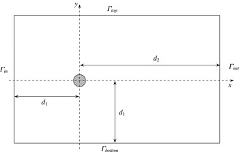
With reference to figure 3, a Cartesian coordinate system is adopted with its origin being located on the cylinder centre and its
 $x$
-axis being aligned with the uniform free-stream velocity. In such a reference system the velocity vector field is described by means of its components
 $\boldsymbol{u}=(u,v)$
. In our computational set-up, the solid body is placed at a distance
 $d_{1}=50$
from the inlet
 ${\it\Gamma}_{in}$
and the upper and lower boundary,
 ${\it\Gamma}_{top}$
and
 ${\it\Gamma}_{bottom}$
, while the outlet
 ${\it\Gamma}_{out}$
is located at a distance
 $d_{2}=150$
from the origin. On
 ${\it\Gamma}_{out}$
, (4.1) are supplemented with the boundary conditions
 $-p+2\mathit{Re}^{-1}\partial u/\partial x=0$
and
 $\partial v/\partial x=0$
. On
 ${\it\Gamma}_{in}$
,
 ${\it\Gamma}_{top}$
and
 ${\it\Gamma}_{bottom}$
, the vorticity is set to zero as well as the velocity component
 $v$
. The computational domain is discretized using
 $600\times 300$
grid points with a clustering near the cylinder surface. More precisely, a uniform mesh is adopted in the small square subdomain
 $[-1,1]\times [1,1]$
enclosing the body, with the finest mesh size being
 ${\rm\Delta}x={\rm\Delta}y=0.02$
.
Sketch of the computational domain
 ${\it\Omega}_{c}$
employed for numerical investigations of the flow past an isolated cylinder.

For the numerical simulation of the flow past the two side-by-side cylinders, the same domain size and boundary conditions are employed except on the boundaries
 ${\it\Gamma}_{in}$
,
 ${\it\Gamma}_{top}$
and
 ${\it\Gamma}_{bottom}$
where the vorticity is set to zero and the flow perturbation produced by the two cylinders on the incoming uniform stream is assumed to decay to zero as the leading term of the potential flow around it. The two cylinder centres are aligned on the
 $y$
-axis and symmetrically positioned with respect to the
 $x$
-axis. In this case, the uniform subgrid is extended to the subdomain
 $[-1,1]\times [-2.5,2.5]$
and a total of
 $600\times 450$
grid points are employed. For further details see also Carini, Giannetti & Auteri (Reference Carini, Giannetti and Auteri2014a
,Reference Carini, Giannetti and Auteri
b
).
In order to compute the centre-manifold approximation, both the base flow and the related critical global modes are required. For each considered configuration, the basic flow state is obtained by solving the steady version of (4.1) by Newton iterations. Direct and adjoint global modes are then computed using the Krylov–Arnoldi algorithm implemented in the ARPACK library (Lehoucq, Sorensen & Yang Reference Lehoucq, Sorensen and Yang1998) based upon a shift-invert strategy. More precisely, a discrete adjoint approach is adopted. In this way the proper boundary conditions for the adjoint problem are accounted for automatically and the biorthogonality condition between direct and adjoint eigenfunctions is satisfied up to machine precision in the discrete setting.
Direct numerical simulations (DNS) are performed by advancing in time the spatially discretized nonlinear equations using the hybrid third-order Runge–Kutta/Crank–Nicolson scheme of Rai & Moin (Reference Rai and Moin1991). The same scheme is also employed for time integration of the amplitude equations (3.6) obtained from the centre-manifold reduction. All of the required matrix inversions are handled by means of the sparse LU solver provided with the software package UMFPACK (Davis Reference Davis2004).
4.2. Flow past a circular cylinder
The two-dimensional flow past a circular cylinder has been extensively investigated both experimentally and numerically owing to its practical and theoretical relevance (Williamson Reference Williamson1996). For such flow, the primary instability occurs via a Hopf bifurcation of the basic steady state at
 $\mathit{Re}\approx 47$
, leading to the onset of an alternate vortex shedding with the formation of the so-called Bernard–von Kármán vortex street. In the context of hydrodynamic stability, the bifurcating cylinder flow dynamics is usually described by means of the Stuart–Landau equation:
 $$\begin{eqnarray}{\displaystyle \frac{\text{d}A}{\text{d}{\it\tau}}}={\it\lambda}A-{\it\mu}A|A|^{2},\end{eqnarray}$$
where
 $A({\it\tau})$
denotes the renormalized critical mode amplitude,
 ${\it\tau}={\it\epsilon}\,t$
represents the ‘slow’ time scale of its nonlinear evolution and
 ${\it\lambda},{\it\mu}\in \mathbb{C}$
are the so-called Landau constants. The values of
 ${\it\lambda}$
and
 ${\it\mu}$
have been computed by Sipp & Lebedev (Reference Sipp and Lebedev2007) and Meliga & Chomaz (Reference Meliga and Chomaz2011) while performing a weakly nonlinear global analysis of this flow using the classical multiple-scale approach.
In order to validate our technique, the centre-manifold reduction is applied to the considered flow and obtained results are then compared with those described in the previously cited works. By performing a linear stability analysis, critical values of the Reynolds number and of the global mode frequency
 $\mathit{St}_{0}=\text{Im}({\it\sigma})/2{\rm\pi}$
are found,
 $\mathit{Re}_{0}\sim 46.51$
and
 $\mathit{St}_{0}\sim 0.117$
, respectively, which are in good agreement with those computed by Giannetti & Luchini (Reference Giannetti and Luchini2007), Sipp & Lebedev (Reference Sipp and Lebedev2007), Marquet, Sipp & Jacquin (Reference Marquet, Sipp and Jacquin2008) and Meliga & Chomaz (Reference Meliga and Chomaz2011). Since the Hopf bifurcation involves a conjugate pair of critical eigenvalues, only a single amplitude equation will be considered in the following as done in § 3.2. At order
 $\bar{r}=4$
we obtain
 $$\begin{eqnarray}{\dot{a}}=\tilde{g}_{1}({\it\epsilon})a+\tilde{g}_{2}({\it\epsilon})a|a|^{2},\end{eqnarray}$$
where
 $$\begin{eqnarray}\left.\begin{array}{@{}l@{}}\tilde{g}_{1}({\it\epsilon})={\hat{g}}_{(1,0),0}+{\hat{g}}_{(1,0),1}{\it\epsilon}+{\hat{g}}_{(1,0),2}{\it\epsilon}^{2}+{\hat{g}}_{(1,0),3}{\it\epsilon}^{3},\\ \tilde{g}_{2}({\it\epsilon})={\hat{g}}_{(2,1),0}+{\hat{g}}_{(2,1),1}{\it\epsilon}.\end{array}\!\right\}\end{eqnarray}$$
The third-order form of the amplitude equation is simply derived by dropping the terms
 ${\hat{g}}_{(1,0),3}{\it\epsilon}^{3}$
and
 ${\hat{g}}_{(2,1),1}{\it\epsilon}$
in the above expressions. The computed values of the normal-form coefficients are listed in table 2. The identification of the Landau constants follows from the relation between
 $a(t)$
and
 $A({\it\tau})$
with
 $$\begin{eqnarray}a(t)=\sqrt{{\it\epsilon}}A({\it\epsilon}t)\exp (\text{i}{\it\omega}_{0}t).\end{eqnarray}$$
Therefore,
 ${\it\lambda}={\hat{g}}_{(1,0),1}$
and
 ${\it\mu}=-{\hat{g}}_{(2,1),0}$
. Both
 ${\it\lambda}$
and the ratio
 $\text{Im}({\it\mu})/\text{Re}({\it\mu})$
are intrinsic quantities, i.e. they do not depend on the adopted global mode normalization since their appear in the expression of the limit-cycle frequency derived from the normal-form analysis, as shown by Sipp & Lebedev (Reference Sipp and Lebedev2007). A comparison with the values computed by these latter authors and by Meliga & Chomaz (Reference Meliga and Chomaz2011) is reported in table 3: good agreement is observed with a small deviation affecting the value of
 $\text{Im}({\it\mu})/\text{Re}({\it\mu})$
. In their work Sipp & Lebedev (Reference Sipp and Lebedev2007) have shown that the computation of
 ${\it\mu}$
is very sensitive to the downstream location of the outlet boundary and in order to get converged results this boundary must be moved at least 50 diameters downstream of the cylinder position. This requirement is fulfilled by our computational domain and, hence, the small discrepancy in the value of
 $\text{Im}({\it\mu})/\text{Re}({\it\mu})$
may be ascribed to the different numerical discretization.
Centre-manifold reduction of the first Hopf bifurcation of the cylinder wake: computed normal-form coefficients up to order
 $\bar{r}=4$
.

Landau constants
 ${\it\lambda}$
,
 ${\it\mu}$
of the first Hopf bifurcation of the cylinder wake: comparison of computed values with those reported by other authors.

Some of the computed nonlinear global modes
 $\hat{\boldsymbol{u}}_{\boldsymbol{m},p}$
are illustrated in figure 4. These modes exactly correspond to those reported by Sipp & Lebedev (Reference Sipp and Lebedev2007) and Meliga & Chomaz (Reference Meliga and Chomaz2011) except for a scale factor which is due to a different choice in the normalization of the critical eigenmodes. Consistently with their physical interpretation the same spatial pattern is reproduced: as an example the mode
 $\hat{\boldsymbol{u}}_{(0,0),1}$
, figure 4(a), provides the base-flow correction due to an
 ${\it\epsilon}$
increment of
 $\mathit{Re}^{-1}$
while the modes
 $\hat{\boldsymbol{u}}_{(1,1),0}$
, figure 4(b), and
 $\hat{\boldsymbol{u}}_{(2,0),0}$
, figure 4(c), represent the second-order mean-flow correction and the second-harmonic interaction, respectively. In addition, figure 4(d) shows the mode associated with the resonant term
 $a{\it\epsilon}$
, i.e.
 $\hat{\boldsymbol{u}}_{(1,0),1}$
.
Nonlinear modes appearing in the centre-manifold reduction of the first Hopf bifurcation of the single cylinder wake, streamwise velocity component (real part): (a)
 $\hat{u} _{(0,0),1}$
; (b)
 $\hat{u} _{(1,1),0}$
; (c)
 $\hat{u} _{(2,0),0}$
; (d)
 $\hat{u} _{(1,0),1}$
.

Unsteady flow past a single circular cylinder at
 $\mathit{Re}=48~({\it\epsilon}=6.7\times 10^{-4})$
: comparison of the aerodynamic coefficients and the Strouhal number obtained from DNS with those computed from the centre-manifold reduction of the Hopf bifurcation at
 $\bar{r}=3$
and
 $\bar{r}=4$
. Here
 $\bar{C}_{D}$
denotes the mean drag coefficient while
 $C_{L}^{\prime }$
and
 $C_{D}^{\prime }$
indicate the maximum amplitude of the lift- and drag-coefficient fluctuations, respectively.

In the neighbourhood of
 $\mathit{Re}_{0}$
, the computed centre-manifold approximation provides us with a reduced-order model of the unsteady cylinder wake. For
 $\mathit{Re}=48~({\it\epsilon}=6.7\times 10^{-4})$
, the non-dimensional shedding frequency
 $St$
associated with the asymptotic limit-cycle solution of (4.12) is reported in table 4 for
 $\bar{r}=3$
and
 $\bar{r}=4$
. As expected, these values match very well that computed from the DNS which is also indicated. Once the asymptotic limit-cycle solution of (4.12) has been derived, the approximation of the whole flow field at each time instant is straightforwardly computed by exploiting (3.5). A comparison of the predicted values of the aerodynamic coefficients with those obtained from DNS is also reported in table 4. The phase diagrams of both the aerodynamic coefficients and the velocity fluctuations sampled at three distinct points in the flow field are reported in figures 5 and 6, respectively. These results indicate that a good approximation of the fully developed cylinder vortex shedding is obtained for
 $\bar{r}=4$
. In figure 7(a–c) the streamlines of the centre-manifold-reconstructed flow field are compared with those of the DNS snapshot computed at the same shedding phase: the same streamfunction contour levels are employed in both cases, thus highlighting that vortical structures in the near-wake region are well captured by means of the nonlinear global mode superposition in (3.5). In contrast, in the far-wake region, spurious eddies affect the reconstructed flow field as shown in figure 7(b–d). Such results suggest that while the centre-manifold description is able to correctly reproduce the flow behaviour where the self-sustained global instability develops, i.e. in the so-called wavemaker region (Giannetti & Luchini Reference Giannetti and Luchini2007), it fails to adequately capture the flow dynamics in the far-wake region where nonlinear interactions of damped linear modes can still play an important role.
Flow past a single cylinder at
 $\mathit{Re}=48$
: phase-portrait of the aerodynamic coefficients over a time interval of 300 non-dimensional time units. Comparison between DNS (black lines) and centre-manifold approximation of the flow at order
 $\bar{r}=3$
(dark grey lines) and
 $\bar{r}=4$
(light grey lines).

Flow past a single cylinder at
 $\mathit{Re}=48$
: phase portrait of the velocity field sampled at (a)
 $(x_{s},y_{s})=(1.5,0)$
, (b)
 $(x_{s},y_{s})=(1.5,1.5)$
and (c)
 $(x_{s},y_{s})=(1.5,-1.5)$
. Comparison between DNS (black lines) and centre-manifold approximation of the flow at order
 $\bar{r}=3$
(dark grey lines) and
 $\bar{r}=4$
(light grey lines).

Flow past a single cylinder at
 $\mathit{Re}=48$
: streamlines and vorticity fields computed at the same shedding phase indicated in figure 5 (grey–black dots). Comparison between DNS (a)–(b) and centre-manifold approximation at order
 $\bar{r}=4$
(c)–(d). The same contour levels are employed in (a) and (c) for the streamline representation.

4.2.1. Amplitude power-series convergence
A critical comparison of the obtained results with DNS data should take into account the issue of convergence of the power series in the critical amplitudes while varying the bifurcation parameter
 ${\it\epsilon}$
. The asymptotic behaviour of this power series and the estimation of its radius of convergence can be investigated by exploiting the capability to easily compute high-order amplitude equations provided by the proposed method. For this purpose let us consider the general expression of the amplitude equation associated with the Hopf bifurcation
 $$\begin{eqnarray}{\dot{a}}=\tilde{g}_{1}({\it\epsilon})a+\mathop{\sum }_{k=2}^{\infty }\tilde{g}_{k}({\it\epsilon})a|a|^{2(k-1)},\end{eqnarray}$$
where in our approach the dependence of the normal-form coefficients on the bifurcation parameter is also approximated in power series of the parameter itself, as shown in (4.13) for third- and fourth-order centre-manifold approximations. For a given value of the bifurcation parameter
 ${\it\epsilon}=\bar{{\it\epsilon}}$
,
 $\text{d}|a|/\text{d}t\rightarrow 0$
as
 $t\rightarrow \infty$
if an asymptotic limit cycle solution exists for this solution. By denoting with
 ${\it\varrho}_{\infty }$
the asymptotic value approached by
 $|a|$
,
 ${\it\varrho}_{\infty }$
can be computed as a root of the real-valued coefficient polynomial
 $$\begin{eqnarray}\text{Re}(\tilde{g}_{1}({\it\epsilon})){\it\varrho}_{\infty }+\mathop{\sum }_{k=2}^{\infty }\text{Re}(\tilde{g}_{k}({\it\epsilon})){\it\varrho}_{\infty }^{2{\it\kappa}-1}=0.\end{eqnarray}$$
Once the value of
 ${\it\varrho}_{\infty }$
has been obtained, the limit-cycle circular frequency
 ${\it\omega}_{\infty }$
is given by
 $$\begin{eqnarray}{\it\omega}_{\infty }=\text{Im}(\tilde{g}_{1}({\it\epsilon}))+\mathop{\sum }_{k=2}^{\infty }\text{Im}(\tilde{g}_{k}({\it\epsilon})){\it\varrho}_{\infty }^{2({\it\kappa}-1)}.\end{eqnarray}$$
At this point in order to estimate the range of values of
 ${\it\epsilon}$
for which the amplitude power series converges, the expansions (3.5) and (3.6) are truncated at increasing order
 $\bar{r}$
of the centre-manifold approximation, and for each considered value of
 ${\it\epsilon}$
and
 $\bar{r}$
,
 ${\it\varrho}_{\infty }$
is obtained by computing the roots of the truncated form of (4.16). Obviously only real positive roots make sense and when multiple, real, strictly positive solutions are found, only the one which can be ‘continued’ from the third-order normal form is considered. The present analysis has been applied to the cylinder wake by computing the centre-manifold reduction of the related Hopf bifurcation up to
 $\bar{r}=10$
. The obtained values of
 ${\it\varrho}_{\infty }$
are reported in figure 8 indicating that the convergence radius of the series in terms of
 ${\it\epsilon}$
,
 ${\it\epsilon}_{c}$
is rather small, with
 ${\it\epsilon}_{c}\approx 10^{-4}$
(
 $\mathit{Re}\approx 46.73$
compared with
 $\mathit{Re}_{0}=46.51$
). Corresponding values of
 $\mathit{St}_{\infty }=2{\rm\pi}/{\it\omega}_{\infty }$
are also reported in table 5. Therefore, the computed centre-manifold approximation for
 $\mathit{Re}=48$
falls outside the radius of convergence of the series, a fact which could also explain the unphysical flow-field reconstruction in the far-wake region.
Centre-manifold reduction of the first Hopf bifurcation of the cylinder wake: computed values of the limit cycle amplitude
 ${\it\varrho}_{\infty }$
for different values of
 ${\it\epsilon}$
and of the truncation order
 $\bar{r}$
of the expansion series up to
 $\bar{r}=10$
. For
 ${\it\epsilon}=5\times 10^{-4}$
and
 $\bar{r}=9$
the limit cycle solution does not exist.

Centre-manifold reduction of the first Hopf bifurcation of the cylinder wake: computed values of the universal limit-cycle frequency
 $\mathit{St}_{\infty }=2{\rm\pi}/{\it\omega}_{\infty }$
for different values of
 ${\it\epsilon}$
and of the truncation order
 $\bar{r}$
of the expansion series up to
 $\bar{r}=10$
. Note that for
 ${\it\epsilon}=5\times 10^{-4}$
and
 $\bar{r}=9$
the limit cycle solution does not exist.

4.3. Flow past two side-by-side circular cylinders
Despite the simple geometry, it is known that the flow past two circular cylinders in side-by-side arrangement is characterized by the onset of various flow instabilities, depending on the Reynolds number and even more on the gap spacing between the two cylinder surfaces
 $g=g^{\ast }/D^{\ast }$
. A global stability analysis of this flow has been performed by Akinaga & Mizushima (Reference Akinaga and Mizushima2005), Mizushima & Ino (Reference Mizushima and Ino2008) and more recently by Carini et al. (Reference Carini, Giannetti and Auteri2014a
), showing that for different values of
 $g$
and
 $\mathit{Re}$
, the steady symmetric base flow becomes linearly unstable due to different global modes either associated with the onset of vortex shedding or with the occurrence of a steady asymmetric flow characterized by the deflection of the fluid stream through the gap. In particular, three codimension-two points have been found in the related bifurcation diagram.
As a more demanding application of the proposed method, we compute the centre-manifold approximation of the considered flow in the codimension-two pitchfork-Hopf bifurcation point which is associated with the simultaneous criticality of the steady antisymmetric (AS) mode and of the oscillatory (IP) mode of in-phase, synchronized vortex shedding. According to the neutral curves reported in Carini et al. (Reference Carini, Giannetti and Auteri2014a
) this point is located at
 $(g_{0},\mathit{Re}_{0})=(0.725,56.46)$
. For these values of the parameters, the computed critical eigenvalues corresponding to the AS and the IP modes are
 ${\it\sigma}_{1}=-2.1145\times 10^{-10}+6.4185\times 10^{-17}\text{i}$
and
 ${\it\sigma}_{2,3}=-4.8497\times 10^{-10}\pm 0.6618\text{i}$
, respectively. These modes are depicted in figure 9(a,b) by means of the
 $u$
component of the velocity field (real part). In this case two bifurcation parameters are present, namely
 ${\it\epsilon}_{1}=(\mathit{Re}-\mathit{Re}_{0})/(\mathit{Re}\mathit{Re}_{0})$
and
 ${\it\epsilon}_{2}=g-g_{0}$
. Although the proposed technique can be extended to deal with an arbitrary number of parameters, in the present work only one of two bifurcation parameters is considered at a time while the other is fixed to its critical value. Thus, the centre-manifold reduction is repeated twice, once for
 ${\it\epsilon}={\it\epsilon}_{1}$
and then for
 ${\it\epsilon}={\it\epsilon}_{2}$
. However, the parameter
 $g$
does not appear explicitly in the governing equations (4.1), neither in the expression of the boundary conditions. For such a case where the dependency on the bifurcation parameter is hidden in the domain definition or, more generally, in the mathematical formulation of the governing equations, we can resort to its Taylor-series approximation. This can be done by expanding
 $\boldsymbol{F}(\cdot ,{\it\epsilon})$
in the neighbourhood of
 ${\it\epsilon}=0$
 $$\begin{eqnarray}\boldsymbol{F}(\cdot ,{\it\epsilon})\approx \boldsymbol{F}_{0}(\cdot )+{\it\epsilon}\boldsymbol{F}_{{\it\epsilon}}(\cdot )+{\it\epsilon}^{2}\boldsymbol{F}_{{\it\epsilon}^{2}}(\cdot )+\cdots\end{eqnarray}$$
where the nonlinear operators
 $\boldsymbol{F}_{{\it\epsilon}^{k}}(\cdot )$
are formally defined as follows
 $$\begin{eqnarray}\boldsymbol{F}_{{\it\epsilon}^{k}}(\cdot )=\left.\frac{1}{k!}\frac{\text{d}^{k}\boldsymbol{F}(\cdot ,{\it\epsilon})}{\text{d}{\it\epsilon}^{k}}\right|_{{\it\epsilon}=0},\end{eqnarray}$$
and their action can be numerically computed by means of suitable finite-difference formulas. As an example
 $$\begin{eqnarray}\left.\frac{\text{d}\boldsymbol{F}(\boldsymbol{q},{\it\epsilon})}{\text{d}{\it\epsilon}}\right|_{{\it\epsilon}=0}\approx \frac{\boldsymbol{F}(\boldsymbol{q},{\rm\Delta}{\it\epsilon})-\boldsymbol{F}(\boldsymbol{q},0)}{{\rm\Delta}{\it\epsilon}},\end{eqnarray}$$
with
 ${\rm\Delta}{\it\epsilon}$
being a positive and small-enough
 ${\it\epsilon}$
increment. This has been done in the present computations by exploiting our implementation of the immersed-boundary technique, with the body surface being described analytically.
Nonlinear modes appearing in the centre-manifold reduction of the pitchfork-Hopf bifurcation at
 $(g_{0},\mathit{Re}_{0})=(0.725,56.46)$
in the flow past two side-by-side cylinders: streamwise velocity component (real part): (a)
 $\hat{u} _{(1,0,0),0}$
(AS mode); (b)
 $\hat{u} _{(0,1,0),0}$
(IP mode); (c)
 $\hat{u} _{(0,0,0),1}^{{\it\epsilon}_{1}}$
; (d)
 $\hat{u} _{(0,0,0),1}^{{\it\epsilon}_{2}}$
; (e)
 $\hat{u} _{(2,0,0),0}$
; (f)
 $\hat{u} _{(1,1,0),0}$
; (g)
 $\hat{u} _{(3,0,0),0}$
; (h)
 $\hat{u} _{(1,2,0),0}$
.

Centre-manifold reduction of the incompressible Navier–Stokes system at the codimension-two bifurcation point in the flow past two side-by-side cylinders: computed coefficients of the pitchfork-branch of the third-order normal form (4.21) (first equation) for both
 ${\it\epsilon}={\it\epsilon}_{1}$
and
 ${\it\epsilon}={\it\epsilon}_{2}$
.

Centre-manifold reduction of the incompressible Navier–Stokes system at the codimension-two bifurcation point in the flow past two side-by-side cylinders: computed coefficients of the Hopf branch of the third-order normal form (4.21) (second equation) for both
 ${\it\epsilon}={\it\epsilon}_{1}$
and
 ${\it\epsilon}={\it\epsilon}_{2}$
.

For the considered bifurcation, equation (3.4) can be reduced to a system of one real-valued and one complex-valued equations since only one of the two amplitude equations associated with the pair
 ${\it\sigma}_{2,3}$
is considered. Let us denote with
 $a_{1}(t)$
the real critical amplitude associated with the pitchfork branch and with
 $a_{2}(t)$
the complex one related to the Hopf branch. Then the computed normal form at
 $\bar{r}=3$
reads
 $$\begin{eqnarray}\left.\begin{array}{@{}l@{}}\displaystyle {\dot{a}}_{1}=\tilde{g}_{1,1}({\it\epsilon})+\tilde{g}_{1,2}({\it\epsilon})a_{1}+\tilde{g}_{1,3}({\it\epsilon})a_{1}^{2}+\tilde{g}_{1,4}({\it\epsilon})|a_{2}|^{2}+\tilde{g}_{1,5}({\it\epsilon})|a_{2}|^{2}a_{1}+\tilde{g}_{1,6}({\it\epsilon})a_{1}^{3},\\ \displaystyle {\dot{a}}_{2}=\tilde{g}_{2,1}({\it\epsilon})a_{2}+\tilde{g}_{2,2}({\it\epsilon})a_{1}a_{2}+\tilde{g}_{2,3}({\it\epsilon})a_{1}^{2}a_{2}+\tilde{g}_{2,4}({\it\epsilon})a_{2}|a_{2}|^{2},\end{array}\right\}\end{eqnarray}$$
where
 $$\begin{eqnarray}\left.\begin{array}{@{}l@{}}\tilde{g}_{1,1}({\it\epsilon})={\hat{g}}_{(0,0,0),1}{\it\epsilon}+{\hat{g}}_{(0,0,0),2}{\it\epsilon}^{2}+{\hat{g}}_{(0,0,0),3}{\it\epsilon}^{3},\\ \tilde{g}_{1,2}({\it\epsilon})={\hat{g}}_{(1,0,0),1}{\it\epsilon}+{\hat{g}}_{(1,0,0),2}{\it\epsilon}^{2},\\ \tilde{g}_{1,3}({\it\epsilon})={\hat{g}}_{(2,0,0),0}+{\hat{g}}_{(2,0,0),1}{\it\epsilon},\\ \tilde{g}_{1,4}({\it\epsilon})={\hat{g}}_{(0,1,1),0}+{\hat{g}}_{(0,1,1),1}{\it\epsilon},\\ \tilde{g}_{1,5}({\it\epsilon})={\hat{g}}_{(1,1,1),0},\\ \tilde{g}_{1,6}({\it\epsilon})={\hat{g}}_{(3,0,0),0},\end{array}\right\}\end{eqnarray}$$
and
 $$\begin{eqnarray}\left.\begin{array}{@{}l@{}}\tilde{g}_{2,1}({\it\epsilon})={\hat{g}}_{(0,1,0),0}+{\hat{g}}_{(0,1,0),1}{\it\epsilon}+{\hat{g}}_{(0,1,0),2}{\it\epsilon}^{2},\\ \tilde{g}_{2,2}({\it\epsilon})={\hat{g}}_{(1,1,0),0}+{\hat{g}}_{(1,1,0),1}{\it\epsilon},\\ \tilde{g}_{2,3}({\it\epsilon})={\hat{g}}_{(2,1,0),0},\\ \tilde{g}_{2,4}({\it\epsilon})={\hat{g}}_{(0,2,1),0}.\end{array}\right\}\end{eqnarray}$$
The computed values of these coefficients for
 ${\it\epsilon}={\it\epsilon}_{1}$
and
 ${\it\epsilon}={\it\epsilon}_{2}$
are listed in tables 6 and 7. Some of the computed nonlinear global modes are illustrated in figure 9 by means of the
 $u$
component of the inherent velocity field. The first-order base flow correction, i.e. the mode
 $\hat{\boldsymbol{u}}_{(0,0,0),1}$
, is shown in figure 9(c,d) for
 ${\it\epsilon}={\it\epsilon}_{1}$
and
 ${\it\epsilon}={\it\epsilon}_{2}$
, respectively. In particular, the correction induced by a reduction of the gap size, i.e. a negative
 ${\it\epsilon}_{2}$
variation, results in a reduction of the velocity through the gap, which is consistent with the results reported by Mizushima & Ino (Reference Mizushima and Ino2008). The remaining nonlinear modes in figure 9 are associated with other terms such as the second-order coupling term
 $a_{1}a_{2}$
illustrated in figure 9(f) and the third-order terms
 $a_{1}^{3}$
and
 $a_{1}a_{2}^{2}$
illustrated in figures 9(g) and 9(h), respectively. All of these modes do not depend on the choice of the bifurcation parameter.
It is worthwhile to note that the proposed algorithm can provide directly the normal form unfolded with respect to those symmetries that are not explicitly enforced in the dynamical system model. With respect to the case where the symmetry condition is exactly satisfied, additional normal-form coefficients are found slightly different from zero. This can be shown by examining the pure pitchfork branch of the considered codimension-two bifurcation. Setting
 $a_{2}=0$
in the first equation of (4.21) we obtain
 $$\begin{eqnarray}{\dot{a}}_{1}=\tilde{g}_{1,1}({\it\epsilon})+\tilde{g}_{1,2}({\it\epsilon})a_{1}+\tilde{g}_{1,3}({\it\epsilon})a_{1}^{2}+\tilde{g}_{1,6}({\it\epsilon})a_{1}^{3}.\end{eqnarray}$$
The above normal form indicates that the pitchfork branch is imperfect. Indeed the inherent symmetry with respect to the
 $x$
-axis is not enforced at the discrete level and small numerical errors are responsible for the coefficients
 $\tilde{g}_{1,1}({\it\epsilon})$
and
 $\tilde{g}_{1,3}({\it\epsilon})$
being different from zero. However, in the neighbourhood of the bifurcation point with
 $|{\it\epsilon}|\ll 1$
, these terms are negligible compared with the other terms of (4.24) and they can be discarded, thus recovering the normal form of the generic pitchfork. Asymptotically (4.24) reduces to a third-order polynomial equation in the unknown
 $a_{1}$
: the three related roots
 $\bar{a}_{1,0}$
,
 $\bar{a}_{1,-}$
and
 $\bar{a}_{1,+}$
can be interpreted as perturbed solutions of the generic normal form due to the small deviation from the exact symmetric condition. Indeed for
 ${\it\epsilon}_{2}=0.005$
, (
 $g=0.72$
), we obtain
 $\bar{a}_{1,0}=1.161\times 10^{-4}$
,
 $\bar{a}_{1,-}=-0.2164$
and
 $\bar{a}_{1,+}=0.2166$
to be compared with the values
 $\bar{a}_{1,0}=0$
and
 $\bar{a}_{1,\pm }=\pm 0.2165$
computed using the generic normal form. The unfolded solution
 $\bar{a}_{1,+}$
can be used to approximate the steady asymmetric flow arising through the pitchfork bifurcation. In figure 10 the centre-manifold reconstructed flow field at
 $\bar{r}=3$
is compared with the asymmetric steady solution of (4.1) computed by means of Newton iterations for
 $\mathit{Re}=\mathit{Re}_{0}$
and
 $g=0.72$
. The same stream-function levels are employed in figure 10(a,b). Both the small gap-flow deflection and the recirculating flow structures behind the two cylinders are accurately captured and a very good agreement is obtained in terms of the aerodynamic coefficients which are listed in table 8.
Streamlines of the steady asymmetric flow past two side-by-side circular cylinders for
 $g=0.72$
and
 $\mathit{Re}=\mathit{Re}_{0}$
: comparison between DNS (a) and centre-manifold approximation (b) at
 $\bar{r}=3$
. The same contour levels are employed in both figures.

Steady asymmetrical flow for
 $\mathit{Re}=\mathit{Re}_{0}$
and
 $g=0.72$
: aerodynamic force coefficients of the two cylinders. Comparison between the solution of the steady Navier–Stokes equations (DNS) and its centre-manifold approximation.

4.3.1. Codimension-two normal-form analysis
The obtained results can be used to investigate the phase–space portrait of the considered flow in the neighbourhood of its codimension-two bifurcation point. Based on classical bifurcation theory (Kuznetsov Reference Kuznetsov1998), the following third-order normal form is derived from (4.21):
 $$\begin{eqnarray}\left.\begin{array}{@{}l@{}}\displaystyle {\dot{b}}=b({\it\lambda}_{1}({\it\epsilon}_{1},{\it\epsilon}_{2})+{\it\gamma}_{11}b^{2}+{\it\gamma}_{12}r^{2}),\\ \displaystyle {\dot{r}}=r({\it\lambda}_{2}({\it\epsilon}_{1},{\it\epsilon}_{2})+{\it\gamma}_{21}b^{2}+{\it\gamma}_{22}r^{2}),\\ \displaystyle \dot{{\it\phi}}={\it\omega}({\it\epsilon}_{1},{\it\epsilon}_{2}),\end{array}\right\}\end{eqnarray}$$
where
 $b=|a_{1}|$
and the polar-coordinate transformation
 $a_{2}(t)=r(t)\text{e}^{\text{i}{\it\phi}(t)}$
has been introduced. In the derivation of the above equations, the generic form of the pitchfork bifurcation is assumed, thus making possible to replace
 $a_{1}$
by its modulus. The coefficients
 ${\it\gamma}_{ij}$
are simply given by
 ${\it\gamma}_{11}={\hat{g}}_{(3,0,0),0}$
,
 ${\it\gamma}_{12}={\hat{g}}_{(1,1,1),0}$
,
 ${\it\gamma}_{21}=\text{Re}\{{\hat{g}}_{(2,1,0),0}\}$
and
 ${\it\gamma}_{22}=\text{Re}\{{\hat{g}}_{(0,2,1),0}\}$
. Their values do not depend on the definition of
 ${\it\epsilon}$
. In contrast, the remaining coefficients in (4.25) are assumed to depend linearly on both bifurcation parameters:
 $$\begin{eqnarray}\left.\begin{array}{@{}l@{}}{\it\lambda}_{1}({\it\epsilon}_{1},{\it\epsilon}_{2})={\hat{g}}_{(1,0,0),1}^{({\it\epsilon}_{1})}{\it\epsilon}_{1}+{\hat{g}}_{(1,0,0),1}^{({\it\epsilon}_{2})}{\it\epsilon}_{2},\\ {\it\lambda}_{2}({\it\epsilon}_{1},{\it\epsilon}_{2})=\text{Re}\{{\hat{g}}_{(0,1,0),1}^{({\it\epsilon}_{1})}\}{\it\epsilon}_{1}+\text{Re}\{{\hat{g}}_{(0,1,0),1}^{({\it\epsilon}_{2})}\}{\it\epsilon}_{2},\\ {\it\omega}({\it\epsilon}_{1},{\it\epsilon}_{2})=\text{Im}\{{\hat{g}}_{(0,1,0),0}\}+\text{Im}\{{\hat{g}}_{(0,1,0),1}^{({\it\epsilon}_{1})}\}{\it\epsilon}_{1}+\text{Im}\{{\hat{g}}_{(0,1,0),1}^{({\it\epsilon}_{2})}\}{\it\epsilon}_{2},\end{array}\right\}\end{eqnarray}$$
where the notation
 ${\hat{g}}_{\boldsymbol{m},p}^{({\it\epsilon}_{i})}$
has been introduced to distinguish among normal-form coefficients which are referred to a different definition of
 ${\it\epsilon}$
. These coefficients provide indeed a linear estimate to the growth rate and frequency of the IP and AS modes when moving away from criticality. A comparison of the growth rate and frequency computed by the full linearized system and those obtained by the normal form is illustrated in figure 11 for
 $g=0.7$
and
 $\mathit{Re}\in [55.5,61]$
, showing a good fit of the actual eigenvalues, see figure 11(a,b).
Computed eigenvalues
 ${\it\sigma}={\it\lambda}+\imath {\it\omega}$
associated with the IP (black lines) and AS modes (grey lines) for
 $g=0.7$
and
 $\mathit{Re}\in [55.5,61]$
: growth rate
 ${\it\lambda}$
(a) and frequency
 ${\it\omega}$
(b). Comparison between linear stability results (round dots) and normal-form calculations in (4.21) (continuous lines).

The bifurcation diagram associated with the low-dimensional system (4.25) is only determined by the first two equations, since the last equation in (4.25) simply describes a rotation at the constant angular velocity
 ${\it\omega}$
in the plane
 $b=0$
of the inherent three-dimensional phase space. Since
 ${\it\gamma}_{11}{\it\gamma}_{22}>0$
, the present situation corresponds to the ‘simple’ case in the classification reported by Kuznetsov (Reference Kuznetsov1998). For such case, the planar system for
 $(b,r)$
can be conveniently rewritten as follows:
 $$\begin{eqnarray}\left.\begin{array}{@{}l@{}}\displaystyle {\displaystyle \frac{\text{d}{\it\xi}_{1}}{\text{d}{\it\tau}}}={\it\xi}_{1}({\it\lambda}_{1}-{\it\xi}_{1}-{\it\theta}{\it\xi}_{2}),\\ \displaystyle {\displaystyle \frac{\text{d}{\it\xi}_{2}}{\text{d}{\it\tau}}}={\it\xi}_{2}({\it\lambda}_{2}-{\it\delta}{\it\xi}_{1}-{\it\xi}_{2}),\end{array}\right\}\end{eqnarray}$$
where the time has been rescaled with
 ${\it\tau}=2t$
and the new phase variables
 ${\it\xi}_{1}({\it\tau})=-{\it\gamma}_{11}b^{2}$
and
 ${\it\xi}_{2}({\it\tau})=-{\it\gamma}_{22}r^{2}$
have been introduced along with the coefficients
 ${\it\theta}={\it\gamma}_{12}/{\it\gamma}_{22}$
and
 ${\it\delta}={\it\gamma}_{21}/{\it\gamma}_{11}$
for convenience. Let us denote by
 ${\bf\xi}$
the reduced state vector
 ${\bf\xi}=({\it\xi}_{1},{\it\xi}_{2})^{\text{T}}$
. For all values of the parameters the system (4.27) admits the trivial equilibrium at the origin, i.e.
 ${\bf\xi}_{0}=\mathbf{0}$
which corresponds to the symmetric steady base flow. Two other trivial equilibria are found that are
 ${\bf\xi}_{1}=({\it\lambda}_{1},0)^{\text{T}}$
and
 ${\bf\xi}_{2}=(0,{\it\lambda}_{2})^{\text{T}}$
which correspond to the asymmetric steady flow and to the in-phase vortex shedding limit cycle, respectively. In addition, a third non-trivial equilibrium
 ${\bf\xi}_{3}$
may also exist in a small neighbourhood of the origin and for sufficiently small values of the parameters. This latter solution corresponds to an asymmetric periodic solution
 ${\bf\xi}_{3}$
being defined as
 $$\begin{eqnarray}{\bf\xi}_{3}=\left(-\frac{{\it\lambda}_{1}-{\it\theta}{\it\lambda}_{2}}{{\it\theta}{\it\delta}-1}+O({\it\epsilon}_{1}^{2}+{\it\epsilon}_{2}^{2}),\frac{{\it\delta}{\it\lambda}_{1}-{\it\lambda}_{2}}{{\it\theta}{\it\delta}-1}+O({\it\epsilon}_{1}^{2}+{\it\epsilon}_{2}^{2})\right)^{\text{T}}.\end{eqnarray}$$
It is worthwhile to note that the above expression is valid since the condition
 ${\it\theta}{\it\delta}-1\neq 0$
holds. Based on the computed values of the normal-form coefficients, the system (4.27) falls in the subcase ‘I’ of the classification reported by Kuznetsov (Reference Kuznetsov1998, § 8.6.2) and according to the related bifurcation diagram, the parameter plane in the neighbourhood of the codimension-two bifurcation point can be partitioned into six regions which are illustrated in figure 12. In the same figure the two thick lines represent the neutral curve branches associated with the AS and the IP modes. For each region a different phase-portrait is described:
-
(i) only
${\bf\xi}_{0}$
exists which is a stable node; -
(ii) both
${\bf\xi}_{0}$
and
${\bf\xi}_{1}$
exist,
${\bf\xi}_{0}$
being a saddle and
${\bf\xi}_{1}$
a stable node; -
(iii) both
${\bf\xi}_{0}$
and
${\bf\xi}_{2}$
exist,
${\bf\xi}_{0}$
being a saddle and
${\bf\xi}_{2}$
a stable node; -
(iv) three equilibria exist:
${\bf\xi}_{0}$
,
${\bf\xi}_{1}$
and
${\bf\xi}_{2}$
,
${\bf\xi}_{0}$
being a source,
${\bf\xi}_{1}$
a saddle and
${\bf\xi}_{2}$
a stable node; -
(v) three equilibria exist:
${\bf\xi}_{0}$
,
${\bf\xi}_{1}$
and
${\bf\xi}_{2}$
,
${\bf\xi}_{0}$
being a source,
${\bf\xi}_{2}$
a saddle and
${\bf\xi}_{1}$
a stable node; -
(vi) four equilibria exist:
${\bf\xi}_{0}$
,
${\bf\xi}_{1}$
,
${\bf\xi}_{2}$
and
${\bf\xi}_{3}$
,
${\bf\xi}_{0}$
being a source,
${\bf\xi}_{1}$
and
${\bf\xi}_{2}$
stable nodes and
${\bf\xi}_{3}$
a saddle.


Bifurcation diagram resulting from the analysis of the normal-form (4.25) related to the considered codimension-two pitchfork-Hopf bifurcation (white dot) in the flow past two side-by-side cylinders. Black thick lines indicate the neutral branches associated with the AS and IP eigenmodes.

With reference to figure 12 a small discrepancy is observed in the position of region (v) with respect to the results obtained from linear stability computations. However this discrepancy should be interpreted based on the local character of the above analysis. Notwithstanding its local validity, the above diagram still provides a rationale to better understand the behaviour of the flow for a fixed gap spacing of
 $g=0.7$
, close to the instability threshold. Indeed it is known that higher-codimension bifurcations play an important role as ‘organizing centres’ of the system dynamics in their neighbourhood in the parameter space (Wiggins Reference Wiggins2003). For
 $g=0.7$
, the linear stability analysis indicates that the primary flow instability is driven by the AS mode for
 $\mathit{Re}>55.94$
while the IP mode becomes unstable for
 $\mathit{Re}>57.53$
; this is illustrated in figure 11(a) and in the diagram of figure 12. For
 $\mathit{Re}=57$
the DNS shows that the fluid system asymptotically evolves to the steady asymmetric flow, as illustrated by the time traces of the drag coefficients of the two cylinders in figure 13(a). Therefore, the supercritical pitchfork branch defines the primary bifurcation on the symmetric equilibrium and further increasing the Reynolds number secondary instabilities are expected to develop on top of the asymmetric steady flow. However, for
 $\mathit{Re}=60$
the in-phase vortex-shedding limit cycle occurs, figure 13(b). Such a behaviour is indeed consistent with the phase-portrait described for the considered values of the parameters (region (vi)) for which, both the in-phase limit-cycle (
 ${\bf\xi}_{2}$
) and the asymmetric steady flow (
 ${\bf\xi}_{1}$
) are stable nodes. The bifurcation scenario is confirmed by means of additional DNS for different values of the parameters. In particular, for
 $g=0.75$
and
 $\mathit{Re}=60$
, when adding a small asymmetric perturbation to the base flow, which is used as the initial condition of our simulations, the flow converges to the asymmetric steady state whereas for the same value of
 $g$
, the primary flow instability is driven by the IP mode, figure 12. For such case the time traces of the drag coefficients are reported in figure 13(c). In particular, the small oscillations which are observed during the transient can be interpreted as the system trajectory approaching the saddle point
 ${\bf\xi}_{3}$
.
DNS of the flow past two side-by-side cylinders: time history of the drag coefficients of the two cylinders: (a)
 $g=0.7$
,
 $\mathit{Re}=57$
; (b)
 $g=0.7$
,
 $\mathit{Re}=60$
; (c)
 $g=0.75$
,
 $\mathit{Re}=60$
.

5. Conclusion
In this paper a systematic approach to compute the centre-manifold reduction of flows undergoing complex bifurcations has been described and applied to the incompressible Navier–Stokes equations. The method relies on a power-series expansion in the renormalized critical mode amplitudes and in the bifurcation parameter, leading to the solution of a sequence of linear systems. The reduction process results in a low-dimensional model of the bifurcated system dynamics based on its normal-form description. The main advantage of the proposed technique with respect to the classical multi-scale approach of hydrodynamic stability is that it can be easily coded in a rather general form for large-scale applications and up to an arbitrary order of truncation, without any need to resort to symbolic computations. At the same time it allows for a general definition of the centre subspace and of the bifurcation parameter. Useful guidelines for its numerical implementation have been provided within the paper.
The proposed algorithm has been validated on the first Hopf bifurcation of the cylinder wake by comparing the obtained results with those computed by other authors as well as with DNS data. Then, the technique has been used to compute the normal-form coefficients of the pitchfork-Hopf codimension-two bifurcation characterizing the flow past two side-by-side cylinders where, besides the Reynolds number, the geometrical parameter defined by the gap spacing between the two cylinder surfaces is involved. For such case the phase portrait derived from the analysis of the normal form provides a rationale to interpret the flow behaviour observed in the DNS which cannot be completely explained based on the linear stability results only.
The convergence of the amplitude power series with respect to the bifurcation parameter has also been investigated for the first considered example, i.e. the cylinder wake. In this case, it is shown that the estimated radius of convergence of the amplitude power series remains vanishingly small. Although such a result could motivate some criticism on the practical need for high-order normal forms, it cannot be straightforwardly generalized to all flow configurations. Moreover, since it provides the possibility of easily computing the bifurcation normal form at increasing orders, the proposed method represents a useful tool to investigate the convergence properties of the centre-manifold reduction for different flow configurations.
The observed behaviour for the cylinder-wake bifurcation clearly stimulates the question of how to improve the robustness of the centre-manifold reduced-order system with respect to small but finite departures of the bifurcation parameter from its critical value. From a geometrical point of view, this corresponds to the problem of introducing a different parametrization of the dynamical system motion on the centre manifold, with some of the properties and information associated with the normal-form representation being unavoidably lost. However such a theoretical investigation is beyond the scope of the present paper.
Appendix A. Derivation of (3.27) and (3.28)
Let us consider the expression (3.17) up to a given order
 $\bar{m}$
with
 $2\leqslant \bar{m}\leqslant \bar{r}$
 $$\begin{eqnarray}\unicode[STIX]{x1D63D}\mathop{\sum }_{m=1}^{\bar{m}}\mathop{\sum }_{|\boldsymbol{i}|+k=m}\mathop{\sum }_{\ell =1}^{n_{c}}\text{i}_{\ell }\{\hat{\boldsymbol{g}}_{\boldsymbol{m}-\boldsymbol{i}+\mathbf{1}_{\ell },p-k}\}_{\ell }\,\hat{\boldsymbol{q}}_{\boldsymbol{i},k}.\end{eqnarray}$$
This sum can be split into three different contributions stemming from linear terms, terms of order
 $m=2,\dots ,\bar{m}-1$
and terms of order
 $\bar{m}$
:
 $$\begin{eqnarray}\displaystyle & & \displaystyle \unicode[STIX]{x1D63D}\mathop{\sum }_{\ell =1}^{n_{c}}\{\hat{\boldsymbol{g}}_{\boldsymbol{m},p}\}_{\ell }\,\hat{\boldsymbol{q}}_{\mathbf{1}_{\ell },0}+\unicode[STIX]{x1D63D}\mathop{\sum }_{m=2}^{\bar{m}-1}\mathop{\sum }_{|\boldsymbol{i}|+k=m}\mathop{\sum }_{\ell =1}^{n_{c}}\text{i}_{\ell }\{\hat{\boldsymbol{g}}_{\boldsymbol{m}-\boldsymbol{i}+\mathbf{1}_{\ell },p-k}\}_{\ell }\,\hat{\boldsymbol{q}}_{\boldsymbol{i},k}\nonumber\\ \displaystyle & & \displaystyle \quad +\,\unicode[STIX]{x1D63D}\mathop{\sum }_{|\boldsymbol{i}|+k=\bar{m}}\mathop{\sum }_{\ell =1}^{n_{c}}\text{i}_{\ell }\{\hat{\boldsymbol{g}}_{\boldsymbol{m}-\boldsymbol{i}+\mathbf{1}_{\ell },p-k}\}_{\ell }\,\hat{\boldsymbol{q}}_{\boldsymbol{i},k}.\end{eqnarray}$$
The last contribution in the above expression can be further simplified since
 $|\boldsymbol{m}-\boldsymbol{i}+\mathbf{1}_{\ell }|+|p-k|=1$
and two cases arise. If
 $p-k=1$
, then
 $|\boldsymbol{m}-\boldsymbol{i}+\mathbf{1}_{\ell }|=0$
which is possible if and only if
 $\boldsymbol{i}=\boldsymbol{m}+\mathbf{1}_{\ell }$
since the elements of the multi-index must be positive. Otherwise
 $p=k$
and
 $|\boldsymbol{m}-\boldsymbol{i}+\mathbf{1}_{\ell }|=1$
. Based on this observation, the contribution from terms of order
 $\bar{m}$
in (A 2) can be rewritten as follows
 $$\begin{eqnarray}\displaystyle \unicode[STIX]{x1D63D}\mathop{\sum }_{|\boldsymbol{i}|+k=\bar{m}}\mathop{\sum }_{\ell =1}^{n_{c}}\text{i}_{\ell }\{\hat{\boldsymbol{g}}_{\boldsymbol{m}-\boldsymbol{i}+\mathbf{1}_{\ell },p-k}\}_{\ell }\,\hat{\boldsymbol{q}}_{\boldsymbol{i},k} & = & \displaystyle \unicode[STIX]{x1D63D}\mathop{\sum }_{|\boldsymbol{i}|=|\boldsymbol{m}|}\mathop{\sum }_{\ell =1}^{n_{c}}\text{i}_{\ell }\{\hat{\boldsymbol{g}}_{\boldsymbol{m}-\boldsymbol{i}+\mathbf{1}_{\ell },0}\}_{\ell }\,\hat{\boldsymbol{q}}_{\boldsymbol{i},p}\nonumber\\ \displaystyle & & \displaystyle +\,(1-{\it\delta}_{0,p})\unicode[STIX]{x1D63D}\mathop{\sum }_{\ell =1}^{n_{c}}(m_{\ell }+1)\{\hat{\boldsymbol{g}}_{0,1}\}_{\ell }\,\hat{\boldsymbol{q}}_{\boldsymbol{m}+\mathbf{1}_{\ell },p-1}\end{eqnarray}$$
At a first glance the first term on the right-hand side of (A 3) seems to couple all of the terms with
 $|\boldsymbol{i}|=|\boldsymbol{m}|$
. However, it can be noted that
 $$\begin{eqnarray}|\boldsymbol{i}|=|\boldsymbol{m}|\quad \Rightarrow \quad \boldsymbol{i}=\left\{\begin{array}{@{}l@{}}\boldsymbol{m}\quad \text{or}\quad \\ \boldsymbol{m }-\boldsymbol{ 1}_{q}+\boldsymbol{ 1}_{r},\quad q,r\text{s.t. }1\leqslant q\leqslant n_{c},~1\leqslant r\leqslant n_{c},~r\neq q,~m_{q}>0,\quad \end{array}\right.\end{eqnarray}$$
and according to this
 $$\begin{eqnarray}\displaystyle & & \displaystyle \unicode[STIX]{x1D63D}\mathop{\sum }_{|\boldsymbol{i}|=|\boldsymbol{m}|}\mathop{\sum }_{\ell =1}^{n_{c}}\text{i}_{\ell }\,\{\hat{\boldsymbol{g}}_{\boldsymbol{m}-\boldsymbol{i}+\mathbf{1}_{\ell },0}\}_{\ell }\,\hat{\boldsymbol{q}}_{\boldsymbol{i},p}\nonumber\\ \displaystyle & & \displaystyle \quad =\unicode[STIX]{x1D63D}\left[\mathop{\sum }_{\ell =1}^{n_{c}}m_{\ell }\,\{\hat{\boldsymbol{g}}_{\mathbf{1}_{\ell },0}\}_{\ell }\,\hat{\boldsymbol{q}}_{\boldsymbol{m},p}+\mathop{\sum }_{\begin{array}{@{}c@{}}q=1\\ m_{q}>0\end{array}}^{n_{c}}\mathop{\sum }_{\begin{array}{@{}c@{}}r=1\\ r\neq q\end{array}}^{n_{c}}\mathop{\sum }_{\ell =1}^{n_{c}}(m_{\ell }-{\it\delta}_{q,\ell }+{\it\delta}_{r,\ell })\,\{\hat{\boldsymbol{g}}_{\mathbf{1}_{q}-\mathbf{1}_{r}+\mathbf{1}_{\ell },0}\}_{\ell }\,\hat{\boldsymbol{q}}_{\boldsymbol{m}-\mathbf{1}_{q}+\mathbf{1}_{r},p}\right]\nonumber\\ \displaystyle & & \displaystyle \quad =\unicode[STIX]{x1D63D}\left[\mathop{\sum }_{\ell =1}^{n_{c}}m_{\ell }\,\{\hat{\boldsymbol{g}}_{\mathbf{1}_{\ell },0}\}_{\ell }\,\hat{\boldsymbol{q}}_{\boldsymbol{m},p}+\mathop{\sum }_{\begin{array}{@{}c@{}}q=1\\ m_{q}>0\end{array}}^{n_{c}}\mathop{\sum }_{\begin{array}{@{}c@{}}r=1\\ r\neq q\end{array}}^{n_{c}}\mathop{\sum }_{\ell =1}^{n_{c}}{\it\delta}_{r,\ell }(m_{\ell }-{\it\delta}_{q,\ell }+{\it\delta}_{r,\ell })\,\{\hat{\boldsymbol{g}}_{\mathbf{1}_{q},0}\}_{\ell }\,\hat{\boldsymbol{q}}_{\boldsymbol{m}-\mathbf{1}_{q}+\mathbf{1}_{r},p}\right]\nonumber\\ \displaystyle & & \displaystyle \quad =\unicode[STIX]{x1D63D}\left[\mathop{\sum }_{\ell =1}^{n_{c}}m_{\ell }\,\{\hat{\boldsymbol{g}}_{\mathbf{1}_{\ell },0}\}_{\ell }\,\hat{\boldsymbol{q}}_{\boldsymbol{m},p}+\mathop{\sum }_{\begin{array}{@{}c@{}}q=1\\ m_{q}>0\end{array}}^{n_{c}}\mathop{\sum }_{\begin{array}{@{}c@{}}r=1\\ r\neq q\end{array}}^{n_{c}}(m_{r}+1)\{\hat{\boldsymbol{g}}_{\mathbf{1}_{q},0}\}_{r}\,\hat{\boldsymbol{q}}_{\boldsymbol{m}-\mathbf{1}_{q}+\mathbf{1}_{r},p}\right]\nonumber\\ \displaystyle & & \displaystyle \quad =\unicode[STIX]{x1D63D}\left[\mathop{\sum }_{\ell =1}^{n_{c}}m_{\ell }\,\{\hat{\boldsymbol{g}}_{\mathbf{1}_{\ell },0}\}_{\ell }\,\hat{\boldsymbol{q}}_{\boldsymbol{m},p}+\mathop{\sum }_{\begin{array}{@{}c@{}}q=1\\ m_{q}>0\end{array}}^{n_{c}}\mathop{\sum }_{\begin{array}{@{}c@{}}r=1\\ r\neq q\end{array}}^{n_{c}}(m_{r}+1)\,\imath {\it\omega}_{q}\,{\it\delta}_{q,r}\,\hat{\boldsymbol{q}}_{\boldsymbol{m}-\mathbf{1}_{q}+\mathbf{1}_{r},p}\right]\nonumber\\ \displaystyle & & \displaystyle \quad =\left(\mathop{\sum }_{\ell =1}^{n_{c}}\imath \,m_{\ell }{\it\omega}_{\ell }\right)\unicode[STIX]{x1D63D}\hat{\boldsymbol{q}}_{\boldsymbol{m},p}=c_{\boldsymbol{m}}\unicode[STIX]{x1D63D}\hat{\boldsymbol{q}}_{\boldsymbol{m},p},\end{eqnarray}$$
which demonstrates the uncoupling among terms of order
 $\bar{m}$
having the same index
 $p$
. Therefore, the only coupling which arises is due to the second term in (A 3); this coupling can be easily removed by computing the expansion terms at increasing order with respect to the power of
 ${\it\epsilon}$
. By exploiting the above results in (A 2), this latter can be rewritten as
 $$\begin{eqnarray}\displaystyle & & \displaystyle c_{\boldsymbol{m}}\unicode[STIX]{x1D63D}\hat{\boldsymbol{q}}_{\boldsymbol{m},p}+\unicode[STIX]{x1D63D}\mathop{\sum }_{\ell =1}^{n_{c}}\{\hat{\boldsymbol{g}}_{\boldsymbol{m},p}\}_{\ell }\hat{\boldsymbol{q}}_{\mathbf{1}_{\ell },0}+\unicode[STIX]{x1D63D}\mathop{\sum }_{m=2}^{\bar{m}-1}\mathop{\sum }_{|\boldsymbol{i}|+k=m}\mathop{\sum }_{\ell =1}^{n_{c}}\text{i}_{\ell }\{\hat{\boldsymbol{g}}_{\boldsymbol{m}-\boldsymbol{i}+\mathbf{1}_{\ell },p-k}\}_{\ell }\hat{\boldsymbol{q}}_{\boldsymbol{i},k}\nonumber\\ \displaystyle & & \displaystyle \quad +\,(1-{\it\delta}_{0,p})\unicode[STIX]{x1D63D}\mathop{\sum }_{\ell =1}^{n_{c}}(m_{\ell }+1)\{\hat{\boldsymbol{g}}_{0,1}\}_{\ell }\hat{\boldsymbol{q}}_{\boldsymbol{m}+\mathbf{1}_{\ell },p-1},\end{eqnarray}$$
where only the first two terms depend (linearly) on the unknowns
 $\hat{\boldsymbol{q}}_{\boldsymbol{m},p}$
and
 $\hat{\boldsymbol{g}}_{\boldsymbol{m},p}$
associated with the computation of the
 $(\boldsymbol{m},p)$
term of the expansion. Finally, by substituting (A 6) in (3.9), equations (3.27) and (3.28) are thus derived.