1. INTRODUCTION
With the rapid growth of world trade, there has been an upward trend in the size, speed and quantity of ships in operation (Castro, Reference Castro2017), which creates not only complexity and diversification, but also high risks to marine traffic. This poses a serious threat to navigational safety. Due to the large number of ships and the complexity of traffic situations, monitoring and management of maritime areas has become more difficult for marine surveillance operators who may lack an adequate understanding of the traffic situation, thus influencing their working efficiency.
Ship density is commonly employed as an indicator for the evaluation of the traffic situation. It can represent not only the number of ships in a given area of water, but also the compactness of the ships, which means the spatial property of ships being crowded together, and the complexity of ship traffic, which means the quality of ship traffic being intricate and compounded. Ship density can indicate the degree of crowding and the risk of collision (Wen et al., Reference Wen, Huang, Zhou, Yang, Xiao and Wu2015). In recent years, ship density has been studied using different methods or tools. Merrick et al. (Reference Merrick, Van Dorp, Blackford, Shaw, Harrald and Mazzuchi2003) employed ship density to analyse congestion on the waterway and threats to the safety of ships caused by the increased frequency and coverage of ferry services in the San Francisco Bay area. Baladacci and Carthel (Reference Baladacci and Carthel2009) proposed a method for calculating ship density based on gridding. Scheepens et al. (Reference Scheepens, Willems, van de Wetering and van Wijk2012) presented an interactive ship density distribution map to help users define subsets and obtain rapid feedback for computationally expensive density field calculations. Zhu and Liu (Reference Zhu and Liu2013) proposed a method for calculating ship density based on analysing the concept of ship density and spatial analysis in geographic information system (GIS). The UK Marine Management Organisation (MMO, 2014) employed the AIS data supplied by the Maritime and Coastguard Agency to map the ship density of British waters by gridding. Yamaguchi et al. (Reference Yamaguchi, Asanuma, Park, Mackin and Mittleman2016) proposed a method for estimating and visualising ship density by visible infrared imaging radiometer suite (VIIRS) sensor and image convolution technique. Azariadis (Reference Azariadis2017) utilised the previous historical location of linear or merchant ships to depict the ship density distribution map. The density map of historical shipping routes can also be used to plan short- to mid-range shipping routes (Kaminski and Rigo, Reference Kaminski and Rigo2018). Wu et al. (Reference Wu, Xu, Wang, Wang and Xu2017) mapped the global ship density based on AIS data. The gridding method is also applied to obtain the distribution of ship density and traffic density. The Norwegian Defence Research Establishment (FFI) also enabled the creation of density maps of ship traffic by using historical data from navigational equipment (Aronsen, Reference Aronsen2017).
In studies motivated by ensuring the safety of navigation, many researchers have used AIS data as a very useful source of information to characterise maritime traffic. Aarsæther and Moan (Reference Aarsæther and Moan2009) employed AIS data to analyse maritime traffic. By utilising AIS data as a data source, the navigation patterns in an area of water can be explored. Goerlandt and Kujala (Reference Goerlandt and Kujala2011) presented a new approach for the modelling of ship collision probability based on maritime traffic simulation, which they established by analysing AIS data. The model can provide a variety of detailed information about the circumstances of shipping encounters. Silveira et al. (Reference Silveira, Teixeira and Guedes Soares2013) utilised AIS data to perform statistical analyses of the maritime traffic off the coast of Portugal and to assess the collision risk by calculating collision candidates. Altan and Otay (Reference Altan and Otay2017) carried out several maritime traffic analyses for the Strait of Istanbul based on AIS data. The results of these analyses are helpful to understand the navigation patterns of ships and provide the necessary input to predict maritime risk. Goerlandt et al. (Reference Goerlandt, Montewka, Zhang and Kujala2017) presented an empirical analysis of ship convoy operations in ice conditions in the Finnish waters of the Gulf of Finland based on AIS data and hindcast data on sea ice, which can support operational decision making and be helpful to ensure wintertime maritime safety. Szlapczynski and Szlapczynska (Reference Szlapczynski and Szlapczynska2017) presented a method of displaying ship collision avoidance information for maritime traffic visually, which can help navigators to select efficient collision avoidance manoeuvres quickly.
Nevertheless, the majority of research calculates ship density by counting the number of ships per unit area at a particular moment, which has the following limitations. First, the compactness of ships cannot be represented sufficiently. Second, the complexity of ship traffic can hardly be fully reflected. Third, the precision of mapping of density is relatively low. To overcome these limitations, and also to improve the safety of maritime traffic, a new ship density model is proposed in this paper based on the radial distribution function in molecular dynamics and defined as dynamic density. Density refers to the quality or degree of being dense and ship density refers to the number of ships per unit area at a particular moment. Compared with ship density, the proposed model possesses the characteristic of dynamism, because, as a basis of the proposed model, the distance between ships is in a state of dynamic change with ships encountering each other. In other words, it is time dependent and changes over time, and dynamic density will increase or decrease with the proximity or separation of ships in encounters. The remainder of the paper is arranged as follows. In Section 2, the radial distribution function in molecular dynamics is introduced to build the foundation of the proposed model. In Section 3, the radial distribution function in a particle system is applied to ship traffic to model dynamic density. The proposed model is validated in Section 4 by using AIS data from the Bohai Strait area in China. Some discussion of the model and its advantages compared with traditional ship density modelling is presented in Section 5. In Section 6, conclusions are drawn and directions for future work are presented.
2. FOUNDATION OF THE MODEL
In molecular dynamics, the radial distribution function (RDF), also known as the pair correlation function, is adopted to check the interaction and bonding state of particles. It originated from statistical mechanics, defined to quantify density variation as a function of distance from a specified particle in a particle system (e.g., atom, molecule and colloid) (Widom, Reference Widom2002).
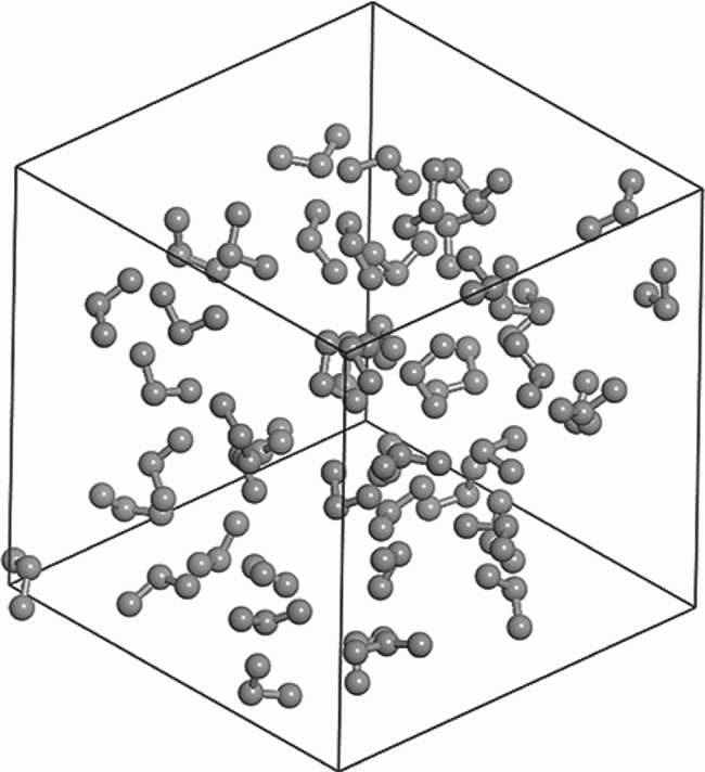
For a particle system, take molecules and atoms as examples. As shown in Figure 1, the atoms in the molecule system are collected with certain bonds in a spatial arrangement order. The atoms are considered to be the fundamental constituent particles in a molecule system, and are surrounded by other atoms (Pauling, Reference Pauling1988). RDF of a specified atom in the molecule can express the densities of other atoms at different distances. It is obtained by calculating the number of atoms in the thickness of a spherical shell of Δ r with a distance of r from the specified atom i (McQuarrie, Reference McQuarrie1976), as expressed below:
Illustration of molecule and atoms.

 \begin{equation} g_i (r) =\frac{N_i ({r,\Delta r}) }{\rho V ({r,\Delta r})} \end{equation}
where g i(r) refers to the radial distribution of atom i at a distance of r, and N(r, Δr) refers to the number of atoms in the thickness of the spherical shell of Δ r with a distance of r from the central atom i. Δ r can be set randomly, but it should be noticed that the smaller Δ r is, the more precise the results will be. Δ r is usually obtained by dividing the radius of the molecule space R c by the set number of bins N g. ρ refers to the density of atoms in the molecule system, and can be obtained by dividing the number of atoms N by the volume of the molecule space V, so V(r, Δr) = 4πr 2Δr refers to the volume of the spherical shell.
In other words, RDF is capable of quantifying the local density of atoms in the molecule at different distances and expressing the distribution probability of atoms. Likewise, for the entire molecule, RDF can be calculated by accumulating all the densities of different atoms at different distances, which is expressed below:
 \begin{equation} g\left( r \right)=\mathop \sum \limits_i^N \frac{N_i \left( {r,\Delta r} \right)}{(1/2)N\rho V\left( {r,\Delta r} \right)} \end{equation}
where g(r) refers to the radial distribution of all atoms at a distance of r, and N refers to the number of atoms in the molecule. For simplicity of computation, half of the pairs of atoms have been skipped in the accumulating process of N i(r, Δr) because, for a pair of atoms, the distance from atom 1 to atom 2 is the same as the distance from atom 2 to atom 1. The denominator is multiplied by 1/2 because half of the pairs of atoms have been skipped in the accumulating process.
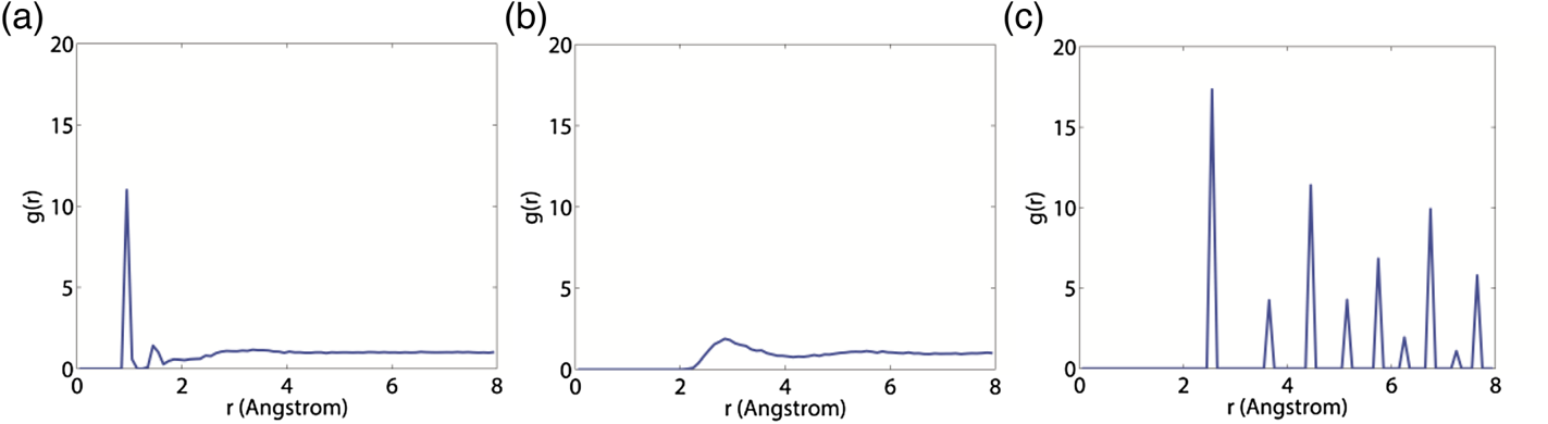
The RDF of the molecule is capable of describing the distribution probabilities of all the atoms inside it at different distances. Figure 2(a) gives the RDF graph of the example molecules (H2O molecules) in a unit cell. The x-axis in the graph represents the distance from the specified atom. It is suggested that there are several peaks of different shapes with the increase in distance. The height of peaks can express the distribution probability positively, namely the local density, of atoms in such a distance.
RDF graphs of (a) H2O (b) CO2 (c) Cu.

In addition, the integral of the curve can represent the overall distribution probability of atoms in the molecule system, which is called the coordination number in molecular dynamics. It refers to the number of particles directly linked to the specified particle in a particle system (IUPAC, 2014). In other words, it can determine the overall density around a particle. For example, the metal atoms are tightly stacked and result in a relatively high or even the highest coordination number (Bauer et al., Reference Bauer, Birk and Marks2009). The coordination number of a molecule can be obtained by the following equation:
 \begin{equation} L = \int_0^r {\mathop \sum \limits_i^N \frac{N_i ({r,\Delta r}) }{(1/2)N\rho V({r,\Delta r}) }dr} \end{equation}
where L is the average coordination number of the molecule.
Besides representing density distribution, RDF can also be employed to observe the order of particle distribution (Ma et al., Reference Ma, He, Xie, Zhu and Ma2019). As shown in Figure 2(a), some of the peaks are sharp while others are smooth. The sharp peaks indicate that the atoms distributed at such distances are relatively ordered. In contrast, the smooth peaks indicate disorderly distribution. On the whole, the atoms in a gas molecule have the most disorderly distribution for its characteristics (Bauer et al., Reference Bauer, Birk and Marks2009). As shown in Figure 2(b), the RDF graph of a gas molecule exhibits many smooth peaks, which suggests that the distribution probabilities of atoms in any distances are slightly different from each other, and the curve is close to a straight line. In contrast, for an ideal crystal molecule, the distribution of atoms is extremely well ordered (Chandler, Reference Chandler1987). The RDF graph of a crystal molecule, given in Figure 2(c), exhibits many sharp peaks, revealing that atoms are distributed in fixed positions. As a result, the order of distribution of atoms can be evaluated by analysing the RDF graph, which can be used to study the state of a substance.
3. DYNAMIC DENSITY MODEL
Ship density is a basic measurement in marine traffic. To overcome the limitations of the traditional concept of ship density, a new ship density model is proposed, termed dynamic density, which is composed of dynamic ship density in microscopic perspective and dynamic traffic density in macroscopic perspective.
3.1. Dynamic ship density
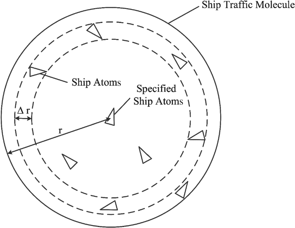
RDF is applied to dynamic density modelling as it can be used to study the density and order of particles. Thus, the ship traffic should first be converted to a particle system. A particle system is composed of large numbers of constituent particles. Hence, ship traffic may be considered as a particle system, with ships as its fundamental constituent particles. As shown in Figure 3, ship traffic is defined as the ship traffic molecule with ships as the atoms.
Illustration of ship traffic molecule and ship atoms.

In contrast with a particle system distributed in three-dimensional space, ship traffic is in two-dimensional space because ships are sailing on the water surface. As set out above, in a particle system, RDF can represent the distribution probability of particles by calculating the number of particles in a given thickness of a spherical shell with a given distance from the specified particle. However, in a two-dimensional ship traffic molecule system, the spherical shell does not exist. Hence, it should be converted to a two-dimensional circular ring. RDF of the ship traffic molecule can represent the distribution probability of ship atoms by calculating the number of ship atoms with a given width of a circular ring and a given distance from the specified ship atom, as shown in Figure 3. For a ship atom, RDF can represent the distribution probabilities of other ship atoms around it, as expressed in the following equation converted from Equation (1).
 \begin{equation} g_i (r) =\frac{N_i ({r,\Delta r}) }{\lambda \rho S({r,\Delta r}) } \end{equation}
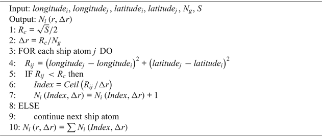
where g i(r) refers to the radial distribution of ship atom i at a distance of r, and N i(r, Δr) refers to the number of ship atoms in the width of a circular ring of Δ r with a distance of r from the specified ship atom i. ρ refers to the density of ship atoms in the ship traffic molecule system, and can be obtained by dividing the number of ship atoms N with the molecule area S. S(r, Δr) = 2πrΔr refers to the area of the circular ring, and λ is an adjusted coefficient. N i(r, Δr) can be obtained according to the algorithm shown in Algorithm 1.
Calculating N i(r, Δr)

Δr is obtained by dividing the radius of the S molecule area R c by the number of bins N g, and the radius R c will be divided into N g bins. Then, for each ship atom, the distance between other ships R ij should be calculated, and those within the molecule area S should be reserved. For each ship atom reserved, the bin index is identified by dividing exactly the distance R ij by Δr, and the ship atom will be accumulated in the corresponding bin. After accumulating all ship atoms, N i(r, Δr) can be obtained by accumulating the ship atoms in all bins.
Through the RDF graph, the local densities of ships at different distances can be obtained. To quantify the overall density around the ship, RDF was integrated with distance r. For a particle, the integration of RDF can represent the overall distribution probabilities of the surrounding particles. Similar to the particle, for a ship atom in the ship traffic molecule the overall density of other ship atoms surrounding it, namely the coordination number of the ship atom, can also be obtained by integrating its RDF. As coordination number can indicate the overall density, the coordination number of a ship atom is considered as dynamic ship density (DSD) in this paper. Thus, DSD is defined as the coordination number of a ship atom in the ship traffic molecule to reflect the density and compactness of other ships surrounding it.
The DSD of a ship atom i (DSDi) can be expressed as follows:
 \begin{equation} \mbox{DSD}_i =L_i = \int_0^r {\frac{N_i ({r,\Delta r}) }{\lambda \rho S({r,\Delta r}) }} dr = \int_0^r {\frac{N_i ({r,\Delta r}) S}{2N\lambda \pi r\Delta r}} dr \end{equation}
where L i refers to the coordination number of the ship atom i.
After obtaining all the DSDs in a ship traffic molecule, the distribution of DSDs was mapped by using the space interpolation technique. Interpolation is a technique whereby a continuous function is interpolated based on discrete data to make a continuous curve pass through all given discrete data points. Space interpolation technique is the application of the interpolation technique for a spatial purpose. It is used to convert the measurement data of discrete points in space to a continuous data surface. The method used in this study is spline interpolation, which makes a smooth curve passing through a series of points with variable splines (Hall and Meyer, Reference Hall and Meyer1976). Density mapping provides the opportunity to analyse visually and understand the patterns and behaviour of ship traffic (Aronsen, Reference Aronsen2017).
3.2. Dynamic traffic density
Similar to its operation in a particle system, RDF can obtain not only the distribution probabilities of ship atoms surrounding the specified ship atom, but also the overall distribution probabilities of all the ship atoms in the ship traffic molecule. Distribution probabilities of all ship atoms at different distances can be accumulated to obtain RDF of the ship traffic molecule, which is expressed as follows:
 \begin{equation} g\left( r \right)=\mathop \sum \limits_i^N \frac{N_i \left( {r,\Delta r} \right)}{(1/2)\lambda N\rho S\left( {r,\Delta r} \right)} = \mathop \sum \limits_i^N \frac{N_i \left( {r,\Delta r} \right)S}{\lambda N^2 {\pi} r \Delta r} \end{equation}
where g(r) refers to the radial distribution of all ship atoms at a distance of r.
The radial distribution of the ship traffic molecule can represent the local densities of ships at different distances in the ship traffic. To quantify the overall density of ship traffic, RDF was also integrated with distance r. The result is the average coordination number of the ship atoms in the ship traffic molecule. As the coordination number can indicate the overall density, it is considered as dynamic traffic density (DTD) in this paper, and is expressed as follows:
 \begin{equation}\mbox{DTD} = L = \int_0^r {\mathop \sum \limits_i^N } \frac{N_i ({r,\Delta r}) }{\frac{1}{2}\lambda N\rho S({r,\Delta r}) }dr = \int_0^r {\mathop \sum \limits_i^N } \frac{N_i ({r,\Delta r}) S}{\lambda N^2{\pi }r\Delta r}dr \end{equation}
DTD refers to the average coordination number of the ship atoms in the ship traffic molecule, representing the overall density and compactness of the ship traffic.
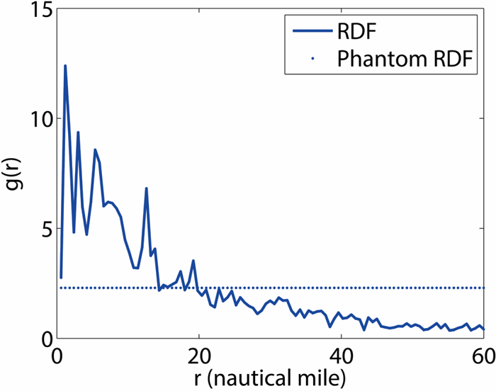
Apart from representing distribution of density, RDF can also be employed to study the order of particle distribution, as stated in Section 2. For example, the RDF graph of the ship traffic molecule is shown in Figure 4. In order to evaluate the order of ship positions in ship traffic, a new method was proposed by using the RDF of the ship traffic molecule. As stated in Section 2, smooth peaks in the RDF graph indicate disorderly distribution. Therefore, the extreme circumstance of disorder for the graph is a straight line. Thus, a phantom straight line was assumed to represent the RDF of the extremely disordered state. The phantom straight line, combined with the original RDF graph, is also shown in Figure 4. It was assumed that the order can be represented by the deviation from the phantom straight line. It is considered as dynamic traffic order (DTO) in this paper, which can indicate the order of distribution of ship atoms in the ship traffic molecule, and also represent the order of ship positions and the complexity of ship traffic to some extent.
RDF graph of the ship traffic molecule.

DTO can be obtained by the following equation:
 \begin{equation} \mbox{DTO}=\frac{1}{N}\sum \left( {\mathop \sum \limits_i^N \frac{N_i ({r,\Delta r}) }{(1/2)\lambda N\rho S({r,\Delta r}) }-p} \right)^2=\frac{1}{N}\sum \left( {\mathop \sum \limits_i^N \frac{N_i ({r,\Delta r}) S}{\lambda N^2\pi r\Delta r}-p} \right)^2 \end{equation}
where p refers to the value of the phantom straight line.
4. CASE STUDY
4.1. Selection of studied water areas and data
AIS is a new information and telecommunication navigation aid system which is applied in maritime safety and communication between ship and shore and between ship and ship. It can automatically broadcast important shipping information via very high frequency (VHF) to ships and coast stations nearby (Kokotos et al., Reference Kokotos, Linardatos, Nikitakos and Tzannatos2010,Reference Kokotos, Linardatos, Nikitakos and Tzannatos2011). The application of AIS is conducive to enhancing the safety of life at sea and improving the safety and efficiency of navigation.
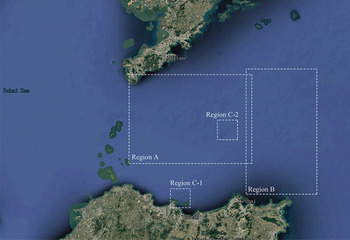
Real AIS data were decoded and interpolated to validate the proposed model. The water area selected for validation was around Bohai Strait, including Bohai Strait and the northern Yellow Sea area east to Bohai Strait, as shown in Figure 5. Bohai Strait is one of the three major straits in China, connecting the Bohai Sea and the Yellow Sea. The selected water area features high ship density and complex traffic situations. Compared with the other two major straits in China, the Taiwan Strait and the Qiongzhou Strait, the selected water area has its merits in traffic volume and traffic pattern for validation.
The studied water area in Bohai Strait.

4.2. Validation of DSD
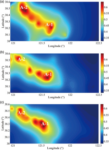
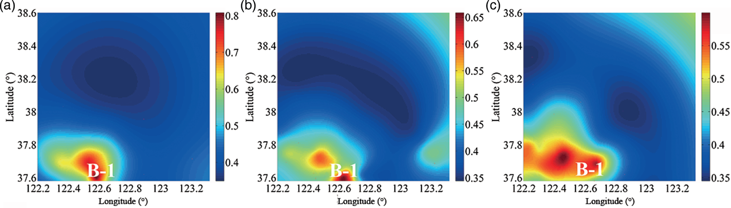
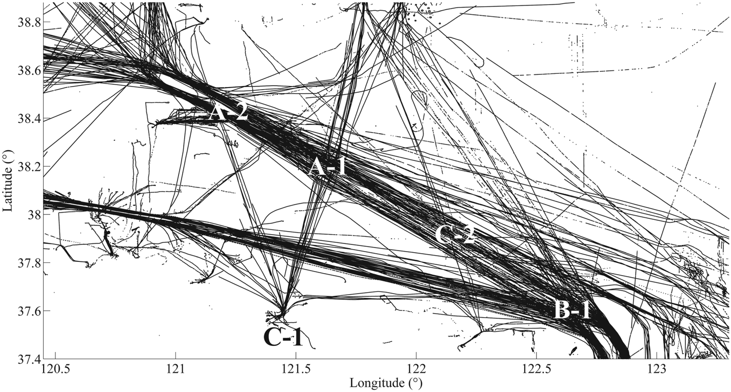
Regions A and B in the studied water area were used for validating DSD by density mapping. For each region, three different moments were chosen: 16:00, 16:30 and 17:00 on 27 July 2018. DSD maps are shown in Figures 6 and 7. For Region A, it can be seen that two regions around 38.3°N 121.5°E and 38.5°N 121°E have high density, marked as A-1 and A-2 respectively. To evaluate the effectiveness of DSD, a ship trajectory map of the studied water area is depicted for comparison, shown in Figure 8. It is observed that in Region A-1, two main traffic flows encounter one another in the studied water area. This leads to relatively high ship density and compactness, which is in line with the results in the DSD maps. Region A-2 is the eastern entrance and exit of the Lao Tieshan Traffic Separation Scheme (TSS). Ships passing the TSS meet in this region, causing high ship density and compactness, which is also indicated by the density maps. In Region B, the region of high density is around 37.6°N 122.6°E, marked as B-1. As shown in the ship trajectory map, Region B-1 is filled with ship trajectories, indicating high ship density and compactness. Traffic flows meet in Region B-1 close to Chengshanjiao Precautionary Area, which is the eastern entrance and exit of the studied water area. In addition, Region B-1 is close to Weihai Port. Therefore, ships near Weihai Port are more likely to encounter traffic flows there, resulting in high ship density and compactness. This finding is also consistent with the results in the DSD maps.
DSD maps of Region A.

DSD maps of Region B.

Map of ship trajectories in the studied water area for 24 h.

4.3. Validation of DTD
To validate dynamic density from the macroscopic perspective, another two regions were studied, marked as C-1 and C-2. Region C-1 refers to the water area near Yantai Port, located at 37.5°N to 37.75°N, 121.25°E to 121.5°E approximately. Region C-2 refers to the water area northwest of Chengshanjiao Precautionary Area, located at 38.0°N to 38.25°N, 121.75°E to 122.0°E approximately. The water area around Region C-2 is relatively open.
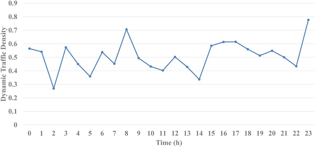
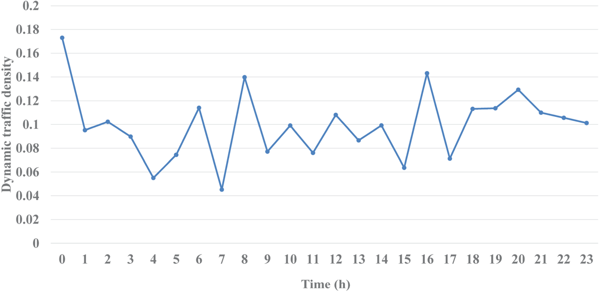
Using the proposed model, DTD for the two regions can be expressed. DTD variation for the two regions over 24 hours on 27 July 2018 is illustrated in Figures 9 and 10, in which an initial instantaneous moment was selected to represent each hour.
DTD of Region C-1 in 24 h.

DTD of Region C-2 in 24 h.

It can be observed that the DTDs of Region C-1 are noticeably greater than those of Region C-2, suggesting that the density and compactness of ships in Region C-1 is higher than those in C-2. To assess the compactness quantitatively, the mean distance between ships was adopted as an indicator, as it is negatively correlated with ship compactness. The mean distance between ships (Meandis) can be expressed as follows:
 \begin{equation} \mbox{Meandis}=\frac{1}{N^2}\mathop \sum \limits_{i=1}^N \mathop \sum \limits_{j=1}^N \sqrt {({\mbox{long}_i -\mbox{long}_j }) ^2+({\mbox{lat}_i -\mbox{lat}_j }) ^2} \end{equation}
where longi, lati, longj and latj refer to the longitude and latitude of Ship i and Ship j.
To express the overall density and compactness of each region, the average values of DTD for each hour are given in Table 1, together with the average value of Meandis for each hour. The negative correlation between DTD and Meandis is significant, thereby proving that DTD can represent the density and compactness of ships effectively. Moreover, it is known that port areas always have relatively high ship density due to their large trade volume and the limited navigation conditions (Debnath and Chin, Reference Debnath and Chin2016). As a result, the density and compactness of ships in the port area should be greater than for other, wide open water areas, which can be proved by the results in Table 1, representing that the results of the experiment are consistent with the real-world situation.
Average values of DTD and Meandis in Regions C-1 and C-2.

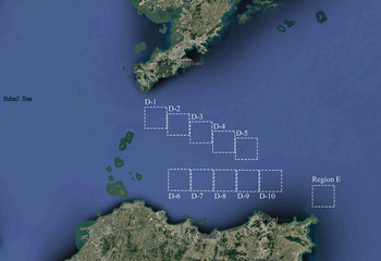
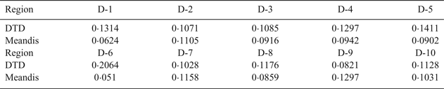
In addition, another 10 regions were selected and marked as D-1 to D-10, as shown in Figure 11. DTDs for these 10 regions are listed in Table 2, in which Meandis is also presented.
Illustration of Region D and Region E.

DTD, Meandis for Regions D-1 to D-10.

To validate the results, a Pearson correlation analysis was carried out. The correlation coefficient between DTD and Meandis was –0.856, the absolute value of which was between 0.8 and 1.0, and the P value was less than 0.01, indicating the strong negative correlation between them.
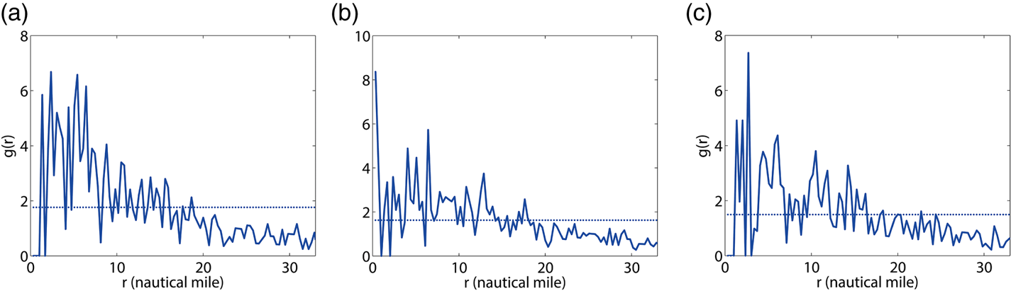
Regions A and B were used for validating the DTO. The results for the different moments are shown in Table 3, and the RDF graphs for the two regions are illustrated in Figures 12 and 13. It can be observed that the orders of Region A are obviously greater than those in Region B. The results can be explained by the characteristics of the two regions, where Region A is mainly composed of traffic flows, as shown in Figure 8, and Region B is mainly composed of the Precautionary Area and ports. Normally, ships in traffic flows are relatively well ordered because their courses and routes are relative fixed (Yip, Reference Yip2013). In contrast, ships in the Precautionary Area and ports are relatively disordered as their courses and routes are varied. Figures 12 and 13 can also explain the results. It can be found that the distribution probabilities of ships in Region A remain large at distances of less than 12 nautical miles and become small at distances of more than 12 nautical miles, indicating that the distances between ships are relatively fixed. For Region B, it can be found that the large distribution probabilities do not obviously focus on any distance, indicating that the distances between ships in Region B are various.
RDF graphs of Region A.

RDF graphs of Region B.

DTO of Regions A and B.

5. DISCUSSION
The proposed dynamic density model was based on RDF in molecular dynamics. To emphasise the novelty and advantage of the proposed model, a comparison between the proposed model and the traditional density modelling in a previous study was carried out. The selected traditional model is the vessel density model (Wu et al., Reference Wu, Xu, Wang, Wang and Xu2017), which is defined as the number of vessels per unit area for a moment. This density modelling method is also used in many other previous studies of ship density (Baladacci and Carthel, Reference Baladacci and Carthel2009; MMO, 2014; Aronsen, Reference Aronsen2017).
To compare the proposed model with the traditional density model in terms of compactness identification, several pairs of scenarios were selected in Region E, shown in Figure 11. The number of the pairs which can reflect negative correlation between DTD and Meandis was counted and it was the same as for the traditional density model. The results shown in Table 4 indicate the great advantages of DTD in compactness identification.
Counts of effective compactness identification.

In addition, to emphasise the difference between the proposed model and the traditional density model, some scenarios were simulated in the studied water area, as shown in Figure 14. The related results are listed in Table 5. The five scenarios possess the same number of ships, indicating that the density for the five scenarios will also be the same as when adopting the traditional density model. However, the Meandis values decrease from Scenario 1 to Scenario 5, indicating that the ships become increasingly compact, which the traditional density model is unable to reflect, while DTD values increase in a gradual manner, and can effectively represent the change of compactness of these scenarios. This is because the proposed model identifies density based on the relative distance between ships, while the traditional model calculates the density only by counting the number.
Five simulated scenarios with different levels of compactness.

Comparison between DTD and the traditional density model.

In addition to the advantage in compactness identification, the proposed model also has advantages in complexity identification. Five other scenarios were simulated, as shown in Figure 15. Among the five scenarios, the order of the first four scenarios decreases gradually. In order to quantify the order, the number of ordered ships (NOS), namely the number of ships with the same distance apart, was adopted as an indicator. The lower the NOS, the less the order will be. The related results are listed in Table 6.
Five simulated scenarios with different levels of order.

Comparison between DTO and the traditional density model.

It can be observed that the five scenarios possess the same ship density according to the traditional density model. However, NOS becomes less and less for the first four scenarios, indicating that the complexity of the ship traffic increases. As shown in Table 6, DTO obtained from the proposed model of the first four scenarios also decreases, which is in line with the orders of the four scenarios, indicating that the proposed model can represent the order of ship positions and reflect the complexity of ship traffic to some extent, while the traditional density model is unable to reflect this. Compared with the traditional model, which is based on the counting of ships, the proposed model can utilise the characteristic of RDF to reflect the complexity of ship traffic to some extent.
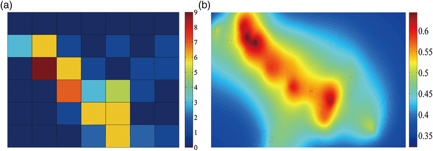
The proposed model can also map the ship density with greater precision compared with the traditional density model. Ship density maps obtained by the traditional density model are normally depicted by the gridding method (MMO, 2014; Wu et al., Reference Wu, Xu, Wang, Wang and Xu2017). Figure 16 shows the ship density map obtained by the traditional density model for Region A in the studied water area combined with the density map obtained by the proposed model. It can be clearly seen that the precision in the proposed map is greater, while the ship density and compactness of each grid can only be determined roughly in the traditional map. The resolution of the density map from the traditional density model was 7? × ?6, compared with 200? × ?200 in the density map for the proposed model; hence the resolution of the density map obtained from the proposed model is significantly improved compared with the traditional one. Compared with the traditional density mapping, which maps the density by a series of regions, the proposed model can map the density to the precision of a point.
Density maps based on (a) the traditional model; (b) the proposed model.

In the proposed model, DTO is somewhat limited when there are very few ships or when ships are extremely close in distance, as the deviation between the RDF curve and the phantom straight line cannot be represented accurately in such situations. In addition, though DTO in the proposed model can reflect the complexity of ship traffic to some extent, it should be noticed that DTO can only reflect the complexity of ship traffic from a macroscopic perspective, which is the complexity in distribution of ship positions. In traffic complexity modelling, in addition to the distribution of vehicle positions, some factors in microscopic perspective should also be considered, such as heading change, speed change, altitude change, etc. in air traffic complexity (Laudeman et al., 1998), and crossing angle, relative motion, degree of convergence, etc. in marine traffic complexity (Wen et al., Reference Wen, Huang, Zhou, Yang, Xiao and Wu2015). Therefore, to reflect the complexity of ship traffic more accurately, other microscopic factors should be considered together with DTD and DTO.
In addition, the molecular collision theory is widely used in modelling collision probability in maritime traffic (Fujii and Tanaka, Reference Fujii and Shiobara1971; Macduff, Reference Macduff1974; Pedersen, 1995; Altan and Otay, Reference Altan and Otay2018). According to this theory, a collision will happen if the distance between the centres of particles within a domain is equal to the collision diameter (Altan and Otay, Reference Altan and Otay2018). Similar to the molecular collision theory, the molecular dynamic approach proposed in this paper also uses distance between ships as a crucial variable in the RDF modelling. Therefore, the molecular dynamic approach and the molecular collision theory can be complementary to each other. For future work, the proposed approach could be extended by combining it with the molecular collision theory.
6. CONCLUSION
In the present study, a dynamic density model based on RDF was proposed. The density and the complexity of ships were expressed by analysing the RDF of ship atoms in a ship traffic molecule. From the microscopic perspective, the model is capable of identifying the density and compactness around each ship based on DSD and then mapping the ship density distribution. From the macroscopic perspective, the model can identify the global density and compactness of ships in ship traffic and the order of ship positions based on DTD and DTO, respectively, thereby to some extent reflecting the complexity of ship traffic. Real AIS data of the Bohai Strait area was employed to verify the feasibility of the proposed model. According to the results, the proposed dynamic density model can express the density and complexity of ships effectively.
The proposed model, based on instantaneous values varying with time, demonstrates dynamic characteristics. Compared with the limitations of the traditional ship density model, the proposed model can identify compactness and complexity more effectively and accurately. In addition, the proposed model successfully maps the distribution of ship density with greater precision.
The proposed dynamic density model is capable of assisting the work of marine surveillance operators. With DSD in the proposed model, density mapping of ships can be achieved more precisely, which helps operators perceive the distribution of ship density in a clear manner by visually analysing and understanding the patterns and behaviours of the ship traffic. DTD and DTO in the proposed model can provide a global metric for maritime traffic and provide the traffic information for decision making. In particular, the complexity of ship traffic expressed by DTO can be adopted to investigate maritime traffic patterns and support maritime surveillance operators to improve their traffic situation awareness, helping them comprehend the traffic situation and organise the ship traffic better. In other words, it can be conducive to the operations of vessel traffic services (VTS) and assist the VTS operators to gain a better awareness of the traffic situation when planning traffic activities and monitoring the ship traffic in the VTS area, which helps to prevent the formation of dangerous situations and improves the safety of maritime traffic. Similar to the complexity application in air traffic, the metric can also be adopted to assess the workload of marine surveillance in combination with other indicators. Additionally, the metric can be employed to analyse the ship traffic patterns and the collision risk in VTS area and used as a reference by administrators for relevant decision making.
In modelling DTO in this study, ship position was the only factor to be considered. As a result, DTO can only represent the complexity of ship traffic to some extent. In the real world, microscopic factors such as course, speed, etc. could also influence the complexity of ship traffic. In order to represent the complexity of ship traffic more accurately, these factors can be incorporated into the model in future research. In addition, since the molecular dynamic approach and the molecular collision theory can be complementary to each other, the proposed model can be extended with the molecular collision theory in future work.
ACKNOWLEDGEMENTS
The authors would like to express gratitude to the editors and reviewers whose valuable comments and suggestions will make contribution to improvements of the quality of this paper.
CONFLICT OF INTEREST
None.