





Nomenclature
-
 ${a_X}$
,
${a_Y}$
,
${a_Z}$
-
translational accelerations in the body coordinate system
-
${\rm{BVLOS}}$
-
beyond visual line of sight
-
${\rm{CFD}}$
-
computational fluid dynamics
-
${C_{L,0}}$
,
${C_{D,0}}$
-
lift and drag coefficients at zero angle-of-attack
-
$C{l_{\delta L}}$
-
aileron effectiveness coefficient
-
$C{m_{\delta M}}$
-
elevator effectiveness coefficient
-
${\rm{CG}}$
-
centre of gravity
-
${\rm{CS}}$
-
certification specifications
-
${\rm{EASA}}$
-
European Union Aviation Safety Agency
-
${\rm{EKF}}$
-
extended Kalman filter
-
${\rm{FCS}}$
-
flight control system
-
$g$
-
acceleration due to gravity
-
${\rm{GNSS}}$
-
Global Navigation Satellite System
-
$h$
-
geodetic altitude
-
${\rm{HTP}}$
-
horizontal tail plane
-
${\rm{IMU}}$
-
inertial measurement unit
-
${\rm{IPS}}$
-
icing protection system
-
${\rm{lat}}$
,
${\rm{lon}}$
,
$h$
-
latitude, longitude and altitude in the geographic coordinate system
-
${\rm{LTI}}$
-
linear time-invariant
-
${\rm{MVD}}$
-
median volume diameter
-
${\rm{PID}}$
-
proportional integral derivative
-
${\rm{SAE}}$
-
Society of American Engineers
-
${\rm{TAS}}$
-
true airspeed
-
${\rm{TECS}}$
-
total energy control system
-
$u$
,
$v$
,
$w$
-
translational velocities in the body coordinate system
-
${u_A}$
,
${v_A}$
,
${w_A}$
-
translational velocities in the wind coordinate system
-
${\rm{UAV}}$
-
unmanned air vehicle
-
$p$
,
$q$
,
$r$
-
roll, pitch and yaw rates
-
${\rm{po}}{{\rm{s}}_N}$
,
${\rm{po}}{{\rm{s}}_E}$
-
position in the local-level coordinate system
-
${V_N}$
,
${V_E}$
,
${V_D}$
-
translational velocities in the local-level coordinate system
-
${x_{CG}}$
-
centre of gravity longitudignal position


Greek symbol
-
$\alpha $
-
angle-of-attack
-
$\beta $
-
angle of sideslip
-
$\gamma $
-
flight path angle
-
${\delta _L}$
,
${\delta _M}$
,
${\delta _N}$
-
ailerons, elevator and rudder deflection angles
-
$\theta $
-
pitch angle
-
$\tau $
-
throttle fraction
-
$\phi $
-
bank angle
-
$\chi $
-
course angle
-
$\psi $
-
heading angle


Subscripts
-
${\rm{SIM}}$
-
simulation model
-
${\rm{FIT}}$
-
fitted model
- r
-
reference signal
- d
-
disturbance signal


1.0 Introduction
Small fixed-wing unmanned aerial vehicles (UAVs) have become instrumental in collecting affordable aerial images for military or civilian purposes. However, the threat of icing severely restricts their employment in regions subject to cold climates [Reference Sørensen1]. Platform-specific effects typically include higher droplet collection efficiency compared to manned aircraft and more severe aerodynamic penalties due to ice accretions at low Reynolds numbers [Reference Hann and Johansen2]. Although comprehensive icing protection systems (IPS) are being developed [Reference Hann3] to allow flight into known icing, their size, weight and power footprint may not be justified for operations under moderate icing risk. Hence, there is a need for a compromise solution that restores some level of operational capability while reducing the penalties associated with an extensive IPS.
This work introduces the concept of a sense-and-egress module designed to trigger and execute an escape manoeuvre, allowing the UAV to exit the icing conditions before the performance and flying qualities of the platform degrade to a critical level. The first part details the operating principles of the system and proposes a suitable architecture. The benefits and drawbacks of the proposed solution are assessed with respect to alternative solutions. Enabling technologies and knowledge gaps are briefly explored in order to gauge the maturity of the concept. In the second part, the flight dynamics model of the PX-31 Falk UAV is derived from numerical simulations and experimental data. An emphasis is put on tailoring and validating the model structure using system identification from flight tests. In the third section, a synthesis and simulation framework is developed to tune the platform’s guidance and control laws. The selected autopilot architecture is detailed, as well as the frequency- and time-domain analysis of the two main controllers. An assessment of the effects of icing on the autopilot trajectory is provided in the case of a simple egress manoeuvre. A permanent elevator limiter and an adaptive bank angle limiter are added to address the shortcomings of the baseline autopilot. Special attention is given to the compromise between reduction of trajectory excursions and minimisation of manoeuvre completion time, as well as the preservation of gust resistance capabilities.
2.0 The sense-and-egress concept
The purpose of the sense-and-egress module is to fill the capability gap between unprotected and fully ice-protected UAVs by increasing the chance of platform survival in case of an inadvertent icing encounter. In that case, the module initiates and conducts an escape manoeuvre to attempt to save the platform. This is a key difference with respect to IPS, which are designed to ensure safe flight into and through known icing conditions, offering greater capability at the cost of extensive hardware integration. IPS have been adopted by most commercial or military aircraft and are currently being developed for small UAVs. However, there is a need for more frugal solutions suitable for environments presenting a limited icing risk or platforms unable to bear the performance penalties due to IPS. Compared to legacy UAVs without ice protection, the platforms equipped with sense-and-egress technology should benefit from greatly improved survivability in icing conditions thanks to timely ice detection, protection of critical components and adequate mitigation strategies. This would enable a shift in operational perspective and risk assessment: The no-go criteria associated with atmospheric conditions could be significantly relaxed, with a consequent increase in availability and profitability.
2.1 Operating principles
The sequence of actions performed by the sense-and-egress may be more or less extensive, as a result of the trade-off between performance and complexity. The most elaborate sequence consists of the following steps:
-
1. Detection of ice accretion
-
2. Estimation of current and future flight envelopes
-
3. Generation of a suitable egress manoeuvre (trajectory and constraints on flight variables)
-
4. Manoeuvre execution: tracking of trajectory under flight variable constraints
Note that the flight performance of the platform is to be continuously monitored during the execution of the manoeuvre. If, at any instant within the flight envelope prediction horizon, the trajectory tracking problem becomes unfeasible, the remote pilot may be prompted to relax constraints on the egress manoeuvre. Conversely, the manoeuvre may be terminated if monitoring shows that the flight performance of the platform has recovered.
2.2 Technical description
The main function of the sense-and-egress system can be performed by a set of interconnected modules, each of them with a specific purpose. The chart shown in Fig. 1 suggests a decomposition of the system containing four main modules and two optional ones. The function of each main module can be summarised as follows:
-
• The flight condition monitoring tracks the evolution of the flight variables to quantify performance degradation and detect ice accretion. The performance indicators to be monitored and fed to the flight envelope prediction algorithm include the power imbalance (icing-induced change of total energy) proposed by Deiler and Fezans [Reference Deiler and Fezans4]. This quantity is used to implement an indirect ice detection method, which can be supplemented by external sensor data to improve sensitivity and reliability [Reference Sachs, Schwarz and Deiler5].
-
• The flight envelope prediction module estimates the current operating limits based on the performance deltas provided by the monitoring routine. The purpose of this module is to allow the guidance and control laws to operate closer to the platform lift and power limits in order to speed up its exit from hazardous conditions. The evolution of those limits is forecasted over a relevant time horizon to anticipate further performance degradation while the egress manoeuvre is already in progress.
-
• The guidance law commands the flight variables to perform a safe evasive manoeuvre, accounting for degrading operating limits. Its goal is to minimise exit time under performance and control constraints. Terrain data provided by an additional module could be used to better exploit the potential energy of the platform.
-
• The control law drives the flight variables to follow guidance commands and reject disturbances in spite of model uncertainties. The performance of the control loop conditions the quality of the trajectory tracking.
Architecture of a sense-and-egress system.

Figure 1. Long description
The flowchart illustrates the architecture of a sense-and-egress system for an unmanned air vehicle. The process begins with inputs from an ice sensor and a terrain awareness module. The ice sensor provides ice accretion severity data to the flight condition monitoring system. The terrain awareness module provides terrain clearance estimates to the guidance law. The flight condition monitoring system sends performance deltas to the flight envelope prediction system. The flight envelope prediction system uses these performance deltas and sensor outputs from the UAV to determine flight envelope bounds, which are then sent to the guidance law. The guidance law uses these bounds along with the flight states reference from the terrain awareness module to generate control inputs. These control inputs are sent to the control law, which then controls the UAV. The UAV sends sensor outputs back to the flight envelope prediction system, creating a feedback loop.
2.3 Complementarity with other icing protection concepts
This section addresses the key differences and similarities between sense-and-egress and IPS. From an implementation standpoint, the main difference between the two systems lies in the extent of the protected components. The sense-and-egress only requires protection of the critical components, which are the most vulnerable to icing (i.e. the air data probes and propellers). The IPS, however, needs to provide deicing or anti-icing action on the lifting surfaces such as the wings and horizontal tail. This can be accomplished through a variety of thermal, mechanical or chemical means. The actions taken also differ according to the purpose of the system and its installed hardware: In the IPS case, the availability of extensive deicing or anti-icing hardware allows for the planned flight path and focus on mission completion. In the sense-and-egress case, the lack of comprehensive icing countermeasures prompts the system to abort the flight plan and perform an evasive manoeuvre in order to focus on platform survival. Hence, compared to IPS, sense-and-egress may offer the following advantages:
-
• Reduced performance penalties outside of icing conditions: The weight penalty associated with wing and tail de-icing systems is avoided, which may be significant when the aspect ratio of those lifting surfaces is high.
-
• Reduced unit cost: The above-mentioned systems may represent a significant fraction of the platform cost or require a more complex manufacturing process.
-
• Improved reliability: A lower number of non-redundant systems implies a lower probability of failure. De-icing systems, which are integral to the airframe, may be less serviceable than other components.
-
• Availability and scalability: As the few ice-protected components required by the sense-and-egress are not part of the airframe, they may be retrofitted to legacy platforms or even shared between a fleet of UAVs of the same type.
For all its merits, it may, however, present the following drawbacks:
-
• Broader development effort: As sense-and-egress heavily relies on the prediction of the platform flight dynamics and includes a flight control module, the development costs associated with modelling and control may be higher than for IPS. The interface requirements with the legacy platform autopilots may also generate additional complexity.
-
• More restrictive operational requirements: As this system does not allow flight into known icing, the range of atmospheric conditions in which UAV operations remain possible is more limited than for IPS.
-
• Loss of mission capability on an icing encounter: Since the platform is required to manoeuvre in order to survive an icing encounter, adherence to the initial flight plan can no longer be guaranteed, which may be unacceptable for time-critical scenarios. The energy expenditure due to evasive manoeuvres can be prohibitive and may require aborting the mission.
2.4 Enabling technologies and knowledge gaps
The aim of this section is to propose a brief overview of the relevant previous works in each of the topics that are crucial to the development of a sense-and-egress module.
2.4.1 Flight dynamics modelling
The approach explored by Deiler [Reference Deiler6] is to describe the dynamics of the iced aircraft as the sum of the dynamics of the clean aircraft and the contribution due to ice accretion. In the frame of this work, the base model of the clean UAV was obtained using computational fluid dynamics (CFD) [Reference Lindner, Wallisch and Hann7], panel methods [Reference Skogan8] and wind tunnel tests of the propulsion subsystem [Reference Løw-Hansen9]. The perturbation component has been computed from CFD simulations on insulated wing and tailplane aerofoil sections [Reference Lindner, Wallisch and Hann7]. The method detailed in Ref. [Reference Skogan8] uses a multiplicative scheme instead of the additive contribution implemented by Ref. [Reference Deiler6]. It must be noted that the applicability of this iced model is limited to a single case of atmospheric conditions with a given set of static temperature, liquid water content and droplet mean volume diameter values. The ice accumulation rate is assumed to be constant, with linear performance degradation up to the state corresponding to the maximum icing time.
As the topology of ice accretions and the severity of the resulting aerodynamic penalties strongly depend on the atmospheric conditions [Reference Hann10], which are not commonly monitored on board of small UAVs, the icing model should represent a worst-case scenario with regard to expected operating conditions. Local measurements of ice thickness provided by onboard ice sensors may be used to drive a multi-model strategy. which could allow to reduce the conservatism of this approach. The source data of the icing model could also be updated to include the recent icing wind tunnel campaign carried out with the wing aerofoil section [Reference Hann11]. Ultimately, the measurement of the forces and moments acting on the whole aircraft would yield an even more representative model of its flight dynamics in icing, but the associated costs and time expenditure would be significant.
2.4.2 Performance-based ice detection
This ice detection technology is based on the estimation of the rate of change of the total energy of the aircraft [Reference Deiler and Fezans4]. The in-flight estimated value is compared to the expected value known from the nominal aircraft model. Ice is detected when the difference exceeds a specific threshold, which is chosen as a compromise between detection sensitivity and false alarm rate. This methodology has recently been validated on business jets and large transport aircraft [Reference Deiler12]. However, its applicability to small UAVs remains to be proven as there may be less data available to build an accurate nominal aircraft model.
2.4.3 Flight envelope prediction
Two definitions of the flight envelope are proposed in the literature: the most extensive one is described as the manifold of the state space from the 6 degrees-of-freedom equations of motion [Reference Beard and McLain13] where the aircraft can remain controllable [Reference Zogopoulos-Papaliakos, Karras and Kyriakopoulos14]. The more computationally tractable one, also called the trim flight envelope, only includes the equilibrium points of the system. Those points are usually constrained by thrust and angle-of-attack (
 $\alpha $
) limitations, which may both be affected by icing. Modelling of
 $\alpha $
-induced aerofoil flow separation (stall) and its effect on aircraft flight dynamics has been carried out via a variety of methods, including system identification from flight test data [Reference Fischenberg and Jategaonkar15]. However, variants of this method compatible with real-time processing (i.e. online system identification) have failed to accurately capture stall phenomena observed on small delta-wing UAVs [Reference Saderla, Kim and Ghosh16]. This begs the question of whether or not online system identification methods could estimate the effects of icing on the flight envelope.
Assuming that the icing phenomenon could be captured, the data collected would only represent its influence on the current operating condition, which itself may be far from the flight envelope bounds. Thus, one could either adjust the operating condition, ultimately putting the UAV at risk, or infer the performance delta at the bound from its value at a safer operating point, creating potentially large uncertainties in the process. Prediction of the evolution of the operating limits may also not be straightforward, as the severity of icing buildup could depend on some of the flight variables, such as
 $\alpha $
, altitude or airspeed, which vary during the manoeuvre. Rough estimates could be obtained by extrapolating the data trend, but physics-based evolution laws should be sought to consolidate the predictions.
All that being said, flight envelope predictions may be inaccurate if available at all. Thus, the guidance and control laws should be designed to be able to perform the egress manoeuvre in the absence of accurate flight envelope bounds. It may also be wise to postpone the development of such methods until a baseline autopilot is implemented.
2.4.4 Guidance and control laws
Both guidance and control aspects of the autopilot are tightly coupled, as the bandwidth of the control law conditions the performance of the trajectory tracking loop. This is because it may be desirable to enforce time-scale separation between both loops. Under this assumption, the control and guidance gains can be tuned sequentially, starting with the inner (control) loop [Reference Beard and McLain13].
Robust synthesis techniques can be employed to guarantee closed-loop stability in the presence of model uncertainties [Reference de Aguiar, Apkarian and Noll17], which may be correlated with the performance deltas determined by the flight condition monitoring module. Structured
 ${{\cal H}_\infty }$
synthesis appears to be a suitable choice as it is able to balance performance, robustness and actuator usage objectives [Reference Apkarian18]. Moreover, it can be used on any prescribed controller structure, which simplifies its implementation both in simulation and on flight hardware.
Model predictive control is also of interest because of its ability to account for time-dependent constraints on the flight states [Reference Gavilan, Vazquez and Camacho19]. However, solving the online optimisation problem is often computationally intensive and may not always be feasible. Moreover, obtaining stability guarantees could be a challenge for such classes of systems [Reference Eren20].
3.0 Flight dynamics model of the Falk UAV
3.1 Platform description
The PX-31 Falk, pictured in Fig. 2, is a small fixed-wing UAV manufactured by the Norwegian company Maritime Robotics. Its maximum take-off weight is 22 kg for a payload of 7 kg and a wing span of 3.2 m. It is powered by an electric motor driving a pusher propeller up to a ceiling of 20.000 ft and a maximum airspeed of 40 m/s. This platform is capable of Beyond Visual Line Of Sight (BVLOS) operation thanks to a long-range very high frequency (VHF) radio link. As current operational limitations [Reference Hann and Trolle Borup21] preclude BVLOS operations when static ground air temperature drops below a given threshold, the availability of this platform could be greatly improved by providing protection against inadvertent icing. Hence, the Falk is a prime candidate for the application of sense-and-egress algorithms.
The Falk UAV on its launch rail; DLR (CC BY-NC-ND 3.0).

3.2 Baseline mixed-fidelity model
Both linear and non-linear formulations of the UAV flight dynamics model are required to, respectively, synthesise the control laws and assess the sense-and-egress autopilot in icing conditions. The baseline representation of the aerodynamic forces and moments is derived from the numerical works of Skogan [Reference Skogan8] including dynamic coefficients from the panel code XFLR5, as well as CFD-computed lift, drag and pitching moment polars originally published by Lindner et al. [Reference Lindner, Wallisch and Hann7]. This CFD dataset covers both the main wing and horizontal tail plane (HTP) aerofoil s for various icing conditions. For this work, the worst-case scenario has been chosen according to the most severe continuous maximum icing case (as defined by EASA CS-25 Appendix C) identified by Lindner [Reference Lindner, Wallisch and Hann7]. This scenario entails a static air temperature of −2° and a droplet median volumetric diameter (MVD) of 15
 $\mu {\rm{m}}$
with an accretion time of 21.5 min.
The model structure proposed by Skogan and adopted in this work resolves the longitudinal forces and moments at both the main wing and HTP centres of pressure while the lateral directional actions are applied at the vehicle centre of mass. This decomposition models the effect of the downwash induced by the wing on the HTP as well as the pitch damping effect provided by the tail. Both lifting surfaces have individual non-linear lift, drag and pitching moment polars, allowing wing stall, tailplane stall or any combination of those effects to be captured. Numerous general aviation accidents [Reference Ratvasky, Zante and Riley22, Reference Bromfield23] show that this level of detail is crucial for flight dynamics investigations in icing conditions. Note that the wing incidence angle of the Falk is 4°, giving a stall angle of respectively 7° and 4° for clean and iced configurations.
The propulsion system model is given by the experimental findings of Løw-Hansen [Reference Løw-Hansen9]. Note that the propeller is assumed to be ice-protected, hence remaining free from any performance degradation due to icing. Relevant terms of the inertia tensor are estimated from pendulum experiments performed by Løw-Hansen at the Norwegian University of Science and Technology. It is also assumed that the effect of ice accretion on the mass and inertia properties of the UAV is negligible. Finally, the formulation of the 6 degrees-of-freedom equations of motion is provided by Beard and McLain [Reference Beard and McLain13] with additions from Zipfel [Reference Zipfel24] regarding the quaternion formulation of the attitude angles and angular rates. The linear, time-invariant (LTI) forms of this model are obtained through a Jacobian linearisation performed under the assumption of steady-level flight.
3.3 Tailoring to flight test data
Even though the model structure has been selected to simulate the Falk dynamics in icing conditions with adequate fidelity, there may be significant deviations with respect to the behaviour of the actual platform. Hence, data from a functional check flight has been leveraged in an attempt to bridge this gap. The opportunistic nature of the test data leads to significant limitations in the analysis. The adverse factors detrimental to the accuracy of the system identification procedure include poor quality of the sensor package, lack of adequate excitation of all the dynamics of interest, as well as the unknown influence of external wind disturbances.
3.3.1 Data compatibility analysis
In order to consolidate the sensor data provided by the platform, measured linear accelerations and rotation rates from the inertial measurement unit (IMU) are fed into a motion reconstruction algorithm, which outputs the expected geographic position and velocities, as well as the Euler and airflow angles. The reconstructed measurements are compared to the values provided by the onboard extended Kalman filter (EKF), which processes the Global Navigation Satellite System (GNSS) data. As the EKF outputs
 ${v_A}$
and
 $\beta $
showed a bias incompatible with the directional stability characteristics of the platform, these signals had to be filtered before the estimation and are displayed in their processed states. In order to improve consistency, the accelerometer bias and constant geographic wind were estimated using the maximum likelihood criterion as implemented in DLR proprietary software Fitlab.
Figures 3 and 4 depict the fit of the reconstructed measurements to the EKF outputs (in blue), both before (in red) and after (in green) the identification procedure. The plots show that the integration of the IMU rate gyros appears to be reliable, as the reconstructed Euler angles come very close to the EKF values. The reconstructed position, however, diverges from its ground truth. The estimation of accelerometer bias allows for counteracting this phenomenon and promotes data consistency. Additionally, the estimation of constant geographic wind significantly improves the fit of the airflow angles. Hence, this data harmonisation procedure is deemed successful and is systematically and independently performed on both the identification and the validation time series. Tables 1 and 2 provide the numerical values of the estimated accelerometer bias and geodetic wind components. Note that the average amplitude of those factors is higher for the validation sequence (Val) than for the identification sequence (ID). This can be interpreted as the validation sequence measurements being more severely affected by wind disturbances and other unmodelled phenomena.
3.3.2 Identification of the revised model
The first step of the model adjustment is to add or select the parameters that are to be estimated in order to improve the fit to the actual flight data. To model the additional lift and drag provided by the fuselage, which has been neglected in the aerodynamic model build-up, offset terms are added to the lift and drag polars of the wing. Since the longitudinal centre of gravity (CG) position at which the UAV was flown was not documented, an offset term has also been added to its initial guess based on manufacturer data. Finally, the control effectiveness derivatives of both elevator
 $C{m_{\delta M}}$
and ailerons
 $C{l_{\delta L}}$
have been chosen as tuning parameters. Note that the rudder effectiveness derivative has been excluded from the estimation procedure due to the lack of adequate rudder excitation in the available flight data.
Estimated accelerometer bias

Table 1. Long description
A table comparing accelerometer bias values for different sequences. The table has two rows labeled ID and Val, and three columns labeled a_x bias (m/s^2), a_y bias (m/s^2), and a_z bias (m/s^2). Row 1: ID, 4.317e-2, 1.540e-1, 3.894e-2. Row 2: Val, -1.494e-1, -3.066e-1, 2.134e-2.
Fit of reconstructed flight data (1/2).

Figure 3. Long description
The image contains multiple line graphs showing various flight data parameters over time. Each graph represents different aspects of the flight dynamics and control. Panel A: The first graph shows the roll angle (phi) in degrees, with the actual data in blue, simulated data in red, and fitted data in green dashed lines. Panel B: The second graph displays the pitch angle (theta) in degrees, following the same color scheme. Panel C: The third graph illustrates the yaw angle (psi) in degrees, again with the same color coding. Panel D: The fourth graph presents the northward velocity (vN) in meters per second. Panel E: The fifth graph shows the eastward velocity (vE) in meters per second. Panel F: The sixth graph depicts the downward velocity (vD) in meters per second. Panel G: The seventh graph illustrates the airspeed along the x-axis (uA) in meters per second. Panel H: The eighth graph shows the airspeed along the y-axis (vA) in meters per second. Panel I: The ninth graph depicts the airspeed along the z-axis (wA) in meters per second. Each graph has time in seconds on the x-axis and the respective parameter on the y-axis. The graphs compare actual, simulated, and fitted data to analyze the accuracy and effectiveness of the flight control systems.
Once the model structure has been frozen, the identification dataset can be used to estimate the free parameters. The identification sequence is 30 s long and can be viewed in Figs 5, 6 and 7. The algorithm and software used are similar to what was used for conducting the data harmonisation procedure. Table 3 presents the estimated values of the chosen model parameters. The negative values for the lift and drag offsets reported in Table 3 do not match their initial interpretation as fuselage interference effects. Instead, one could see those values as biases that are tuned to compensate for the mismatch between the behaviour of modelled and actual components. This is especially true for the propulsion system, as the propeller and engine flown are of a different type than what has been tested in the wind tunnel to obtain the propulsion model. Hence, a negative drag bias could indicate an attempt to compensate for an underperforming propulsion model. Conversely, a negative lift bias corresponds to an overperforming lift model, i.e. due to the lack of modelling of wing sweep effects. The estimated CG offset is small and well within the manufacturer’s limits. The aileron and elevator effectiveness have been, respectively, increased by 49% and 76% compared to their initial values provided by panel methods. This level of inaccuracy is not unusual for such preliminary analysis tools, as discrepancies of more than 40% on aileron effectiveness have been reported between XFLR5 and semiempirical methods [Reference de Sousa and da Silva25].
Estimated constant wind

Table 2. Long description
A table comparing estimated accelerometer bias and geodetic wind components for two sequences, ID and Val. The table has three columns: V_W_N (m/s), V_W_E (m/s), and V_W_D (m/s). It has two rows labeled ID and Val. Row 1: ID, 6.655 times 10 to the power of minus 1, 2.741, minus 1.667 times 10 to the power of minus 1. Row 2: Val, minus 3.357 times 10 to the power of minus 1, 4.255, minus 3.114 times 10 to the power of minus 1.
Estimated model parameters

Table 3. Long description
A table titled Estimated model parameters with four columns and five rows. The columns are labeled C L D bias, C D 0 bias, x C G bias, C l delta L, and C m delta M. The rows present the following values: Row 1: C L D bias, -2.107e-01; C D 0 bias, -1.169e-02; x C G bias, 2.839e-03; C l delta L, 3.526e-01; C m delta M, 1.493.
Fit of reconstructed flight data (2/2).

Model fit on identification data: longitudinal dynamics.

Figure 5. Long description
The image contains multiple line graphs showing different flight dynamics parameters over time. Each graph has time in seconds on the horizontal axis. Panel A: A line graph showing pitch angle in degrees with blue and red lines representing actual and simulated data respectively. Panel B: A line graph showing pitch rate in degrees per second with blue and red lines representing actual and simulated data respectively. Panel C: A line graph showing angle of attack in degrees with blue and red lines representing actual and simulated data respectively. Panel D: A line graph showing vertical velocity in meters per second with blue and red lines representing actual and simulated data respectively. Panel E: A line graph showing vertical acceleration in meters per second squared with blue and red lines representing actual and simulated data respectively. Panel F: A line graph showing forward velocity in meters per second with blue and red lines representing actual and simulated data respectively. Panel G: A line graph showing forward acceleration in meters per second squared with blue and red lines representing actual and simulated data respectively. Panel H: A line graph showing aileron deflection in degrees with a single blue line.
Model fit on identification data: lateral-directional dynamics.

Model fit on identification data: airspeed and position.

Figure 7. Long description
The image contains five line graphs depicting different flight parameters over time. Panel A shows true airspeed in meters per second (TAS) and simulated true airspeed (TAS_SIM) on the vertical axis against time in seconds on the horizontal axis. Panel B displays altitude in meters (h) and simulated altitude (h_SIM) on the vertical axis against time in seconds on the horizontal axis. Panel C illustrates the north position in meters (pos_N) and simulated north position (pos_N_SIM) on the vertical axis against time in seconds on the horizontal axis. Panel D presents the east position in meters (pos_E) and simulated east position (pos_E_SIM) on the vertical axis against time in seconds on the horizontal axis. Panel E shows the roll rate (τ) on the vertical axis against time in seconds on the horizontal axis. Each graph compares actual and simulated values, highlighting trends and differences over the observed time period.
3.3.3 Model fit on identification and validation data
The fit of the revised dynamic model on the identification dataset is shown in Figs 5, 6 and 7. Linear accelerations and body rotation rates are well matched, and so are the Euler angles. Body frame inertial velocities and airflow angle predictions are less accurate, with significant deviations or time lags. In particular, the revised model is not able to replicate the variations of the angle-of-attack. The model errors on inertial velocities explain the divergence of the measured and predicted geographic positions towards the end of the identification time series.
The validation time series is 50 s long and is displayed in Figs 8, 9 and 10. Here, the divergence between the measured and predicted positions and attitudes is more apparent, especially on the longitudinal axis. Large pitch oscillations develop in the vertical plane, which indicate that the phugoid mode of the simulated airframe has been inadvertently excited. The pitch divergence starts around 20 to 25 s, when the model is getting into a steep left bank, whereas the actual aircraft returns to wings level. This bank angle error creates an apparent lift discrepancy that disturbs the longitudinal equilibrium of the aircraft, exciting its phugoid mode.
Model fit on validation data: longitudinal dynamics.

Model fit on validation data: lateral-directional dynamics.

Figure 9. Long description
The image contains multiple line graphs showing various flight dynamics parameters over time. Each graph represents different aspects of the flight dynamics, with the x-axis labeled as time in seconds for all graphs. Panel A: The first graph shows roll angle in degrees with the y-axis ranging from -50 to 50 degrees. Two lines, one blue and one red, represent the actual and simulated roll angles. Panel B: The second graph displays roll rate in degrees per second with the y-axis ranging from -50 to 50 degrees per second. Two lines, one blue and one red, represent the actual and simulated roll rates. Panel C: The third graph shows sideslip angle in degrees with the y-axis ranging from -4 to 4 degrees. Two lines, one blue and one red, represent the actual and simulated sideslip angles. Panel D: The fourth graph presents true airspeed in meters per second with the y-axis ranging from -5 to 5 meters per second. Two lines, one blue and one red, represent the actual and simulated true airspeeds. Panel E: The fifth graph illustrates lateral acceleration in meters per second squared with the y-axis ranging from -2 to 2 meters per second squared. Two lines, one blue and one red, represent the actual and simulated lateral accelerations. Panel F: The sixth graph shows yaw angle in degrees with the y-axis ranging from 0 to 400 degrees. Two lines, one blue and one red, represent the actual and simulated yaw angles. Panel G: The seventh graph displays yaw rate in degrees per second with the y-axis ranging from -20 to 20 degrees per second. Two lines, one blue and one red, represent the actual and simulated yaw rates. Panel H: The eighth graph presents aileron deflection in degrees with the y-axis ranging from -2 to 2 degrees. A single blue line represents the aileron deflection.
3.3.4 Discussion on model adequacy
As uncovered in the previous section, the revised model shows some serious limitations when predicting the long-term behaviour of the aircraft, but appears to adequately capture the initial response of the UAV. Since the fast dynamic modes are the most relevant for flight control design [Reference Cook26], this model was deemed suitable for this purpose and for simulation of the closed-loop dynamics. Moreover, the deficiencies of the model are most prevalent at lower frequencies, which are covered by the bandwidth of the control system. Hence, it is assumed that the controller can be designed to compensate for the disturbances due to model mismatch, for instance, by constraining its output sensitivity function (see section 4.1.1). The fitness for purpose of the model-controller combination should be demonstrated through hardware-in-the-loop or flight testing in order to verify this hypothesis. This perspective is left for future work.
4.0 Baseline autopilot design
The purpose of the autopilot is to safely conduct the escape manoeuvre in the presence of ice contamination on the lifting surfaces. The autopilot implementation pictured in Fig. 11 includes both control and guidance laws. In practice, the horizontal guidance algorithm provides a course target that the flight control system (FCS) attempts to follow. The FCS itself is composed of three controllers: the course controller tracks the course angle
 $\chi $
by commanding a bank angle
 $\phi $
, while the total energy control system (TECS) is tasked with following both airspeed and altitude targets using the throttle and a commanded pitch attitude
 $\theta $
. Finally, the attitude controller takes in the sideslip angle
 $\beta $
prescribed by the guidance law as well as the bank and pitch references obtained, respectively, from the course controller and TECS. It then manoeuvres the airframe by acting on its ailerons, elevator and rudders. In the following section, the design of all three controllers is conducted using dynamic models linearised at the operating point (
 ${\rm{TAS = 30}}$
m/s,
 $h = 100$
m).
4.1 Attitude controller
The FCS design process is carried out from the innermost controller (i.e. acting directly on the plant) outwards. The layout of the attitude controller, pictured in Fig. 12, features a dual-loop architecture with additional feedforward gains, which has been commonly used in aerospace applications [Reference Mracek and Ridgely27, Reference Strub28]. The inner angular rate regulation loop allows for the dampening of the natural dynamics of the plant
 $G$
while avoiding the need to differentiate potentially noisy attitude angle signals. The regulator block
 ${K_{{\rm{reg}}}}$
provides a proportional action on the angular rates
 $p$
,
 $q$
and
 $r$
. The outer ‘servo’ loop tracks the reference signals through a proportional-integral action
 ${K_{{\rm{serv}}}}$
on the bank, pitch and sideslip angles. The feedforward allows improved reference tracking performance and is injected through the
 ${K_{{\rm{FF}}}}$
block, which implements a proportional action on
 $\beta $
,
 $\phi $
and
 $\theta $
. The controller implements an anti-windup scheme (not pictured) to protect against the effects of control surface deflection limits on the integrator. The choice of sideslip angle instead of heading as one of the channels stems from the fact that the UAV course is steered using a bank-to-turn scheme; hence, there is no need to control the heading with the rudder. Instead, this surface is dedicated to sideslip regulation, ensuring coordinated turns and reducing the likelihood of a spin at angles of attack close to the stall limit. Even though small UAVs are rarely fitted with sideslip sensors, estimates stemming from the EKF [Reference Johansen29] are available on most common flight software such as Ardupilot.
4.1.1 Synthesis framework
The tuning of the controller gains has been carried out via a mixed-sensitivity
 ${{\cal H}_\infty }$
formulation [Reference Kwakernaak30]. The
 ${{\cal H}_\infty }$
synthesis problem consists in finding a stabilising controller that minimises the influence of exogenous inputs (reference signal and disturbances) on the signals of interest (plant outputs or actuator inputs). A multi-objective synthesis framework [Reference Doyle31] has been implemented using the weighting filters pictured in red in Fig. 12. It allows for explicitly defining the control performance requirements and the actuator constraints on a channel-by-channel basis.
For each output channel
 $y \in \{ \beta ,\phi ,\theta \} $
, the performance requirement is expressed as a disturbance rejection constraint using the output sensitivity function
 ${\rm{S}} = {T_{{y_d} \to y}}$
multiplied by the weighting filter
 ${W_{\rm{S}}}$
to form the performance channel
 ${T_{{y_d} \to {z_{{\rm{DR}}}}}}$
. Equations (1) and (2) introduce two types of frequency templates, which define the inverse of the weighting filter
 ${W_{\rm{S}}}$
. Both
 ${{\rm{W}}_{{\rm{S,1}}}}^{ - 1}$
and
 ${{\rm{W}}_{{\rm{S,2}}}}^{ - 1}$
are shaped like high-pass filters in order to provide good reference tracking and disturbance rejection performance.
 ${{\rm{W}}_{{\rm{S,2}}}}^{ - 1}$
mainly differs from
 ${{\rm{W}}_{{\rm{S,1}}}}^{ - 1}$
in that it features a +40 dB per decade slope instead of +20 dB per decade but it shares the same low-frequency gain
 ${k_{S,LF}}$
, high-frequency gain
 ${k_{S,HF}}$
and −3 dB bandwidth
 ${\omega _S}$
. The template from Equation (1) is used for the sideslip channel as its sensitivity shows a first-order behaviour in the frequency region of interest. Conversely, the pitch and bank channels exhibit second-order behaviour, which warrants the use of the template given in Equation (2).
 \begin{align} {{\rm{W}}_{{\rm{S,1}}}}^{ - 1} = \frac{{{k_{S,HF}}\,s + {k_{S,LF}}\,{\omega _S}}}{{s + {\omega _S}}} \\[-10pt] \nonumber \end{align}
 \begin{align} {{\rm{W}}_{{\rm{S,2}}}}^{ - 1} = {k_{S,HF}}\frac{{{{ \left(s + \sqrt {\frac{{{k_{S,LF}}}}{{{k_{S,HF}}}}} \,{\omega _S}\sqrt {\sqrt 2 - 1} \right)}^2}}}{{{{ \left(s + {\omega _S}\sqrt {\sqrt 2 - 1} \right)}^2}}} \\[12pt] \nonumber\end{align}
Table 4 summarises the numerical values chosen for the template parameters and stability margins. For all channels, the low-frequency bound on S is chosen to be very small in order to suppress steady-state error, while the high-frequency asymptote is set as low as possible to maximise closed-loop stability under the limitation imposed by the ‘waterbed’ effect [Reference Skogestad and Postlethwaite32, chap. 5]. The bandwidth with respect to the template asymptote is set to 8 rad/s to promote fast reference tracking and adequate disturbance rejection properties. Because of the different template shapes, this last requirement translates to −3 dB bandwidths of 4.3 rad/s on
 $\beta $
and 4.8 rad/s on
 $\phi $
and
 $\theta $
.
Parameters of the synthesis constraints

Table 4. Long description
A table with four rows and six columns. The columns are labeled Constraint Type, Parameter, Value, and Unit. The table presents numerical values for synthesis constraints. Row 1: Constraint Type, W S (T yr->ye); Parameter, k SLF; Value, 0.01; Unit, –. Row 2: Constraint Type, W S (T yr->ye); Parameter, k SHF; Value, 1.5; Unit, –. Row 3: Constraint Type, W S (T yr->ye); Parameter, ω S; Value, 5; Unit, rad/s. Row 4: Constraint Type, W KS (T yr->δ act); Parameter, k KS,LF; Value, 2; Unit, –. Row 5: Constraint Type, W KS (T yr->δ act); Parameter, k KS,HF; Value, 0.001; Unit, –. Row 6: Constraint Type, W KS (T yr->δ act); Parameter, ω KS; Value, 15; Unit, rad/s. Row 7: Constraint Type, W coord (T φr->δφ); Parameter, k coord,LF; Value, 0.316; Unit, –. Row 8: Constraint Type, W coord (T φr->δφ); Parameter, k coord,HF; Value, 0.001; Unit, –. Row 9: Constraint Type, W coord (T φr->δφ); Parameter, ω coord; Value, 15; Unit, rad/s. Row 10: Constraint Type, Out. margins; Parameter, M G; Value, 6; Unit, dB. Row 11: Constraint Type, Out. margins; Parameter, M φ; Value, 45; Unit, deg.
Model fit on validation data: airspeed and position.

Figure 10. Long description
The image contains six line graphs depicting various flight parameters over time. Panel A: The first graph shows true airspeed (TAS) in meters per second and simulated true airspeed (TAS_SIM) in meters per second on the vertical axis against time in seconds on the horizontal axis. The blue line represents TAS, while the red line represents TAS_SIM. Panel B: The second graph displays height (h) in meters and simulated height (h_SIM) in meters on the vertical axis against time in seconds on the horizontal axis. The blue line represents h, while the red line represents h_SIM. Panel C: The third graph illustrates the north position (pos_N) in meters and simulated north position (pos_N_SIM) in meters on the vertical axis against time in seconds on the horizontal axis. The blue line represents pos_N, while the red line represents pos_N_SIM. Panel D: The fourth graph shows the east position (pos_E) in meters and simulated east position (pos_E_SIM) in meters on the vertical axis against time in seconds on the horizontal axis. The blue line represents pos_E, while the red line represents pos_E_SIM. Panel E: The fifth graph depicts the roll rate (tau) in radians per second on the vertical axis against time in seconds on the horizontal axis. The blue line represents tau. Panel F: The sixth graph illustrates the pitch rate (tau) in radians per second on the vertical axis against time in seconds on the horizontal axis. The blue line represents tau.
The actuator limitations are enforced by the closed-loop transfer function from the reference to the actuator input
 ${\rm{KS}} = {T_{{y_r} \to {\delta _{{\rm{act}}}}}}$
multiplied by the filter
 ${W_{{\rm{KS}}}}$
to form the control effort channel
 ${T_{{y_r} \to {z_{{\rm{act}}}}}}$
. The template
 ${{\rm{W}}_{{\rm{KS}}}}^{ - 1}$
follows the layout of Equation (1) but features a low-pass behaviour to attenuate the effect of measurement noises, preserve the actuators from high-frequency content and limit the control energy. The maximum bandwidth requirement is set to 15 rad/s, which corresponds to one third of the bandwidth achievable by comparable-size actuators [Reference Strub28]. The high-frequency constraint on
 ${\rm{KS}}$
is set to a very small nonzero value to cut-off the high-frequency content of the control signal. Finally, the bound on the low-frequency gain is set to avoid amplitude saturation in the usual range of reference inputs, i.e.
 $|{\beta _r}| \le {5^ \circ }$
,
 $|{\phi _r}| \le {30^ \circ }$
and
 $|{\theta _r}| \le {10^ \circ }$
. Although the attitude of the UAV may commonly exceed these ranges, the upper-level controllers (course controller for
 $\phi $
and TECS for
 $\theta $
) rarely inject large amplitude steps into the attitude controller. Hence, moderate amplitudes have been chosen for synthesis purposes. In addition, trial-and-error has shown the necessity to constrain the bank angle reference to the rudder transfer
 ${T_{{\phi _r} \to {\delta _n}}}$
because of the large control action required to counter adverse yaw and maintain a coordinated turn. Thus, the weighting filter
 ${W_{{\rm{coord}}}}$
has been introduced to form the turn coordinator channel
 ${T_{{\phi _r} \to {z_{{\rm{coord}}}}}}$
. Its template
 $W_{{\rm{coord}}}^{ - 1}$
shares the same HF gain and bandwidth with
 $W_{{\rm{KS}}}^{ - 1}$
. However, its low frequency gain has been set to −10 dB in order to avoid rudder saturation for bank angle changes larger than 60°.
The margins at each channel output
 $y \in \{ \beta ,\phi ,\theta \} $
were constrained to improve the robustness and stability properties of the control system. The values of 6 dB gain and 45° phase were chosen according to the recommendations of SAE Aerospace Standard 94900.
Path following autopilot structure.

Layout of the attitude controller. The components represented in red are described in Section 4.1.1.

Figure 12. Long description
A diagram of an attitude controller layout. The diagram includes several components and their interactions. Key components include K_FF, K_serv, G, K_reg, and three weight components W_coord, W_KS, and W_S represented in red. The input y_r is processed through K_FF and K_serv, then combined with feedback from K_reg to produce delta_act. This signal is fed into G, which interacts with various outputs including beta, phi, theta, p, q, r, and y_d. The outputs from G are further processed by the weight components W_coord, W_KS, and W_S to produce z_coord, z_act, and z_DR respectively. The final output y is derived from the interaction of these components.
4.1.2 Optimisation results
In the
 ${{\cal H}_\infty }$
optimisation problem, the norm of the performance transfer functions represents the cost functions and shall be minimised under the condition that the actuator constraints and stability requirements are met. Thus, the disturbance rejection constraint has been declared as ‘soft’ in the synthesis framework. Conversely, the actuator usage template and the stability margins prevent unsatisfactory behaviour of the closed-loop system and often conflict with the performance criterion (for instance, the stability margins limit the peak of S). That is why these requirements have been marked as ‘hard’ constraints to avoid reducing system performance by minimising them beyond their maximum admissible levels. The resulting controller gains are given in Table 5. Note that the feedforward action is the opposite sign of the proportional action. This is due to the roll-off requirement on the KS transfer, which implies that the total contribution proportional to
 ${y_r}$
(see Fig. 12) must be close to zero as
 ${y_r}$
may contain high-frequency content.
Gains of the tuned attitude controller

Table 5. Long description
A table titled “Gains of the tuned attitude controller” with four rows and three columns. The columns are labeled “Channel”, “FF Gain”, “P Gain”, and “I Gain”. The row labels under “Channel” are β, φ, θ, p, q, and r. The values in the table are as follows: Row 1: β, 8.307, 8.297, 11.70. Row 2: φ, 1.667, 1.663, 2.077. Row 3: θ, 2.003, 2.001, 12.81. Row 4: p, –, 9.234e-2, –. Row 5: q, –, 1.686e-1, –. Row 6: r, –, 1.501, –. The table presents the gains for different channels of the tuned attitude controller, with some values not applicable (indicated by –).
Output sensitivities (left) and reference-to-actuator transfers (right) of the attitude controller channels.

Figure 13. Long description
The image contains two line graphs. Panel A on the left shows output sensitivities, while Panel B on the right shows reference-to-actuator transfers of the attitude controller channels. Both graphs plot magnitude in decibels (dB) on the vertical axis against frequency in radians per second (rad/s) on the horizontal axis. The horizontal axis ranges from 0.01 to 100 rad/s. Panel A includes lines for beta channel, phi channel, theta channel, beta and theta template, and phi template. Panel B includes lines for beta channel, phi channel, theta channel, phi r to delta n transfer, KS template, and phi r to delta n template. Each line represents different channels or templates with varying magnitudes across frequencies. The trends show how the magnitude changes with frequency for each channel and template.
4.1.3 Frequency-domain analysis
The Bode plots of the output sensitivity S and the reference-to-actuator transfer KS of Fig, 13 give insight into the respective disturbance rejection and actuator usage of the attitude controller. The first aspect is summed up by the -3 dB bandwidth of the output sensitivities: The sideslip, bank and pitch channels, respectively, come up at 4.02 rad/s, 6.84 rad/s and 4.50 rad/s, very close to the synthesis requirements for
 $\beta $
and
 $\theta $
, and actually much faster for
 $\phi $
. The second aspect is represented by the shape of the reference-to-actuator transfers: All of the responses fall within the prescribed template. It should be noted that the constraint on rudder deflection for turn coordination is active, demonstrating the relevance of this specific consideration. As for the stability considerations, the channel-by-channel gain margins reach 11.8 dB, 8.41 dB and 8.43 dB for
 $\beta $
,
 $\phi $
and
 $\theta $
while the corresponding phase margins come up to 61.2°, 48.4° and 48.5° implying that the synthesis requirements are met.
4.1.4 Time-domain analysis
In order to complement the frequency-domain assessment of the control loop and provide more insight about potential cross-channel couplings, the closed-loop response to a multistep reference signal has been simulated and analysed. The reference amplitudes are chosen to be consistent with the assumptions made in Section 4.1.1. Figure 14 depicts the attitude response and the control surface deflections of the autopilot during the reference tracking task. On those plots, the response of the full non-linear model is compared to the output of the linear form used as a synthesis model. The left plot attests that the controller tracking performance is satisfactory, with no overshoots and a 95% response time of 2.11 s for
 $\beta $
, 2.16 s for
 $\phi $
and 0.98 s for
 $\theta $
. It should be noted that the linear model does not capture the longitudinal-lateral couplings shown by the non-linear model. However, in most cases, given the very small magnitude of the control action required to counter those effects, one can safely assume that they can be neglected at the synthesis stage. The right plot shows that the actuator usage fits within the control deflection limits (+17° / −12°) for the elevator, ±15° for ailerons and rudders). There is, however, little margin left for both the elevator and rudder travels. It is also interesting to note that countering adverse yaw during a rolling manoeuvre appears to be more stringent for the rudders than tracking the sideslip angle. However, flight data shows that no significant sideslip excursion occurs when ailerons are applied without coordinated rudder inputs. This discrepancy could be attributed to the fact that, on the actual airframe, the ailerons are rigged to deflect more in the upwards direction than when traveling trailing-edge-down. Unfortunately, this mechanism cannot be modelled by the state-space representation of the plant chosen for this study.
Reference tracking (left) and control usage (right) of the attitude controller.

4.2 Total Energy Control System (TECS)
The principle of the TECS is based on controlling both the total energy of the platform and its allocation into potential (height-dependent) and kinetic (airspeed-dependent) energies. Hence, it allows to indirectly control airspeed and altitude by taking advantage of the fact that the throttle influences the total energy of the UAV while the elevator mainly affects the energy balance of the platform. As shown by Spark [Reference Spark33], the non-dimensional rate of total energy change
 ${\dot E_S}$
can be approximated by the sum of the flight path angle
 $\gamma $
and the time derivative of the airspeed
 ${\rm{TAS}}$
divided by the gravitational constant
 $g$
. Conversely, the rate of change
 ${\dot L_S}$
of the Lagrangian of the system is given by the difference between those two quantities.
Hence, the selected TECS layout pictured in Fig. 15 features the proportional integral (PI) controllers
 ${K_{\dot Es}}$
and
 ${K_{\dot Ls}}$
acting on their respective quantities. To avoid differentiation of noisy airspeed measurements, the true air speed (TAS) derivatives in
 ${\dot E_S}$
and
 ${\dot L_S}$
are replaced by the difference between the actual TAS and its trim value. Feedforward action is added to both channels, with inputs from both
 $\gamma $
and
 ${\rm{TAS}}$
references. In order to remove the high-frequency content from the reference signal before injecting it into the actuators, the four transfers
 ${K_{FF,{\rm{TAS}} \to \theta }}$
,
 ${K_{FF,{\rm{TAS}} \to \tau }}$
,
 ${K_{FF,\gamma \to \theta }}$
and
 ${K_{FF,\gamma \to \tau }}$
are chosen as second-order low-pass filters. The output thrust increment is scaled by
 ${K_{scl}}$
, which is equal to
 $mg{\rm{TAS}}_{trim}^2$
divided by the square of the maximum engine power obtained in bench tests. Finally, the total pitch command
 ${\theta _c}$
is fed to the attitude control loop while the throttle fraction
 $\tau $
is directly passed onto the plant
 $G$
. Note that the
 ${\dot E_S}$
channel is protected against integrator windup due to throttle command saturation. For readability purposes, the pre-conditioning of the input
 ${\gamma _r}$
is omitted from Fig. 15:
 ${\gamma _r}$
is taken as the altitude error
 ${h_r} - h$
divided by the trim TAS.
Layout of the TECS.

Figure 15. Long description
A diagram of the total energy control system. The diagram includes various components and their interactions. Key components include TAS trim, TAS sub r, gamma sub r, K sub FF,TAS->tau, 1/g, E sub S,r, K sub Es, K sub scl, tau trim, G sub att, K sub FF,gamma->tau, K sub FF,gamma->theta, theta trim, theta sub c, K sub Ls, L sub S,r, K sub FF,TAS->theta, and various other labeled blocks and connections. The diagram shows the flow and interaction between these components, indicating how translational accelerations and velocities in different coordinate systems are managed and controlled within the system.
4.2.1 Synthesis framework
The gains of the TECS structure are tuned according to the same mixed-sensitivity principles applied to the attitude controller. However, a few differences should be mentioned. First, due to the different dynamics of the plant (UAV with its attitude controller), the previously used stability margins no longer provide a relevant tuning criterion. Hence, to limit the sensitivity peak on S and improve time-response damping, additional second-order step response matching requirements are added to
 ${\rm{TAS}}$
and
 $h$
channels. Additionally, the low-pass filters on KS leading to a throttle action are replaced with static gain limits. This is because the propulsion model includes its own low-pass dynamics and is not susceptible to command-rate saturation. Finally, the placement of the feedforward controller poles is constrained to regions with damping ratios in excess of 0.6. This is to promote robustness to modelling uncertainties by preventing controllers with narrow resonance peaks. Table 6 lists the numerical values of the synthesis constraints, while Table 7 provides the numerical expressions of the tuned TECS transfers.
4.2.2 Frequency-domain analysis
Figure 16 displays the output sensitivities and reference-to-actuator transfers of the TECS. The left plot shows that the synthesis routine has more trouble meeting the sensitivity constraints compared to the attitude control case. Minor deviations from the templates can be observed, either at low frequencies for the
 ${\rm{TAS}}$
channel or slightly above the bandwidth for the
 $h$
channel. The realised -3 dB bandwidths are slightly greater than the objective on the
 $h$
channel (0.431 rad/s versus the prescribed 0.365 rad/s) but a bit narrower on the
 ${\rm{TAS}}$
channel (0.233 rad/s versus the prescribed 0.292 rad/s). The right plot reveals that the KS constraints are only active for both the TAS-to-elevator and h-to-throttle transfers. All constraints fit with prescribed templates.
Parameters of the synthesis constraints

Table 6. Long description
A table with 12 rows and 4 columns. The columns are labeled Constraint Type, Parameter, Value, and Unit. The table lists various synthesis constraints for different channels and conditions, including TAS channel, h channel, and KS. Each row provides specific parameters, their values, and units. For example, the first row under the TAS channel lists k_S,LF with a value of 0.01 and no unit. The table includes constraints for both step response matching and static gain limits, with values ranging from 0.01 to 1e-06 and units in radians per second, percent, and no unit.
Transfers of the tuned TECS

Table 7. Long description
An equation with multiple terms and variables. The equation starts with K E S raised to the power of 9.163 plus the fraction with numerator 0.2690 and denominator s. K L S is equal to negative 4.164 e raised to the power of negative 3 minus the fraction with numerator 0.05829 and denominator s. K F F T A S to tau is equal to the fraction with numerator 7.893 e raised to the power of negative 4 and denominator the sum of s squared plus 7.790 e raised to the power of 2 s plus 4.147 e raised to the power of negative 3. K F F T A S to theta is equal to negative 0.1745 divided by the sum of s squared plus 3.425 s plus 8.139. K F F T A S to gamma is equal to 1846 divided by the sum of s squared plus 450.9 s plus 1730. K F F gamma to theta is equal to 499.3 divided by the sum of s squared plus 719.9 s plus 982.2.
Output sensitivities (left) and reference-to-actuator transfers (right) of the TECS channels.

4.2.3 Time-domain analysis
The tracking performance in response to a multistep input signal on TAS and altitude channels is displayed in Fig. 17. On those plots, the response of the full non-linear model (in dashed blue) is overlaid with the output of the linear model (in solid red). The TECS tracking performance is globally satisfactory, save for a slow convergence of the TAS, which is consistent with the sensitivity template violation identified in the previous section. The non-linear model (in blue) shows that throttle saturation degrades controller performance when a large step in airspeed is required. The linear model does not consider saturations, hence, the discrepancies observed between the two models. However, the anti-windup allows a prompt recovery when the reference airspeed is increased again. Note that the usage of the elevator for short-term energy exchange provides a quick response at the price of some cross-coupling between the altitude and airspeed channels. The airspeed undershoot in response to a climb request is moderate and does not jeopardise flight safety. One can also notice that the minimum airspeed transient happens as the pitch attitude is already being reduced and thus is unlikely to induce an excessive angle-of-attack leading to a stall.
Reference tracking of the TECS.

Figure 17. Long description
The image contains five line graphs depicting different flight parameters over time. Panel A: The line graph shows true airspeed (TAS) in meters per second on the vertical axis and time in seconds on the horizontal axis. Three lines are present: a solid red line labeled Lin, a dashed blue line labeled NL, and a dashed black line labeled Ref. Panel B: The line graph shows altitude (h) in meters on the vertical axis and time in seconds on the horizontal axis. The same three lines as in Panel A are present. Panel C: The line graph shows the angle of attack (theta) in degrees on the vertical axis and time in seconds on the horizontal axis. The same three lines as in previous panels are present. Panel D: The line graph shows aileron deflection (delta M) in degrees on the vertical axis and time in seconds on the horizontal axis. The same three lines as in previous panels are present. Panel E: The line graph shows elevator deflection (delta T) in degrees on the vertical axis and time in seconds on the horizontal axis. The same three lines as in previous panels are present.
4.3 Course controller and vector field horizontal guidance law
The course controller features a simple proportional action fed by the course error into the bank angle reference of the attitude controller. A bank limiter set at
 $ \pm $
 ${60^ \circ }$
is implemented to avoid inducing excessive disturbances on the longitudinal dynamics through lift vector inclination. The tuning procedure is conducted in a similar fashion to the two previous controllers and poses no particular challenge. A value of 1.259 is found for the proportional gain.
 \begin{align}{\chi _d} = {\chi _q} - {\chi _\infty }\frac{2}{\pi }\mathop {\tan }\nolimits^{ - 1} ({k_{sl}}{e_{py}}) \end{align}
The vector field horizontal guidance law is based on the works of Nelson [Reference Nelson34]. It is selected due to its smooth course commands and satisfactory convergence properties in the case of wind disturbances. It has been implemented according to Equation (3) given by Fari [Reference Fari35], which is well-suited to the straight path following task. In this equation,
 ${e_{py}}$
represents the lateral deviation of the UAV from the path while
 ${\chi _q}$
is the desired course and both
 ${\chi _\infty }$
and
 ${k_{sl}}$
are user-defined parameters.
 ${\chi _\infty }$
represents the angle at which the path should be approached when the lateral separation is infinite and is set to 60°.
 ${k_{sl}}$
is a tuning constant and is set to 0.008 to provide quick convergence while avoiding overshoots.
4.4 Simulation of an egress manoeuvre with clean and iced airframes
A simple sample case is introduced to check the operation of the baseline path-following autopilot and assess the impact of icing on the autopilot trajectory. The platform is commanded to perform a level 180° turn and level off to a southwards heading. The airspeed hold is set to 30 m/s, and the altitude to be maintained is 100 m. Figure 18 depicts the simulated trajectory in both clean (no ice) and iced conditions (as described in Section 3.2). Note that, for readability purposes, the axis scales differ between the North and East directions. Figures 19 and 20 provide more insight into the evolution of the flight variables and the control inputs during the manoeuvre for both cases.
Effect of icing on a level 180° turn manoeuvre: clean trajectory is shown in light blue while iced trajectory is multicoloured.

Flight states during 180° turn manoeuvre.

Figure 19. Long description
The image contains six line graphs depicting various flight states during an 180-degree turn maneuver. Each graph represents different parameters over time. Panel A: The first graph shows true airspeed (TAS) in meters per second on the vertical axis and time in seconds on the horizontal axis. Two lines, one red labeled Iced and one blue labeled Clean, illustrate the changes in airspeed over time. Panel B: The second graph displays altitude (h) in meters on the vertical axis and time in seconds on the horizontal axis. The red and blue lines show the altitude changes for the iced and clean conditions, respectively. Panel C: The third graph presents the roll angle (phi) in degrees on the vertical axis and time in seconds on the horizontal axis. The red and blue lines indicate the roll angle variations for the iced and clean conditions. Panel D: The fourth graph shows the pitch angle (theta) in degrees on the vertical axis and time in seconds on the horizontal axis. The red and blue lines represent the pitch angle changes for the iced and clean conditions. Panel E: The fifth graph illustrates the yaw angle (chi) in degrees on the vertical axis and time in seconds on the horizontal axis. The red and blue lines depict the yaw angle variations for the iced and clean conditions.
Airflow angles and controls during 180° turn manoeuvre.

The simulation results confirm that the path following autopilot is able to adequately steer the clean aircraft on the prescribed exit route. Altitude and airspeed excursions are minimal, and application of controls is smooth and moderate in magnitude. The UAV responds swiftly and requires less than 20 s to converge within five meters of the egress path. In the iced case, the trajectory projection into the North-East plane is not significantly affected, with a turn radius only 5% greater, but the time required to complete the manoeuvre increases to 30 s. Moreover, significant altitude and airspeed excursions are predicted, with a maximum altitude loss of 41 m and a minimum airspeed of only 16 m/s. The causes of this poor energy management are underlined in Figs 19 and 20. It is reasonable to assume that the iced airframe is unable to produce enough normal force to compensate for lift vector inclination, leading to a lift deficit and loss of altitude. In response to the undesired sink rate, the TECS commands a pitch and power increase. This causes the angle-of-attack to exceed the wing stall limit (dashed red line on Fig. 20), aggravating the lift deficit and altitude loss. The stall condition persists even though the bank angle is reduced, as the TECS struggles to converge to the target altitude. This manifests as poorly damped altitude and airspeed oscillations. As the ice accretion also reduces the lift of the horizontal tail and the control authority of the elevator, a saturation occurs, preventing the controller from increasing the angle-of-attack beyond the domain of validity of the longitudinal model.
One could argue that the outcome of the iced platform simulation is overly optimistic. In fact, it is likely that the wing stall would have affected the lateral dynamics, especially the aileron’s effectiveness. This unmodelled effect could have delayed or even prevented recovery. On top of the aforementioned modelling limitation, it should be kept in mind that the impact of icing on the platform’s aerodynamics remains highly uncertain as the CFD solver used for predicting the shapes of the ice accretions on the aerofoil has not yet been fully validated for Reynolds numbers as low as those experienced by small UAVs [Reference Hann36]. Moreover, even though the icing case has been identified as the worst possible case in the frame of the CS-25 Appendix C scenarios, more severe conditions may be encountered at low altitudes where atmospheric conditions are less known. In any case, it can be concluded that the behaviour exhibited by the baseline autopilot in icing is inadequate and needs improvement.
5.0 Improvement of autopilot performance in icing conditions
5.1 Modifications to the autopilot structure
The simulation results obtained in the previous section provide some valuable insight for improving the autopilot resilience in icing conditions. The inadequate management of the platform energy appears to be caused by the inability of the baseline controller to account for the platform lift limit and regulate the bank angle accordingly. The first step to more resilient flight control is then to prevent the controller from commanding angles of attack beyond the stall limit. Even though this limit varies according to the icing level of the airframe, the upper part of the lift polar is not required for manoeuvreing at reasonable bank angles and typical cruise airspeeds. Hence, the maximum elevator travel has been reduced to 10° nose-up instead of the original 17°. This modification, named elevator clamping, results in a reduction of the maximum angle-of-attack that can be induced by the attitude controller.
As the autopilot does not require such large deflections in normal flight, elevator saturation can be regarded as an indicator of degraded flight performance. An adaptive bank angle limiter can then be designed around this Boolean saturation signal. Its concept is straightforward: as long as the elevator saturation condition is true, an integrator continuously decrements the bank limit at a predetermined rate. When the condition disappears, another integrator re-increments the bank limit up to its maximum value of 60°. Increment and decrement rates can be tuned heuristically to compromise between mitigating the altitude excursion
 ${h_{{\rm{min}}}}$
and keeping the manoeuvre completion time
 ${t_{{\rm{mvr}}}}$
low. In this example, the rates were chosen to be equal, and the influence of this parameter on the previously mentioned trade-off was assessed by means of batch simulations. Figure 21 illustrates this compromise and shows that the adaptive bank limiter is able to bring the performance one step closer to the levels observed in the clean scenario. A new figure of merit was introduced to discriminate between the performance levels offered by discrete values of the limiter adaptation rate. It can be described as a non-dimensional distance between the performance point of interest and the clean reference point in the
 $({t_{{\rm{mvr}}}},{h_{{\rm{min}}}})$
plane. Its formula is defined according to Equation (4) and leveraged to compile Fig. 22. The bar chart shows a local minimum of the performance metric, which reveals the most interesting compromise. Given that the purpose of the adaptive bank limiter is to reduce the altitude loss while minimising the associated manoeuvre time penalty, a value of 3°/s, which corresponds to the second most optimal choice, is retained for the limiter adaptation rate. This value is used to obtain the trajectories labeled ‘clamping + adaptive’ in the remaining of this paper.
 \begin{align}{{\rm{D}}_{{\rm{perf}}}} = \sqrt {\frac{{{{({t_{{\rm{mvr}}}} - {t_{{\rm{mvr,clean}}}})}^2}}}{{t_{{\rm{mvr,clean}}}^2}} + \frac{{{{({h_{{\rm{min}}}} - {h_{{\rm{min,clean}}}})}^2}}}{{h_{{\rm{min,clean}}}^2}}} \\[-40pt] \nonumber \end{align}
Compromise between altitude loss
 ${h_{{\rm{min}}}}$
and manoeuvre duration
 ${t_{{\rm{mvr}}}}$
.

Performance metric for selection of the bank limiter adaptation rate.

It should be noted that the tuning of the adaptive bank limiter has been performed under the assumption of a given level of ice accretion, considered to be the worst-case scenario. If the actual icing level differs from the one used for tuning, the trade-off between minimum altitude and manoeuvre completion time may not be as relevant. For instance, if the icing level is less than expected when the manoeuvre is started, the penalty induced by the limiter on the completion time may be excessive with regard to the benefit of the reduction of altitude excursions. Hence, the icing level used for limiter tuning should be matched with the expected level at which the ice detection routine would trigger the manoeuvre. Regarding the elevator clamping threshold, it has been set to enable an adequate maximum lift to be generated in both clean and fully iced conditions. Hence, as the change of the provided lift polars with ice build-up is gradual, any intermediate icing condition is unlikely to result in a significant degradation of the trajectory due to insufficient lift.
5.2 Egress simulation in iced configuration
The egress manoeuvre presented in the previous section has been used as a benchmark to evaluate the effectiveness of both elevator clamping and the adaptive bank limiter. Figure 23 showcases the effect of both elevator clamping and adaptive bank limiter on the respective vertical and horizontal trajectories followed during the manoeuvre. One can notice from the first figure that the elevator clamping method is effective at keeping the angle-of-attack of the platform below its stall threshold of 4° (dashed red line). This allows the wing to operate at maximum lift coefficient, significantly reducing the lift deficit in the vertical plane and thus the altitude loss during the turn. As a consequence, the response from the autopilot is more gentle, and the magnitude of the resulting airspeed loss is decreased. The addition of the adaptive bank limiter leads to an early reduction of the platform bank angle, further contributing to the reduction of the lift deficit and the altitude excursion. The impact of the bank reduction on the turn radius of the UAV is minimal.
Table 8 quantifies the effect of the autopilot improvements on the altitude excursion and manoeuvre completion time. Note that the criterion for manoeuvre completion is fulfilled when the lateral deviation relative to the commanded exit path reaches less than five meters. The performance recovery offered by the combination of both solutions is significant, with the iced UAV losing less than 10 meters of attitude and needing only 2.1 s more to complete the manoeuvre compared to the clean platform. These values are to be compared to the more than 40 meters lost and about 10 seconds added to the manoeuvre when the baseline autopilot is operating in iced configuration. Under the light of those results, the authors conclude that the objective of designing an icing-resilient autopilot has been achieved.
Performance metrics for iced egress manoeuvre

Table 8. Long description
A table with four rows and three columns comparing manoeuvre time and minimum altitude for different cases of iced egress manoeuvre. The columns are labeled “Case”, “Manoeuvre Time (s)”, and “Min. Alt. (m)”. The rows are labeled as follows: Row 1: Clean, Manoeuvre Time 19.8 seconds, Minimum Altitude 98.2 meters; Row 2: Iced, Manoeuvre Time 29.7 seconds, Minimum Altitude 58.6 meters; Row 3: Iced w. clamping, Manoeuvre Time 20.8 seconds, Minimum Altitude 82.3 meters; Row 4: Iced w. clamp. + adapt., Manoeuvre Time 21.9 seconds, Minimum Altitude 91.5 meters.
Longitudinal dynamics (left) and horizontal flight path (right) of improved autopilot in icing.

Figure 23. Long description
Panel A: The first set of line graphs on the left side show various parameters over time. The top graph displays the roll angle in degrees, with four lines representing different conditions: Clean, Iced, Iced clamping, and Iced clamp. + adapt. The second graph shows the true airspeed in meters per second, with the same four conditions. The third graph illustrates the geodetic altitude in meters, again with the four conditions. The fourth graph presents the angle of attack in degrees, and the fifth graph shows the aileron deflection in degrees, both with the same four conditions. Panel B: The graph on the right side is a line graph depicting the horizontal flight path. The x-axis represents the east position in meters, and the y-axis represents the north position in meters. Four lines represent the different conditions: Clean, Iced, Iced clamping, and Iced clamp. + adapt. A dashed line labeled Ref. indicates a reference path.
5.3 Gust rejection simulation in clean configuration
Analysis of manoeuvre simulation has shown that the threshold chosen for elevator clamping does not affect the behaviour of the platform in nominal conditions. However, one can wonder if the disturbance rejection properties of the controller may have been affected by elevator clamping. To investigate this question, a new simulation case was designed on the basis of the egress manoeuvre. This case is independent of the iced case as it features a clean airframe subjected to a wind disturbance. A sinusoidal gust pictured in Fig. 24 has been injected on the local vertical axis for the whole manoeuvre duration to evaluate the disturbance rejection properties of the baseline and modified autopilots. Figure 25 depicts the trajectory of the platform under those conditions and the action of the pitch control system. The green line corresponds to the clean airframe with its baseline autopilot performing the manoeuvre in the absence of wind. The dark blue line shows the effect of the gust on the baseline autopilot. The cyan lines show the effect of the gust on the modified autopilots.
Vertical velocity gust profile.

Longitudinal dynamics (left) and horizontal flight path (right) of improved autopilot in sinusoidal gust.

Figure 25. Long description
Panel A: A line graph shows the roll angle (phi) in degrees over time in seconds. The graph includes four lines representing different conditions: Clean, Gust, Gust clamping, and Gust clamp. + adapt. Panel B: A line graph displays the true airspeed (TAS) in meters per second over time in seconds, with the same four conditions. Panel C: A line graph illustrates the altitude (h) in meters over time in seconds, again with the four conditions. Panel D: A line graph shows the angle of attack (alpha) in degrees over time in seconds, with the four conditions. Panel E: A line graph depicts the aileron deflection (delta M) in degrees over time in seconds, with the four conditions. Panel F: A line graph shows the horizontal flight path with North position in meters on the y-axis and East position in meters on the x-axis, including a reference line and the four conditions.
All autopilots are able to successfully complete the manoeuvre while attenuating the effect of the disturbance on the flight states. The difference between the different architectures is only apparent during the transients in the first 10 seconds of the manoeuvre. Because of the restriction in control power due to elevator clamping, the first couple of peaks of the response are slightly more pronounced, even though the amplitude of the deviations compared to steady state remains reasonable. Table 9 shows the same metrics as for the iced case, this time under the influence of the sinusoidal gust. As expected, the effect of the gust on the baseline autopilot is minimal, with a minimum altitude delta of less than 6 meters and an approximately equal manoeuvre completion time. The elevator clamping modification barely affects the performance metrics, while the addition of the adaptive bank limiter does slightly increase manoeuvre time. In the authors’ opinion, this mild performance degradation in a fairly uncommon edge case does not question the relevance of the bank limiter modification. Overall, this test case shows no major regression in the disturbance rejection properties of the controller that could be attributed to the modification of the autopilot. This confirms the fitness for purpose of the improved solution.
Performance metrics for gusty egress manoeuvre

Table 9. Long description
A table with four rows and three columns comparing performance metrics for gusty egress manoeuvre. The columns are labeled Case, Manoeuvre Time (s), and Min. Alt. (m). The rows are labeled Clean, Gust, Gust w. clamping, and Gust w. clamp. + adapt. The values in the table are as follows: Row 1: Clean, Manoeuvre Time 19.8, Min. Alt. 98.2. Row 2: Gust, Manoeuvre Time 19.6, Min. Alt. 92.4. Row 3: Gust w. clamping, Manoeuvre Time 20.1, Min. Alt. 90.6. Row 4: Gust w. clamp. + adapt., Manoeuvre Time 22.8, Min. Alt. 90.8.
6.0 Summary
This paper introduces the idea of sense-and-egress to mitigate the threat posed by icing conditions to small UAVs. The relevance and feasibility of the concept were investigated, and an architecture candidate was proposed. A non-linear model of the Falk UAV flight dynamics was developed and refined through system identification from flight test data. The model was implemented into a controller synthesis framework in order to tune the path following autopilot tasked with conducting the escape manoeuvre. The design and tuning process of both the attitude and total energy controllers was detailed, including frequency- and time-domain analyses. A sample case based on a 180° level turn showed that the baseline autopilot is adequate for steering the clean airframe but exhibits significant shortcomings when aerodynamic penalties due to ice accretion are introduced. Two simple solutions were developed to improve the autopilot performance in icing: elevator clamping and adaptive bank limiting. The combination of both modifications allows to speed up the egress manoeuvre and limits the altitude excursion during its execution, while preserving the gust rejection capabilities of the autopilot. Compared to the baseline controller, the manoeuvre time penalty induced by icing has been cut down from +50% to +10.6%, while the relative amplitude of the altitude excursion has been reduced from 41% to only 8.5%. The impact of icing on both of those metrics has been mitigated by a factor of almost five, confirming the effectiveness of the controller modifications. Overall, the proof of concept of an icing-resilient autopilot able to conduct simulated egress manoeuvres has been successfully established.
Several additional perspectives are left for future work: the suitability of the improved autopilot could be assessed on more realistic egress trajectories involving altitude changes. For instance, a diving turn would allow building up vertical separation with respect to a hypothetical icing layer while conserving the platform’s kinetic energy. Additionally, the impact of icing on the trajectory may be analysed for different accretion times corresponding to the reaction time of the ice detection subsystem. This could be complemented by a study on the sensitivity of various ice detection methods and the choice of an adequate threshold for the ice detector. In order to further improve the performance of the autopilot in icing, the authors suggest additional research to be conducted on the topics of flight condition monitoring and flight envelope prediction. More complex control methods, such as model predictive control, should also be investigated for their ability to explicitly account for time-dependent constraints on the flight envelope bounds. Finally, to validate the conclusions of this study, the simulated egress manoeuvre should be test flown on the actual UAV fitted with artificial ice shapes replicating the aerodynamic penalties induced by ice accretion.
Acknowledgements
This work has been conducted under a DLR-DAAD fellowship programme. The authors wish to thank the German Academic Exchange Service (DAAD) for their financial support.
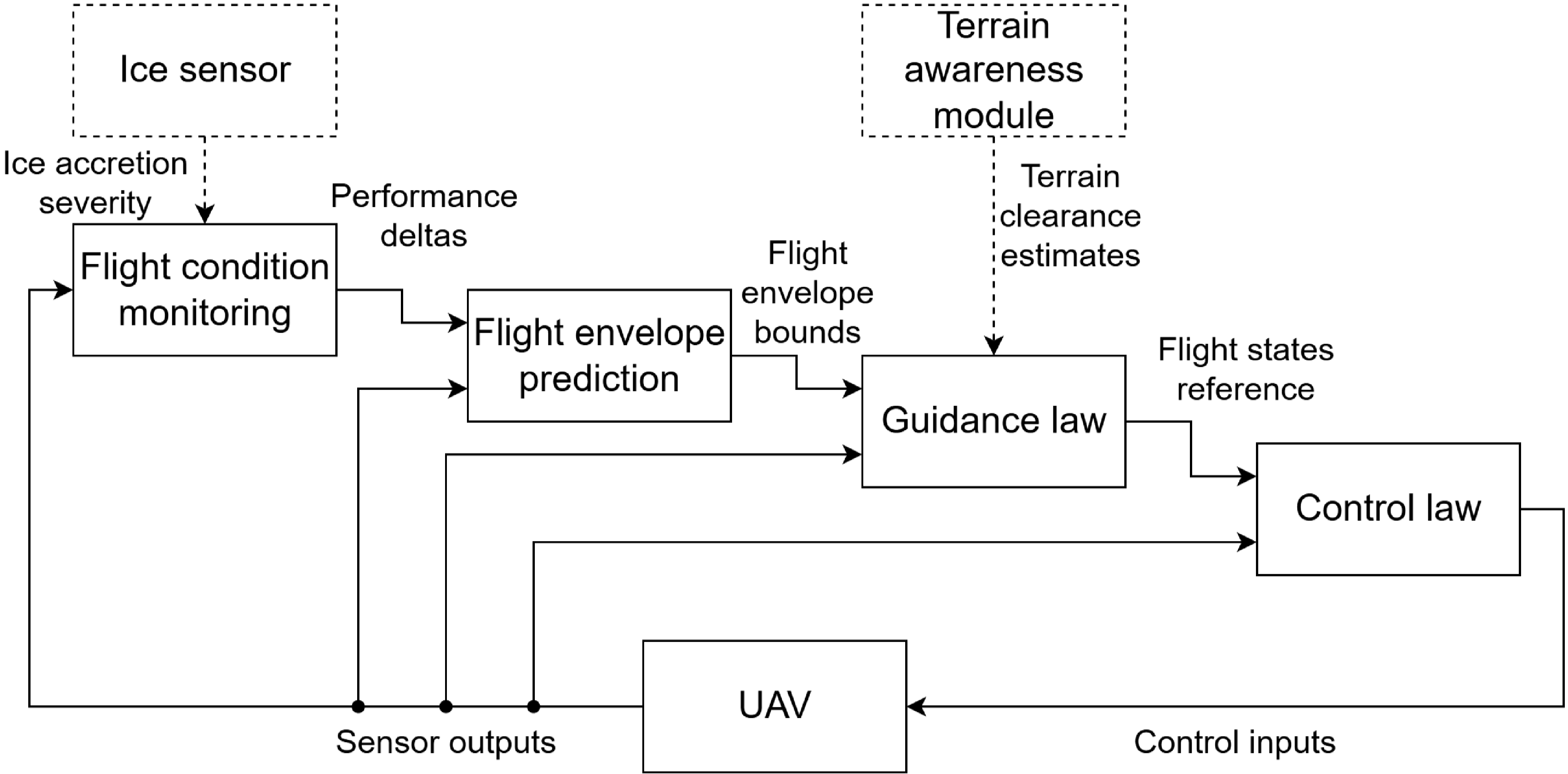







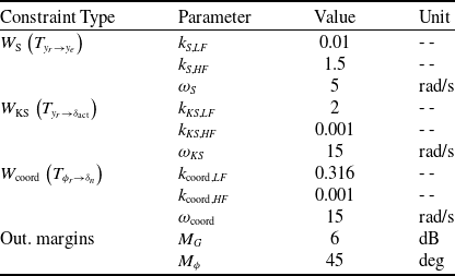

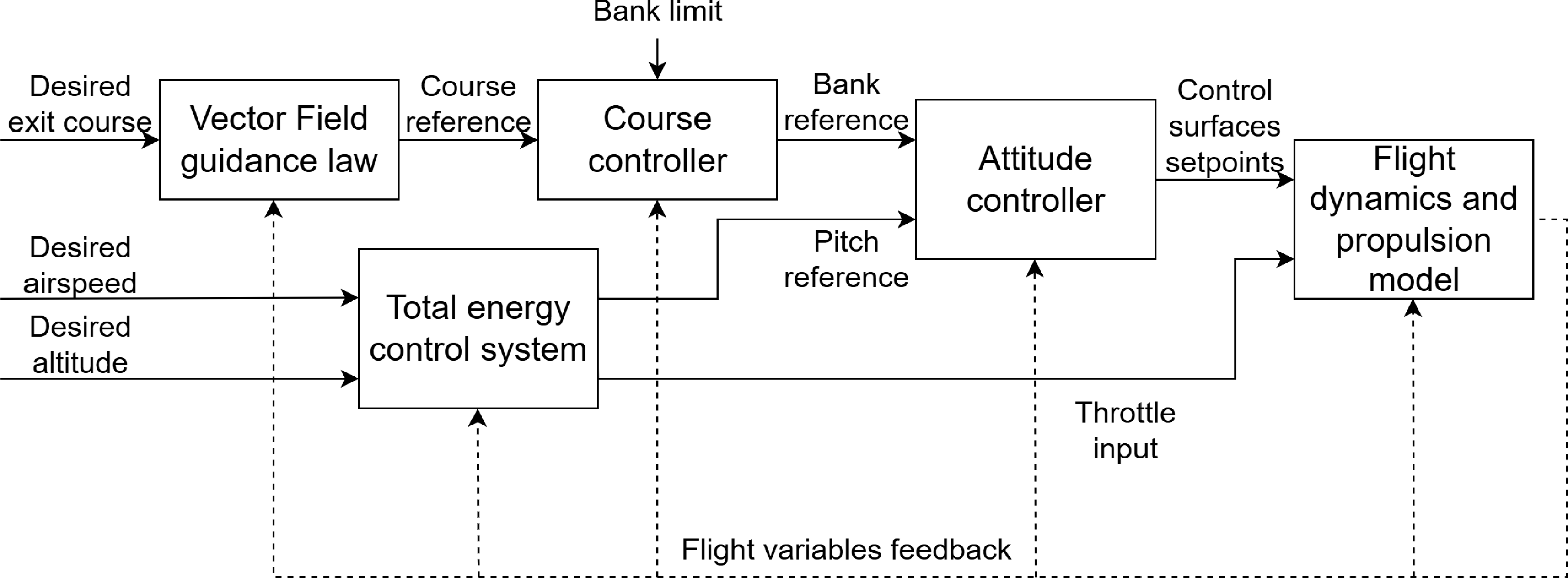
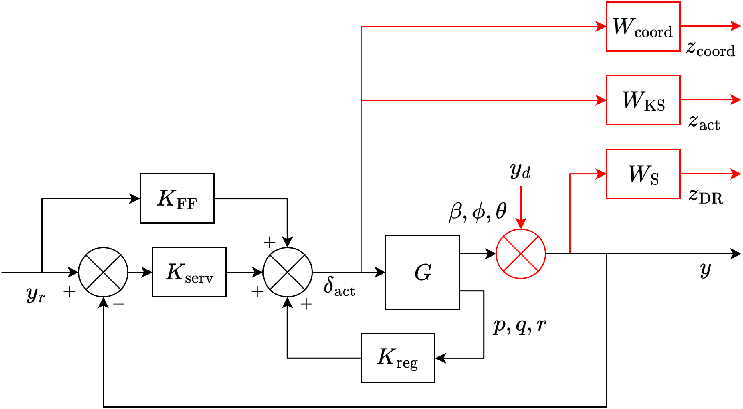
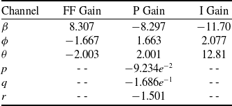


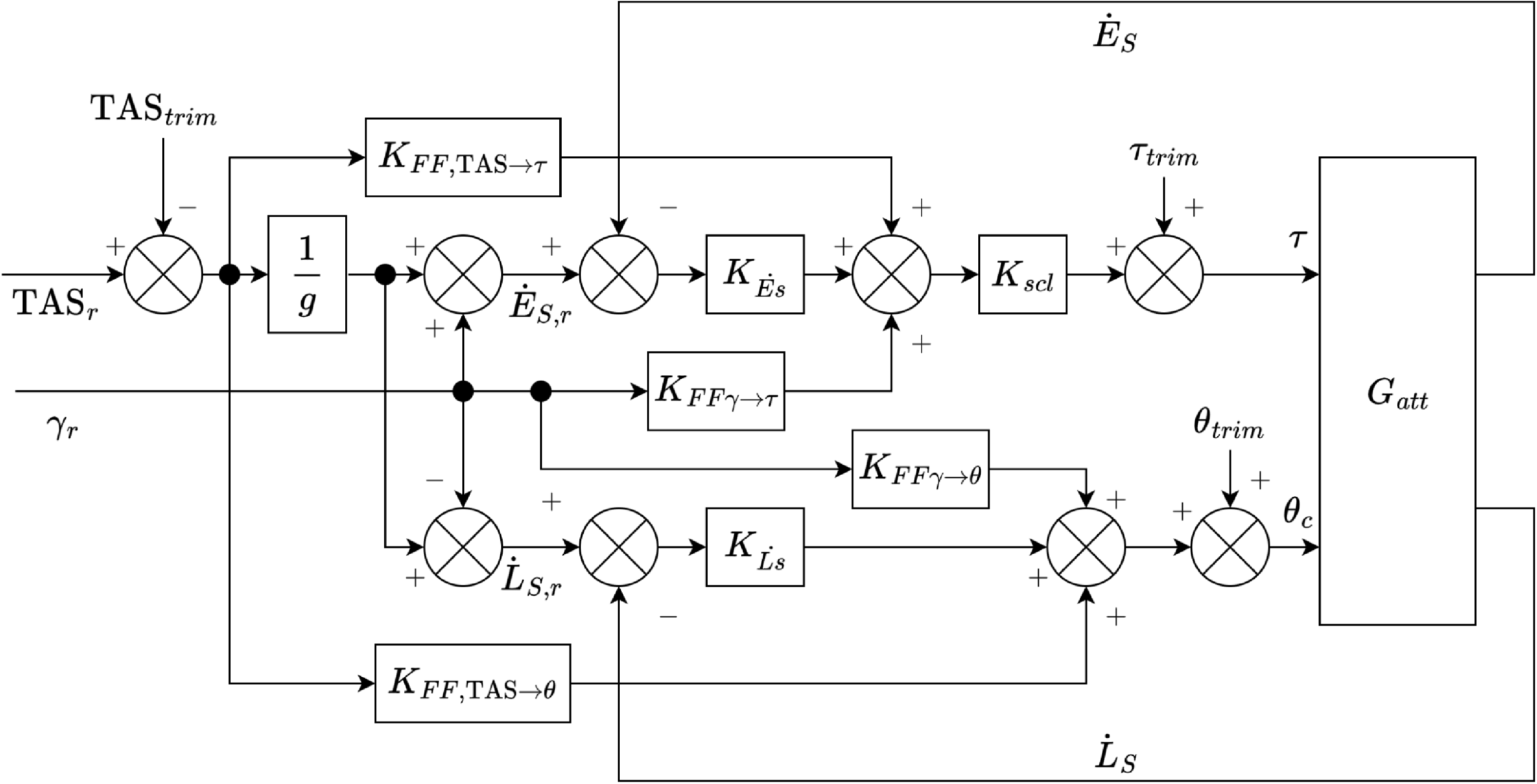
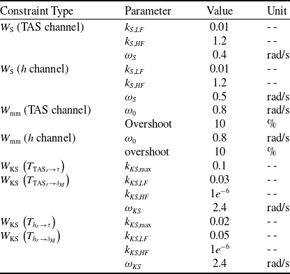
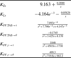


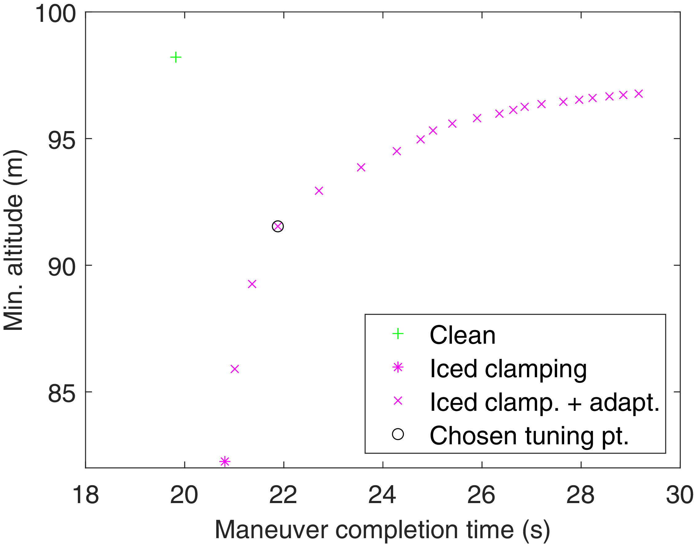
 hmin
 tmvr
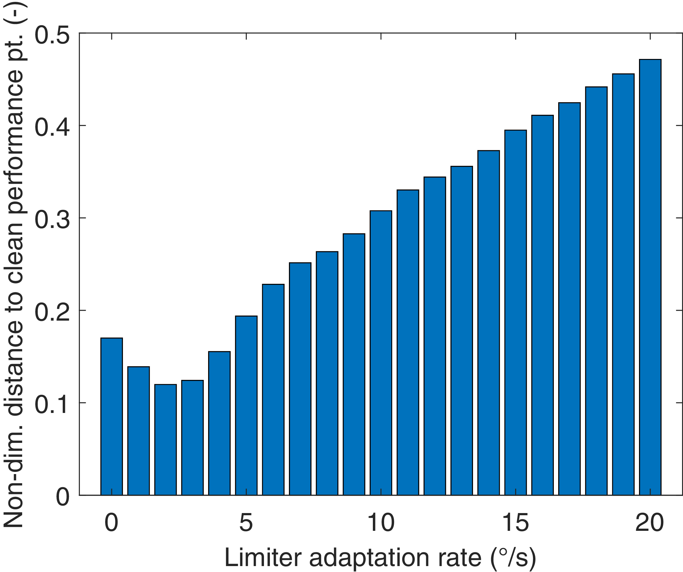
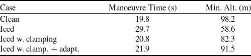

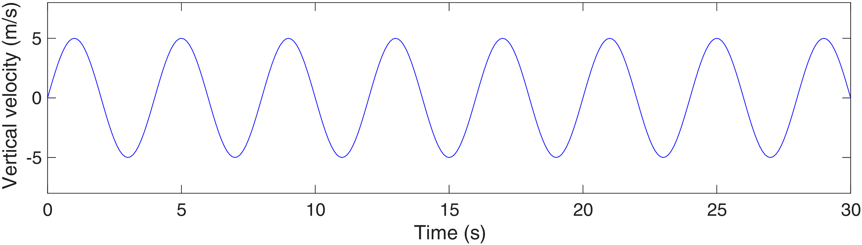

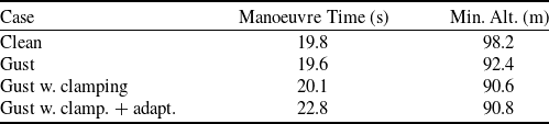

 Open access

