1 Introduction
Oscillatory wall-bounded flows (i.e. Stokes flows) are generally classified as either pulsatile, when the flow rate oscillates in time around a non-zero mean, or purely oscillatory (or reciprocating), when the cycle-averaged flow rate is zero (Di Liberto & Ciofalo Reference Di Liberto and Ciofalo2011). Oscillatory channel flow (OCF) is a wall-bounded unsteady flow that oscillates at a fixed angular frequency
 $\unicode[STIX]{x1D714}$
with a cycle-averaged zero mean velocity (for compactness we have omitted the descriptor ‘purely’). The cross-sectional mean flow over a half-period first accelerates to maximum velocity, next decelerates to zero velocity, then reverses direction. The process is then repeated indefinitely. The flow at a fixed point in space may either lead or lag the cross-sectional mean flow depending on wall-normal position and flow forcing. The dynamically important similarity variables are the Womersley number
 $\unicode[STIX]{x1D6FC}=h\sqrt{\unicode[STIX]{x1D714}/\unicode[STIX]{x1D708}}$
, where
 $h$
is the channel half-height,
 $\unicode[STIX]{x1D714}=2\unicode[STIX]{x03C0}/T$
with
 $T$
the period of oscillation, and
 $\unicode[STIX]{x1D708}$
is the fluid kinematic viscosity; and the peak Reynolds number
 $Re_{p}=2U_{m}h/\unicode[STIX]{x1D708}$
, where
 $U_{m}$
is the maximum amplitude of the cross-sectional mean velocity over a half-period. The square of the Womersley number,
 $\unicode[STIX]{x1D6FC}^{2}$
, characterizes the ratio of the diffusion time scale
 $h^{2}/\unicode[STIX]{x1D708}$
to the oscillation time scale
 $\unicode[STIX]{x1D714}^{-1}$
. The ratio
 $Re_{p}/\unicode[STIX]{x1D6FC}=\sqrt{2}Re_{s}$
, where
 $Re_{s}=U_{m}l_{s}/\unicode[STIX]{x1D708}$
is the Stokes Reynolds number and
 $l_{s}=\sqrt{2\unicode[STIX]{x1D708}/\unicode[STIX]{x1D714}}$
is the Stokes length.
Owing to its inherent unsteadiness, oscillatory wall-bounded flows exhibit complex dynamical behaviours relative to steady wall-bounded flow (Akhavan, Kamm & Shapiro Reference Akhavan, Kamm and Shapiro1991a ). In particular, in many engineering and environmental oscillatory flows, the flow is turbulent during part of the oscillation cycle and weakly transitional during the remaining part of the cycle. Since the fluid transport of mass, momentum and energy is profoundly different between weakly transitional and turbulent flow, it is of practical importance to study and understand transition to turbulence in oscillatory flow for prediction and control purposes. In the present study, direct numerical simulation (DNS) of oscillatory flow in a plane channel is used to gain an improved understanding of the evolution of the mean flow dynamics through transition with the aim to provide a mechanistic description of transition to turbulence in oscillatory wall-bounded flows.
1.1 Critical
 $Re_{s}$
of flow regime transitions

Experimental studies investigating transition to turbulence in oscillatory flows include Miller & Fejer (Reference Miller and Fejer1964), Sergeev (Reference Sergeev1966), Hino, Sawamoto & Takasu (Reference Hino, Sawamoto and Takasu1976), Akhavan et al. (Reference Akhavan, Kamm and Shapiro1991a
), Eckmann & Grotberg (Reference Eckmann and Grotberg1991) and Schmirler et al. (Reference Schmirler, Matěcha, Netřebská, Ježek and Adamec2014). Similarly, numerical simulations include Spalart & Baldwin (Reference Spalart and Baldwin1989), Akhavan, Kamm & Shapiro (Reference Akhavan, Kamm and Shapiro1991b
), Scotti & Piomelli (Reference Scotti and Piomelli2001), Di Liberto & Ciofalo (Reference Di Liberto and Ciofalo2011) and Ozdemir, Hsu & Balachandar (Reference Ozdemir, Hsu and Balachandar2014). Collectively, these studies identified five different flow regimes based on
 $Re_{s}$
: (I) laminar, (II) disturbed laminar, (III) self-sustaining transition, (IV) intermittently turbulent, (V) fully developed turbulent. A brief description of the generally accepted transition mechanism between different flow regimes, and the corresponding empirically determined critical value of
 $Re_{s}$
, denoted here by
 $Re_{s,a\rightarrow b}$
, where
 $a,b$
denote the flow regimes from which the flow transitions from and to, respectively, is provided below.
(i)
$Re_{s,I\rightarrow II}\approx 100$
(Hino et al.
Reference Hino, Sawamoto and Takasu1976; Akhavan et al.
Reference Akhavan, Kamm and Shapiro1991a
; Ozdemir et al.
Reference Ozdemir, Hsu and Balachandar2014): this transition is from a laminar flow (I) to a disturbed laminar flow (II). A disturbed laminar flow shows fluctuations in the instantaneous velocity, however, the mean velocity profile does not depart from the laminar profile. The transition mechanism is believed to be due to infinitesimally small disturbances that grow linearly to finite amplitude.(ii)
$Re_{s,II\rightarrow III}\approx 500$
(Hino et al.
Reference Hino, Sawamoto and Takasu1976; Akhavan et al.
Reference Akhavan, Kamm and Shapiro1991a
; Ozdemir et al.
Reference Ozdemir, Hsu and Balachandar2014): this transition is from a disturbed laminar flow (II) to a self-sustaining transitional flow (III). In a self-sustaining transitional flow, the mean velocity profiles depart from the laminar flow profile. The transition mechanism is believed to be due to finite-amplitude disturbances that grow nonlinearly and sustain unsteady fluctuations from one cycle to the next. The energy of the velocity fluctuations is, however, insufficient to trigger transition to a turbulent flow. Flow regime III was first proposed by Spalart & Baldwin (Reference Spalart and Baldwin1989) and has been extensively studied by Ozdemir et al. (Reference Ozdemir, Hsu and Balachandar2014).(iii)
$Re_{s,III\rightarrow IV}\approx 750$
(Ozdemir et al.
Reference Ozdemir, Hsu and Balachandar2014): in an intermittently turbulent flow, fully developed turbulent flow characteristics are first observed during the early decelerating phases of the cycle, while in the early accelerating phases of the cycle, turbulence is damped and the flow degenerates towards a weakly transitional flow. The underlying transition mechanism is believed to be due to a secondary instability mechanism of two-dimensional finite-amplitude waves to three-dimensional infinitesimal disturbances (Akhavan et al.
Reference Akhavan, Kamm and Shapiro1991b
; Ozdemir et al.
Reference Ozdemir, Hsu and Balachandar2014).(iv)
$Re_{s,IV\rightarrow V}\approx 3460$
(Jensen, Sumer & Fredsøe Reference Jensen, Sumer and Fredsøe1989): this transition is from an intermittently turbulent flow (IV) to a fully developed turbulent flow (V). In a fully developed turbulent flow, the flow exhibits fully developed turbulent flow characteristics over the entire cycle and a logarithmic mean velocity profile is absent for only 10 % of the oscillation period around the phase corresponding to flow reversal.


1.2 Transition to turbulence in oscillatory flow
The study of transition to turbulence in OCF is tantamount to studying transition from a type III to a type IV flow. The transition mechanism is generally accepted to be due to the local instability of the Stokes layer. However, owing to both the spatial and temporal variation of the flow, theoretical stability analysis of the Stokes layer is difficult and results of such analyses are not in agreement with experimental observations (Akhavan et al.
Reference Akhavan, Kamm and Shapiro1991a
; Ozdemir et al.
Reference Ozdemir, Hsu and Balachandar2014). To study this type of transition, Akhavan et al. (Reference Akhavan, Kamm and Shapiro1991b
) and Ozdemir et al. (Reference Ozdemir, Hsu and Balachandar2014) employed DNS to investigate the instability most likely to be responsible for transition. In these studies, a base laminar flow was perturbed by an initial prescribed disturbance and the evolution of the disturbance was tracked. By varying the prescribed initial disturbance, the type of instability most likely responsible for transition to turbulence can be identified. Akhavan et al. (Reference Akhavan, Kamm and Shapiro1991b
) reported that transition to turbulence in wall-bounded oscillatory flow likely results from a broadband secondary instability resulting from two-dimensional finite amplitude waves in the presence of three-dimensional infinitesimal disturbances. The two-dimensional finite-amplitude wave serves as an energy conduit between the mean flow and the three-dimensional disturbances and, given the right conditions, leads to exponential growth of the disturbance. Their simulation results showed that the three-dimensional disturbances decay to small but finite levels of energy during the early accelerating phases of the cycle but explosively grow prior to the start of the decelerating portion of the cycle. Ozdemir et al. (Reference Ozdemir, Hsu and Balachandar2014) reported that at
 $Re_{s}\approx 500$
linear instability leads to the formation of two-dimensional spanwise roller structures during the decelerating portion of the cycle. With increasing
 $Re_{s}$
nonlinear instabilities deform the roller structures into three-dimensional structures and the energy of the disturbances grows in amplitude. For
 $Re_{s}\approx 700$
, the energy of the three-dimensional disturbances is sufficiently large such that they are sustained from one cycle to the next and grow explosively during the late part of the accelerating portion of the cycle leading to transition to turbulence during the early part of the decelerating portion of the cycle. With increasing
 $Re_{s}$
, the duration of fully developed turbulence is observed to increase.
The objective of the present study is to gain an improved understanding of the differences in the mean flow dynamics between a self-sustaining transitional flow (type III) and an intermittently turbulent flow (type IV). The primary focus is to examine the differences in the mean flow dynamics in the part of the cycle where transition to turbulence occurs for the intermittently turbulent flows. The aim is to develop a mechanistic description of the transition to turbulence in OCF. This is achieved by analysing DNS datasets of OCF computed for
 $Re_{s}=648$
, 801 and 1009, representing type III and IV flow regimes. First, mean flow characteristics are analysed to highlight differences between the two flow regimes and to identify the regions of the cycle for
 $Re_{s}=801$
and 1009 that demark the transition region and the fully developed turbulent region. Next, the evolution of the mean flow dynamics over a period of oscillation is investigated to identify dynamical conditions important to the transition to turbulence. Further insights regarding the mean flow dynamics in OCF are gained by examining the evolution of the spectral characteristics associated with the Reynolds stress divergence. The present work is complementary to the studies of Akhavan et al. (Reference Akhavan, Kamm and Shapiro1991a
,Reference Akhavan, Kamm and Shapiro
b
) and Ozdemir et al. (Reference Ozdemir, Hsu and Balachandar2014).
2 Direct numerical simulation of oscillatory channel flow
The simulations employ a Cartesian domain defined by the orthonormal vector base
 $(\boldsymbol{e}_{x},\boldsymbol{e}_{y},\boldsymbol{e}_{z})=(\boldsymbol{e}_{1},\boldsymbol{e}_{2},\boldsymbol{e}_{3})$
where boldface denotes a vector, and
 $x$
,
 $y$
and
 $z$
are the streamwise, wall-normal and spanwise directions, respectively. The components of the velocity vector
 $u_{i}=\boldsymbol{u}$
are
 $u$
,
 $v$
and
 $w$
in the
 $x$
,
 $y$
and
 $z$
directions, respectively. The flow is incompressible,
 $$\begin{eqnarray}\frac{\unicode[STIX]{x2202}u_{i}}{\unicode[STIX]{x2202}x_{i}}=0,\end{eqnarray}$$
and driven by a cosinusoidal pressure gradient of amplitude
 $P_{0}$
at a prescribed frequency
 $\unicode[STIX]{x1D714}$
, given by the last term on the right-hand side of the following momentum transport equation:
 $$\begin{eqnarray}\frac{\unicode[STIX]{x2202}u_{i}}{\unicode[STIX]{x2202}t}+u_{j}\frac{\unicode[STIX]{x2202}u_{i}}{\unicode[STIX]{x2202}x_{j}}=-\frac{1}{\unicode[STIX]{x1D70C}}\frac{\text{d}p}{\text{d}x_{i}}+\unicode[STIX]{x1D708}\frac{\unicode[STIX]{x2202}^{2}u_{i}}{\unicode[STIX]{x2202}x_{j}^{2}}+\frac{1}{\unicode[STIX]{x1D70C}}P_{0}\cos (\unicode[STIX]{x1D714}t)\unicode[STIX]{x1D6FF}_{i1},\end{eqnarray}$$
where
 $\unicode[STIX]{x1D70C}$
is the fluid density,
 $p$
is pressure and
 $\unicode[STIX]{x1D6FF}_{ij}$
is the Kronecker delta. The computational domain is periodic in the streamwise and spanwise directions. The wall boundary conditions are no slip and no penetration. The design of the forcing term yields a net-zero flow rate over a full period.
Simulations were performed at
 $Re_{s}=648$
(
 $T=30,\unicode[STIX]{x1D6FC}=20.5$
),
 $Re_{s}=801$
(
 $T=30,\unicode[STIX]{x1D6FC}=25.1$
) and
 $Re_{s}=1009$
(
 $T=40,\unicode[STIX]{x1D6FC}=17.7$
). These values were chosen since the lowest
 $Re_{s}$
should correspond to a self-sustaining transitional flow (type III), the intermediate
 $Re_{s}$
should have just transitioned to an intermittently turbulent flow (type IV) and the highest
 $Re_{s}$
should be well within the intermittently turbulent flow regime. The computational domain size is
 $L_{x}=10h$
,
 $L_{y}=2h$
and
 $L_{z}=5h$
, which is identical to that used by Di Liberto & Ciofalo (Reference Di Liberto and Ciofalo2011) although the present resolution is higher with most simulations using
 $256^{3}$
cells. For
 $Re_{s}=648$
and
 $Re_{s}=1009$
grid independence studies were performed for three grids
 $64^{3}$
,
 $128^{3}$
,
 $256^{3}$
and
 $128^{3}$
,
 $256^{3}$
,
 $384^{3}$
, respectively. The two finest grids demonstrated statistical convergence while the coarsest grid showed a phase lag in
 $u_{\unicode[STIX]{x1D70F}}$
compared to the finer grids.
The DNS code is a well-validated finite difference code using non-dissipative second-order schemes for spatial derivatives on staggered grids (Dubief et al.
Reference Dubief, Terrapon, White, Shaqfeh, Moin and Lele2005). The fractional step method enforces incompressibility. The time advancement is third-order Runge–Kutta for the advection terms in all directions and the diffusive terms in the streamwise and spanwise directions. To relax the viscous stability constraint, the wall-normal diffusive term is advanced with a second-order Crank–Nicolson scheme. All simulations are performed with a dynamic time step which satisfies the Courant–Friedrichs–Lewy condition,
 $\unicode[STIX]{x0394}tu_{i}/\unicode[STIX]{x0394}x_{i}\leqslant 0.9$
, and a viscous stability condition,
 $\unicode[STIX]{x1D708}\unicode[STIX]{x0394}t/\min (\unicode[STIX]{x0394}x,\unicode[STIX]{x0394}y)<0.2$
. Both conditions are satisfied well below their maximum values for the numerical methods used here.
The flow is initialized with random white noise superimposed on the laminar flow field. A perturbation is then introduced over a short duration relative to the period of oscillation, in the form of periodic-in-space blowing and suction imposed through the wall boundary condition of the wall-normal velocity
 $$\begin{eqnarray}v(x,y=\pm h,z,t)={\mathcal{H}}(t)\left[A\sin \left(\frac{4\unicode[STIX]{x03C0}x}{L_{x}}\right)\cos \left(\frac{4\unicode[STIX]{x03C0}x}{L_{z}}\right)+\unicode[STIX]{x1D716}(t)\right],\end{eqnarray}$$
where
 ${\mathcal{H}}$
is a smooth step function, the amplitude
 $A=1u_{\unicode[STIX]{x1D70F},0}$
and
 $\unicode[STIX]{x1D716}(t)$
is random noise with a root mean square (r.m.s.) of
 $0.1u_{\unicode[STIX]{x1D70F},0}$
. The velocity
 $u_{\unicode[STIX]{x1D70F},0}=\sqrt{\unicode[STIX]{x1D70F}_{w}/\unicode[STIX]{x1D70C}}$
corresponds to the friction velocity for channel flow driven by a constant forcing term
 $P_{0}$
, where
 $\unicode[STIX]{x1D70F}_{w}$
is the wall shear stress. The initial transient decays after 2–4 cycles depending on
 $Re_{s}$
. The statistics described in the present paper are phase averaged over 10 periods after the initial transient decays. A period is divided into 32 phases for
 $Re_{s}=648$
and
 $Re_{s}=1009$
:
 $1\unicode[STIX]{x03C0}/16\leqslant \unicode[STIX]{x1D719}\leqslant 32\unicode[STIX]{x03C0}/16$
, where
 $\unicode[STIX]{x1D719}$
denotes the phase angle. Since
 $Re_{s}=801$
is near the transition Reynolds number, the phase sampling is increased and a period is divided into 48 phases. Because of this difference in the phase sampling, the
 $Re_{s}=801$
profiles are presented every other phase when all three
 $Re_{s}$
are plotted in the same figure. Note that omitted profiles in the data presentation for
 $Re_{s}=801$
trend the same as for the profiles that are shown every other phase. For ease of interpretation, and when appropriate, data are presented only for a half-cycle (owing to anti-symmetry) and separated between the accelerating phases and decelerating phases of the cycle. Simulations performed when dividing a period into 128 phases (not shown) showed a slight phase shift and amplitude modulation for some statistics compared to the statistics acquired for a lower number of phases. This is attributable to a smaller averaging duration. One challenge with the higher phase sampling is statistical convergence, in particular during the phases when the Reynolds stress grows explosively.
(a) The wall shear stress
 $\unicode[STIX]{x1D70F}_{w}$
, normalized by
 $l_{s}P_{0}/\sqrt{2}$
and (b) the skin friction coefficient
 $C_{f}=2\unicode[STIX]{x1D70F}_{w}/\unicode[STIX]{x1D70C}U_{c}^{2}$
normalized by
 $\sqrt{2}\unicode[STIX]{x1D70C}l_{s}\unicode[STIX]{x1D714}^{2}/P_{0}$
, where
 $U_{c}$
is the centreline velocity, plotted as a function of
 $\unicode[STIX]{x1D719}$
for
 $Re_{s}=648$


3 Results
3.1 Mean flow behaviours
The wall shear stress,
 $\unicode[STIX]{x1D70F}_{w}$
, normalized by
 $l_{s}P_{0}/\sqrt{2}$
and the skin friction coefficient
 $C_{f}=2\unicode[STIX]{x1D70F}_{w}/\unicode[STIX]{x1D70C}U_{c}^{2}$
normalized by
 $\sqrt{2}\unicode[STIX]{x1D70C}l_{s}\unicode[STIX]{x1D714}^{2}/P_{0}$
, where
 $U_{c}$
is the centreline velocity, are plotted as a function of
 $\unicode[STIX]{x1D719}$
in figures 1(a) and 1(b), respectively, for the three
 $Re_{s}$
. With these normalizations,
 $\unicode[STIX]{x1D70F}_{w}$
and
 $C_{f}$
for the laminar flow case are invariant to
 $\unicode[STIX]{x1D6FC}$
. The wall shear stress analytically computed for laminar oscillatory channel flow is shown as a line with circular symbols in each figure. Figure 1(a) shows that the wall shear stress profiles for the three
 $Re_{s}$
nearly collapse on the laminar profile during the early accelerating phases (
 $1\unicode[STIX]{x03C0}/16\lesssim \unicode[STIX]{x1D719}\lesssim \unicode[STIX]{x03C0}/4$
) and collapse on each other (but not the laminar curve) during the late decelerating phases (
 $13\unicode[STIX]{x03C0}/16\lesssim \unicode[STIX]{x1D719}\lesssim \unicode[STIX]{x03C0}$
) of the first half-period. (Owing to anti-symmetry, the second half-period shows identical results.) The deviation from the laminar curve for both higher
 $Re_{s}$
occurs at
 $\unicode[STIX]{x1D719}\approx \unicode[STIX]{x03C0}/4$
(although the slope of the two profiles are quite different at this point), while the wall shear stress at
 $Re_{s}=648$
first deviates from the laminar curve later in the cycle at
 $\unicode[STIX]{x1D719}\approx \unicode[STIX]{x03C0}/2$
.
The
 $C_{f}$
profiles in figure 1(b) show that the profiles for
 $Re_{s}=1009$
and
 $Re_{s}=801$
discernibly break from the laminar curve at
 $\unicode[STIX]{x1D719}\approx 6\unicode[STIX]{x03C0}/16$
and
 $\unicode[STIX]{x1D719}\approx 7\unicode[STIX]{x03C0}/16$
, respectively. The two profiles then rapidly increase with different slopes up to their maximum value after which they decrease approximately linearly with the same slope until
 $\unicode[STIX]{x1D719}\approx 3\unicode[STIX]{x03C0}/4$
. With increasing
 $\unicode[STIX]{x1D719}$
the two now collapsed profiles decrease until
 $\unicode[STIX]{x1D719}\approx 14\unicode[STIX]{x03C0}/16$
. These behaviours are significant on a number of accounts. The point of departure of
 $C_{f}$
from the laminar curve until it reaches its maximum value demarks the transition region. The rapid rise in
 $C_{f}$
within the transition region demarks the nonlinear development stage. With increasing
 $Re_{s}$
, the nonlinear development stage occurs earlier in the cycle and the growth of
 $C_{f}$
is more explosive (i.e. occurs over a shorter
 $\unicode[STIX]{x0394}\unicode[STIX]{x1D719}$
). The approximately linear decay in
 $C_{f}$
in the early part of the decelerating portion of the cycle is reminiscent of the behaviour of
 $C_{f}$
in fully developed turbulent channel flow with increasing
 $Re_{\unicode[STIX]{x1D703}}$
(Wu & Moin Reference Wu and Moin2010). The point of departure from the laminar curve for
 $Re_{s}=648$
occurs at
 $\unicode[STIX]{x1D719}\approx 9\unicode[STIX]{x03C0}/16$
, a rapid rise in
 $C_{f}$
is not observed, and its maximum value is lower than that for the higher
 $Re_{s}$
.
Phase-averaged profiles of mean streamwise velocity in wall units for
 $Re_{s}=648$

 $Re_{s}=801$

 $Re_{s}=1009$

 $Re_{\unicode[STIX]{x1D70F}}=1000$


Phase-averaged wall-normal profiles of the mean velocity for the three
 $Re_{s}$
as a function of
 $\unicode[STIX]{x1D719}$
is given in figure 2. Profiles for
 $Re_{s}=801$
are shown every other phase so that the data for the three
 $Re_{s}$
can be presented in the same plot. The superscript
 $^{+}$
denotes normalization by the friction velocity
 $u_{\unicode[STIX]{x1D70F}}$
and kinematic viscosity
 $\unicode[STIX]{x1D708}$
. Profiles from steady turbulent channel flow from the Johns Hopkins Turbulence Databases (JHTDB) at
 $Re_{\unicode[STIX]{x1D70F}}=1000$
are shown for baseline comparison. As is apparent from the phase evolution of the mean velocity profiles, the
 $Re_{s}=648$
profiles differ significantly from the steady turbulent channel flow profiles throughout the cycle. The
 $Re_{s}=1009$
profiles fall close to the steady turbulent channel flow profiles starting from the end of the accelerating portion of the cycle through the first half of the decelerating portion of the cycle. Similarly, the profiles for
 $Re_{s}=801$
fall close to the steady turbulent channel flow profiles during the first half of the decelerating portion of the cycle.
The two higher
 $Re_{s}$
show an apparent logarithmic dependence of the wall-normal mean velocity distribution in an interior region of flow during the early decelerating portion of the cycle of the form
 $$\begin{eqnarray}\langle u\rangle ^{+}=\frac{1}{\unicode[STIX]{x1D705}}\ln (y^{+})+B,\end{eqnarray}$$
where
 $\langle \cdot \rangle$
denotes an average,
 $1/\unicode[STIX]{x1D705}$
(typically
 $\unicode[STIX]{x1D705}$
is called the von Kármán coefficient) is the slope and
 $B$
(i.e. the additive constant) is the intercept at
 $y^{+}=1$
. In steady turbulent wall-bounded flow, equation (3.1) is a dimensional necessity when the inner (
 $\unicode[STIX]{x1D6FF}_{\unicode[STIX]{x1D708}}=\unicode[STIX]{x1D708}/u_{\unicode[STIX]{x1D70F}}$
) and outer (
 $h$
) length scales are sufficiently separated, i.e. when
 $h^{+}$
is sufficiently large (Smits, McKeon & Marusic Reference Smits, McKeon and Marusic2011). In steady turbulent channel flow over hydraulically smooth walls
 $\unicode[STIX]{x1D705}\approx 0.4$
and
 $B\approx 5.2$
with some existing evidence for variations depending on the Reynolds number (Nagib & Chauhan Reference Nagib and Chauhan2008).
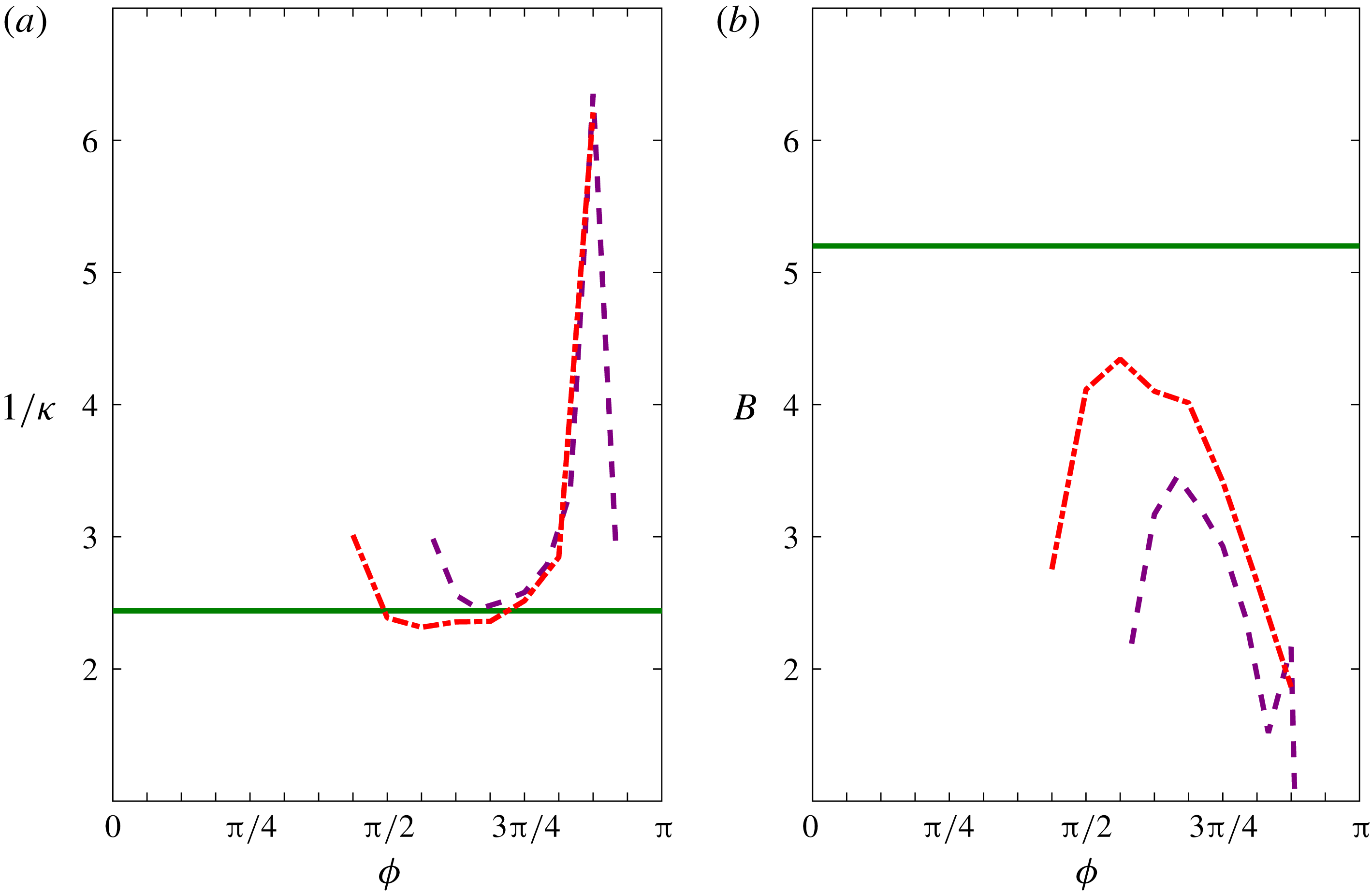
The value of the slope (
 $1/\unicode[STIX]{x1D705}$
) and the intercept (
 $B$
) of the logarithmic region of the mean velocity profiles in OCF at the two highest
 $Re_{s}$
are shown in figure 3, where the slope was determined from the so-called indicator function
 $[y^{+}(\text{d}\langle u\rangle ^{+}/\text{d}y^{+})]$
and the intercept was determined by curve fits to the mean velocity data within the logarithmic region using the slope determined from the indicator function. Observed in the figure is that for
 $Re_{s}=1009$
, once a logarithmic region emerges at
 $\unicode[STIX]{x1D719}\approx 7\unicode[STIX]{x03C0}/16$
, the slope rapidly attains the expected value of
 $1/\unicode[STIX]{x1D705}\approx 2.5$
for steady turbulent channel flow at low Reynolds number and remains at this value during the early decelerating portion of the cycle (
 $\unicode[STIX]{x03C0}/2\lesssim \unicode[STIX]{x1D719}\lesssim 11\unicode[STIX]{x03C0}/16$
). The slope then slowly increases with increasing phase until
 $\unicode[STIX]{x1D719}\approx 13\unicode[STIX]{x03C0}/16$
where the slope rapidly increases, after which the logarithmic region ceases to exist. For
 $Re_{s}=801$
, a logarithmic region emerges at
 $\unicode[STIX]{x1D719}\approx 9\unicode[STIX]{x03C0}/16$
and the slope is greater than
 $1/\unicode[STIX]{x1D705}\approx 2.5$
for all phases that show a logarithmic distribution of mean velocity. The intercept is shown to be a function of
 $Re_{s}$
and phase,
 $B(Re_{s},\unicode[STIX]{x1D719})$
, and always falls below the expected value of
 $B=5.2$
for steady turbulent channel flow.
Values of the (a) von Kármán coefficient
 $\unicode[STIX]{x1D705}$
and (b) the intercept
 $B$
as given by (3.1) for the phase angles in the cycle when a logarithmic dependence of the mean velocity profile is observed in OCF for the two higher
 $Re_{s}$
. The line styles are the same as in figure 2.

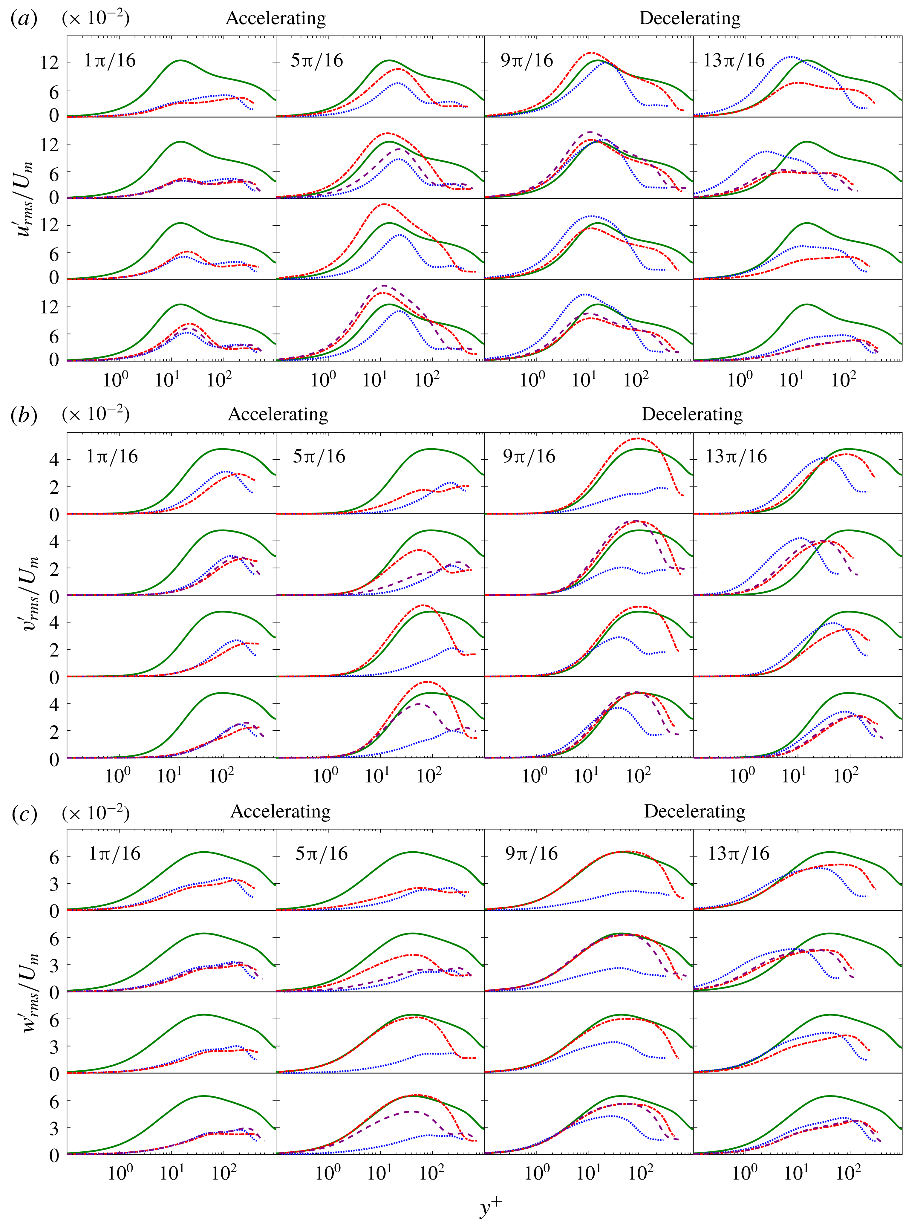
Phase-averaged profiles of the r.m.s. velocity fluctuations normalized by
 $U_{m}$
as a function of
 $\unicode[STIX]{x1D719}$
: (a)
 $u_{rms}^{\prime }$
, (b)
 $v_{rms}^{\prime }$
and (c)
 $w_{rms}^{\prime }$
. The line styles are the same as in figure 2.

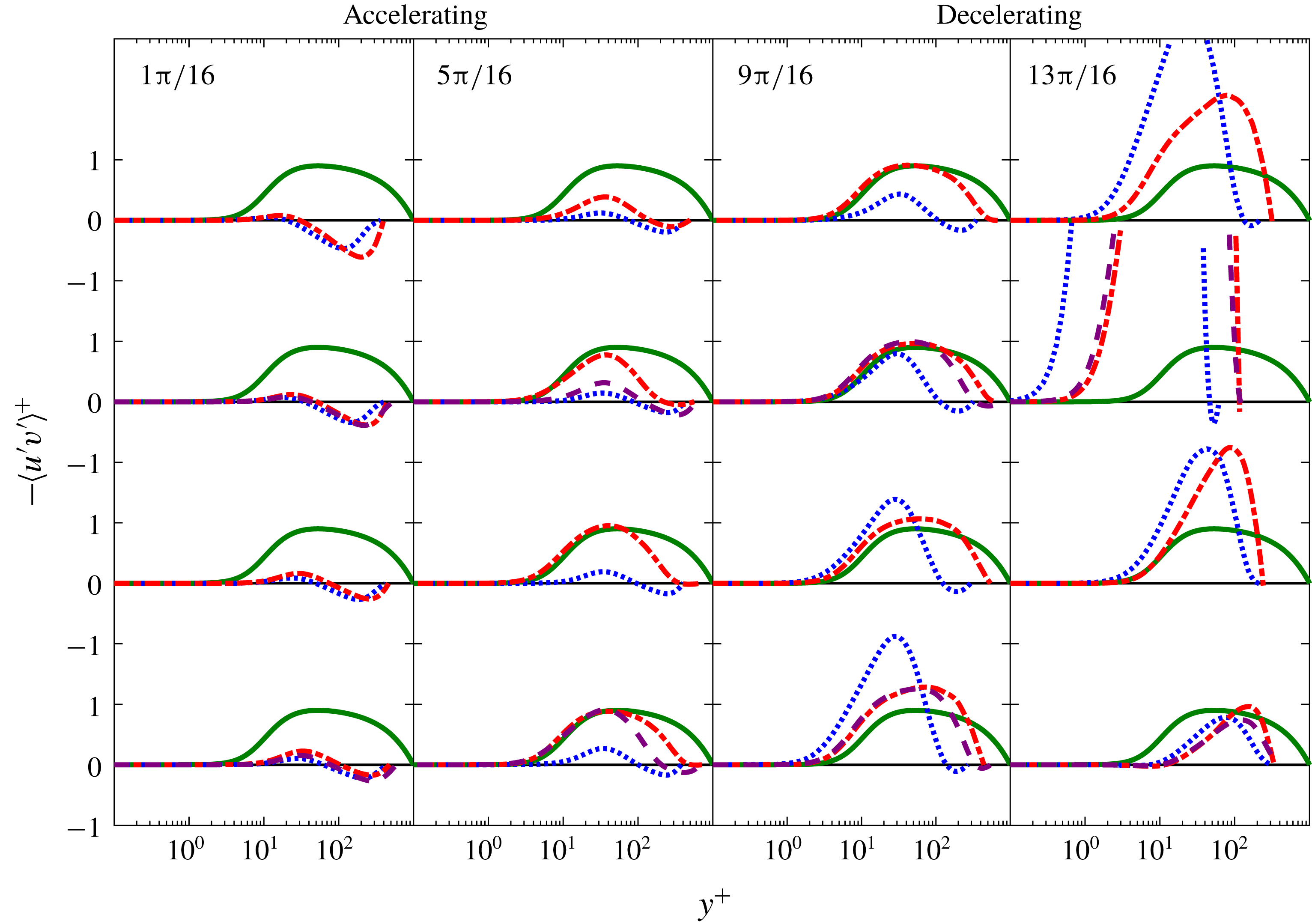
Phase-averaged profiles of the Reynolds stress in wall units as functions of
 $\unicode[STIX]{x1D719}$
. The line styles are the same as in figure 2.

Wall-normal profiles of the r.m.s. velocity fluctuations
 $u_{i,rms}^{\prime }=\langle u_{i}^{\prime 2}\rangle ^{1/2}$
are shown in figure 4 for the three
 $Re_{s}$
. The r.m.s. profiles are scaled by
 $U_{m}$
rather than
 $u_{\unicode[STIX]{x1D70F}}$
since the zero crossings of
 $u_{\unicode[STIX]{x1D70F}}$
proved problematic for both data presentation and interpretation. The streamwise r.m.s. fluctuations
 $u_{rms}^{\prime }$
are relatively small with a maximum in the outer layer at
 $y^{+}\approx 200$
at the starting phase of the accelerating portion of the cycle. With increasing
 $\unicode[STIX]{x1D719}$
, the r.m.s. fluctuations in the outer layer decrease and the peak r.m.s. fluctuations begin to form at
 $y^{+}\approx 25$
due to increasing levels of shear in the Stokes layer. At a phase angle consistent with the phase angle where
 $\unicode[STIX]{x1D70F}_{w}$
departs from the laminar curve, the peak location of
 $u_{rms}^{\prime }$
shifts to
 $y^{+}\approx 10$
. The peak then increases in magnitude and reaches a maximum at
 $\unicode[STIX]{x1D719}\approx 7\unicode[STIX]{x03C0}/16,8\unicode[STIX]{x03C0}/16,12\unicode[STIX]{x03C0}/16$
for
 $Re_{s}=1009,801,648$
, respectively. The
 $u_{rms}^{\prime }$
fluctuations then monotonically decrease with increasing
 $\unicode[STIX]{x1D719}$
returning to their initial values late in the decelerating portion of the cycle.
The r.m.s. fluctuations in the wall-normal
 $v_{rms}^{\prime }$
and spanwise directions
 $w_{rms}^{\prime }$
behave similarly to each other but exhibit different behaviours than the streamwise r.m.s. fluctuations. At the starting phase of the accelerating portion of the cycle,
 $v_{rms}^{\prime }$
and
 $w_{rms}^{\prime }$
are small near the wall and have a maximum at
 $100\lesssim y^{+}\lesssim 200$
, dependent on
 $Re_{s}$
. From
 $\unicode[STIX]{x03C0}/16\lesssim \unicode[STIX]{x1D719}\lesssim 5\unicode[STIX]{x03C0}/16$
, both
 $v_{rms}^{\prime }$
and
 $w_{rms}^{\prime }$
decrease for all
 $Re_{s}$
. Substantial increase in
 $v_{rms}^{\prime }$
and
 $w_{rms}^{\prime }$
in the near-wall region (i.e.
 $y^{+}<100$
) first occurs at
 $\unicode[STIX]{x1D719}\approx 6\unicode[STIX]{x03C0}/16,8\unicode[STIX]{x03C0}/16,11\unicode[STIX]{x03C0}/16$
and the peak reaches a maximum at
 $\unicode[STIX]{x1D719}\approx 9\unicode[STIX]{x03C0}/16,10\unicode[STIX]{x03C0}/16,14\unicode[STIX]{x03C0}/16$
for
 $Re_{s}=1009,801,648$
, respectively. The r.m.s. profiles for
 $Re_{s}=1009$
and
 $Re_{s}=801$
are similar to steady turbulent channel flow from
 $7\unicode[STIX]{x03C0}/16\lesssim \unicode[STIX]{x1D719}\lesssim 12\unicode[STIX]{x03C0}/16$
and
 $8\unicode[STIX]{x03C0}/16\lesssim \unicode[STIX]{x1D719}\lesssim 12\unicode[STIX]{x03C0}/16$
, respectively, although the r.m.s. fluctuations for OCF are smaller in the outer layer. The
 $u_{rms}^{\prime }$
profiles for
 $Re_{s}=648$
are most similar to steady turbulent channel flow from
 $9\unicode[STIX]{x03C0}/16\lesssim \unicode[STIX]{x1D719}\lesssim 12\unicode[STIX]{x03C0}/16$
in the near-wall region but the
 $v_{rms}^{\prime }$
and
 $w_{rms}^{\prime }$
profiles are substantially different than the steady turbulent channel profiles during these phase angles.
Phase-averaged wall-normal profiles of the Reynolds stress for the three
 $Re_{s}$
as a function of
 $\unicode[STIX]{x1D719}$
are given in figure 5. Here it is observed that a finite Reynolds stress exists at all phases of the cycle for the three
 $Re_{s}$
. This is perhaps surprising since, despite a finite Reynolds stress, the
 $C_{f}$
profiles for all three
 $Re_{s}$
fall approximately on the laminar profile during the early part of the accelerating portion of the cycle. The phase angle where the Reynolds stress rapidly increases for each
 $Re_{s}$
is nearly identical with the phase angle where
 $C_{f}$
departs from the laminar curve as described above. The
 $Re_{s}=1009$
profiles fall close to the steady turbulent channel flow profiles from
 $7\unicode[STIX]{x03C0}/16\lesssim \unicode[STIX]{x1D719}\lesssim 12\unicode[STIX]{x03C0}/16$
. The
 $Re_{s}=801$
profiles fall close to the steady turbulent channel flow profiles from
 $\unicode[STIX]{x03C0}/2\lesssim \unicode[STIX]{x1D719}\lesssim 11\unicode[STIX]{x03C0}/16$
. For
 $Re_{s}=648$
rapid growth of the Reynolds stress begins at
 $\unicode[STIX]{x1D719}\approx 9\unicode[STIX]{x03C0}/16$
but the Reynolds stress profiles remain distinctly different than the steady turbulent channel flow profiles for all phases of the cycle.
The mean flow characteristics presented in figures 1–5 clearly demonstrate that
 $Re_{s}=648$
is a self-sustaining transitional (type III) flow and
 $Re_{s}=801$
and
 $Re_{s}=1009$
are intermittently turbulent (type IV) flows, in agreement with
 $Re_{s,III\rightarrow IV}\approx 750$
. Specifically,
 $Re_{s}=1009$
and
 $Re_{s}=801$
exhibit turbulent characteristics similar to steady turbulent channel flow from
 $7\unicode[STIX]{x03C0}/16\lesssim \unicode[STIX]{x1D719}\lesssim 12\unicode[STIX]{x03C0}/16$
and
 $8\unicode[STIX]{x03C0}/16\lesssim \unicode[STIX]{x1D719}\lesssim 12\unicode[STIX]{x03C0}/16$
, respectively, and
 $Re_{s}=648$
does not show turbulent characteristics similar to steady turbulent channel flow during any part of the cycle. These figures also demonstrate the profound differences in the mean flow dynamics between type III and type IV flows. These difference will be explored in detail below.
3.2 Mean flow dynamics
The inner-normalized phase-averaged
 $x$
-momentum equation for an OCF is
 $$\begin{eqnarray}\underbrace{\frac{\text{d}\langle P\rangle ^{+}}{\text{d}x^{+}}}_{A^{\ast }}+\underbrace{\frac{\unicode[STIX]{x2202}^{2}\langle u\rangle ^{+}}{\unicode[STIX]{x2202}y^{+2}}}_{B^{\ast }}+\underbrace{\frac{\unicode[STIX]{x2202}\langle -u^{\prime }v^{\prime }\rangle ^{+}}{\unicode[STIX]{x2202}y^{+}}}_{C^{\ast }}\underbrace{-\frac{\unicode[STIX]{x2202}\langle u\rangle ^{+}}{\unicode[STIX]{x2202}t^{+}}}_{D^{\ast }}=0.\end{eqnarray}$$
From left-to-right in (3.2), term
 $A^{\ast }$
is the mean pressure gradient, term
 $B^{\ast }$
is the mean viscous force, term
 $C^{\ast }$
is the net mean effect of turbulent inertia and term
 $D^{\ast }$
is the unsteady term (herein called the local acceleration). To investigate the mechanism of transition to fully developed turbulence (from type III to IV), the phase evolution of the turbulent inertia (term
 $C^{\ast }$
) and the local acceleration (term
 $D^{\ast }$
) are examined. The former because it is an indicator of the emerging importance of turbulent transport and the latter because it captures the time evolution of the flow. Particular focus is on the late stages of the accelerating portion of the cycle corresponding to the transition region for
 $Re_{s}=801$
and
 $Re_{s}=1009$
as determined from figure 1 and supported by the mean flow statistics presented above.
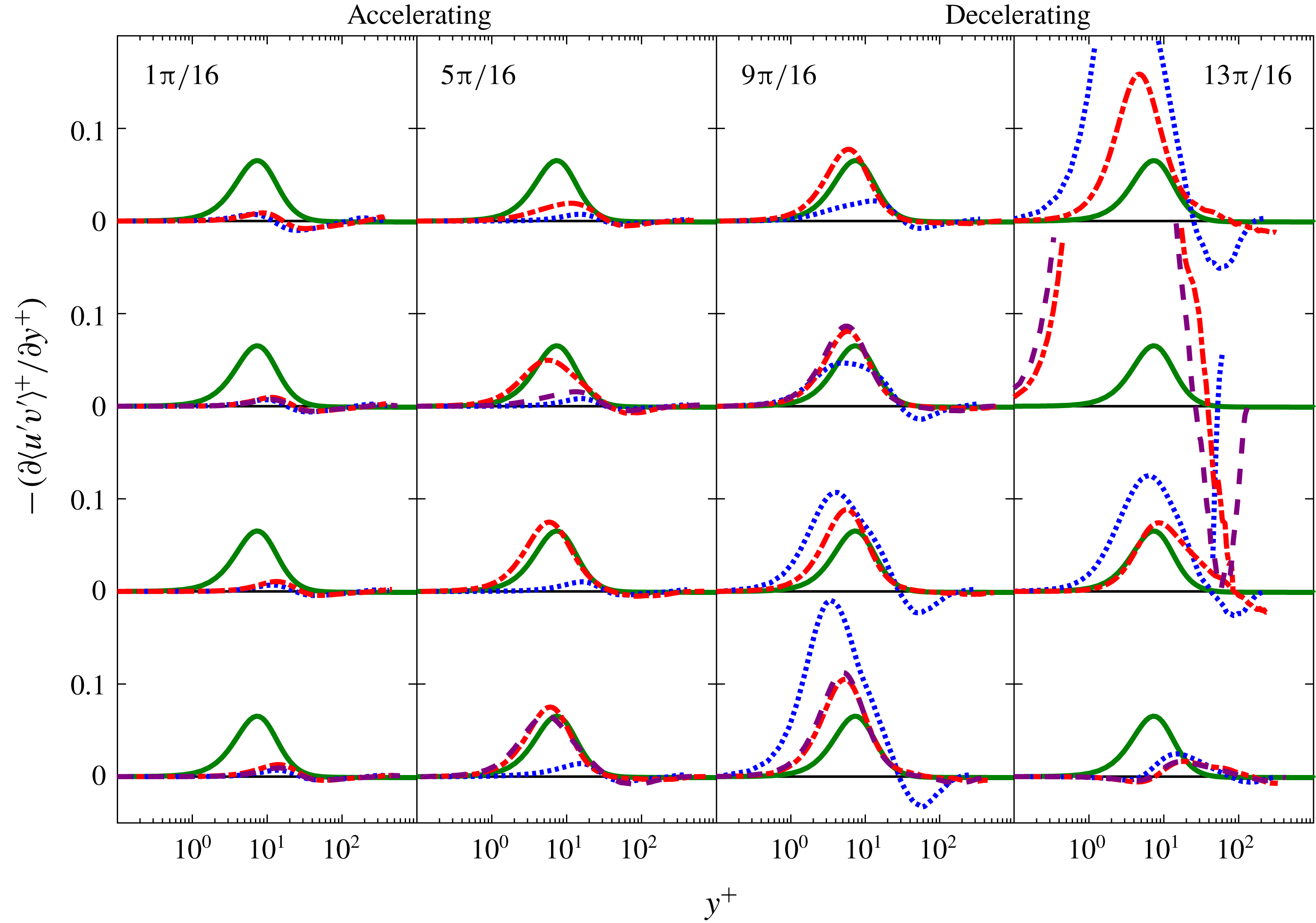
Phase-averaged profiles of the Reynolds stress gradient as a function of
 $\unicode[STIX]{x1D719}$
. The line styles are the same as in figure 2. The turbulent inertia profiles from
 $(13\unicode[STIX]{x03C0}/16)\leqslant \unicode[STIX]{x1D719}\leqslant (14\unicode[STIX]{x03C0}/16)$
have the same general shape as the profiles in the preceding phase angle but owing to the small magnitude of
 $\unicode[STIX]{x1D70F}_{w}$
do not fit within the limits of the figure.

3.3 Evolution of turbulent inertia
$(-\unicode[STIX]{x2202}\langle u^{\prime }v^{\prime }\rangle ^{+}/\unicode[STIX]{x2202}y^{+})$

The evolution of the turbulent inertia (term
 $C^{\ast }$
) plotted as a function of
 $\unicode[STIX]{x1D719}$
is shown in figure 6 for the three
 $Re_{s}$
. Profiles from steady turbulent channel flow from the JHTDB at
 $Re_{\unicode[STIX]{x1D70F}}=1000$
are shown for baseline comparison. It is observed that a finite Reynolds stress gradient (and consequently a finite Reynolds stress as shown previously) exists for all phases in the cycle for the three
 $Re_{s}$
. Rapid growth of turbulent inertia begins at
 $\unicode[STIX]{x1D719}\approx 5\unicode[STIX]{x03C0}/16$
and
 $\unicode[STIX]{x1D719}\approx 7\unicode[STIX]{x03C0}/16$
, for
 $Re_{s}=1009$
and
 $Re_{s}=801$
, respectively, and are nearly identical with the phase angle where
 $C_{f}$
departs from the laminar curve. The
 $Re_{s}=1009$
profiles fall close to the steady turbulent channel flow profiles from
 $7\unicode[STIX]{x03C0}/16\lesssim \unicode[STIX]{x1D719}\lesssim 9\unicode[STIX]{x03C0}/16$
and have a similar shape but larger magnitude than steady turbulent channel flow from
 $10\unicode[STIX]{x03C0}/16\lesssim \unicode[STIX]{x1D719}\lesssim 12\unicode[STIX]{x03C0}/16$
. Similarly, the
 $Re_{s}=801$
profiles fall close to the steady turbulent channel flow profiles from
 $8\unicode[STIX]{x03C0}/16\lesssim \unicode[STIX]{x1D719}\lesssim 9\unicode[STIX]{x03C0}/16$
and have a similar shape but larger magnitude than steady turbulent channel flow from
 $9\unicode[STIX]{x03C0}/16\lesssim \unicode[STIX]{x1D719}\lesssim 12\unicode[STIX]{x03C0}/16$
. For
 $Re_{s}=648$
, rapid growth of the turbulent inertia begins at
 $\unicode[STIX]{x1D719}\approx 10\unicode[STIX]{x03C0}/16$
but remains different from the steady turbulent channel flow profiles for all phases of the cycle.
When viewed as a force-like term in the mean momentum balance, the turbulent inertia is often categorized by its source-like and sink-like characteristics (Elsnab et al. Reference Elsnab, Klewicki, Maynes and Ameel2011) since
 $$\begin{eqnarray}\int _{0}^{h^{+}}\frac{\unicode[STIX]{x2202}\langle -uv\rangle ^{+}}{\unicode[STIX]{x2202}y^{+}}\,\text{d}y^{+}=0.\end{eqnarray}$$
Here positive (negative) regions of
 $\unicode[STIX]{x2202}\langle -u^{\prime }v^{\prime }\rangle ^{+}/\unicode[STIX]{x2202}y^{+}$
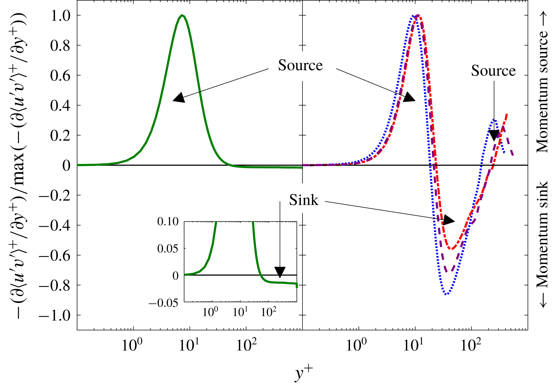
are associated with a source-like (sink-like) region. In steady turbulent channel flow (zero-pressure-gradient (ZPG) boundary layer flow as well) there is a single momentum source and a single momentum sink as illustrated in the left panel of figure 7. The momentum source, of large magnitude, is confined to a narrow region near the wall on the wallward side of the peak location of the Reynolds stress. While the momentum sink, of low magnitude, extends from above the location of peak Reynolds stress to the channel centreline (or edge of the boundary layer in ZPG flow). Consequently, on average, the action of turbulent inertia is to transport momentum from the outer layer (i.e. the sink region) to the inner layer (i.e. the source region) of the flow.
Normalized profiles of turbulent inertia for (left) fully developed channel flow (Perlman et al.
Reference Perlman, Burns, Li and Meneveau2007) and (right) OCF at
 $\unicode[STIX]{x1D719}=2\unicode[STIX]{x03C0}/16$
. The line styles are the same as in figure 2. In the left panel there is one positive region (momentum source) and one negative region (momentum sink). In the right panel there are two positive regions (i.e. two momentum sources) and one negative region (momentum sink).

Contribution of sink-like and source-like behaviours of the turbulent inertia for
 $Re_{s}=648$
(a),
 $Re_{s}=801$
(b) and
 $Re_{s}=1009$
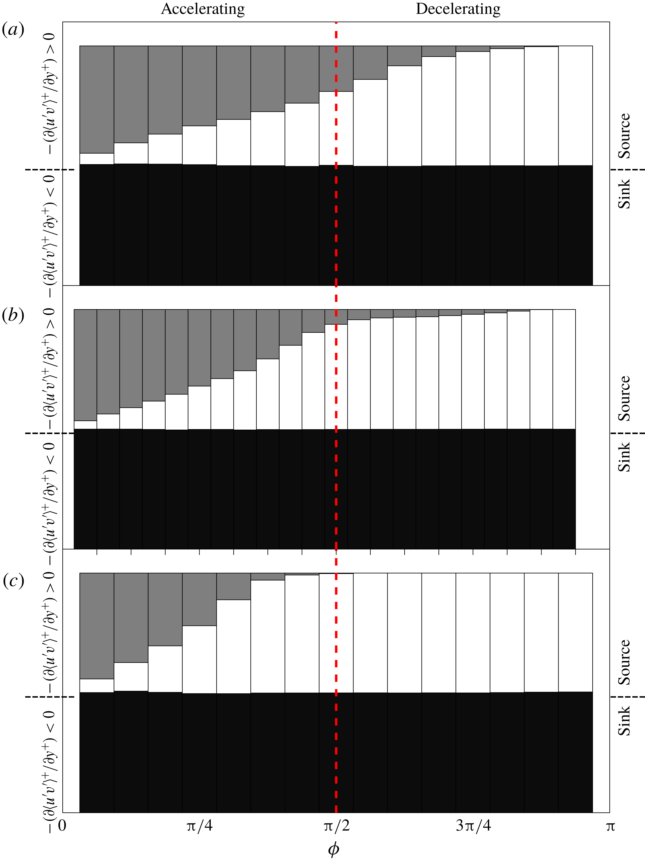
(c). Black is the contribution of the momentum sink, white is the contribution of the ‘wall momentum source’ and grey is the contribution of the ‘centreline momentum source’. The vertical red dashed line separates the accelerating and decelerating phases of the half-period.

A striking feature in OCF is a second momentum source near the channel centreline, most evident during the accelerating portion of the cycle as illustrated in the right panel of figure 7. The existence of this second momentum source is a clear indication that OCF (at least during the portion of the cycle where a second momentum source is observed) is very different compared to its canonical counterpart. Here we term the two source regions in OCF as the ‘wall momentum source’ and ‘centreline momentum source’. Consequently, when the centreline momentum source is of leading-order importance (i.e. non-negligible compared to the wall momentum source), turbulent inertia in OCF redistributes momentum from the interior region of the flow to both the near-wall and centreline regions of the flow. Owing to the evolution of the turbulent inertia in OCF (as given in figure 6), the source- and sink-like regions evolve as function of phase angle and the percentage of momentum transferred to the centreline momentum source compared to the wall momentum source varies throughout the cycle as shown in figure 8.
For
 $Re_{s}=648$
, the centreline momentum source is dominant in the early phases of the accelerating portion of the cycle, it then decreases monotonically with increasing phase angle but remains finite throughout the accelerating portion of the cycle and into the early part of the decelerating portion of the cycle until it becomes negligible (less than 10 % of the wall momentum source) at
 $\unicode[STIX]{x1D719}\approx 11\unicode[STIX]{x03C0}/16$
. The centreline momentum source for
 $Re_{s}=1009$
is also dominant in the early phases of the accelerating portion of the cycle but rapidly decreases with increasing phase angle until it becomes negligible (less than 10 % of the wall momentum source) at
 $\unicode[STIX]{x1D719}\approx 6\unicode[STIX]{x03C0}/16$
. The centreline momentum source for
 $Re_{s}=801$
becomes negligible at
 $\unicode[STIX]{x1D719}\approx 13\unicode[STIX]{x03C0}/24$
. Note that for both the higher
 $Re_{s}$
, the phase angle at which the centreline momentum source loses leading-order importance is nearly identical to the phase angle where a logarithmic mean velocity distribution emerges.
The wall-normal peak location of the Reynolds stress plotted as a function of
 $\unicode[STIX]{x1D719}$
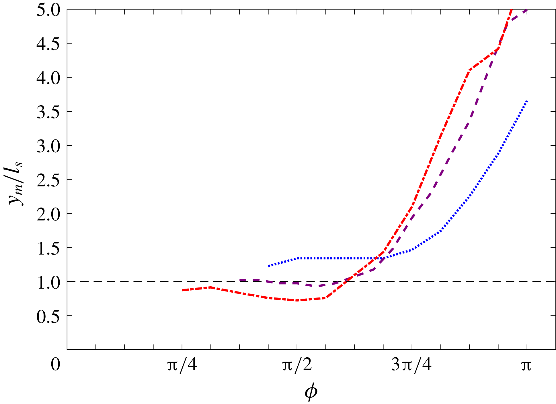
for the phase angles when the integrated contribution from the wall momentum source becomes greater than that of the centreline momentum source. The line styles are the same as in figure 2.

It is reasonable to assume that once the integrated contribution from the wall momentum source becomes greater than that of the centreline momentum source, the flow structure of OCF approaches a flow structure closer resembling that of a steady turbulent channel flow. For these conditions, the wall-normal peak location of the Reynolds stress evaluated as a function of
 $\unicode[STIX]{x1D719}$
is shown in figure 9 for the three
 $Re_{s}$
. Here it is observed that the peak location of the Reynolds stress during the late accelerating portion of the cycle is within the Stokes layer for
 $Re_{s}=1009$
, at the edge of the Stokes layer for
 $Re_{s}=801$
and outside the Stokes layer for
 $Re_{s}=684$
.
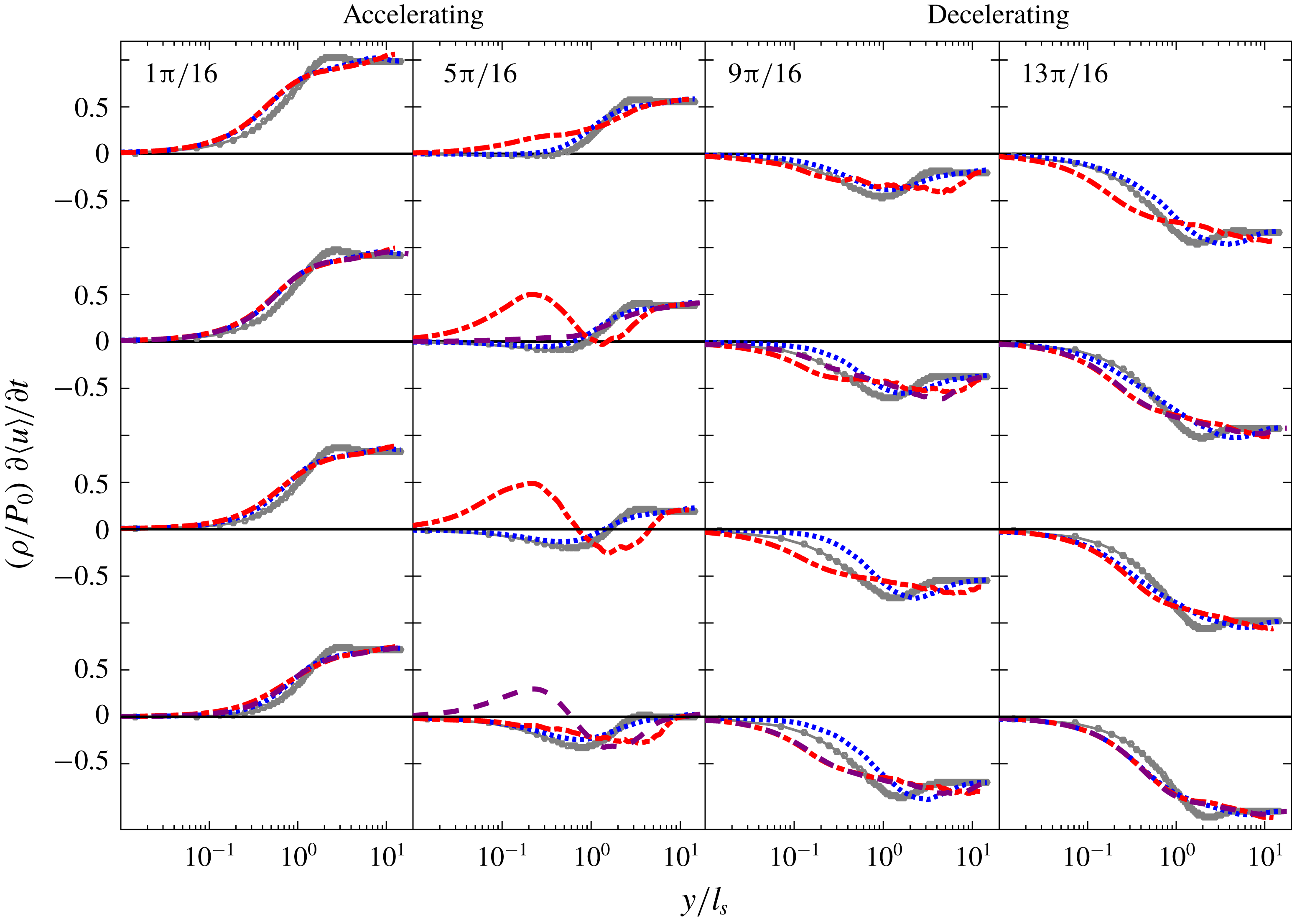
Phase-averaged profiles of the local acceleration plotted as a function of
 $\unicode[STIX]{x1D719}$
. The line styles are the same as in figure 1.

3.4 Evolution of the local acceleration
$(\unicode[STIX]{x2202}\langle u\rangle ^{+}/\unicode[STIX]{x2202}t^{+})$

The evolution of the wall-normal profiles of local acceleration as a function of phase angle is shown in figure 10. The profile of local acceleration analytically computed for laminar OCF is included for baseline comparison. Similar to the profiles of other mean flow quantities presented above, the profiles for the three
 $Re_{s}$
nearly collapse on each other during the early accelerating phase angles (
 $1\unicode[STIX]{x03C0}/16\lesssim \unicode[STIX]{x1D719}\lesssim \unicode[STIX]{x03C0}/4$
) and the late decelerating phase angles (
 $15\unicode[STIX]{x03C0}/16\lesssim \unicode[STIX]{x1D719}\lesssim \unicode[STIX]{x03C0}$
) of the first half-period. The profiles of local acceleration at
 $Re_{s}=648$
closely trend with the laminar profiles across the entire cycle, whereas the profiles of local acceleration at
 $Re_{s}=1009$
begin to trend differently from the laminar profile at
 $\unicode[STIX]{x1D719}\approx 5\unicode[STIX]{x03C0}/16$
. A particularly interesting feature of the
 $Re_{s}=1009$
profile at this phase angle is an apparent kink in the profile at
 $y/l_{s}\approx 1$
. With increasing
 $\unicode[STIX]{x1D719}$
, the kink remains at a fixed wall-normal position but the magnitude on the wallward side of the kink increases while it decreases on its opposite side, producing a profile with a distinct local minimum and maximum that both increase with
 $\unicode[STIX]{x1D719}$
until disappearing at
 $\unicode[STIX]{x1D719}\approx 7\unicode[STIX]{x03C0}/16$
. A similar kinked profile centred at
 $y/l_{s}\approx 1$
is observed for
 $Re_{s}=801$
from
 $6\unicode[STIX]{x03C0}/16\lesssim \unicode[STIX]{x1D719}\lesssim \unicode[STIX]{x03C0}/2$
. Note that the
 $Re_{s}=648$
profile does not show a kinked profile at any point in the cycle. Effectively, the
 $\unicode[STIX]{x2202}\langle u\rangle /\unicode[STIX]{x2202}t$
profiles indicate that during the late phase angles of the acceleration portion of the cycle for both the higher
 $Re_{s}$
there is an internal layer that on the wallward side is locally accelerating and on the opposite side is locally decelerating at a rate that increases with
 $\unicode[STIX]{x1D719}$
. Close inspection of the mean velocity profiles in figure 2 supports these behaviours.
The emergence and development of an internal layer centred at
 $y/l_{s}\approx 1$
during the late phase angles of the accelerating portion of the cycle (just prior to when fully turbulent characteristics are observed) may be implicitly inferred from previous findings in the literature. Specifically, since the viscous term outside the Stokes layer is small (scaling like
 $Re_{s}^{-1}$
), the unsteady term is the only term that can respond to the explosive growth of turbulent inertia. Furthermore, the emergence of the internal layer may be related to the emergence and phase evolution of local extrema (and corresponding adjacent inflection points) in the phased-averaged mean velocity profile, as detailed by Spalart & Baldwin (Reference Spalart and Baldwin1989).
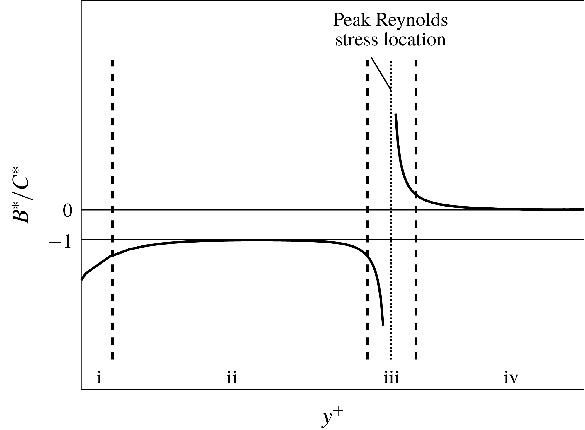
Sketch of the four layer structure of steady turbulent channel flow at a representative, large Reynolds number: region i
 $|A^{\ast }|\simeq |B^{\ast }|\gg |C^{\ast }|$
; region ii
 $|B^{\ast }|\simeq |C^{\ast }|\gg |A^{\ast }|$
; region iii
 $|A^{\ast }|\simeq |B^{\ast }|\simeq |C^{\ast }|$
; region iv
 $|A^{\ast }|\simeq |C^{\ast }|\gg |B^{\ast }|$
(Wei et al.
Reference Wei, Fife, Klewicki and Mcmurtry2005).

3.5 Four layer structure in the mean momentum balance
Equation (3.2) is effectively the time-averaged statement of Newton’s second law for a differential fluid element, and as such must be locally satisfied over
 $0\leqslant y\leqslant h$
. For steady turbulent channel flow, term
 $D^{\ast }$
is zero and the ratio
 $B^{\ast }/C^{\ast }$
best exposes how the balance is realized, as shown in figure 11, which depicts the four layer structure of wall-bounded turbulent flow (Wei et al.
Reference Wei, Fife, Klewicki and Mcmurtry2005; Klewicki, Fife & Wei Reference Klewicki, Fife and Wei2009). Within three of these regions, the mean momentum equation is brought into balance with two large terms dominating one small term (regions
 $\text{i}$
,
 $\text{ii}$
and
 $\text{iv}$
), while in another region (region
 $\text{iii}$
), all three terms contribute significantly to the balance. Thus, while all of the three terms are of leading-order importance over some portion of the wall-normal domain, in three of the four regions there emerges only two dominant terms.
The ratio of the gradient of the viscous stress (
 $B^{\ast }$
) to the Reynolds stress gradient (
 $C^{\ast }$
) as a function of
 $\unicode[STIX]{x1D719}$
in OCF for the three
 $Re_{s}$
. A four layer structure is observed from
 $6\unicode[STIX]{x03C0}/16\lesssim \unicode[STIX]{x1D719}\lesssim 11\unicode[STIX]{x03C0}/16$
and
 $8\unicode[STIX]{x03C0}/16\lesssim \unicode[STIX]{x1D719}\lesssim 10\unicode[STIX]{x03C0}/16$
for
 $Re_{s}=1009$
and
 $Re_{s}=801$
, respectively.

For OCF, a single ratio to expose the balance is insufficient owing to the four non-zero terms in (3.2). Moreover, these terms will vary with
 $\unicode[STIX]{x1D719}$
over an oscillation period. Nevertheless, it is worthwhile to evaluate if a four layer structure emerges for the two higher
 $Re_{s}$
since empirical and theoretical evidence suggests that the formation of a four layer structure is an important characteristic of a self-similar hierarchal structure that underlies logarithmic dependence of the mean velocity profile in steady turbulent wall-bounded flows (Wei et al.
Reference Wei, Fife, Klewicki and Mcmurtry2005; Klewicki et al.
Reference Klewicki, Fife and Wei2009; Klewicki & Oberlack Reference Klewicki and Oberlack2015). Figure 12 shows the ratio
 $B^{\ast }/C^{\ast }$
in OCF as a function of
 $\unicode[STIX]{x1D719}$
for the three
 $Re_{s}$
. It is both informative and theoretically interesting that a four layer structure emerges for
 $Re_{s}=801$
and 1009 at the precise phase angles where the turbulent characteristics in OCF are similar to that of steady wall-bounded turbulent flows. Note that a four layer structure is not observed for
 $Re_{s}=648$
during any part of the cycle. The theoretical implications of these findings are not be pursued in the present study.
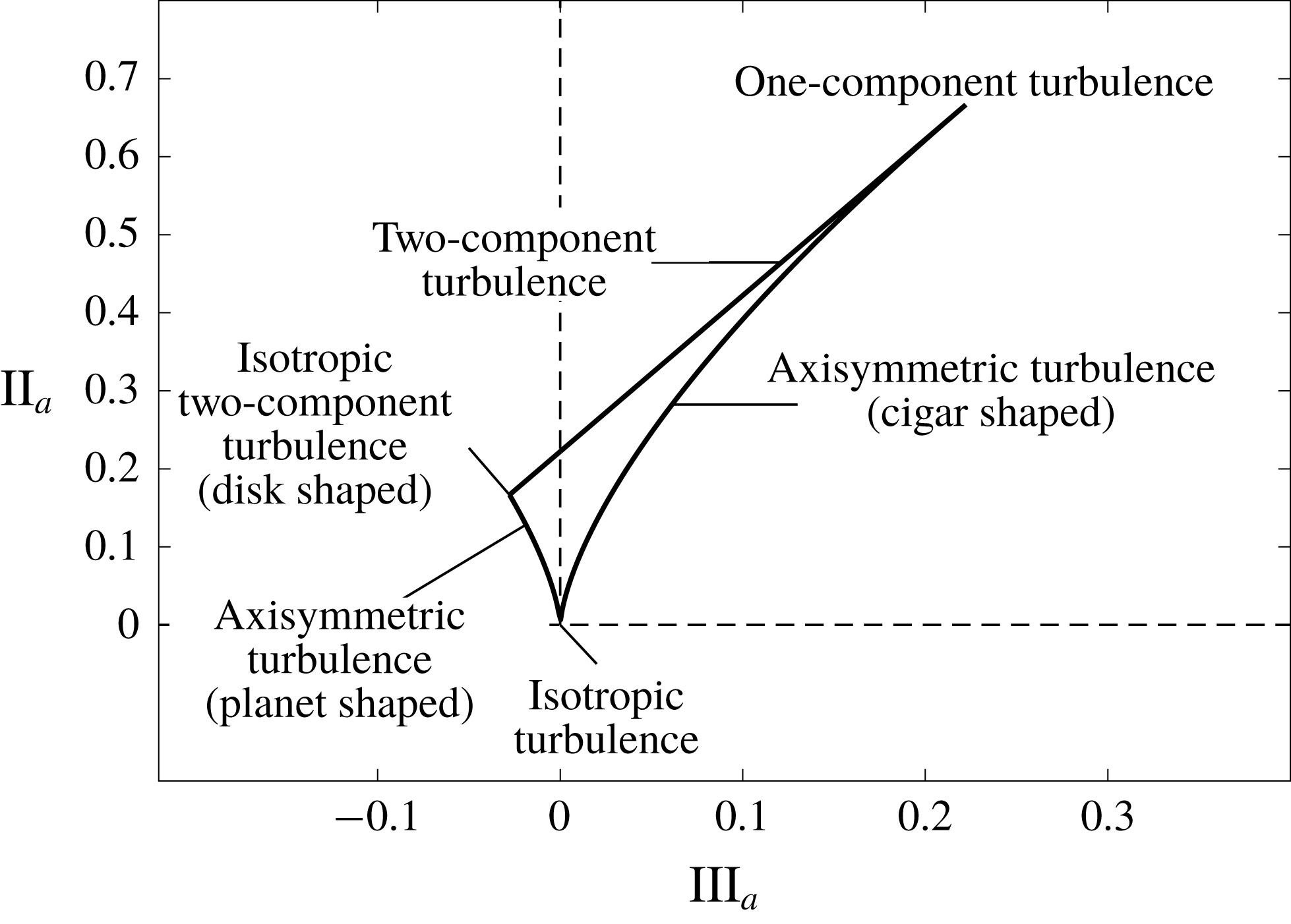
Anisotropy invariant map showing the limiting state of turbulence.

3.6 Turbulent structure in OCF
The wall-normal turbulent structure in OCF as a function of
 $\unicode[STIX]{x1D719}$
and
 $Re_{s}$
is evaluated from the anisotropy invariant map introduced by Lumley & Newman (Reference Lumley and Newman1977), which employs the anisotropy tensor given by
 $$\begin{eqnarray}\unicode[STIX]{x1D623}_{ij}=\frac{\langle u_{i}^{\prime }u_{j}^{\prime }\rangle }{q^{2}}-\frac{1}{3}\unicode[STIX]{x1D6FF}_{ij},\end{eqnarray}$$
where
 $q^{2}=\langle u_{i}^{\prime }u_{i}^{\prime }\rangle$
. The three scalar scalar invariants of the tensor are
 $$\begin{eqnarray}\displaystyle & \displaystyle \text{I}_{a}=0, & \displaystyle\end{eqnarray}$$
 $$\begin{eqnarray}\displaystyle & \displaystyle \text{II}_{a}=\unicode[STIX]{x1D623}_{ij}\unicode[STIX]{x1D623}_{ji}, & \displaystyle\end{eqnarray}$$
and
 $$\begin{eqnarray}\text{III}_{a}=\unicode[STIX]{x1D623}_{ij}\unicode[STIX]{x1D623}_{jk}\unicode[STIX]{x1D623}_{ki}.\end{eqnarray}$$
The anisotropy invariant map is produced by plotting
 $\text{II}_{a}$
versus
 $\text{III}_{a}$
(Lumley & Newman Reference Lumley and Newman1977; Jovanović & Hillerbrand Reference Jovanović and Hillerbrand2005; Simonsen & Krogstad Reference Simonsen and Krogstad2005; Frohnapfel et al.
Reference Frohnapfel, Lammers, Jovanović and Durst2007). Figure 13 shows the bounding limits of the anisotropy invariant map for all physically realizable turbulence. The turbulent structure is quantified by the shape of the stress tensor at a given state on the anisotropy invariant map (Simonsen & Krogstad Reference Simonsen and Krogstad2005). The origin
 $(0,0)$
represents three-component isotropic turbulence with a spherical stress tensor. The left and right limiting curves originating at the origin are given by
 $$\begin{eqnarray}\text{II}_{a}={\textstyle \frac{3}{2}}\left({\textstyle \frac{4}{3}}|\text{III}_{a}|\right)^{2/3}.\end{eqnarray}$$
The left-hand curve represents axisymmetric two-component turbulence where one component has a smaller magnitude than the other two, and the stress tensor shape is described as an oblate spheroid (planet like). The limiting value of the left-hand curve is two-component axisymmetric turbulence (disc-shaped stress tensor). The right-hand curve represents the other kind of axisymmetric turbulence where one component is larger than the other two, and the stress tensor shape is described as prolate spheroid (cigar like). The limiting value of the right-hand curve is one-component turbulence. The straight line connecting the two limiting values of the axisymmetric turbulence curves given by
 $$\begin{eqnarray}\text{II}_{a}={\textstyle \frac{2}{9}}+2\text{III}_{a},\end{eqnarray}$$
represents two-component turbulence (ellipse-shaped stress tensor), where one term is zero and one term increases in magnitude as the one-component turbulence limit is approached (Lumley & Newman Reference Lumley and Newman1977; Simonsen & Krogstad Reference Simonsen and Krogstad2005). This type of two-component turbulence exists within the viscous sublayer in wall-bounded turbulent flow.
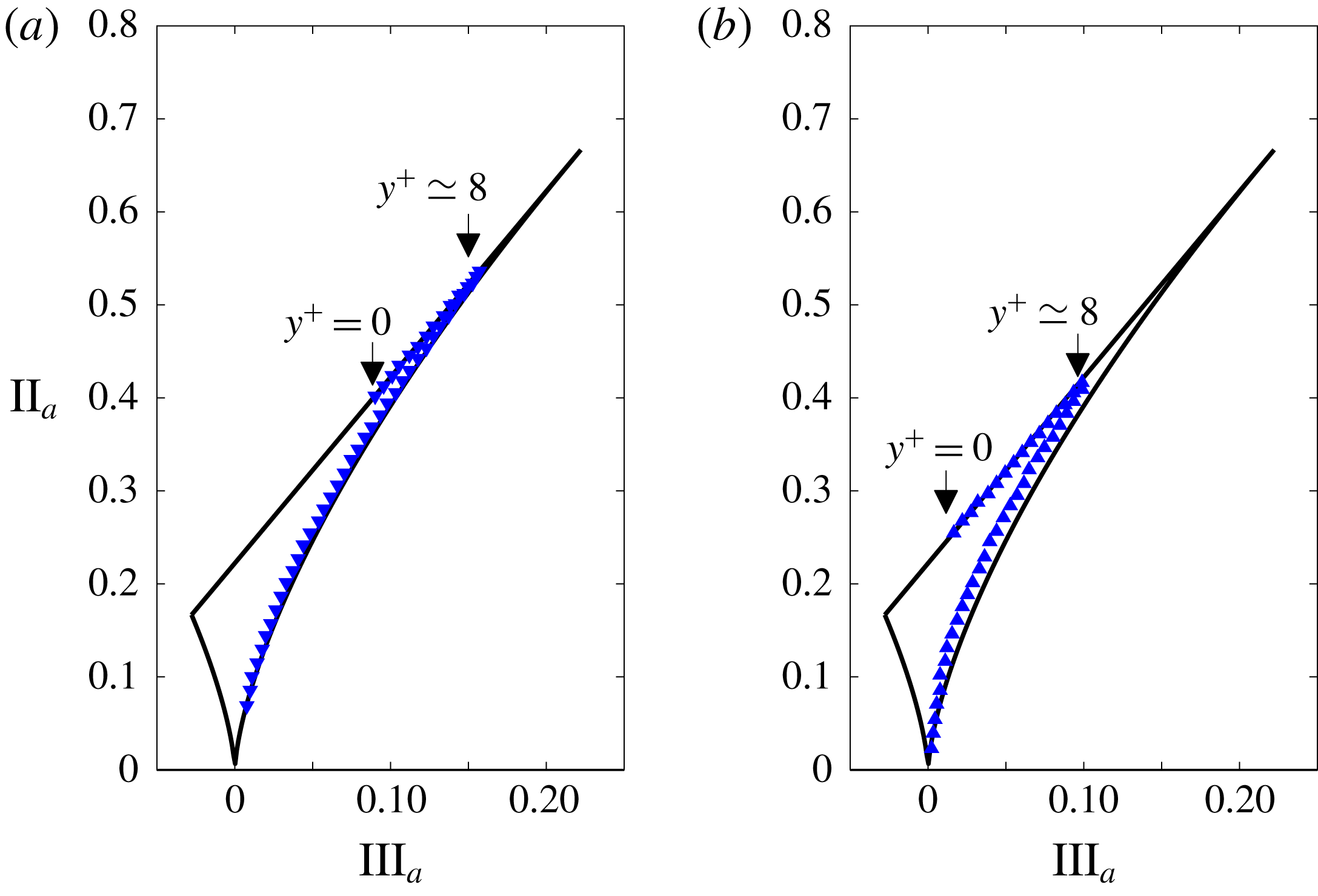
Anisotropy invariant map in steady turbulent channel flow at (a)
 $Re_{\unicode[STIX]{x1D70F}}=100$
(Kuroda Reference Kuroda1990) and (b)
 $Re_{\unicode[STIX]{x1D70F}}=590$
(Moser, Kim & Mansour Reference Moser, Kim and Mansour1999). The data are extracted from Frohnapfel et al. (Reference Frohnapfel, Lammers, Jovanović and Durst2007).

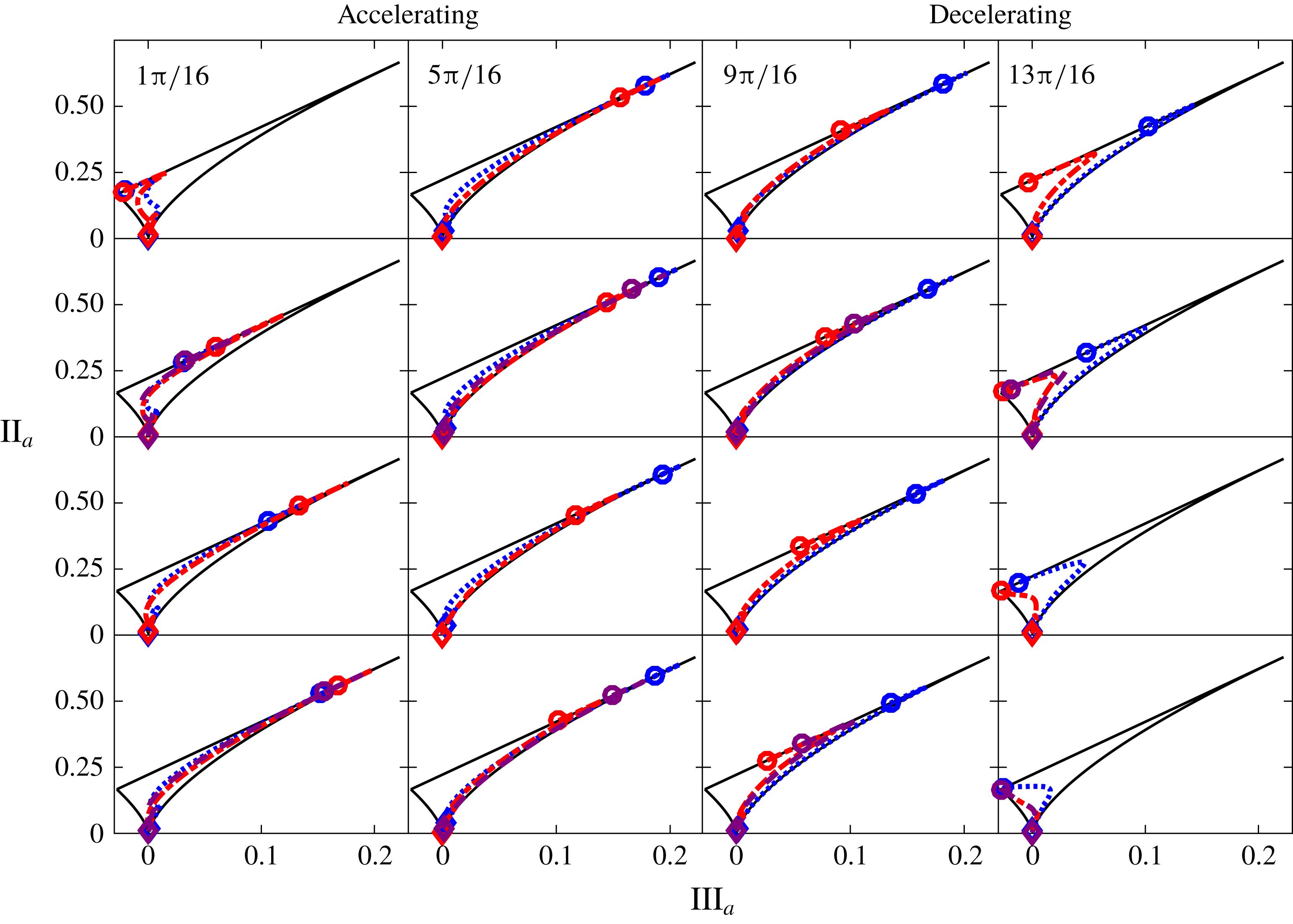
Anisotropy invariant map in OCF. The line styles are the same as in figure 2. The open circles denote
 $y=0$
and the open diamonds denote
 $y=h$
. The wall-normal location increases moving from the open circles to the open diamonds.

Anisotropy invariant maps computed from steady turbulent channel flow at
 $Re_{\unicode[STIX]{x1D70F}}=100$
and
 $Re_{\unicode[STIX]{x1D70F}}=590$
are shown in figure 14. The flow in the near-wall region (
 $y^{+}\lesssim 8$
) lies on or close to the straight line corresponding to two-component turbulence. The effect of increasing
 $Re_{\unicode[STIX]{x1D70F}}$
is to decrease the anisotropy in the near-wall region such as to move the flow farther from one-component turbulence. For
 $y^{+}\gtrsim 8$
, the streamwise fluctuations are large compared to the non-negligible transverse components and the axisymmetric turbulence stress tensor is cigar shaped. The effect of increasing
 $Re_{\unicode[STIX]{x1D70F}}$
is to decrease the anisotropy such that the data shift to the left of the right-hand limiting curve. As a consequence of decreasing anisotropy in the interior of the flow, the turbulence near the centreline at the higher
 $Re_{\unicode[STIX]{x1D70F}}$
is more isotropic than that at the lower
 $Re_{\unicode[STIX]{x1D70F}}$
.
The anisotropy maps in OCF computed at each
 $\unicode[STIX]{x1D719}$
for the three
 $Re_{s}$
are shown in figure 15. In these plots, the open circles denote
 $y=0$
and the open diamonds denote
 $y=h$
such that the wall-normal location on the anisotropy invariant map increases, moving from the open circle to the open diamond. At the start of the accelerating portion (
 $\unicode[STIX]{x1D719}=(\unicode[STIX]{x03C0}/16)$
) of the cycle, the turbulence is two-component axisymmetric disk shaped near the wall and approaches three-component isotropic turbulence near the centreline. As the flow accelerates, the anisotropy near the wall increases, and the near-wall turbulence moves toward one-component turbulence consistent with the emergence and the strengthening of streamwise velocity streaks. With increasing
 $\unicode[STIX]{x1D719}$
, the shift of the near-wall turbulence away from one-component turbulence (towards the axisymmetric two-component turbulence limiting point) is indicative of streak breakdown and the onset of the nonlinear development stage. This downward shift is observed to occur at
 $\unicode[STIX]{x1D719}\approx 6\unicode[STIX]{x03C0}/16,8\unicode[STIX]{x03C0}/16,10\unicode[STIX]{x03C0}/16$
for
 $Re_{s}=1009,801,648$
, respectively. This is consistent with the phase angle corresponding to the rapid growth of the Reynolds stress and its wall-normal gradient, and, for the two higher
 $Re_{s}$
, the emergence of a locally accelerating/decelerating internal layer and the rapid rise in
 $C_{f}$
as observed in the data presented above. During the decelerating portion of the cycle, the anisotropy invariant maps show that the near-wall anisotropy decreases and the near-wall turbulence moves toward the axisymmetric two-component turbulence limiting point. The convergence to the two-component turbulence limiting point occurs at an earlier phase angle for increasing
 $Re_{s}$
.
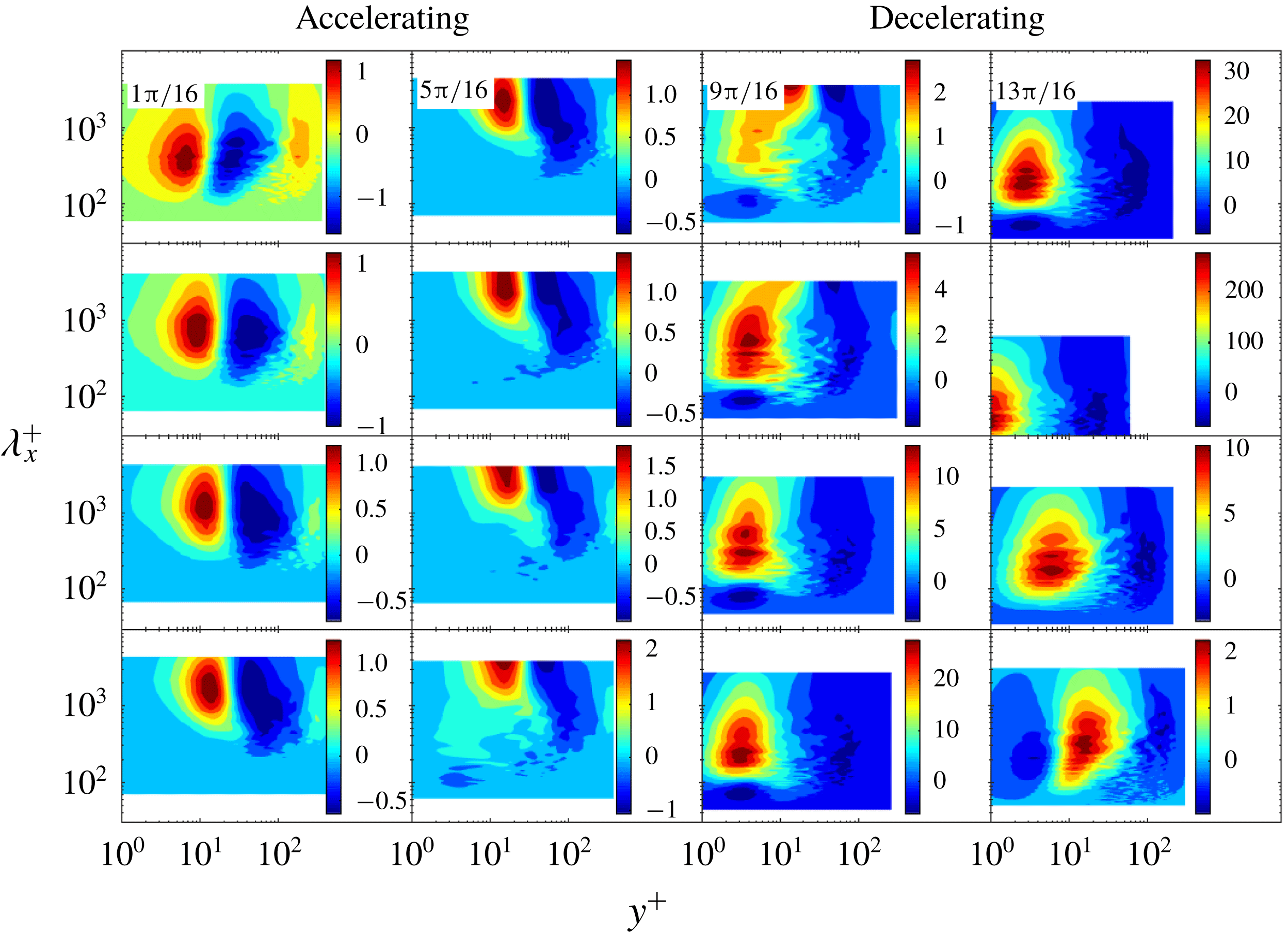
3.7 Co-spectra
Phase evolution of the spectrograms of the premultiplied co-spectra of the Reynolds stress gradient
 $k_{x}^{+}\unicode[STIX]{x2202}\unicode[STIX]{x1D6F7}_{-u^{\prime }v^{\prime }}^{+}/\unicode[STIX]{x2202}y^{+}$
at
 $Re_{s}=648$
as a function of streamwise wavelength
 $\unicode[STIX]{x1D706}^{+}$
and wall distance
 $y^{+}$
, where
 $k_{x}$
is the streamwise wavenumber.

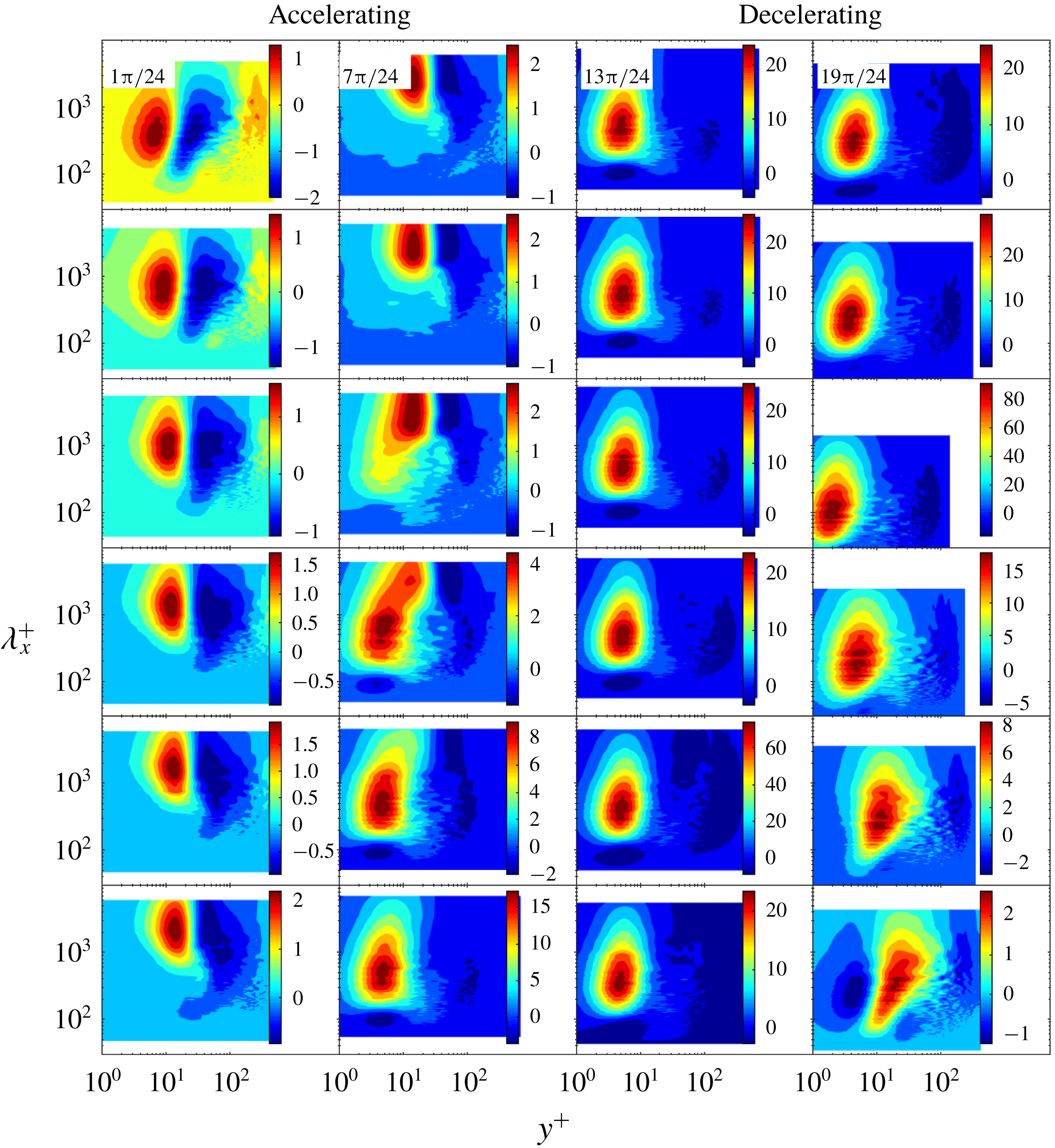
Phase evolution of the spectrograms of the premultiplied co-spectra of the Reynolds stress gradient
 $k_{x}^{+}\unicode[STIX]{x2202}\unicode[STIX]{x1D6F7}_{-u^{\prime }v^{\prime }}^{+}/\unicode[STIX]{x2202}y^{+}$
at
 $Re_{s}=801$
as a function of streamwise wavelength
 $\unicode[STIX]{x1D706}^{+}$
and wall distance
 $y^{+}$
, where
 $k_{x}$
is the streamwise wavenumber.

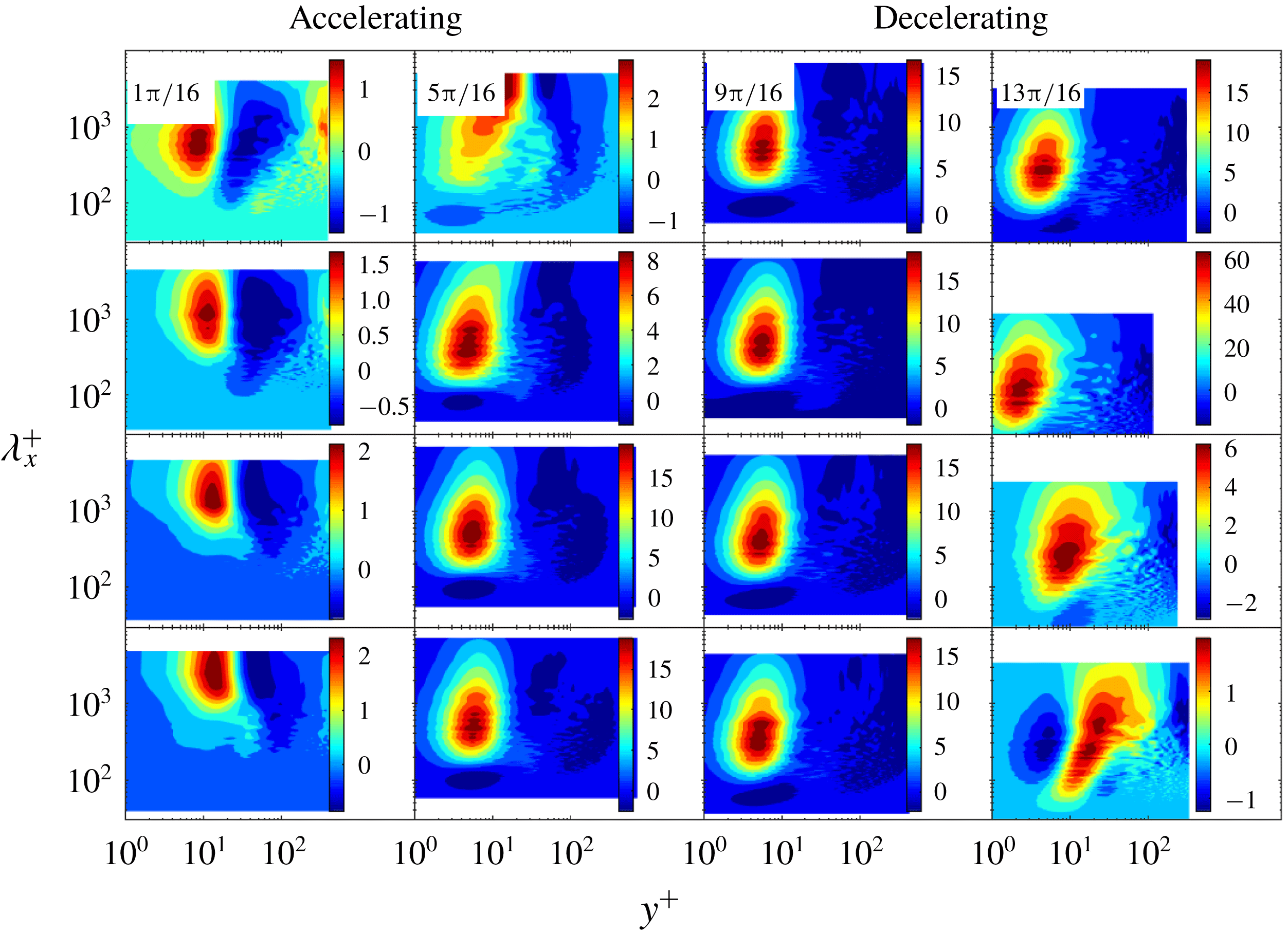
Phase evolution of the spectrograms of the premultiplied co-spectra of the Reynolds stress gradient
 $k_{x}^{+}\unicode[STIX]{x2202}\unicode[STIX]{x1D6F7}_{-u^{\prime }v^{\prime }}^{+}/\unicode[STIX]{x2202}y^{+}$
at
 $Re_{s}=1009$
as a function of streamwise wavelength
 $\unicode[STIX]{x1D706}^{+}$
and wall distance
 $y^{+}$
, where
 $k_{x}$
is the streamwise wavenumber.

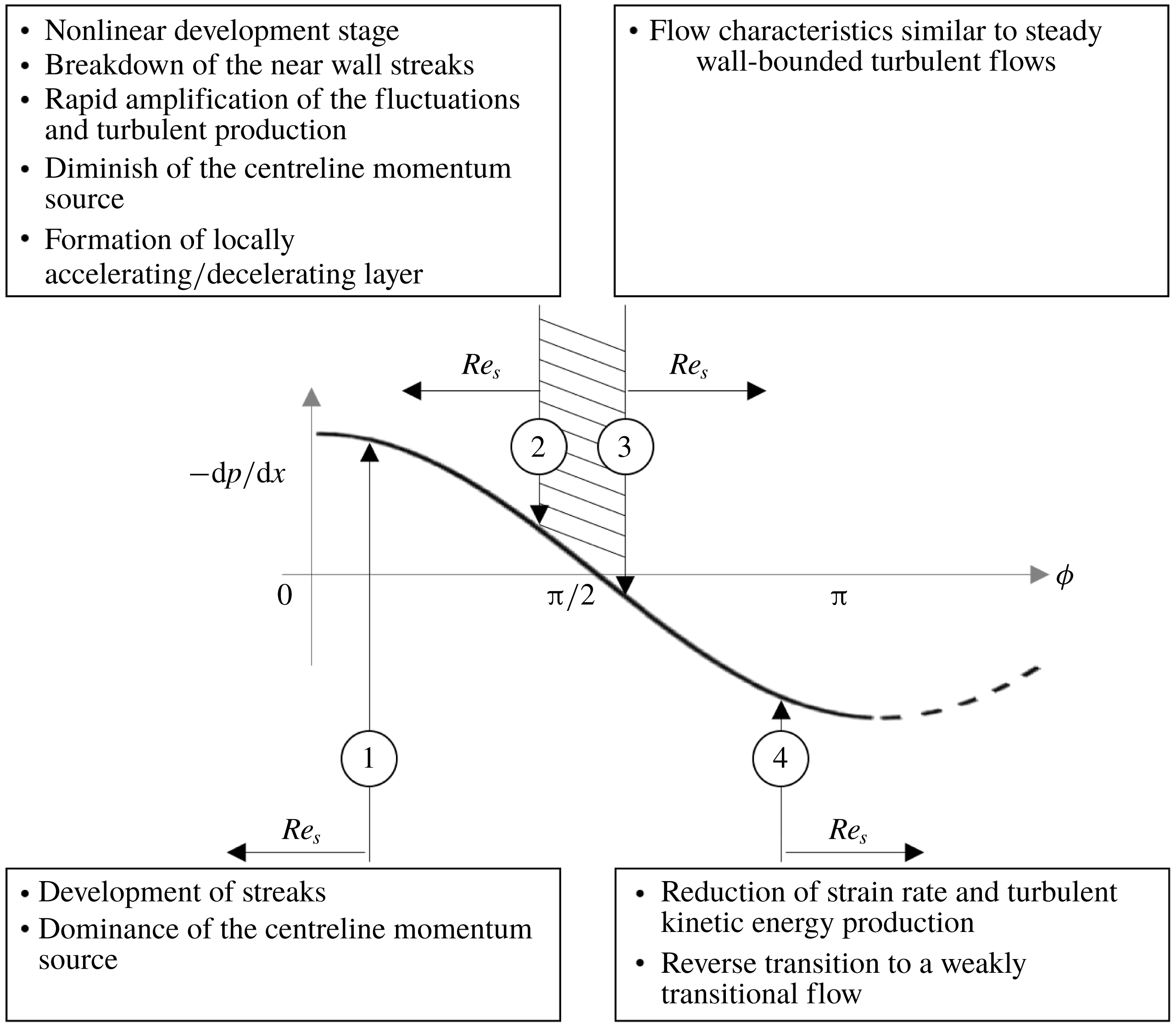
Schematic of the stages of transition to turbulence in OCF over a half-period of oscillation. Critical to transition to turbulence is that the nonlinear development stage begins during the acceleration portion of the cycle.

Further insights regarding the mean flow dynamics in OCF are gained by examining spectral characteristics associated with the turbulent inertia. Figures 16–18 show the phase angle evolution of the spectrograms of the premultiplied co-spectra of the Reynolds stress gradient
 $k_{x}^{+}\unicode[STIX]{x2202}\unicode[STIX]{x1D6F7}_{-u^{\prime }v^{\prime }}^{+}/\unicode[STIX]{x2202}y^{+}$
for
 $Re_{s}=648$
,
 $Re_{s}=801$
and
 $Re_{s}=1009$
, respectively, as a function of streamwise wavelength
 $\unicode[STIX]{x1D706}^{+}$
and wall-normal distance
 $y^{+}$
, where
 $k_{x}$
is the streamwise wavenumber. Blue regions in the spectrograms represent strong momentum sink-like regions, red regions represent strong momentum source-like regions (Chin et al.
Reference Chin, Philip, Klewicki, Ooi and Marusic2014) and the positive and the negative areas of the spectrograms sum to zero. Effectively, momentum is transported from red regions to blue regions by turbulent inertia, with contributions from different
 $\unicode[STIX]{x1D706}^{+}$
as described by the spectrogram. Interpreted as a force term in the momentum equation, source-like regions will accelerate the flow and sink-like regions will decelerate the flow (Wu, Baltzer & Adrian Reference Wu, Baltzer and Adrian2012).
The spectrograms show that in the first half of the accelerating phases of the cycle (
 $1\unicode[STIX]{x03C0}/16\lesssim \unicode[STIX]{x1D719}\lesssim \unicode[STIX]{x03C0}/4$
) the co-spectra are nearly identical for the three
 $Re_{s}$
. While in the second half of the accelerating phases of the cycle, the co-spectra differ significantly between the lower
 $Re_{s}$
and the two higher
 $Re_{s}$
. In particular, for
 $Re_{s}=648$
the wall momentum source moves upward with increasing phase during the accelerating portion of the cycle, indicating an increase in the characteristic turbulent length scales associated with the transport of momentum with increasing phase. In the decelerating portion of the cycle, the wall momentum source moves down and to the left from
 $\unicode[STIX]{x1D719}=9\unicode[STIX]{x03C0}/16$
to
 $\unicode[STIX]{x1D719}=10\unicode[STIX]{x03C0}/16$
indicating that the peak in the Reynolds stress moves closer to the wall and that the characteristic turbulent length scales associated with the transport of momentum have decreased. Interestingly, the phase angle where the peak in the Reynolds stress moves closer to the wall is approximately at the same phase angle where the centreline momentum source loses leading-order importance. For
 $Re_{s}=1009$
, the wall momentum source moves down and to the left from
 $\unicode[STIX]{x1D719}=5\unicode[STIX]{x03C0}/16$
to
 $\unicode[STIX]{x1D719}=6\unicode[STIX]{x03C0}/16$
indicating that the peak in the Reynolds stress moves closer to the wall during the accelerating portion of the cycle. This is consistent with phase angle corresponding to a rapid rise in
 $C_{f}$
(see figure 1) and indicative of the onset of the nonlinear development stage. Again, the phase angle at which this occurs is approximately at the same phase angle where the centreline momentum source losses leading-order importance. Then, during the late accelerating phases and early decelerating phases of the cycle (
 $7\unicode[STIX]{x03C0}/16\lesssim \unicode[STIX]{x1D719}\lesssim 14\unicode[STIX]{x03C0}/16$
), the co-spectra are qualitatively similar from phase to phase. Note that these co-spectra are also qualitatively similar to the co-spectra of the Reynolds stress gradient in steady turbulent pipe flow (Wu et al.
Reference Wu, Baltzer and Adrian2012; Chin et al.
Reference Chin, Philip, Klewicki, Ooi and Marusic2014). Not surprising, these phases coincide with the phases where a logarithmic region in the mean velocity profile is observed. Importantly, the wallward movement of the wall momentum source from
 $\unicode[STIX]{x1D719}=5\unicode[STIX]{x03C0}/16$
to
 $\unicode[STIX]{x1D719}=6\unicode[STIX]{x03C0}/16$
coincides with the emergence of the internal layer as described in the evolution of the local acceleration. Also observed in figure 18 is a small island of momentum sink from
 $y^{+}\approx 2{-}8$
and
 $\unicode[STIX]{x1D706}^{+}<100$
that first emerges at
 $\unicode[STIX]{x1D719}=5\unicode[STIX]{x03C0}/16$
. Similar observations to the
 $Re_{s}=1009$
spectrograms can be made from the
 $Re_{s}=801$
spectrograms.
4 Discussion and conclusions
A description of the mean dynamics in OCF and the evolution of this dynamics through transition were provided in the data presentation. In this section, we describe the implications related to the dynamical mechanisms of transition to turbulence in OCF and a brief summary of key findings.
4.1 Dynamical mechanism of transition to turbulence
Figure 19 is a schematic of the stages of transition to turbulence in OCF over a half-period of oscillation based on the authors’ interpretation of the present results and results from previous studies in the literature (Akhavan et al. Reference Akhavan, Kamm and Shapiro1991b ; Elsnab et al. Reference Elsnab, Klewicki, Maynes and Ameel2011; Klewicki, Ebner & Wu Reference Klewicki, Ebner and Wu2011; Ozdemir et al. Reference Ozdemir, Hsu and Balachandar2014). While the mechanisms described below are physically consistent with the data, since they are based only on limited observations of the mean dynamics; further studies are required to fully understand the transition mechanism in oscillatory flow. The present description therefore should be viewed only as a framework to better understand transition to turbulence in OCF.
During the initial accelerating phases of the cycle
 $\unicode[STIX]{x2460}$
, near-wall velocity streaks form and the near-wall turbulence approaches a one-component dominant state as evidenced by the phase evolution of the r.m.s. fluctuating velocity profiles (figure 4) and the anisotropy invariant map (figure 15). At
 $Re_{s}\geqslant 750$
, the nonlinear development stage (i.e. streak breakdown) begins during the accelerating portion of the cycle and its growth rate is fast enough such that Reynolds stress and its divergence explosively increase prior to the start of the decelerating portion of the cycle, as observed in figures 5 and 6 for the two higher
 $Re_{s}~\unicode[STIX]{x2461}$
. The evidence of the nonlinear development stage is observed by the rapid growth of
 $v^{\prime }$
and
 $w^{\prime }$
in the near-wall region, the shift away from one-component turbulence in the anisotropy invariant map and the shift of the wall momentum source down (to smaller wavelength) and to the left (towards the wall) in the co-spectra (figure 18) of the Reynolds stress gradient, among other measures provided in the data presentation. The explosive growth of the near-wall Reynolds stress gradient leads to its increasing importance in the mean momentum balance and the decreasing importance of the centreline momentum source. This explosive growth is accompanied by the wall-normal rearrangement of the local mean acceleration and the mean viscous force. Specifically, on the wallward side of the peak in the Reynolds stress (i.e. at the zero crossing of the Reynolds stress gradient) the flow locally accelerates and decelerates on its opposite side and the viscous force increases near the wall. This rearrangement of forces culminates in the emergence of a four layer structure in the mean balance of forces, as shown in figure 12, typical of fully developed turbulent wall-bounded flows. A similar conclusion that during transition to turbulence there is a wall-normal rearrangement of the mean momentum balance culminating in the four layer structure was reported by Elsnab et al. (Reference Elsnab, Klewicki, Maynes and Ameel2011) for transition in channel flow and Klewicki et al. (Reference Klewicki, Ebner and Wu2011) for transition in ZPG boundary layer flow.
The turbulence, with characteristics similar to steady wall-bounded turbulent flows, is self-sustaining over a duration of the cycle, where this duration increases with increasing
 $Re_{s}~\unicode[STIX]{x2462}$
. Then, during the later decelerating portion of the cycle
 $\unicode[STIX]{x2463}$
, the strain rate is reduced, the production of turbulent kinetic energy is diminished and the self-sustaining process is terminated. The flow then proceeds through a reverse transition and returns to a weakly transitional state at the end of the decelerating portion of the cycle. This process is repeated indefinitely. The fundamental implications of transition in OCF, as described here, is that since the process is repeatable (at least in the mean sense) and has many elements similar to transition in channel flow and ZPG boundary layer flow, it is therefore more amenable than its canonical counterparts to physical observations aimed at understanding transition to turbulence in wall-bounded flows.
4.2 Summary
Data from direct numerical simulation studies of oscillatory channel flow were used to examine the phase evolution of the mean dynamics for a self-sustaining transitional flow (
 $Re_{s}=648$
) and two intermittently turbulent flows (
 $Re_{s}=801$
and 1009). One primary finding of the data analysis is that transition to turbulence results when the nonlinear development stage begins during the accelerating portion of the cycle. This is in agreement with Akhavan et al. (Reference Akhavan, Kamm and Shapiro1991b
) and Ozdemir et al. (Reference Ozdemir, Hsu and Balachandar2014) who both report the ‘explosive growth of turbulence activity’ towards the end of the accelerating portion of the cycle due to the nonlinear breakdown of flow instabilities. When the nonlinear development stage begins during the decelerating portion of the cycle (i.e. at
 $Re_{s}=648$
), the flow remains weakly transitional over the entire cycle. The absence of transition despite streak breakdown is simply because the nonlinear development stage commences too late in the cycle when the flow is decelerating and the strain rate is diminishing.
The distinguishing contribution of the present study is that the ‘explosive growth of turbulence activity’ has been directly connected to the mean dynamics. Specifically, similar to transition in steady channel flow (Elsnab et al. Reference Elsnab, Klewicki, Maynes and Ameel2011) and ZPG boundary layer flow (Klewicki et al. Reference Klewicki, Ebner and Wu2011), the present results show that the rearrangement of the mean forces during the nonlinear breakdown stage coincides with the explosive growth of the near-wall Reynolds stress and its gradient and the diminishing importance of the centreline momentum source. This is accompanied by the emergence of a locally accelerating/decelerating internal layer near the wall that is observable in the phase-averaged mean. Both the centreline momentum source and the accelerating/decelerating internal layer, to the authors’ knowledge, are unique to OCF. However, similar to transition in steady channel flow and ZPG boundary flow, the wall-normal rearrangement of mean forces culminates in a four layer structure in the mean balance of forces. This is of fundamental importance since the four layer structure is known to be an important characteristic of a similarity hierarchal structure that underlies logarithmic dependence of the mean velocity profile in steady wall-bounded turbulent flows (Wei et al. Reference Wei, Fife, Klewicki and Mcmurtry2005; Klewicki et al. Reference Klewicki, Fife and Wei2009). In this respect, the emergence of a four layer structure appears to be a an excellent metric to evaluate if a wall-bounded flow has transitioned to turbulence.
Acknowledgements
This study was supported by a National Science Foundation/Department of Energy Partnership award nos. 1258702 and 1258697. The authors are thankful to Y. Li et al. (Johns Hopkins Turbulence Database) for providing access to their data.