2.1 Monochromatic regime

To illustrate the origin of the oscillations along the focal line, we consider, for simplicity, a radially symmetric and monochromatic top-hat beam with intensity ${I}_0$ and an angular frequency $\omega$ , incident on an axiparabola mirror. We also allow for the possibility that the mirror includes a central hole of radius ${r}_\mathrm{h}$ , as required in certain applications^[ Reference Durfee and Milchberg ^{3 ,} Reference Oubrerie, Leblanc, Kononenko, Lahaye, Andriyash, Gautier, Goddet, Martelli, Tafzi, Phuoc, Smartsev and Thaury ^{4 ]}. The mirror imprints a radial phase $\phi (r)$ on the beam, thereby focusing rays originating from different radial positions $r$ to distinct axial positions $z(r)$ , where $z=0$ corresponds to the mirror surface. In the Fresnel diffraction regime, the electric field $E$ along the focal line is given by the following:

(1) $$\begin{align}E\left({r}_{\zeta },z\right)=-i\frac{kE_0}{z}{e}^{ik\left(z+\frac{r_{\zeta}^2}{2z}\right)}{\int}_{r_\mathrm{h}}^R{r\mathrm{d}re}^{i\Psi (r)}{J}_0\left(k\frac{r_{\zeta }r}{z}\right),\end{align}$$

where ${r}_{\zeta }$ is the radial position, $k=\omega /c$ , $\Psi (r)={kr}^2/2z-\phi (r)$ and $R$ is the beam radius on the mirror surface^[ Reference Oubrerie, Andriyash, Lahaye, Smartsev, Malka and Thaury ^{14 ]}.

Since ${e}^{i\Psi (r)}$ is a rapidly oscillating function, the integral can be approximated using the stationary-phase method. This method assumes that contributions to the integral cancel out due to destructive interference, except near stationary-phase points, where ${\Psi}^{\prime }(r)=0$ , allowing the integral to be approximated by its local behavior around these points. To this end, we perform a Taylor expansion of the phase around the stationary point ${r}_\mathrm{s}(z)$ , where ${\Psi}^{\prime}\left({r}_\mathrm{s}\right)=0$ . The on-axis field can then be expressed as follows:

(2) $$\begin{align}E\left(0,z\right)=-i\frac{kr_\mathrm{s}}{z}{E}_0{e}^{ikz+i\Psi \left({r}_\mathrm{s}\right)}{\int}_{r_\mathrm{h}}^R{\mathrm{d}re}^{i{\Psi^{\prime}}^{\prime}\left({r}_\mathrm{s}\right){\left(r-{r}_\mathrm{s}\right)}^2/2}.\end{align}$$

Note that, in an optical geometry approach, ${r}_\mathrm{s}(z)$ would represent the radius on the axiparabola mirror of rays that intersect the optical axis at $z$ .

The integration of Equation (2) reduces to evaluating an integral of the form ${\int}_a^b{e}^{i\alpha {r}^2} \mathrm{d}r,$ with $a<0<b$ , which can be approximated as follows:

(3) $$\begin{align}{\int}_a^b{e}^{i\alpha {r}^2} \mathrm{d}r=\sqrt{\frac{\pi }{\alpha }}{e}^{i\pi /4}+i\left(\frac{e^{i\alpha {a}^2}}{2\alpha a}-\frac{e^{i\alpha {b}^2}}{2\alpha b}\right)+\mathcal{O}\left(\frac{1}{\alpha^2}\right).\end{align}$$

In general, in the stationary-phase approach, only the first term is retained, so the on-axis field simplifies to the following:

(4) $$\begin{align}E(z)=-{iE}_0\frac{kr_\mathrm{s}}{z}\sqrt{\frac{2\pi }{{\Psi^{\prime}}^{\prime}\left({r}_\mathrm{s}\right)}}{e}^{i\left( kz+\Psi \left({r}_\mathrm{s}\right)+\pi /4\right)}.\end{align}$$

Equation (4) provides a good estimate along most of the focal line, but near the edges ( ${r}_\mathrm{s}\to {r}_\mathrm{h}$ or ${r}_\mathrm{s}\to R$ ), the first term alone is insufficient, and the next term has to be included. Specifically, near the lower bound ( ${r}_\mathrm{s}\to {r}_\mathrm{h}$ ) the term $\propto 1/a$ must be retained, while near the upper bound ( ${r}_\mathrm{s}\to R$ ) the term $\propto 1/b$ must be retained. This yields the following:

(5) $$\begin{align}E(z)\underset{r_\mathrm{s}\to {r}_\mathrm{h}}{\approx }A\left({i r}_\mathrm{s}{e}^{i\pi /4}\sqrt{\frac{2\pi }{{\Psi^{{\prime}{\prime}}}\left({r}_\mathrm{s}\right)}}+\frac{e^{i{\left({r}_\mathrm{h}-{r}_\mathrm{s}\right)}^2{\Psi^{{\prime}{\prime}}}\left({r}_\mathrm{s}\right)/2}}{{\Psi^{{\prime}{\prime}}}\left({r}_\mathrm{s}\right)\left(1-{r}_\mathrm{h}/{r}_\mathrm{s}\right)}\right),\nonumber\\[8pt] {}E(z)\underset{r_\mathrm{s}\to R}{\approx }A\left({i r}_\mathrm{s}{e}^{i\pi /4}\sqrt{\frac{2\pi }{{\Psi^{{\prime}{\prime}}}\left({r}_\mathrm{s}\right)}}+\frac{e^{i{\left(R-{r}_\mathrm{s}\right)}^2{\Psi^{{\prime}{\prime}}}\left({r}_\mathrm{s}\right)/2}}{{\Psi^{{\prime}{\prime}}}\left({r}_\mathrm{s}\right)\left(R/{r}_\mathrm{s}-1\right)}\right),\end{align}$$

where $A=-\left({E}_0k/z\right)\exp \left( ikz+i\Psi \left({r}_\mathrm{s}\right)\right)$ . Compared to Equation (4), an additional complex exponential term appears, causing intensity oscillations at the beginning and end of the focal line. The contrast of these oscillations tends to zero when the first term is much larger than the second one. For instance, when ${r}_\mathrm{h}=0$ , the profile is expected to exhibit significant oscillations unless the following holds:

(6) $$\begin{align}2\pi \mid {\Psi^{{\prime}{\prime}}}\mid \gg 1/{r}_\mathrm{s}^2,\end{align}$$

a condition that is generally not satisfied, since the phase typically varies slowly in the vicinity of $r=0$ .

To validate these theoretical predictions, we used the Axiprop optical propagation Python library^{[ 17 ]}, which relies on discrete Hankel and Fourier transforms. The simulations consider a beam of radius $R=50$ mm and an axiparabola mirror designed to produce a focal line of constant intensity and length $\delta =50$ mm, starting at $z={f}_0=200$ mm (yielding, to first order, ${r}_\mathrm{s}^2/{R}^2=\left(z-{f}_0\right)/\delta$ ).

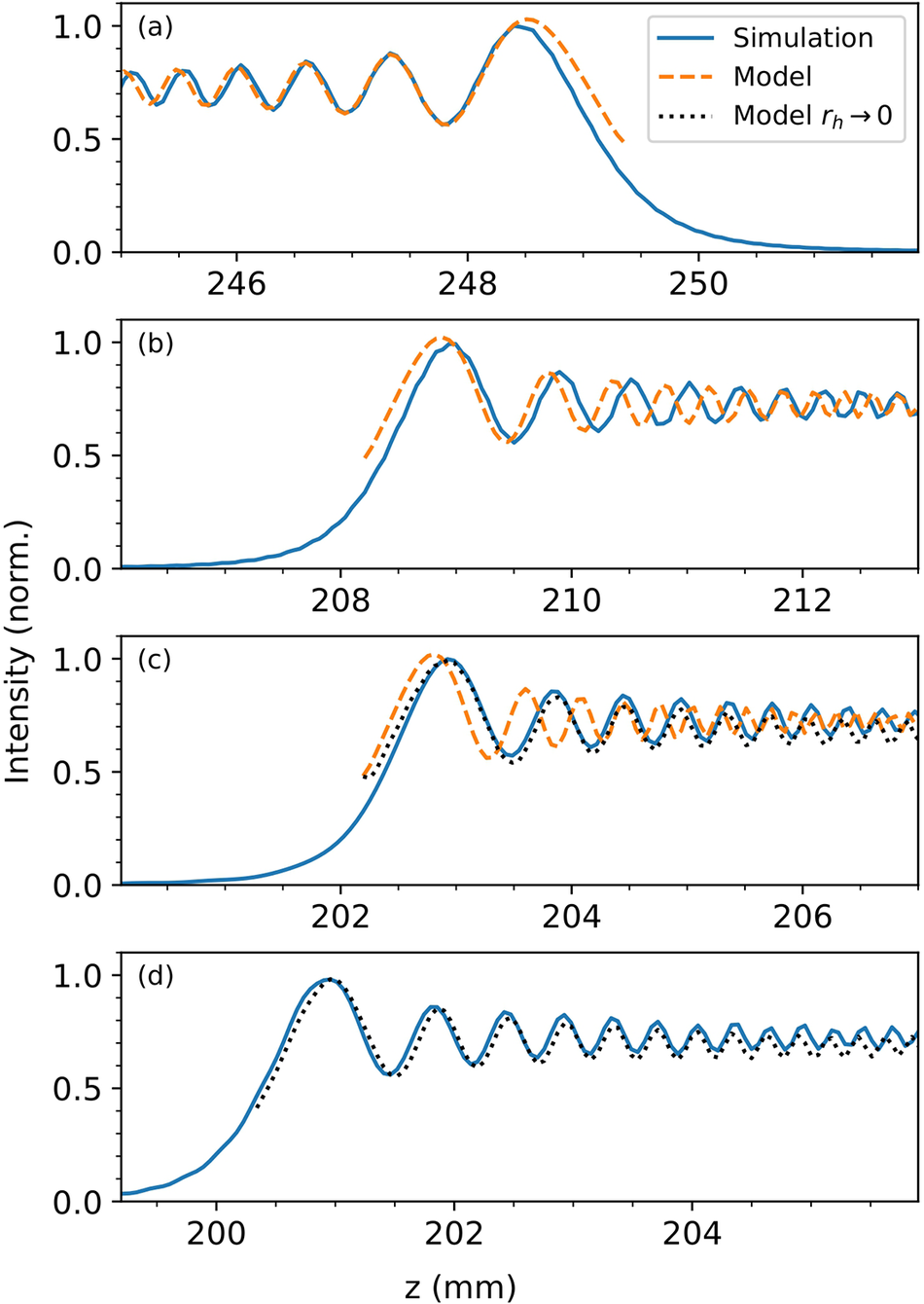
Figure 1 shows the intensity along the optical axis at the end (Figure 1(a)) and at the beginning (Figure 1(b)) of the focal line for a central hole radius ${r}_\mathrm{h}=20$ mm. The agreement between the intensity predicted by Equation (5) (orange curves) and the exact numerical result (blue curves) is excellent at the end of the focal line and fair at the beginning. This agreement degrades as the hole radius ${r}_\mathrm{h}$ decreases, as illustrated in Figure 1(c). Without a central hole, $\Psi$ varies too slowly for the stationary-phase approximation to hold, and the model breaks down.

Figure 1

Intensity along the optical axis at the end (a) and at the beginning (b)–(d) of the focal line for a hole radius of ${r}_\mathrm{h}=20$ mm (b), ${r}_\mathrm{h}=10$ mm (c) and ${r}_\mathrm{h}=0$ mm (d). The blue curves were computed with Axiprop, while the orange curves were obtained using Equation (5), and the green curves were obtained using Equation (9).

Figure 1. Long description

A multi-panel line graph with four vertically stacked panels labeled a, b, c, and d. The y-axis for all panels is Intensity (norm.) ranging from 0.0 to 1.0. The x-axis is z in millimeters.

* Panel a: Shows the end of the focal line. The x-axis ranges from 245 to 251. A solid blue Simulation curve and a dashed orange Model curve show high-frequency oscillations that peak near 248.5 before dropping to zero.

* Panel b: Hole radius r sub h = 20 mm. The x-axis ranges from 206 to 213. The curves show a sharp rise from zero starting at 207, reaching a primary peak at 209, followed by sustained oscillations around an intensity of 0.7.

* Panel c: Hole radius r sub h = 10 mm. The x-axis ranges from 201 to 207. Similar to panel b, the intensity rises sharply at 202, peaks at 203, and continues with oscillations. A third dotted black curve (Model r sub h approaches 0) is introduced, closely following the blue simulation curve, while the orange model begins to deviate from the blue simulation curve.

* Panel d: Hole radius r sub h = 0 mm. The x-axis ranges from 199 to 205. The intensity rises at 200 and peaks at 201. The solid blue simulation curve and the dotted black model curve are nearly perfectly aligned, showing regular oscillations that gradually decrease in amplitude as z increases.

Mathematically, this occurs because $\alpha {a}^2$ in Equation (3) becomes too small to satisfy the equation as ${r}_\mathrm{h}\to 0$ . In this scenario, a more accurate approximation can be obtained by directly expanding $\Psi (r)$ around $r=0$ in Equation (1). In the case of a constant-intensity line, and for $\delta \ll {f}_0$ , the radial phase is as follows^[ Reference Smartsev, Caizergues, Oubrerie, Gautier, Goddet, Tafzi, Phuoc, Malka and Thaury ^{10 ]}:

(7) $$\begin{align}\Psi (r)=-{\alpha}_0{r}^2\left(2{r}_\mathrm{s}^2(z)-{r}^2+\mathcal{O}\left({r}^4/{R}^2\right)\right),\end{align}$$

with ${\alpha}_0=\delta k/4{f}_0^2{R}^2$ . Applying this expression in Equation (1), and introducing the change of variables $u={r}^2$ , leads to the following:

(8) $$\begin{align}E\left(0,z\right)=-i\frac{k}{2z}{E}_0{e}^{ikz+i\Psi \left({r}_\mathrm{s}\right)}{\int}_{\!\!\!\!r_\mathrm{h}^2}^{R^2}{e}^{i{\alpha}_0{\left(u-{r}_\mathrm{s}^2\right)}^2} \mathrm{d}u.\end{align}$$

Using the approximation of Equation (3), this yields the following:

(9) $$\begin{align}E(z)\underset{r_\mathrm{s}\to {r}_\mathrm{h}}{\approx}\frac{A}{2}\left({i e}^{i\pi /4}\sqrt{\frac{2\pi }{\alpha_0}}+\frac{e^{i{\alpha}_0{\left({r}_\mathrm{h}^2-{r}_\mathrm{s}^2\right)}^2}}{\alpha_0\left({r}_\mathrm{h}^2-{r}_\mathrm{s}^2\right)}\right).\end{align}$$

Equation (9) describes an intensity profile that exhibits oscillations similar to those of the stationary-phase model, but with a lower frequency and closer agreement with simulations as ${r}_\mathrm{h}\to 0$ , as shown in Figures 1(c) and 1(d).

2.2 Polychromatic regime

For ultra-short laser pulses, the electric field is also affected by the spectral bandwidth $\Delta k$ , which induces a gradual loss of contrast in the axial intensity oscillations. This effect can be interpreted as a longitudinal dephasing between spectral components. At the beginning of the line, the oscillatory phase term is given by Equation (9):

(10) $$\begin{align}\phi \left({r}_\mathrm{s},k\right)=\frac{\delta k}{4{f}_0^2{R}^2}{\left({r}_\mathrm{h}^2-{r}_\mathrm{s}^2\right)}^2.\end{align}$$

The decoherence length along the optical axis can be estimated by requiring that the phase difference accumulated over the bandwidth satisfies $\Delta \phi \sim \pi$ , which defines a characteristic propagation length ${L}_{z,\mathrm{c}}$ . Using this expression for ${r}_\mathrm{h}=0$ alongside the geometric relation between ${r}_\mathrm{s}$ and $z$ , we obtain the scaling law:

(11) $$\begin{align}{L}_{z,\mathrm{c}}^0=\frac{f}{R}{\left(4\pi \frac{\delta }{\Delta k}\right)}^{1/2}.\end{align}$$

A similar analysis can be performed in the limit ${r}_\mathrm{h}\to R$ , for which Equation (5) leads to the following:

(12) $$\begin{align}\phi \left({r}_\mathrm{s},k\right)=\frac{{\left({r}_\mathrm{h}-{r}_\mathrm{s}\right)}^2}{2}{\Psi^{{\prime}{\prime}}}\left({r}_\mathrm{s},k\right).\end{align}$$

Substituting the explicit dependence of ${\Psi^{{\prime}{\prime}}}\left({r}_\mathrm{s},k\right)$ given by Equation (7) yields a quadratic equation:

(13) $$\begin{align}{r}_\mathrm{s}^2-{Rr}_\mathrm{s}+{f}_0R\sqrt{\frac{2\pi }{3\delta \Delta k}}=0.\end{align}$$

In the regime of strong spectral decoherence, the constant term remains small compared to ${R}^2$ , and using the geometric relation between ${r}_\mathrm{s}$ and $z$ , one obtains the scaling law:

(14) $$\begin{align}{L}_{z,\mathrm{c}}^R=\frac{f}{R}{\left(\frac{8\pi }{3}\frac{\delta }{\Delta k}\right)}^{1/2}.\end{align}$$

We observe that Equations (11) and (14) share the same scaling with respect to the axiparabola parameters and the spectral bandwidth, differing only by a numerical prefactor of order unity. This indicates that the decoherence length is only weakly dependent on the position along the focal line. Consequently, to leading order, the decoherence length can be approximated as position-independent and written as follows:

(15) $$\begin{align}{L}_{z,\mathrm{c}}\approx 3\frac{f}{R}{\left(\frac{\delta }{\Delta k}\right)}^{1/2}.\end{align}$$

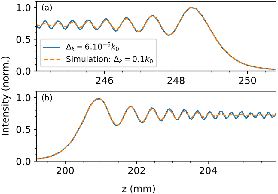
We now validate this scaling law through numerical simulations using the same axiparabola configuration as in the previous section, for both monochromatic and polychromatic beams centered at 800 nm. The spectral width is $\Delta k=0.1{k}_0$ , corresponding to a Fourier-transform-limited pulse duration of $\Delta \tau =15$ fs. The analytical decoherence length is 3 mm, in good agreement with the simulation results shown in Figure 2. A polychromatic pulse therefore induces a progressive damping of the axial intensity oscillations through spectral dephasing, but the effect is insufficient to fully suppress oscillations in practical cases. This decoherence effect strongly contrasts with the case of diffractive or refractive optics, where finite bandwidth manifests primarily as longitudinal chromaticism with much more severe implications^[ Reference Jaroszewicz, Dopazo and Gomez-Reino ^{18 ]}.

Figure 2

Intensity along the optical axis at the end (a) and at the beginning (b) of the focal line. The blue curves were computed for a monochromatic pulse, while the orange curves correspond to a polychromatic laser with a spectral bandwidth $\Delta k=0.1{k}_0$ .

Figure 2. Long description

Two vertically stacked line graphs show normalized intensity on the y-axis ranging from 0.0 to 1.0 against the optical axis z in millimeters on the x-axis.

Panel a at the top displays the end of the focal line with z values from approximately 244 to 251. A solid blue line represents Delta k equals 6 dot 10 super minus 6 k sub 0, and a dashed orange line represents a simulation where Delta k equals 0.1 k sub 0. Both curves show high-frequency oscillations that increase in amplitude as z increases, reaching a final peak of 1.0 at z equals 248.5 before a sharp asymptotic decay toward zero.

Panel b at the bottom displays the beginning of the focal line with z values from 199 to 205. The curves show a smooth rise from zero starting at z equals 199, reaching a primary peak of 1.0 at z equals 201. Following this peak, the intensity exhibits damped oscillations that settle into a steady state of approximately 0.75 as z increases toward 205. The blue and orange curves are nearly identical in both panels, with the polychromatic curve showing a slight damping of the oscillations over a few millimeters while preserving the overall intensity profile.

These results demonstrate that the sharp terminations of the focal line inevitably introduce spurious oscillations, regardless of the beam’s spectral bandwidth. Conversely, this implies that such oscillations can be effectively suppressed by avoiding abrupt intensity transitions, which can be achieved by optimizing either the amplitude or the phase of the incident beam^[ Reference Khonina, Ustinov, Kharitonov, Fomchenkov and Porfirev ^{19 ,} Reference Blum, Puchert, Archer, Jalas, Jolly, Osterhoff, Leemans, Kirchen, Maier and Shalloo ^{20 ]}.

3.1 Model

We first consider the use of an amplitude mask. As demonstrated in Section 2, the oscillations originate from the sharp cutoff of the Fresnel integral. Consequently, we expect to suppress these oscillations by illuminating the axiparabola with a smoother intensity profile^[ Reference Fan, Wang, Wei, Yang, Zhang, Chen, Wu and Cao ^{11 ]}. To validate this approach, we now replace the top-hat profile of the incident laser by a smoother super-Gaussian of the order $n$ , and substitute the sharp central hole with a Gaussian profile:

(16) $$\begin{align}{E}_i(r)={E}_0{e}^{-{\left(r/R\right)}^{2n}}\left\{\begin{array}{ll}{e}^{-{\left(r-{r}_\mathrm{h}\right)}^2/{L}_\mathrm{h}^2}& \mathrm{if}\kern0.22em r\le {r}_\mathrm{h}\\ {}1& \mathrm{if}\kern0.22em r>{r}_\mathrm{h}\end{array}\right.,\end{align}$$

where ${L}_\mathrm{h}$ is the scale length of the Gaussian hole. The electric field along the focal line is then simply obtained by introducing ${E}_i(r)$ into Equation (2), as follows:

(17) $$\begin{align}E(z)=-i\frac{kr_\mathrm{s}}{z}{e}^{ikz+i\Psi \left({r}_\mathrm{s}\right)}{\int}_0^R{\mathrm{d}rE}_i(r){e}^{i{\Psi^{{\prime}{\prime}}}\left({r}_\mathrm{s}\right){\left(r-{r}_\mathrm{s}\right)}^2/2}.\end{align}$$

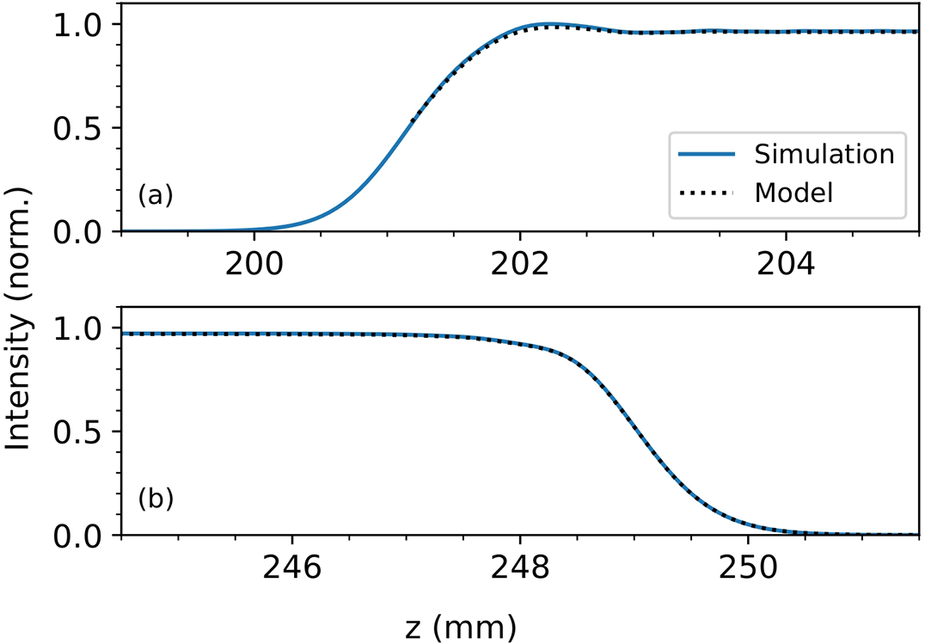
The numerical integration of Equation (17) is plotted in Figure 3, where it is compared to the results of an Axiprop simulation. The parameters used are identical to those in Section 2, except for ${r}_\mathrm{h}=10$ mm, ${L}_\mathrm{h}=4$ mm and $n=100$ . We observe an excellent agreement between the model and the simulations, as well as efficient suppression of the intensity of oscillations.

Figure 3

Intensity along the optical axis at the beginning (a) and at the end (b) of the focal line for a super-Gaussian laser pulse with a Gaussian central hole, as defined by Equation (16).

Figure 3. Long description

A two-panel line graph with a shared y-axis labeled Intensity norm. and a shared x-axis labeled z in m m. Both panels feature a solid blue line for Simulation and a black dotted line for Model.

Panel a shows the beginning of the focal line. The x-axis ranges from 199 to 205. The data starts at zero intensity, begins a sigmoid-like rise around z equals 200, reaches a peak intensity of 1.0 at z equals 202, and then stabilizes with minor oscillations around 0.95. The Simulation and Model lines are nearly perfectly overlapped.

Panel b shows the end of the focal line. The x-axis ranges from 245 to 251. The data starts at a plateau of 1.0 intensity, remains flat until z equals 248, then undergoes a steep sigmoid-like descent, reaching zero intensity by z equals 250. The Simulation and Model lines show high agreement throughout the transition.

3.2 Experiment

To verify the theoretical predictions, we performed an experiment using a He–Ne laser with a central wavelength of $\lambda =633$ nm. The top-hat beam was directed onto an axiparabola designed to produce a constant-intensity line, characterized by ${f}_0=200$ mm and $\delta =30$ mm, for an input beam diameter of ${R}_\mathrm{m}=50.8$ mm. Amplitude modulation was applied using a Holoeye LC2012 spatial light modulator (SLM) with a resolution of 1024 $\times$ 768 pixels and a pixel pitch of 36 $\unicode{x3bc}\mathrm{m}$ . The Gaussian beam delivered by the He–Ne laser was expanded before the SLM to achieve a beam waist of 40 mm, and then to an aperture diameter of 27.6 mm to match the active area of the modulator. After the SLM, the beam was expanded by a factor of 2.5, resulting in a truncated Gaussian beam with a waist of approximately 100 mm and an aperture of 69 mm on the axiparabola surface. The focal region was imaged onto a complementary metal–oxide–semiconductor (CMOS) camera through a microscope objective. The imaging system (microscope and camera) was mounted on a motorized translation stage, allowing the measurement of the axial evolution of the on-axis intensity distribution.

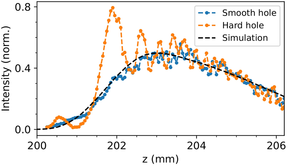
Figure 4 presents the recorded on-axis intensity profiles for both a sharp and a smooth hole, as defined by Equation (16), for ${r}_\mathrm{h}=11.6$ mm and ${r}_\mathrm{h}=16.75$ mm, respectively, with ${L}_\mathrm{h}=5.15$ mm. Each data point corresponds to the average of 10 images acquired with an exposure time of 200 ms. Similar to Figures 1 and 3, pronounced oscillations are observed when using a sharp hole, while they are well suppressed with the Gaussian hole. A noticeable difference is observed in the intensity profile: instead of reaching the expected plateau after the hole, the intensity decreases. This behavior can be attributed to a trefoil aberration generated by the axiparabola, which distorts the focal intensity distribution. Introducing a trefoil aberration ${\Phi}_{\mathrm{trefoil}}\left(r,\theta \right)=2\pi \kern0.1em {a}_3\kern0.1em \cos \left(3\theta {\left(\frac{r}{R}\right)}^3\right)$ in Equation (1) modifies the amplitude distribution by the following factor:

(18) $$\begin{align}{J}_0\left(2\pi {a}_3{\left(\frac{z-{f}_0}{\delta}\right)}^{3/2}\right),\end{align}$$

Figure 4

Experimental on-axis intensity profiles obtained with a sharp hole (orange) and a Gaussian hole (blue) with ${r}_\mathrm{h}=11.6$ mm and ${r}_\mathrm{h}=16.75$ mm, respectively. The theoretical prediction from simulation is shown as dashed lines.

Figure 4. Long description

The x-axis represents z in m m, ranging from 200 to 206. The y-axis represents Intensity (norm.) ranging from 0.0 to 0.8.

* The Simulation (black dashed line) shows a smooth, broad bell-shaped curve peaking at approximately 0.5 intensity around z equals 203 m m.

* The Smooth hole (blue dashed line with circular markers) follows the simulation trend closely but with high-frequency noise, fluctuating around the theoretical curve.

* The Hard hole (orange dashed line with circular markers) exhibits high-amplitude oscillations. It features a sharp primary peak reaching 0.8 intensity at z equals 201.8 m m, followed by three subsequent smaller peaks at z equals 202.6, 203.4, and 203.8 m m before converging toward the other data sets near z equals 205 m m.

A legend in the top right corner identifies the blue line as Smooth hole, the orange line as Hard hole, and the black dashed line as Simulation.

where ${a}_3$ is the trefoil coefficient expressed in units of the wave number. The simulated curve shown in Figure 4 implements the amplitude modulation described by Equation (18), resulting in good agreement with the experimental data, with a measured trefoil coefficient of ${a}_3=2.2$ . Importantly, this reduction in intensity could be mitigated by using deformable mirrors to correct for the aberration. While demonstrated here with a monochromatic low-power laser, this approach could be transposed to high-fluence systems using high-damage-threshold SLMs^[ Reference Ramousse, Chériaux, Claudet and Jullien ^{21 –} Reference Monvoisin, Mesplede, Rouzaud, Montant, Lamaignère, Claudet, Chériaux, Forget and Jullien ^{23 ]}.

4.1 Model

We showed in Section 3 that oscillations can be efficiently suppressed by applying amplitude modulation on the incoming beam. Although oscillations originating from the outer edge of the beam are often naturally suppressed, since real beams are naturally super-Gaussian, the suppression of oscillations originating from the central part of the beam is more challenging. Indeed, producing a smooth intensity dip at the center of the incoming beam would require absorbing a significant fraction of the incident energy, which could damage the optical components used for that purpose. Suppressing these oscillations by acting only on the phase of the beam, through the use of a focusing optic, an SLM or a phase mask, would therefore be highly desirable. In this section, we investigate the conditions under which such phase-based suppression can be achieved.

Different strategies can be adopted to avoid oscillations at the beginning of the focal line. Since these oscillations originate from abrupt variations in the desired intensity profile, one approach is to define a longitudinal intensity distribution that smoothly rises from low values before transitioning into a constant plateau, similar to what can be obtained through amplitude shaping, and then compute the phase that generates this profile. An alternative approach would consist of using an iterative algorithm to determine the optimal phase under given constraints^[ Reference Čižmár and Dholakia ^{24 ,} Reference Li, Yu, Peng, Yang, Yao, Zhang and Ye ^{25 ]}.

Here, we adopt the simplest approach and start directly from a given phase profile, which we modify to suppress the oscillations. As discussed in Section 2, oscillations arise when the second derivative of the radial beam phase before focus is too small to blur interferences between different regions of the beam. Consequently, oscillations can be mitigated by artificially increasing ${\Phi^{{\prime}{\prime}}}(r)$ for any $r<{r}_0$ , where ${r}_0$ is an arbitrary radius. For example, one can simply replace the beam phase for $r<{r}_0$ with the following:

(19) $$\begin{align}\Phi (r)=\Phi \left({r}_0\right)+{\Phi}^{\prime}\left({r}_0\right)\kern0.1em \left(r-{r}_0\right)+\frac{1}{2}{\Phi^{{\prime}{\prime}}}\left({r}_0\right)\kern0.1em {\left(r-{r}_0\right)}^2,\end{align}$$

so that ${\Phi^{{\prime}{\prime}}}(r)$ remains constant for $r<{r}_0$ .

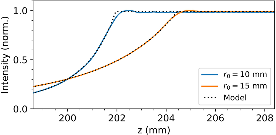
This approach was validated through two Axiprop simulations performed for ${r}_0=10$ mm and ${r}_0=15$ mm, using the same axiparabola parameters as in Sections 2 and 3.1. As shown in Figure 5, oscillations are strongly damped for ${r}_0=10$ mm, similar to amplitude shaping, and almost completely suppressed for ${r}_0=15$ mm. Since Equation (6) is satisfied, the on-axis intensity can be computed directly from Equation (4). The resulting profiles, plotted in Figure 5, show excellent agreement with the numerical simulations. Furthermore, the intensity evolution within the rising ramp can be obtained analytically by deriving ${r}_\mathrm{s}(z)$ for the phase defined in Equation (19), leading to the following:

$$\begin{align*}I(z)\propto \frac{z}{{\left({k}_0-z{\Phi^{{\prime}{\prime}}}\left({r}_0\right)\right)}^3}.\end{align*}$$

Figure 5

On-axis intensity profiles obtained from Axiprop simulations using the modified phase approach. Profiles are shown for ${r}_0=10$ mm (blue line) and ${r}_0=15$ mm (orange line). The dotted lines correspond to the profiles obtained from Equation (4).

Figure 5. Long description

The x-axis represents z in millimeters, ranging from 198.5 to 208.5. The y-axis represents Intensity (norm.) ranging from 0.0 to 1.0.

Two data series are plotted:

* A blue solid line for r sub 0 = 10 mm starts at an intensity of approximately 0.2 at z = 198.5, rises steeply in a sigmoidal curve, and reaches a plateau of 1.0 at approximately z = 202.

* An orange solid line for r sub 0 = 15 mm starts at approximately 0.25, rises with a shallower slope, and reaches the 1.0 plateau later, at approximately z = 205.

Black dotted lines representing the Model closely track both solid lines. For the r sub 0 = 10 mm case, the model shows a sharp corner at the transition to the plateau, while the simulation (blue line) shows a slight overshoot and oscillation before stabilizing. A similar but less pronounced behavior is seen for the r sub 0 = 15 mm case near z = 205. Both profiles remain stable at an intensity of 1.0 from their respective saturation points through z = 208.5.

This expression shows that the intensity profile exhibits a long leading edge, vanishing only as $z$ approaches zero. In practice, the shape and extent of this ramp could be readily adjusted to meet the requirements of a specific experiment by employing a more elaborate phase profile, potentially designed using iterative algorithms^[ Reference Čižmár and Dholakia ^{24 ,} Reference Li, Yu, Peng, Yang, Yao, Zhang and Ye ^{25 ]}.

More generally, this phase-engineering approach provides a direct method for designing oscillation-free axiparabola profiles, which can be implemented experimentally using custom-shaped mirrors alone. Alternatively, the same profiles can be synthesized by combining a standard axiparabola with a phase-modulating element, such as a deformable mirror^[ Reference Blum, Puchert, Archer, Jalas, Jolly, Osterhoff, Leemans, Kirchen, Maier and Shalloo ^{20 ]}, a phase plate or a high-damage-threshold SLM.

4.2 Experiment

As in Section 3.2 for the amplitude-based approach, we now turn to an experimental investigation to validate the predictions of the phase-based method. The experimental configuration is identical to the previous setup, except for one important modification: because the phase delay achievable with a single SLM is limited, we employed two SLMs in combination. In addition, we used a laser diode with a central wavelength of $\lambda =405$ nm.

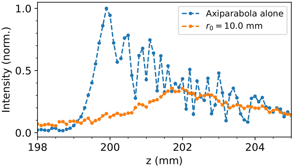
Figure 6 shows the recorded intensity profiles for the unmodulated beam and for the beam shaped with a phase modulation of ${r}_0=10$ mm. Each data point corresponds to the average of 20 images acquired with an exposure time of 100 ms. We observe that the oscillations are strongly damped, with a long rising ramp, in good agreement with the simulations.

Figure 6

Experimental on-axis intensity profiles obtained without modulation (blue) and with a phase modulation (orange) with ${r}_\mathrm{h}=10$ mm.

Figure 6. Long description

The x-axis represents z in millimeters, ranging from 198 to 205. The y-axis represents normalized intensity, ranging from 0.0 to 1.0.

* The blue dashed line with circular markers, labeled Axiparabola alone, shows a sharp rise starting at z equals 199, reaching a primary peak of 1.0 at z equals 200. Following this peak, the intensity exhibits high-frequency oscillations with a general downward trend, fluctuating between 0.1 and 0.8 as z increases toward 205.

* The orange dashed line with circular markers, labeled r sub 0 equals 10.0 mm, shows a much flatter profile. It maintains a low intensity near 0.1 until z equals 200, then gradually increases to a broad, stable plateau around 0.3 between z equals 201.5 and 203.5, before slightly tapering off toward 205.

The comparison shows that the phase modulation significantly suppresses the peak intensity while smoothing the axial distribution.

A notable difference, however, is the decrease in intensity along the line, whereas a nearly constant intensity was expected. This discrepancy likely results from the use of two SLMs, which introduces noticeable aberrations, further aggravated by one device’s partial pre-existing deterioration.

5.1 Resolution limit

In the previous sections, we demonstrated the production of extended focal lines free of unwanted modulations. However, it may sometimes be desirable to produce controlled modulations^[ Reference Khonina, Ustinov, Kharitonov, Fomchenkov and Porfirev ^{19 ]}. From Section 2, we know that sharp transitions lead to unwanted oscillations; therefore, we cannot generate structures of arbitrarily small size. To estimate the achievable resolution, we can use Equation (3) with $b=\infty$ and $a={L}_\mathrm{r}$ , where ${L}_\mathrm{r}$ is the scale length of the radial modulation. To avoid spurious interferences, we require ${L}_\mathrm{r}$ to be large enough to ensure that $1/\left(2\alpha a\right)\ll {\left(\pi /\alpha \right)}^{1/2}$ . By substituting $\alpha$ with ${\Psi^{{\prime}{\prime}}}/2$ , we obtain the following condition:

(20) $$\begin{align}{L}_\mathrm{r}\gg {\left(2\pi {\Psi^{{\prime}{\prime}}}\right)}^{-1/2}.\end{align}$$

Substituting the explicit dependence of ${\Psi^{{\prime}{\prime}}}\left({r}_\mathrm{s},k\right)$ given by Equation (7) into Equation (20), we derive the following condition:

(21) $$\begin{align}{L}_\mathrm{r}\gg {L}_{\mathrm{r}_0}=\frac{R}{r}\frac{f_0}{{\left(6\pi k\delta \right)}^{1/2}}.\end{align}$$

It is more informative to translate this radial scale length into an achievable longitudinal resolution along the focal line. For a constant-intensity line, this translation is straightforward, as we have the relation $z={f}_0+\delta {r}^2/{R}^2$ . This leads to a longitudinal resolution:

(22) $$\begin{align}{L}_z\gg \frac{2\delta {rL}_{\mathrm{r}_0}}{R^2}=\frac{f}{R}{\left(\frac{2\delta }{3\pi k}\right)}^{1/2}.\end{align}$$

Interestingly, the achievable resolution is independent of the position along the focal line and depends only on the numerical aperture and the focal depth. While derived for the constant-intensity axiparabola considered here, this approach can be extended to other intensity profiles by adapting it to the specific configuration.

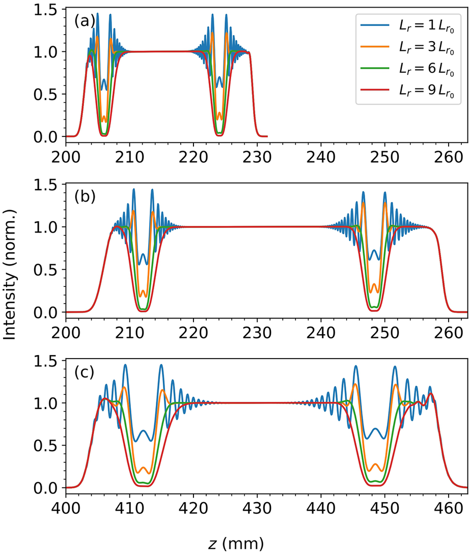
To validate this estimate, we performed a set of Axiprop simulations. We considered a radial intensity profile featuring two Gaussian holes located at ${r}_1=0.45R$ and ${r}_2=0.9R$ , described by ${E}_i(r)={E}_{i0}(r)-{E}_0\exp \left(-{\left(r-{r}_i\right)}^2/{L}_{\mathrm{r}i}^2\right)$ where $i\in \left\{1,2\right\}$ , ${E}_{i0}(r)$ is the radial profile without a hole and ${L}_{\mathrm{r}i}={L}_\mathrm{r}\left({r}_i\right)$ . Figure 7 presents the simulation results for $R=50$ mm, ${f}_0\in \left\{\mathrm{200,400}\right\}$ mm, $\delta \in \left\{30,60\right\}$ mm and various values of ${L}_\mathrm{r}\in \left\{\mathrm{1,3,6,9}\right\}{L}_{\mathrm{r}_0}$ .

Figure 7

On-axis intensity profiles obtained from simulations for different axiparabola parameters: (a) ${f}_0=200$ mm and $\delta =30$ mm; (b) ${f}_0=200$ mm and $\delta =60$ mm; (c) ${f}_0=400$ mm and $\delta =60$ mm. The curves correspond to different values of ${L}_\mathrm{r}\in \left\{\mathrm{1,3,6,9}\right\}{L}_{\mathrm{r}_0}$ .

Figure 7. Long description

A three-panel vertical stack of line graphs labeled a, b, and c.

Common Axes: The vertical y-axis represents Intensity (norm.) ranging from 0.0 to 1.5. The horizontal x-axis represents z in millimeters.

Legend: Each panel contains four curves: blue (L sub r = 1 L sub r sub 0), orange (L sub r = 3 L sub r sub 0), green (L sub r = 6 L sub r sub 0), and red (L sub r = 9 L sub r sub 0).

Panel a: The x-axis ranges from 200 to 260. The curves show a flat plateau at intensity 1.0 between z = 210 and 220. On either side of this plateau, the curves exhibit sharp oscillations and deep troughs. The blue curve has the highest oscillation peaks and deepest troughs, while the red curve is the smoothest with the shallowest troughs.

Panel b: The x-axis ranges from 200 to 260. The central plateau at intensity 1.0 is wider, extending from z = 218 to 242. Similar to panel a, the blue curve shows the most extreme oscillations at the edges of the plateau, and the red curve shows the least.

Panel c: The x-axis ranges from 400 to 460. The central plateau at intensity 1.0 is narrower, located between z = 420 and 440. The oscillatory regions at the boundaries are broader than in the previous panels. The blue curve reaches peaks near 1.5, while the red curve remains closest to the 1.0 baseline with minimal dipping.

We observe that the hole depth is reduced and that fringes begin to appear for ${L}_\mathrm{r}\le 6{L}_{\mathrm{r}_0}$ . In addition, we find that ${L}_z$ increases linearly with ${f}_0$ and scales as ${\delta}^{-1/2}$ while remaining independent of the longitudinal position, as expected. Thus, Figure 7 validates the scaling law given by Equation (22). It also provides an order-of-magnitude estimate for the achievable longitudinal resolution:

(23) $$\begin{align}{L}_z\approx 2.8\frac{f_0}{R}{\left(\frac{\delta }{k}\right)}^{1/2}.\end{align}$$

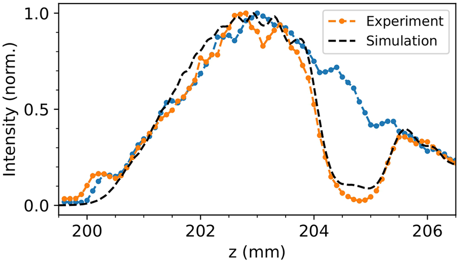
We now turn to an experimental validation of this theoretical resolution, using the same setup as in Section 3.2. Figure 8 shows the recorded intensity profile for a radial profile featuring a smooth central hole, as described in Section 3.2, followed by a Gaussian ring with parameters ${r}_1=20.3\ \mathrm{mm}$ and ${L}_1=1.82\ \mathrm{mm}$ . Each data point corresponds to the average of 10 images acquired with an exposure time of 200 ms, and a moving average with a window size of three data points was applied to smooth the profile.

Figure 8

Experimental on-axis intensity profiles obtained with a smooth central hole with (orange) and without (blue) a Gaussian ring defined by ${L}_1=1.82\ \mathrm{mm}$ and ${r}_1=20.3\ \mathrm{mm}$ . The theoretical prediction from simulations is shown in black.

Figure 8. Long description

The x-axis represents z in millimeters, ranging from 199.5 to 206.5. The y-axis represents normalized intensity from 0.0 to 1.0.

* The data consists of three main profiles: an orange dotted line (Experiment with Gaussian ring hole), a blue dotted line (Experiment without Gaussian ring hole), and black dashed lines (Theoretical simulations).

* From 200 to 202 millimeters, all curves show a steady linear increase with minor fluctuations.

* Between 202 and 204 millimeters, the profiles reach a broad peak near 1.0 intensity. The orange experimental line and its corresponding black dashed simulation show a sharp drop-off starting at 204 millimeters, reaching a trough near 0.1 intensity at 205 millimeters.

* The blue experimental line maintains a higher intensity plateau between 204 and 205 millimeters compared to the orange line, before converging with the other data sets.

* All curves show a secondary smaller peak around 205.5 millimeters before trending downward toward the end of the measured range.

As expected, a hole is observed in the plateau of the axiparabola. By fitting the profile with a Gaussian function, we find that the hole has a width of $0.5\ \mathrm{mm}$ , which is of the same order of magnitude as the longitudinal resolution ${L}_z\approx 0.67\ \mathrm{mm}$ given by Equation (23). The theoretical curve shown in the figure indicates that the experimentally measured contrast is even slightly better than expected, likely related to optical aberrations. In principle, similar longitudinal modulations could be achieved using phase-only modulation^[ Reference Khonina, Ustinov, Kharitonov, Fomchenkov and Porfirev ^{19 ]}.

For a polychromatic laser, the amplitude modulation is affected by spectral decoherence. It is therefore instructive to compare the axial resolution length ${L}_z$ with the decoherence length defined in Equation (15), leading to the dimensionless ratio:

(24) $$\begin{align}\frac{L_z}{L_{z,\mathrm{c}}}\approx {\left(\frac{\Delta k}{k}\right)}^{1/2}.\end{align}$$

This ratio indicates that the decoherence length always remains larger than the longitudinal resolution, implying that increasing the spectral bandwidth does not significantly modify the resolution, but rather only enhances oscillation damping.

5.2 Oscillating profile

Among the various forms of longitudinal intensity modulation, sinusoidal modulations have already attracted significant interest. They have been identified as a promising approach to boost X-ray emission in laser–plasma accelerators^[ Reference Tomkus, Girdauskas, Dudutis, Gečys, Stankevič, Račiukaitis, González, Guénot, Svensson, Persson and Lundh ^{16 ]}, as well as to increase the electron energy through quasi-phase matching in laser-wakefield acceleration^[ Reference Yoon, Palastro and Milchberg ^{15 ,} Reference York, Milchberg, Palastro and Antonsen ^{26 ]}. For the first application, the desired spatial period is of hundreds of micrometers, while the second application is linked to the dephasing length going from hundreds of micrometers to few centimeters. An efficient way to generate such longitudinal modulations is to imprint a radial intensity modulation on the beam prior to the optics that produce the quasi-Bessel beam^[ Reference Layer, York, Antonsen, Varma, Chen, Leng and Milchberg ^{27 ]}. Here, we build on this idea to determine, both numerically and experimentally, the achievable spatial frequencies.

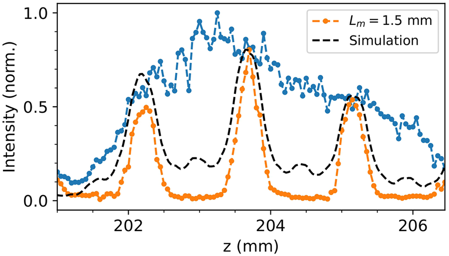
As a preliminary step, we scanned several oscillation periods and found that well-contrasted oscillations persist for periods as short as ${L}_\mathrm{m}=1.5\kern0.1em \mathrm{mm}$ , where ${L}_\mathrm{m}$ denotes the period of the sinusoidal modulations we aim to achieve. This value is consistent with the longitudinal resolution ${L}_z$ determined in Section 5.1. The experimental on-axis intensity profiles and the corresponding simulated curve for this minimum period are shown in Figure 9. While clearly resolved, the modulation, originally designed to be sinusoidal, exhibits sharper peaks and flatter troughs. Interestingly, the contrast of the experimentally observed oscillations is higher than that predicted by the simulations, in agreement with the trend already observed in Figure 8.

Figure 9

Experimental on-axis intensity profiles obtained with a smooth central hole, with (orange) and without (blue) sinusoidal modulation of spatial period ${L}_\mathrm{m}=1.5\kern0.1em \mathrm{mm}$ . The theoretical prediction from simulations is shown in black.

Figure 9. Long description

The line graph plots Intensity (norm.) on the y-axis from 0.0 to 1.0 against z (m m) on the x-axis from approximately 201 to 206.5.

* The blue data series represents the profile without modulation, showing a broad, noisy plateau of high intensity between z = 202 and 205, peaking near 1.0 at z = 203.5.

* The orange data series represents the profile with sinusoidal modulation (L sub m = 1.5 m m). It shows three distinct, sharp peaks at approximately z = 202.2, 203.7, and 205.2. The central peak is the highest, reaching nearly 0.8.

* Black dashed lines represent the theoretical simulations. For the modulated case, the simulation closely follows the three-peak structure of the orange data. For the non-modulated case, the simulation shows a smoother, broader curve that underlies the noisy blue experimental data.

* A legend in the top right identifies the orange dashed line with a dot as L sub m = 1.5 m m and the black dashed line as Simulation.

These results demonstrate that millimeter-scale oscillations can be achieved with high contrast. Regarding applications, such millimeter-scale modulation appears too coarse for X-ray-emission enhancement schemes, which typically require sub-millimeter periods. However, it may be suited to quasi-phase matching in laser-wakefield accelerators.

5.3 Segmented optics

In the previous sections, we saw that interference sets a fundamental limit on intensity-shaping resolution. Here, we show that segmented optics can overcome this limit, allowing the creation of intensity profiles that are otherwise inaccessible. By dividing the optic into two or more concentric segments, with a temporal delay between adjacent segments at least equal to the pulse duration, temporal overlap between their contributions is avoided. This suppresses interference at the transitions, enabling steep variations without spurious oscillations.

Even with segmentation, the ultimate feature size remains constrained by diffraction and by the numerical aperture of each optic segment. These factors impose a fundamental resolution limit on the achievable longitudinal intensity structure. Considering, for example, a ring of light with inner radius ${R}_1$ and radial thickness $\sigma$ , uniformly illuminated and focused by a parabolic optic of focal length ${f}_1$ , the resulting on-axis intensity, obtained using Equation (1), is as follows:

(25) $$\begin{align}I(z)\propto {\operatorname{sinc}}^2\left(\frac{k_0}{4}\left({\sigma}^2+2{R}_1\kern0.1em \sigma \right)\left(\frac{f_1-z}{f_1^2}\right)\right),\end{align}$$

leading to a standard deviation in the main lobe:

(26) $$\begin{align}{\sigma}_z\approx \frac{2.1{\lambda}_0{f}_1^2}{\pi \left({\sigma}^2+2{R}_1\kern0.1em \sigma \right)}=\frac{2.1{\lambda}_0{f}_1^2}{S}.\end{align}$$

This shows that the resolution depends only on the illuminated area $S$ and the focal length ${f}_1$ , and is independent of the ring’s radial position ${R}_1$ . For a sufficiently large illuminated area, the resolution can thus be reduced to well below the millimeter scale.

We illustrate this approach by generating a flat-top intensity profile featuring a sharp spike, whose width cannot be achieved without segmented optics. This configuration uses an optic with two segments: a central parabolic region with ${f}_1=205\kern0.22em \mathrm{mm}$ and ${R}_1=12\kern0.22em \mathrm{mm}$ , and an outer axiparabola defined by ${f}_0=200\kern0.22em \mathrm{mm}$ , $\delta =30\kern0.22em \mathrm{mm}$ and $R=50\kern0.22em \mathrm{mm}$ . In addition, amplitude modulation was applied to mitigate residual oscillations, with parameters ${R}_{\mathrm{hole}}=18\kern0.22em \mathrm{mm}$ and ${L}_{\mathrm{hole}}=4\kern0.22em \mathrm{mm}$ .

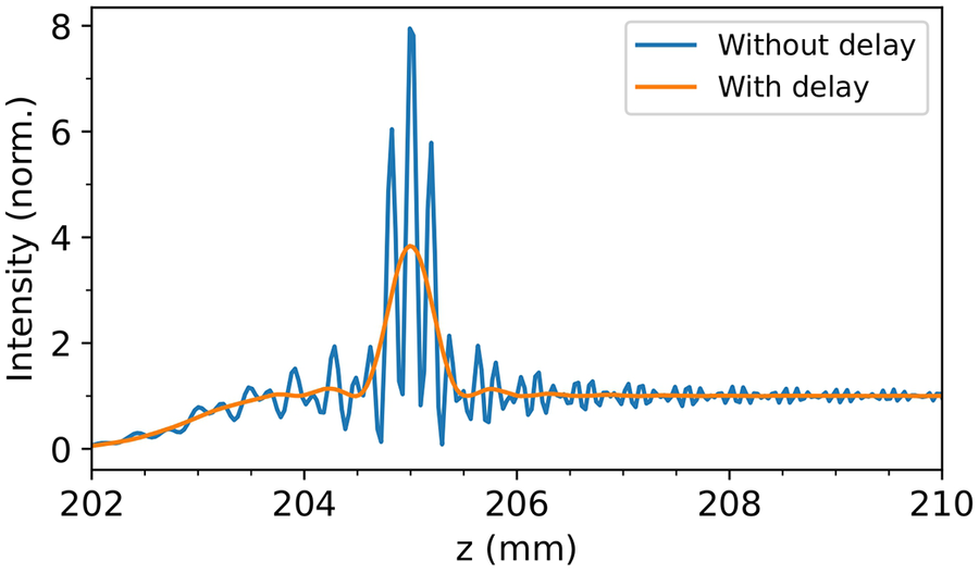
The resulting on-axis intensity profiles are shown in Figure 10. Without delay, the segmented design exhibits strong interference between contributions from different regions of the optic. Introducing a temporal delay between segments eliminates this overlap, achievable in practice through a longitudinal gap between the segments, and enables the formation of a sharp leading spike with a width of 0.16 mm – significantly smaller than both the experimental width and the theoretical resolution limit in Section 5.1.

Figure 10

On-axis intensity profile obtained from simulations for a segmented axiparabola with and without radial delay.

Figure 10. Long description

The line graph plots Intensity (norm.) on the y-axis from 0 to 8 against z (m m) on the x-axis from 202 to 210.

* The x-axis represents the longitudinal position z in millimeters.

* The y-axis represents the normalized intensity.

* A blue line labeled Without delay shows a highly oscillatory pattern. It begins near 0 at z = 202, gradually increases with small oscillations until z = 204.5, where it enters a region of rapid, high-amplitude oscillations. The primary peak reaches a maximum intensity of approximately 8 at z = 205. Following this peak, the oscillations continue with decreasing amplitude until stabilizing near an intensity of 1 beyond z = 207.

* An orange line labeled With delay shows a much smoother, broader curve. It follows the general trend of the blue line but lacks the rapid oscillations. It rises to a single, smooth peak of approximately 4 at z = 205 and then levels off to an intensity of 1, matching the baseline of the blue line in the far-field region.

This demonstrates that segmentation, combined with appropriate temporal delay, enables the generation of complex, high-resolution intensity features that cannot be achieved with a single continuous optic relying solely on amplitude or phase shaping. Such control over the longitudinal intensity profile opens the possibility of applying segmented optics to advanced laser–plasma concepts, including Trojan-horse injection^[ Reference Hidding, Pretzler, Rosenzweig, Königstein, Schiller and Bruhwiler ^{28 ]} and tailored plasma-density shaping for betatron-radiation generation^[ Reference Phuoc, Esarey, Leurent, Cormier-Michel, Geddes, Schroeder, Rousse and Leemans ^{29 ]}.