Propeller wake evolution mechanisms in oblique flow conditions

M. Felli; M. Falchi

doi:10.1017/jfm.2018.232

Propeller wake evolution mechanisms in oblique flow conditions

Published online by Cambridge University Press: 27 April 2018

M. Felli

and

M. Falchi

Show author details

M. Felli*: Affiliation:
INSEAN-CNR, National Research Council, Maritime Research Centre, Via di Vallerano 139, 00128 Roma, Italy
M. Falchi: Affiliation:
INSEAN-CNR, National Research Council, Maritime Research Centre, Via di Vallerano 139, 00128 Roma, Italy
*: †Email address for correspondence: mario.felli@cnr.it

Article contents

Abstract
Introduction
Reference frames and dimensionless groups
Experimental set-up
Test conditions
Results
Summary and conclusions
References

Rights & Permissions

Abstract

In the present study the wake flow past an isolated propeller operating in oblique flow conditions is investigated experimentally. In particular, the investigation concerns a systematic topological comparison of the wake behaviour in axisymmetric and in oblique inflow conditions, for three inclination angles, and is focused on an analysis of the underlying mechanisms of wake evolution and instability. To this end, the experiment has been designed to investigate the dynamics of propeller vortical structures over a wide spatial extent covering the wake region from the propeller disk up to 4.5 diameters in the streamwise direction. Detailed flow measurements have been undertaken by particle image velocimetry (PIV), using a multicamera configuration with three cameras arranged side by side. This allowed simultaneous acquisition of a large flow extent at a spatial resolution adequate to resolve the smallest vortical structures involved in the process of propeller wake instability. The analysis has been based on both phase-locked averaged and instantaneous flow fields. The study extends the knowledge on the subject of propeller wake dynamics, highlighting the major hydrodynamic effects that non-axisymmetric propeller operating conditions exert on the mechanisms of wake evolution, instability and breakdown, such as asymmetric destabilization of the tip vortices on the leeward and windward sides of the wake, and the interference between the tip and the junction vortices, as well as the cause–effect relation between the breakdown of the blade trailing wake and the instability of the tip and hub vortices.

JFM classification

Vortex Flows: Vortex dynamics Vortex Flows: Vortex instability Vortex Flows: Vortex interactions

Information

Type: JFM Papers
Information: Journal of Fluid Mechanics , Volume 845 , 25 June 2018, pp. 520 - 559
DOI: https://doi.org/10.1017/jfm.2018.232 [Opens in a new window]
Copyright: © 2018 Cambridge University Press

1 Introduction

The performances of rotor systems, such as wind turbines and propellers, are strongly affected by the inflow characteristics, which can considerably alter their propulsive efficiency or energy extraction efficiency as well as their structural response and radiated noise. For example, in large wind parks, where interior turbines are exposed to wake flows from the surrounding turbines, the mutual interaction among rotor wakes is crucial for power production, the fatigue lifetime of the rotors and their environmental impact (see, for example, Frandsen & Thøgersen Reference Frandsen and Thøgersen1999; Leung & Yang Reference Leung and Yang2012; Stevens & Meneveau Reference Stevens and Meneveau2014). Analogously, for ship and pusher aeronautic propellers, the unsteady inflow generated by the fuselage or by the ship hull, along with the turbulence ingested by the propeller, produce a subsequent unsteady response of the propulsor which might involve a considerable increase of both the overall noise emission (see, for example, Cumpsty & Lowrie Reference Cumpsty and Lowrie1974; Robison & Peake Reference Robison and Peake2014) and the fatigue stresses on the blades and the shaft (see Carlton Reference Carlton2012). Furthermore, in naval propulsion, environmental motion, such as waves, wind or currents, and manoeuvring operations can lead to a significant lateral flow which can strongly modify the propeller working conditions and affect the dynamic response of the ship, even dramatically in some extreme cases (Vivianiet al. Reference Viviani, Podenzana Bonvino, Mauro, Cerruti, Guadalupi and Menna2007; Atsavapranee et al. Reference Atsavapranee, Miller, Day, Klamo and Fry2010; Dubbioso, Muscari & Di Mascio Reference Dubbioso, Muscari and Di Mascio2013). In this context, one of the crucial elements for the successful design of propellers is to enhance understanding of the mechanism underlying the interaction between the upstream flow and the dynamics of the resulting coherent turbulent structures detached from the blades.

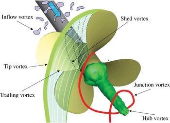
From a theoretical standpoint, the flow behind a rotor is analogous to a rolling wing, which rotates about one tip while advancing, and thus consists of a vortex sheet which is generated by the spanwise gradient of the blade circulation $\unicode[STIX]{x2202}\unicode[STIX]{x1D6E4}/\unicode[STIX]{x2202}r$ and which rolls up into two strong counter-rotating vortices at both the root and tip sections of the blade (see sketch in figure 1).

Figure 1.

Sketch of the vortical systems in the wake of a propeller operating in a non-uniform inflow.

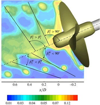
In non-ideal conditions, namely when the rotor operates in a non-uniform or in an oblique flow, the blade circulation is time-dependent (i.e. $\unicode[STIX]{x2202}\unicode[STIX]{x1D6E4}/\unicode[STIX]{x2202}t\neq 0$ ), implying a secondary vortical system is generated, leaving the blade parallel to the trailing edge (see, for example, Di Mascio, Muscari & Dubbioso Reference Di Mascio, Muscari and Dubbioso2015; Micallef & Sant Reference Micallef, Sant, Aissaoui and Tahour2016), so as to locally satisfy the Kutta condition. In this case, blades are exposed to unsteady hydrodynamic loads due to the locally phase-dependent velocity distribution at the leading edge, being the superposition of the variable inflow velocity, the blade velocity and the wake-induced velocity via self-induction effects (Kerwin Reference Kerwin1986; Leishmann Reference Leishmann2006). Behind the rotor, the vortical systems generated by the blades are convected with the local velocity of the flow, including the velocity induced by the wake itself, and undergo a progressive distortion from the basic helix with a highly non-uniform distribution of the hydrodynamic pitch (Jessup Reference Jessup1989). This behaviour is further complicated when the upstream flow interacts strongly with the rotor wake, as typically occurs when a propeller operates in behind conditions (Felli & Di Felice Reference Felli and Di Felice2005), when a helicopter rotor moves in forward flight (Leishmann Reference Leishmann2006) or when the distance between neighbouring turbines within a wind park is not large enough to avoid the wake structures of the upstream rotors impinging on the downstream ones (see, for example, Stevens & Meneveau Reference Stevens and Meneveau2017). In these circumstances, the unsteady hydrodynamic conditions which the blade experiences during a complete rotation when operating in an unsteady and/or in a non-uniform inflow, as well as the interaction between the vortical structures of the wake and the upstream flow, may significantly affect the dynamic evolution of the rotor wake and, in particular, the characteristics and the onset of wake instability.

The study of the wake dynamics of rotor systems has attracted considerable attention in the literature, especially with regard to the mechanisms underlying wake instability. The state of the art indicates that the stability of a rotor wake is a consequence of the mutual interaction among the tip and root vortices with the vortex sheet trailing from each blade (Okulov & Sørensen Reference Okulov and Sørensen2007). Indeed, the inclusion of the blade vorticity in the analytical model of a rotor wake stabilizes the system of multiple helical tip vortices and a concentrated root vortex modelled by Joukowsky (Reference Joukowsky1912), which is inherently unstable otherwise, as widely proved in the literature (Levy & Forsdyke Reference Levy and Forsdyke1928; Widnall Reference Widnall1972; Gupta & Loewy Reference Gupta and Loewy1974; Bhagwat & Leishman Reference Bhagwat and Leishman2000; Wood & Boersma Reference Wood and Boersma2001; Okulov Reference Okulov2004; Okulov & Sørensen Reference Okulov and Sørensen2007). This result has definitely resolved the apparent inconsistency between the unconditional instability of the Joukowsky model and the evidence of persisting stable helical tip vortices in experimental observations of rotor wakes with (Vermeer, Sorensen & Crespo Reference Vermeer, Sorensen and Crespo2003; Felli, Camussi & Di Felice Reference Felli, Camussi and Di Felice2011) and without (Walther et al. Reference Walther, Guénot, Machefaux, Rasmussen, Chatelain, Okulov, Sørensen, Bergdorf and Koumoutsakos2007; Varshney Reference Varshney2013) the hub vortex. Moreover, the stabilizing role played by the blade wake has suggested a possible relation between the inception of instability of a rotor wake and the persistence of a link between the tip and root vortices through the blade vorticity, as observed in Felli et al. (Reference Felli, Di Felice, Guj and Camussi2006), Okulov & Sørensen (Reference Okulov and Sørensen2007) and, recently, in Kumar & Mahesh (Reference Kumar and Mahesh2017). This makes it of great interest to investigate thoroughly the mechanisms underlying the dynamics of the trailing wake, such as the roll up process after the vortex sheet and the tip vortices are formed behind the blades (see, for example, Landgrebe Reference Landgrebe1972; Chesnakas & Jessup Reference Chesnakas and Jessup1998), the interaction between the downstream tip vortex and the adjacent (upstream) blade vorticity (Felli et al. Reference Felli, Di Felice, Guj and Camussi2006; Felli, Guj & Camussi Reference Felli, Guj and Camussi2008), and the processes of turbulent diffusion and viscous dissipation.

The majority of studies on the wake dynamics of rotor systems have dealt with pure uniform inflow conditions. Rather little attention has been paid to the underlying mechanisms of evolution, instability and breakdown of the wake structures when a rotor operates in an unsteady and turbulent flow. One of the few examples is the work by Bastankhah & Porté-Agel (Reference Bastankhah and Porté-Agel2017), which studied the dynamic characteristics in the near-wake region of a turbine rotor for different yaw angles. In contrast, the behaviour of rotor systems operating in an unsteady and turbulent flow has received some interest with regard to performance assessment or far-field overall wake characteristics which are crucial in the wind energy field to optimize the interspacing of wind turbines and to minimize the undesirable effects associated with their interaction (see, for example, Grant, Parkin & Wang Reference Grant, Parkin and Wang1997; Grant & Parkin Reference Grant and Parkin2000; Haans et al. Reference Haans, Sant, Van Kuik and Van Bussel2005; Haans, Van Kuik & Van Bussel Reference Haans, Van Kuik and Van Bussel2007; Jiménez, Crespo & Migoya Reference Jiménez, Crespo and Migoya2010; Micallef et al. Reference Micallef, Bussel, Ferreira and Sant2013).

The unsteady loading conditions that a rotor blade experiences when operating in a non-uniform and/or unsteady turbulent flow influence all the ‘critical parameters’ involved in the instability process, such as the core size of the tip vortices and the wake pitch (Widnall Reference Widnall1972; Okulov Reference Okulov2004), along with other specific factors such as the more complex vortex system behind the rotor and its interference with the upstream turbulence. For example, Di Mascio et al. (Reference Di Mascio, Muscari and Dubbioso2015) reported that the tip vortices of a propeller operating in oblique flow at lightly loaded conditions break down before the mutual-inductance instability takes place due to their interaction with the secondary vortex structures.

Figure 2.

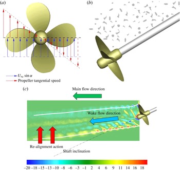
Wake perturbation effects: $P$ -factor (a), onset flow effect (b), main flow effect (c). The contour plot in (c) shows the normalized phase-locked averaged out-of-plane component of the vorticity ( $\langle \unicode[STIX]{x1D714}_{y}\rangle D/U_{tip}$ , where $U_{tip}=n\unicode[STIX]{x03C0}D=6.75~\text{m}~\text{s}^{-1}$ , $n=$ propeller rotational speed and $D=$ propeller diameter). White lines represent the boundary of the propeller stream tube.

Figure 3.

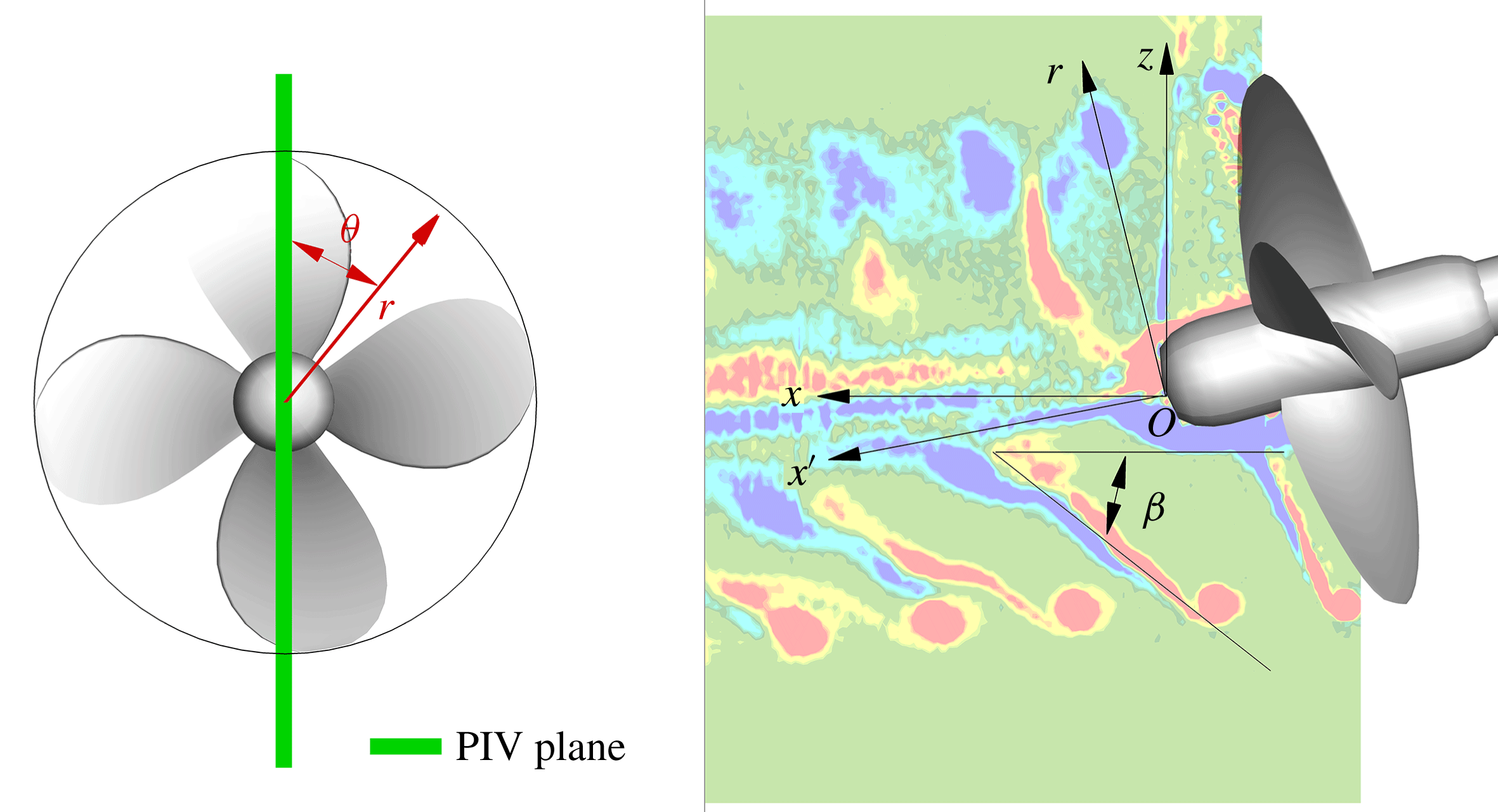
(a) Reference frames. (b) The contour plot shows the normalized phase-locked averaged out-of-plane component of the vorticity ( $\langle \unicode[STIX]{x1D714}_{y}\rangle D/U_{tip}$ ); $\unicode[STIX]{x1D6FD}$ represents the pitch angle of the blade wake.

A simplified model of the real operating conditions of a rotor is represented by the oblique flow configuration, i.e. a rotor operating in a pusher configuration with the hub cap pointing downstream, which implies the following major effects (figure 2):

(i) $P$ -factor: the misalignment of the flow with the rotor axis implies each blade experiences unsteady loading conditions during a revolution (for example, when the rotor is tilted downwards, the downgoing blade meets the relative flow at a higher angle of attack than the upgoing blade, and thus develops more thrust). The relationship between the inclination angle of the rotor $\unicode[STIX]{x1D6FC}$ and the hydrodynamic incidence angle $\unicode[STIX]{x1D719}$ of the blade sections in unperturbed inflow conditions is described mathematically as follows:
(1.1) $$\begin{eqnarray}\unicode[STIX]{x1D711}(r,\unicode[STIX]{x1D703},\unicode[STIX]{x1D6FC})=\unicode[STIX]{x1D6F9}(r)-\tan ^{-1}\left(\frac{U_{\infty }\cos \unicode[STIX]{x1D6FC}}{2\unicode[STIX]{x03C0}nr+U_{\infty }\sin \unicode[STIX]{x1D6FC}\cos \unicode[STIX]{x1D703}}\right)-\unicode[STIX]{x1D6F9}_{i}(r,\unicode[STIX]{x1D703},\unicode[STIX]{x1D6FC}),\end{eqnarray}$$
where $\unicode[STIX]{x1D6F9}(r)$ is the geometric pitch of the blade section, $\unicode[STIX]{x1D703}$ is the angular position of the blade, as reported in figure 3, and $\unicode[STIX]{x1D6F9}_{i}(r,\unicode[STIX]{x1D703},\unicode[STIX]{x1D6FC})$ is the downwash angle. The dependence of hydrodynamic incidence on the blade position when $\unicode[STIX]{x1D6FC}\neq 0$ is manifested by a variable circulation over the blade which causes shedding of secondary vortical structures according to the mechanism described in Di Mascio et al. (Reference Di Mascio, Muscari and Dubbioso2015).
(ii) Onset flow non-uniformity and turbulence effect: propeller onset flow non-uniformity, due to vorticity and turbulent eddies shed from the inclined shaft, generates a narrow and highly unsteady perturbation which locally interferes with the blades, modifying the wake morphology and the loading distribution (Huyer & Snarski Reference Huyer and Snarski2003). Moreover, the interaction between the unsteady turbulent inflow and the rotor produces unsteady forces on the blades along with the generation of unsteady distortion noise, as documented in Robison & Peake (Reference Robison and Peake2014). The variable inflow conditions to which blades are exposed imply a local variation of the hydrodynamic incidence, and thus secondary vorticity shedding due to the consequential local variations of the blade circulation (Felli & Di Felice Reference Felli and Di Felice2005).
(iii) Main flow effect: in oblique flow conditions, the rotor wake is affected by interference with the main flow which tends to suppress the initial misalignment of the wake stream tube (i.e. the vortex sheet tube that separates the undisturbed flow from the flow passing through the rotor) with the free stream. This interference is such as to locally increase/reduce the spiral-to-spiral distance of the wakes shed from two contiguous blades in the windward/leeward region, thus influencing the mutual inductance between adjacent tip vortices (Felli et al. Reference Felli, Camussi and Di Felice2011).

These effects make the simplified configuration of a rotor in inclined flow conditions a case study worth an in-depth investigation for understanding the underlying mechanisms of the wake behaviour in off-design conditions, as stated in Di Mascio et al. (Reference Di Mascio, Muscari and Dubbioso2015).

In the present study, the simplified model of a rotor mounted backwards on a shaft and operating in oblique flow was used to investigate experimentally the influence of inflow unsteadiness and turbulence on wake evolution, destabilization and breakdown. In particular, emphasis was placed on studying the connection between inflow perturbation, the trailing wake characteristics and instability of the tip and root vortices. To this end, detailed flow measurements by a multicamera particle image velocimetry (PIV) system were undertaken in a meridian plane of the wake from the blade trailing edge up to 4.5 rotor diameters downstream, for different rotor inclinations (i.e. $\unicode[STIX]{x1D6FC}=0^{\circ }$ , $\unicode[STIX]{x1D6FC}=7.5^{\circ }$ , $\unicode[STIX]{x1D6FC}=15^{\circ }$ , $\unicode[STIX]{x1D6FC}=25^{\circ }$ ). The multicamera arrangement ensured a large domain of interest could be acquired simultaneously at a vector grid resolution adequate to resolve the dynamics of the small-scale eddies of the blade wake. The experiment, which uses the same test case adopted in Felli et al. (Reference Felli, Camussi and Di Felice2011) and recently in Di Mascio et al. (Reference Di Mascio, Muscari and Dubbioso2015), was carried out in a circulating water channel whose large dimensions avoided blockage effects that could jeopardize the reliability of the results.

The paper is organized as follows. Reference frames and dimensionless groups are described in § 2. Section 3 gives an overview of the experiment. The facility is described in § 3.1. Section 3.2 details the rotor geometry and its arrangement in the facility. Section 3.3 presents the PIV measurements, including the experimental set-up, camera arrangement, image-processing procedures and uncertainty assessment. Test matrix and conditions are documented in § 4. The results are discussed in three subsections of § 5, namely the nominal wake flow in § 5.1, the mean and instantaneous flow distributions in § 5.2 and the wake dynamics in § 5.3. Conclusions and future work are finally discussed in § 6.

2 Reference frames and dimensionless groups

Two reference systems were adopted (see figure 3):

(i) an inertial reference frame $O-xyz$ with the origin $O$ at the intersection between the aft end of the propeller boss and the rotation axis, the $x$ -axis downstream-oriented along the channel centreline, the $z$ -axis pointing upward vertically, and the $y$ -axis following the right-hand rule;
(ii) a cylindrical reference frame $O-x^{\prime }r\unicode[STIX]{x1D703}$ with the origin $O$ at the intersection between the aft end of the propeller boss and the rotation axis, the $x^{\prime }$ -axis downstream-oriented along the propeller axis, the $r$ -axis radially outwards, and the $\unicode[STIX]{x1D703}$ -axis along the azimuth.

All the quantities are made non-dimensional using the following reference values: the propeller diameter ( $D=0.227~\text{m}$ ), the velocity at the blade tip ( $U_{tip}=n\unicode[STIX]{x03C0}D=6.75~\text{m}~\text{s}^{-1}$ ) and the fluid density ( $\unicode[STIX]{x1D70C}=1000~\text{kg}~\text{m}^{-3}$ ).

The flow field is basically governed by two non-dimensional groups:

(i) the effective advance ratio $J=U_{\infty }/(nD\cos \unicode[STIX]{x1D6FC})=0.67$ , where $U_{\infty }$ is the free-stream velocity, $\unicode[STIX]{x1D6FC}$ the shaft inclination angle, $n$ the revolution speed and $D$ the propeller diameter;
(ii) the Reynolds number $Re=c_{0.7}V_{0.7}/\unicode[STIX]{x1D708}=500\times 10^{3}$ , where $\unicode[STIX]{x1D708}$ is the kinematic viscosity, $c_{0.7}$ is the blade chord and $V_{0.7}=\sqrt{(U_{\infty }/\cos \unicode[STIX]{x1D6FC})^{2}+(\unicode[STIX]{x03C0}n(0.35D))^{2}}$ is the velocity at $0.35D$ .

3 Experimental set-up

3.1 Facility

The experiment was performed in the large circulating water tunnel of CNR INSEAN. The test section is 12 m long, 3.6 m wide and 2.25 m deep. The water flow is driven by two axial pumps requiring a total power of approximately 980 KW at the maximum water speed of $5.3~\text{m}~\text{s}^{-1}$ . The highest free-stream turbulence intensity in the test section is less than 4 %. In the test section, the mean velocity uniformity is within 2 % for the axial component and 4 % for the cross-components.

3.2 Case study

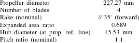
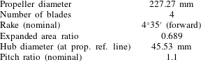
The case study selected for this study is a naval propeller, namely the INSEAN E779A model (Salvatore et al. Reference Salvatore, Pereira, Felli, Calcagni and Di Felice2006). This is a reference four-bladed, fixed-pitch, right-handed propeller model characterized by a nominal constant pitch distribution and a low skew, already used in prior experimental (Felli et al. Reference Felli, Camussi and Di Felice2011) and numerical works (Dubbioso, Muscari & Di Mascio Reference Dubbioso, Muscari and Di Mascio2014) aimed at investigating the mechanisms of rotor wake destabilization. In fact, this propeller, highly loaded at the tip, generates strong tip vortices and, hence, is particularly suitable for the study of the wake instability and breakdown phenomena, where the dynamics of the tip vortices plays an important role. A view of the propeller is shown in figure 4. The main geometrical parameters are documented in table 1.

The propeller was mounted backwards in the typical push-type arrangement, as documented in figure 5. Although this configuration yields inhomogeneous inflow conditions due to wake shedding from the nacelle and the shaft, it was preferred over the pull-type arrangement (i.e. propeller mounted forward, in front of the shaft) in which the shaft interferes with the propeller wake, and thus alters its characteristics, even significantly.

Figure 4.

CNR INSEAN E779A propeller.

Figure 5.

Propeller mounting: $h$ and $\unicode[STIX]{x1D6FC}$ represent the submersion and the inclination of the propeller, respectively.

Table 1.

Geometrical characteristics of the CNR INSEAN E779A propeller.

The problem of transmission layout interference was partially overcome by adopting a shaft long enough to ensure the nacelle perturbation, as estimated by a RANS simulation, faded away completely at the propeller location. Thus, the propeller–shaft configuration adopted allowed reduction of the inflow perturbation to only the shaft wake, whose contribution can be easily estimated by considering the model of a circular cylinder at incidence (Surry & Surry Reference Surry and Surry1967).

The propeller-dynamometer system was mounted at the middle of the measurement section. Propeller submersion was kept at a fixed depth of $h=1.5~\text{m}$ , regardless of the inclination angle. This allowed us to avoid propeller wake evolution being influenced by free surface effects.

3.3 PIV measurements

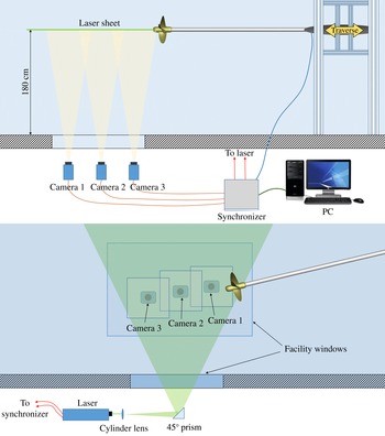
A sketch of the experimental set-up adopted in the PIV measurements is reported in figure 6.

Figure 6.

Top and side views of the PIV experimental set-up.

The illumination was provided by a double-cavity Nd–Yag laser (Quantel Twins, 220 mJ per pulse, 15 Hz repetition rate, wavelength 532 nm). The laser beam was expanded through a combination of a cylindrical diverging lens ( $-15~\text{mm}$ focal length) and a spherical lens (5000 mm focal length) to generate an illumination domain extending approximately $400~\text{mm}\times 10~\text{mm}$ in the streamwise and transversal directions, respectively. The laser was arranged so that the light sheet propagated upwards, through a window placed in the bottom side of the test section (bottom of figure 6).

The scattered light was recorded by a multicamera recording system consisting of three Imager sCMOS cameras by LaVision (16 bits, $2560~\text{pixel}\times 2160~\text{pixel}$ , $6.5~\unicode[STIX]{x03BC}\text{m}$ pixel size, $50~\text{frames}~\text{s}^{-1}$ maximum frame rate). Each camera was equipped with a Nikkor AF-S 85 mm f/1.4G lens by Nikon, set at f/8 aperture. Cameras were arranged side by side in the longitudinal direction with the optical axis perpendicular to the laser sheet. The multicamera configuration allowed simultaneous acquisition of a large flow extent without jeopardizing the spatial resolution of the measurement. 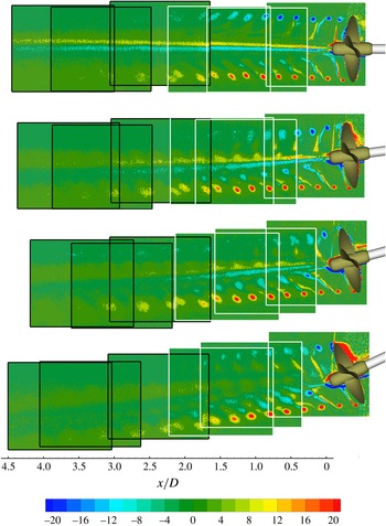More specifically, the spatial domain of $650\times 290~\text{mm}^{2}$ was recorded by overlapping the fields of view of the three cameras in the longitudinal direction by approximately 60 %. The field of view of the camera system allowed coverage of approximately half of the region of interest and thus created the need to split it into two regions, as shown in figure 7. Namely:

(i) a region upstream, indicated by the white rectangles in figure 7, which covers the near and transition regions of the propeller wake up to approximately $x=2.5D$ ;
(ii) a region downstream, indicated by the black rectangles in figure 7, which covers part of the transition region and the far field up to approximately $x=4.5D$ .

Figure 7.

Field of view of the multicamera system used for the PIV measurements (white: camera field of view in the upstream region, black: camera field of view in the downstream region). Contour plots show the normalized phase-locked averaged out-of-plane component of the vorticity ( $\langle \unicode[STIX]{x1D714}_{y}\rangle D/U_{tip}$ ).

For each value of the propeller inclination, the relative camera positions were adjusted to get an optimal reconstruction of the flow in accordance with the local inclination of the propeller stream tube, as documented in figure 7.

The facility water was seeded with hollow glass particles of $10~\unicode[STIX]{x03BC}\text{m}$ diameter and a specific weight of $1.05~\text{g}~\text{cm}^{-3}$ .

The PIV acquisition was conditioned upon the passage of the propeller reference blade for a selected angular position. This was carried out by synchronizing the PIV cameras and the laser pulses to a once-per-revolution TTL signal, supplied by a $3600~\text{pulse}~\text{s}^{-1}$ rotary incremental encoder mounted on the propeller dynamometer. The synchronization was achieved by a programmable timing unit (LaVision PTU).

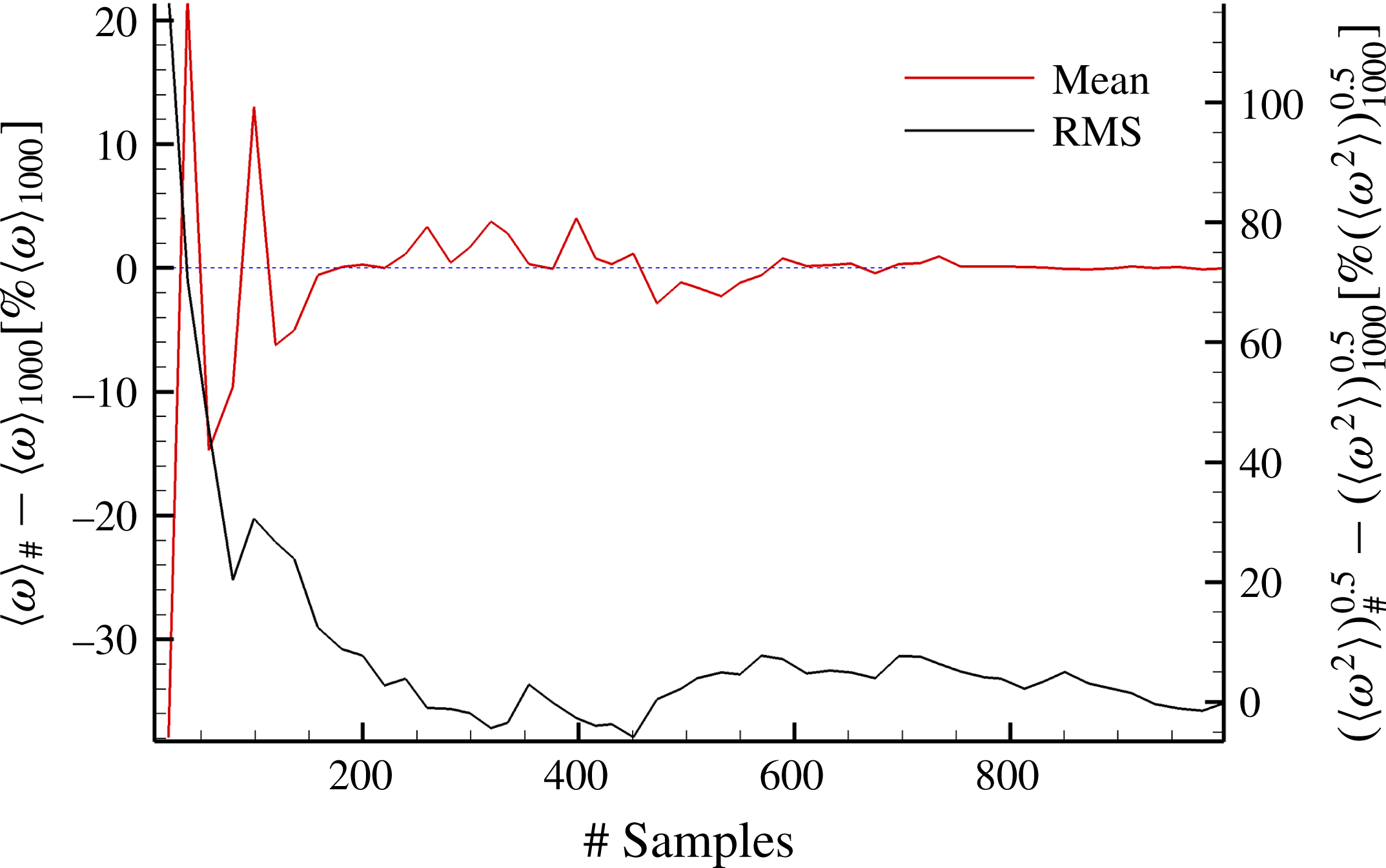
The phase-locked statistical analysis was undertaken over a population of 1000 image pairs, recorded for each propeller position in the range from $0^{\circ }$ to $350^{\circ }$ in steps of $10^{\circ }$ . This choice gave a statistical uncertainty estimated within 0.5 % and 5 % for the first- and second-order estimators (see figure 8). The whole experimental campaign consisted of a total number of 144 000 image pairs, corresponding to approximately 4 TB.

Figure 8.

PIV measurement convergence analysis. Red line represents the percentage deviation between the phase-locked averaged out-of-plane component of the vorticity calculated over # samples (with # ranging from 0 to 1000) ( $\langle \unicode[STIX]{x1D714}\rangle _{\#}$ ) and over 1000 samples ( $\langle \unicode[STIX]{x1D714}\rangle _{1000}$ ). Black line represents the percentage deviation between the phase-locked RMS of the out-of-plane vorticity calculated over # samples ( $\langle \sqrt{\unicode[STIX]{x1D714}^{\prime 2}}\rangle _{\#}$ ) and over 1000 samples ( $\langle \sqrt{\unicode[STIX]{x1D714}^{\prime 2}}\rangle _{1000}$ ).

Data acquisition and processing were performed by a dual ESA-CORE Intel Xeon processor at 2.67 GHz with 48 GB RAM memory.

Recorded images were pre-processed by a local background subtraction routine over a kernel of $4~\text{pixel}\times 4~\text{pixel}$ , followed by a sharpening filter to enhance the shape of particle images. This procedure enhanced the signal-to-noise ratio of the cross-correlation, thus improving the visibility of the seed particles.

The particle field motion was computed using an advanced iterative, multipass direct cross-correlation procedure implemented for GPU processing. Image deformation (Scarano Reference Scarano2002) was applied to each correlation window. Interrogation windows were iteratively reduced to the final size of $24~\text{pixel}\times 24~\text{pixel}$ and then overlapped by 75 %. The resulting vector spacing was 6 pixels, which corresponds to a grid spacing of 0.84 mm.

Vector fields were post-processed at each iteration by applying the universal outlier detection and recursive replacement procedure described in Westerweel & Scarano (Reference Westerweel and Scarano2005).

A rigorous uncertainty analysis for the PIV measurements is out of the scope of the paper. Nonetheless, the topic has been investigated in detail, and a number of works presenting detailed evaluations of PIV measurement errors can be found in the literature (for example, Adrian & Westerweel Reference Adrian and Westerweel2011). The estimated error for the instantaneous velocity field is approximately 3 % of the free-stream velocity.

4 Test conditions

Oblique flow conditions were achieved by varying the shaft inclination in the vertical plane, namely setting the propeller pitch at $\unicode[STIX]{x1D6FC}=0^{\circ }$ , $\unicode[STIX]{x1D6FC}=7.5^{\circ }$ , $\unicode[STIX]{x1D6FC}=15^{\circ }$ and $\unicode[STIX]{x1D6FC}=22.5^{\circ }$ . The corresponding distribution of the hydrodynamic incidence over the blade span is described in (1.1).

During the tests, the effective advance coefficient in the direction of the propeller axis was kept constant, i.e. $J=U_{\infty }/(nD\cos \unicode[STIX]{x1D6FC})$ regardless of the shaft inclination. This allowed us to investigate the effect of propeller inclination at thrust/tip vortex identity, tip vortex dynamics playing a major role in the mechanisms of propeller wake instability (Okulov & Sørensen Reference Okulov and Sørensen2007; Felli et al. Reference Felli, Guj and Camussi2008, Reference Felli, Camussi and Di Felice2011). In practice, the effective advance coefficient was kept constant by scaling the free-stream velocity by $\cos \unicode[STIX]{x1D6FC}$ (i.e. $U_{\infty }(\unicode[STIX]{x1D6FC})=1.45/\cos \unicode[STIX]{x1D6FC}~\text{m}~\text{s}^{-1}$ ) and keeping the propeller rotational speed fixed to $n=9.47~\text{rps}$ .

5 Results

5.1 Nominal wake flow

The present section describes the flow behaviour in the absence of the propeller as measured in a meridian plane of the wake (i.e. nominal wake). The primary focus is to highlight the effect of the shaft inclination on the propeller inflow. To this end, nominal wake tests were undertaken at the same kinematic conditions as used in the presence of the propeller.

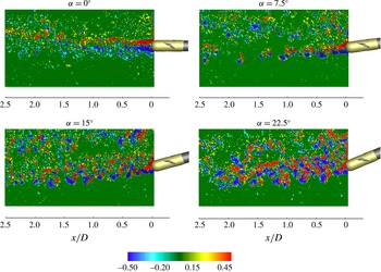
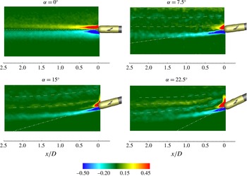
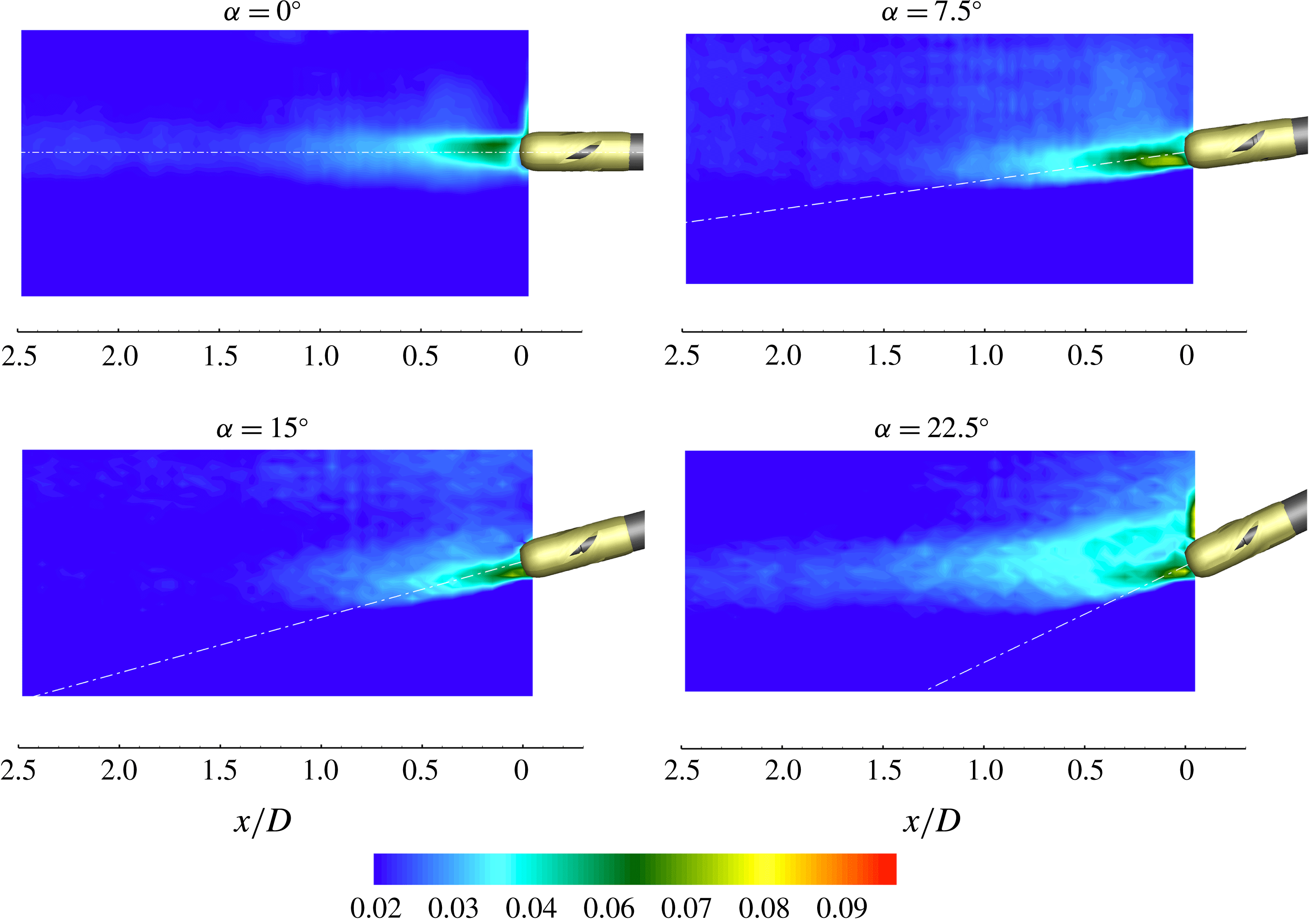
Figures 9 and 10 report the instantaneous and averaged distributions of the out-of-plane vorticity, respectively, for shaft inclinations of $\unicode[STIX]{x1D6FC}=0^{\circ }$ , $\unicode[STIX]{x1D6FC}=7.5^{\circ }$ , $\unicode[STIX]{x1D6FC}=15^{\circ }$ and $\unicode[STIX]{x1D6FC}=22.5^{\circ }$ . The RMS of the out-of-plane vorticity is shown in figure 11.

Figure 9.

Propeller onset flow. Contours of the normalized out-of-plane vorticity $\unicode[STIX]{x1D714}_{y}D/U_{tip}$ at a given instant for $\unicode[STIX]{x1D6FC}=0^{\circ }$ , $\unicode[STIX]{x1D6FC}=7.5^{\circ }$ , $\unicode[STIX]{x1D6FC}=15^{\circ }$ , $\unicode[STIX]{x1D6FC}=22.5^{\circ }$ .

Figure 10.

Propeller onset flow. Contours of the normalized mean out-of-plane vorticity $\bar{\unicode[STIX]{x1D714}}_{y}D/U_{tip}$ for $\unicode[STIX]{x1D6FC}=0^{\circ }$ , $\unicode[STIX]{x1D6FC}=7.5^{\circ }$ , $\unicode[STIX]{x1D6FC}=15^{\circ }$ , $\unicode[STIX]{x1D6FC}=22.5^{\circ }$ .

Inflow perturbation affects the leeward portion of the wake and can be basically modelled as a von Kármán street generated by the cross-flow velocity $U_{\infty }\sin \unicode[STIX]{x1D6FC}$ (i.e. the $Re_{d}$ based on shaft diameter ranges from $Re_{d}(7.5^{\circ })=8\times 10^{3}$ to $Re_{d}(22.5^{\circ })=23\times 10^{3}$ ) through a mechanism similar to that described by Thakur, Liu & Marshall (Reference Thakur, Liu and Marshall2004) for a yawed cylinder, and a system of vortices shed at the trailing-end of the shaft. In contrast, an undisturbed flow condition characterizes the windward part of the measurement plane.

The imprint of the von Kármán vortex street is clearly visible in the averaged field of the out-of-plane vorticity for $\unicode[STIX]{x1D6FC}>0^{\circ }$ , where alternate streaks of positive and negative vorticity are visible in the transversal direction along the leeward side (see dashed lines in figure 10). This pattern is clearly associated with the wavy nature of the von Kármán wake vortices as documented in Marshall (Reference Marshall2003).

The intensity and topology of the nominal wake flow are noticeably dependent on the shaft inclination. At $\unicode[STIX]{x1D6FC}=0^{\circ }$ , the inflow perturbation is localized downstream of the shaft-end and shows a symmetrical topology, on average, in the leeward and windward regions of the wake (figures 10 and 11).

Figure 11.

Propeller onset flow. Contours of the normalized RMS of the out-of-plane vorticity $\sqrt{\overline{{\unicode[STIX]{x1D714}^{\prime }}_{y}^{2}}}D/U_{tip}$ for $\unicode[STIX]{x1D6FC}=0^{\circ }$ , $\unicode[STIX]{x1D6FC}=7.5^{\circ }$ , $\unicode[STIX]{x1D6FC}=15^{\circ }$ , $\unicode[STIX]{x1D6FC}=22.5^{\circ }$ .

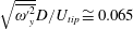
In contrast, the trace of the vortex sheet shed from the trailing-end of the shaft manifests a progressively asymmetric distribution when the inclination angle is increased. In particular, the vorticity field is dominated by a sheet of negative vorticity whose trace is suddenly deflected by the effect of the main flow. This behaviour is consistent with the typical wake flow topology of a slender body in inclined flow operation (Chih-Chung Reference Chih-Chung1990). This vortex sheet tends to become rapidly aligned with the main flow within 1–1.5 propeller diameters, depending on the inclination angle (see figures 9 and 10). The strength of the inflow vortices is approximately one order of magnitude weaker than that of the propeller wake structures (i.e. tip and hub vortices, blade trailing wake). The levels of the out-of-plane vorticity fluctuations are higher in the wake of the propeller boss (i.e. $\sqrt{\overline{{\unicode[STIX]{x1D714}^{\prime }}_{y}^{2}}}D/U_{tip}\cong 0.065$ ) and then reduce significantly in the downstream direction after $0.4{-}0.5D$ (i.e. 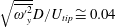$\sqrt{\overline{{\unicode[STIX]{x1D714}^{\prime }}_{y}^{2}}}D/U_{tip}\cong 0.04$ around $x/D=0.5$ , 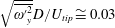$\sqrt{\overline{{\unicode[STIX]{x1D714}^{\prime }}_{y}^{2}}}D/U_{tip}\cong 0.03$ around $x/D=1$ and 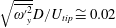$\sqrt{\overline{{\unicode[STIX]{x1D714}^{\prime }}_{y}^{2}}}D/U_{tip}\cong 0.02$ around $x/D=1.5$ ). The propeller inclination does not significantly influence the distribution or behaviour of the vorticity fluctuations for $\unicode[STIX]{x1D6FC}<15^{\circ }$ . When the propeller inclination is increased further ( $\unicode[STIX]{x1D6FC}=22.5^{\circ }$ ), the vorticity fluctuations associated with the von Kármán street generated by the inclined shaft lead to an appreciable thickening and lengthening of the turbulent wake, as shown in figure 11 (i.e. 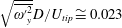$\sqrt{\overline{{\unicode[STIX]{x1D714}^{\prime }}_{y}^{2}}}D/U_{tip}\cong 0.023$ at $x=2.5D$ ).

5.2 Mean and instantaneous flow distribution

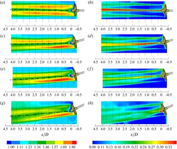
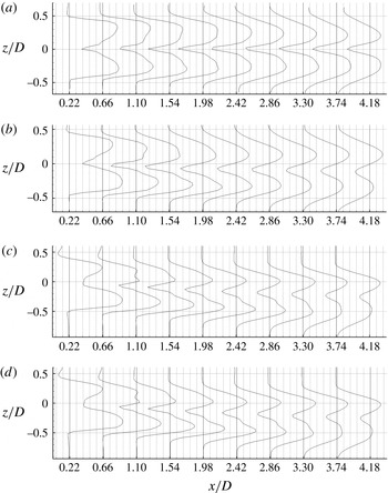
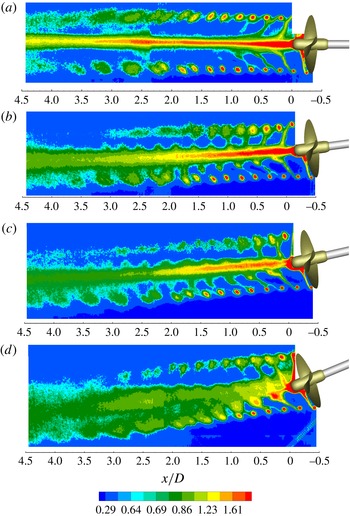
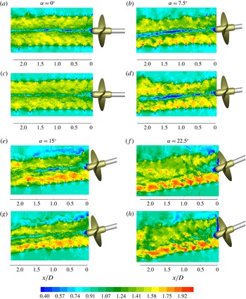
Figure 12 shows the contours of the time-averaged streamwise velocity and the turbulence intensity for $\unicode[STIX]{x1D6FC}=0^{\circ }$ , $7.5^{\circ }$ , $15^{\circ }$ and $22.5^{\circ }$ . The instantaneous streamwise velocity distributions are reported in figure 13. The profiles of the streamwise velocity and the turbulent intensity, extracted at the locations indicated by dotted lines in figure 12, are shown in figures 14 and 15. Velocities are normalized with the free-stream velocity $U_{\infty }(\unicode[STIX]{x1D6FC})=1.45/\text{cos}\,\unicode[STIX]{x1D6FC}$ . The turbulence intensity is defined as $I_{x}=\unicode[STIX]{x1D70E}_{x}/U_{\infty }(\unicode[STIX]{x1D6FC})$ , where $\unicode[STIX]{x1D70E}_{x}$ is the standard deviation of the streamwise velocity.

Figure 12.

Evolution of the normalized mean streamwise velocity ( $\bar{u}/U_{\infty }$ ) (a,c,e,g) and of the turbulent intensity ( $\unicode[STIX]{x1D70E}_{x}/U_{\infty }$ ) (b,d,f,h) for $\unicode[STIX]{x1D6FC}=0^{\circ }$ (a,b), $\unicode[STIX]{x1D6FC}=7.5^{\circ }$ (c,d), $\unicode[STIX]{x1D6FC}=15^{\circ }$ (e,f) and $\unicode[STIX]{x1D6FC}=22.5^{\circ }$ (g,h). Dashed lines indicate the locations where velocity profiles of figures 14 and 15 are extracted. The black dashed-dot lines represent the wake-centre trajectory in the measurement plane obtained from the velocity profiles of figure 14 by measuring the distance between the positions where the flow velocity exceeds the free-stream velocity by 5 %.

Figure 13.

Snapshots of the normalized streamwise velocity ( $u/U_{\infty }$ ) at a given propeller phase (i.e. the two snapshots are relative to two instants at the same propeller position) for $\unicode[STIX]{x1D6FC}=0^{\circ }$ (a,c), $\unicode[STIX]{x1D6FC}=7.5^{\circ }$ (b,d), $\unicode[STIX]{x1D6FC}=15^{\circ }$ (e,g) and $\unicode[STIX]{x1D6FC}=22.5^{\circ }$ (f,h).

Figure 14.

Profiles of the normalized streamwise velocity ( $\bar{u}/U_{\infty }$ ) downstream of the propeller for $\unicode[STIX]{x1D6FC}=0^{\circ }$ , $7.5^{\circ }$ , $15^{\circ }$ and $22.5^{\circ }$ (from a to d respectively) for different downstream positions. For each position, $\bar{u}/U_{\infty }=1$ on the vertical thick black line. The width of the grid squares corresponds to $0.088U_{\infty }$ .

Figure 15.

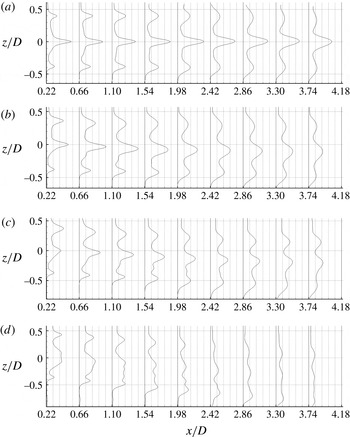
Profiles of the turbulent intensity ( $I_{x}$ ) downstream of the propeller for $\unicode[STIX]{x1D6FC}=0^{\circ }$ , $7.5^{\circ }$ , $15^{\circ }$ and $22.5^{\circ }$ (from a to d respectively) for different downstream positions. For each position, $I_{x}=I_{\infty }$ ( $I_{\infty }=$ facility turbulence, see § 3.1) on the vertical thick black line. The width of the grid squares corresponds to $0.088U_{\infty }$ .

In uniform inflow conditions ( $\unicode[STIX]{x1D6FC}=0^{\circ }$ ), the velocity field is axisymmetric and is dominated by the effect of the flow acceleration induced by the propeller, which presents a maximum corresponding to the sections where blades deliver the maximum thrust (i.e. $r\cong 0.35D$ ) and by a defect in the inner sections of the wake ( $-0.2D<r<0.2D$ ), which is due to the presence of the hub vortex. This gives the characteristic ‘camel-hump’ profile of the mean streamwise velocity distribution behind a propeller. The velocity peaks reduce and become broader as the wake moves downstream, due the effect of turbulent diffusion (figures 12 and 14).

When the propeller operates in inclined flow conditions, the wake undergoes an increasing deflection with increasing inclination angle (i.e. at $x/D=4.18$ the wake centre is at $z/D=-0.08$ for $\unicode[STIX]{x1D6FC}=7.5^{\circ }$ , $z/D=-0.28$ for $\unicode[STIX]{x1D6FC}=15^{\circ }$ and $z/D=-0.35$ for $\unicode[STIX]{x1D6FC}=22.5^{\circ }$ ) and shows a progressively asymmetric distribution of the mean and turbulent fields (figures 12, 14 and 15).

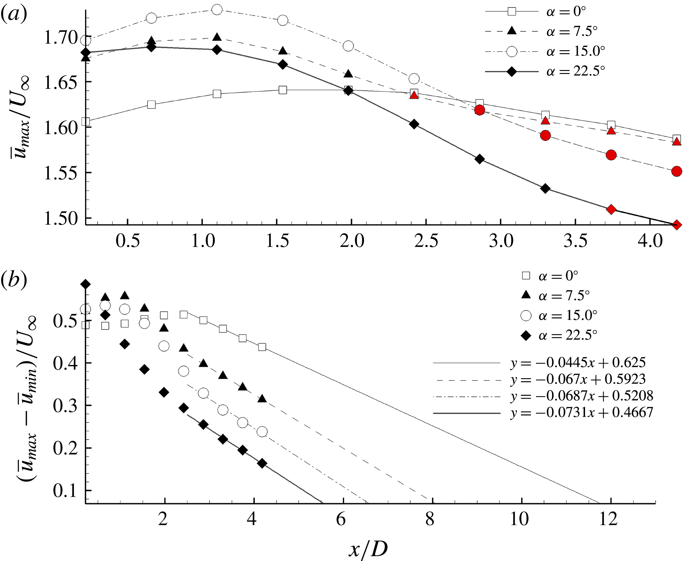
The asymmetry of the streamwise velocity field is mainly ascribable to the effect of the wake swirl which is such as to rotate the flow region clockwise where propeller blades deliver the maximum ( $y>0$ ) and minimum thrust ( $y<0$ ) and where the flow presents the maximum and minimum values of the velocity, respectively. This leads to the out-of-phase alternation of flow regions with higher and lower velocities which is observed on the windward and leeward sides of the wake, as shown on the figures 12 and 14. Specifically, the local maximum of the streamwise velocity is initially located on the windward side of the wake for $x<x^{\ast }$ (with $x^{\ast }(7.5^{\circ })\cong 2D$ , $x^{\ast }(15^{\circ })\cong 2.5D$ and $x^{\ast }(22.5^{\circ })\cong 3D$ ) and then moves to the leeward side for $x>x^{\ast }$ (see red symbols on figure 16 a) while reducing its intensity gradually downstream. The effect of turbulent diffusion causes a gradual reduction of the velocity gap between the regions with maximum velocity and the wake centre, which is estimated to be zero at approximately $x=14.04D$ for $\unicode[STIX]{x1D6FC}=0^{\circ }$ , $x=8.84D$ for $\unicode[STIX]{x1D6FC}=7.5^{\circ }$ , $x=7.58D$ for $\unicode[STIX]{x1D6FC}=15^{\circ }$ and $x=6.38D$ for $\unicode[STIX]{x1D6FC}=22.5^{\circ }$ , respectively, according to a linear regression fit (see figure 16 b). Further downstream, wake profiles are considered to gradually evolve into a bell-shaped distribution and to approach a self-similar behaviour, analogously to any jet in co-flow (Rajaratnam Reference Rajaratnam1976).

The distribution of the turbulence intensity $I_{x}$ exhibits a tri-peak pattern with a dominant peak around the central region of the wake, which is associated with the high turbulence levels produced by the hub vortex, and two weaker peaks corresponding to tip vortex traces on the leeward and windward sides of the wake (figure 15). The relative magnitudes of the turbulence peaks associated with the hub vortex and with the tip vortices show a clear dependence on the inclination angle, tending to reduce as the propeller inclination increases (figure 15). Furthermore, the profiles of the turbulence peaks undergo gradual smoothing with respect to the distance from the propeller disk with a rate that increases when the propeller inclination is increased, as shown on figure 12(b,d,f,h).

The locations where the wake is estimated to assume a bell-shaped profile indicate that the wake recovery of propellers is much slower compared to wind turbines, where it is typically observed a few diameters downstream of the rotor (see, for example, Bastankhah & Porté-Agel Reference Bastankhah and Porté-Agel2016).

Furthermore, unlike the wake of a wind turbine, in which the velocity deficit at the centre recovers within a few rotor diameters and in which the interior of the wake consists of a low and broad amount of turbulence, the distribution of both the velocity and the turbulent intensity in the propeller wake is dominated by the contribution of the hub vortex, which persists for several propeller diameters in the downstream direction, as inferable from the contour plots of figure 12. This result highlights a substantial difference in the wake characteristics of rotor systems adding and subtracting energy to and from the flow, which involves also the opposite rotation of the wake with respect to the rotor and the respectively smaller and larger skew angle of the wake with respect to the rotor inclination, as shown in § 5.3.

Figure 16.

Evolution of the maximum of the mean streamwise velocity $\bar{u}_{max}/U_{\infty }$ (a) and of the velocity gap between maximum and minimum values of the mean streamwise velocity $(\bar{u}_{max}-\bar{u}_{min})/U_{\infty }$ (b) for $\unicode[STIX]{x1D6FC}=0^{\circ }$ , $\unicode[STIX]{x1D6FC}=7.5^{\circ }$ , $\unicode[STIX]{x1D6FC}=15^{\circ }$ , $\unicode[STIX]{x1D6FC}=22.5^{\circ }$ . Symbols on the top of the figure are coloured in red when the velocity maximum is located on the leeward side. Linear fits are used to estimate the position where the velocity gap is zero.

5.3 Wake dynamics

The dynamic evolution of the propeller vortices is the subject of the present section, whose primary focus is on highlighting the mechanisms underlying propeller wake evolution and instability in oblique inflow conditions. To this end, the propeller wake is analysed on the basis of the mean (phase-locked) and instantaneous flow-field characteristics under different oblique flow conditions, for a wake extent covering the near field and far field up to approximately 4.5 propeller diameters downstream.

Figure 17.

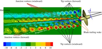
Sketch of the vortex systems in the wake of a propeller operating in inclined flow condition. Contour plot shows the normalized phase-locked averaged out-of-plane component of the vorticity $\langle \unicode[STIX]{x1D714}_{y}\rangle D/U_{tip}$ .

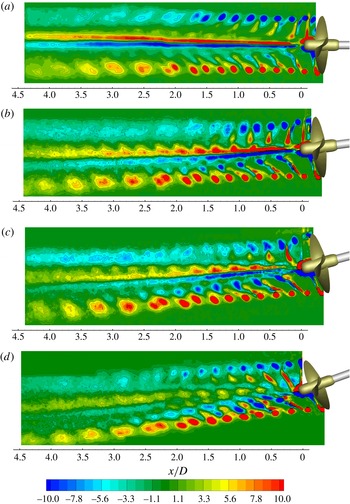
Figure 17 shows a representative overview of the major vortical systems in a meridian section of a propeller wake in oblique flow conditions (i.e. $\unicode[STIX]{x1D6FC}=15^{\circ }$ ). In particular, these are as follows.

(i) A system of strong coherent vortices shed from the blade tips whose traces exhibit opposite signs of the out-of-plane vorticity on the leeward and windward sides of the wake (i.e. tip vortices).
(ii) An intense vortical tube streaming aft of the hub which is formed by the coalescence of root vortices shed from the blades and which involves the shear layers detached from the hub (i.e. hub vortex).
(iii) A system of coherent horseshoe vortices formed at the blade leading edge junction with the hub which describe a helical trajectory as they are convected downstream. The generation mechanism of these vortical structures is well documented in Gand et al. (Reference Gand, Deck, Brunet and Sagaut2010) and is inferable from figure 2 of Budich, Schmidt & Adams (Reference Budich, Schmidt and Adams2015) and from figure 9 of Aeschlimann et al. (Reference Aeschlimann, Beaulieu, Houde, Dan Ciocan and Deschenes2013). The signature of this vortical system presents opposite signs of the out-of-plane vorticity on the leeward and windward sides of the wake and delineates a diverging spiral when the propeller operates in oblique flow conditions. We refer to these vortices as ‘junction vortices’.
(iv) A system of small-scale eddies due to spanwise variation of the circulation $\unicode[STIX]{x1D6E4}$ over the blade that is shed from the blade trailing edge. This vortical system is represented by two counter-rotating vorticity layers which overlap at the radial distance of maximum bound circulation. We refer to these vortices as ‘blade wake’ or ‘trailing wake’.
(v) A secondary vortical system due to the time-dependent nature of the blade circulation which leaves the blade parallel to the trailing edge. This vortical system can be modelled as a succession of vortex rings of variable intensity (according to Helmholtz’s vortex laws) whose resultant in the direction parallel to the trailing edge is non-zero when the blade experiences a variation in the hydrodynamic load (see Di Mascio et al. Reference Di Mascio, Muscari and Dubbioso2015). We refer to this vortical system as ‘shed vorticity’ (see figure 1).

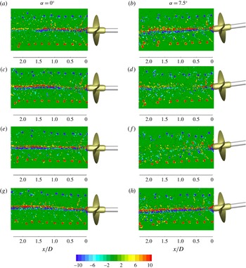
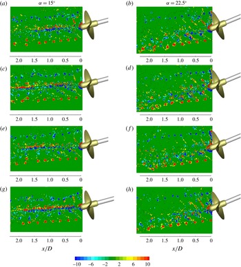
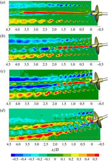
The phase-locked and instantaneous distributions of the vorticity field are shown in figure 18 and in figures 19 and 20 for different values of the inclination angle (i.e. $\unicode[STIX]{x1D6FC}=0^{\circ }$ , $7.5^{\circ }$ , $15^{\circ }$ and $22.5^{\circ }$ ).

Propeller wake dynamics is characterized by an initial regular evolution of the vortical systems which holds until the wake destabilizes. In this region, known as ‘near wake’ (see Jessup Reference Jessup1989), the traces of the tip vortices recur approximately in the same position, instant by instant. The random fluctuations observed in figures 19 and 20 for the instantaneous tip vortex traces before the destabilization are ascribable to a small-scale meandering motion (Del Pino et al. Reference Del Pino, Parras, Felli and Fernandez-Feria2011; Chamorro et al. Reference Chamorro, Hill, Morton, Ellis, Arndt and Sotiropoulos2013). The effect of meandering is also evident in the instantaneous signatures of the hub vortex, which already exhibit spatial fluctuations and deformations in the near field while maintaining a stable behaviour on average. The spatial variation in the vorticity intensity, which is observed along the traces of the hub vortex in figures 19 and 20, is ascribable to the associated out-of-plane meandering, which makes the angle spatially and temporally variable at which the hub vortex is cut by the measurement plane. The same explanation applies to the variable intensity of the streamwise velocity defect associated with the hub vortex in figure 13. The effect of hub vortex meandering appears progressively pronounced when increasing the propeller inclination.

Further downstream, in the transition and far fields, the effect of wake destabilization makes the traces of the tip vortices progressively irregular and with increasingly large spatial fluctuations. The transition from the regular to irregular trend shows a clear dependence on the propeller inclination and occurs after a distance that reduces progressively when increasing the propeller deflection. An estimate based on the vorticity snapshots shows this transition to occur around $x/D=0.7{-}0.8$ for $\unicode[STIX]{x1D6FC}=0^{\circ }$ , $x/D=0.6{-}0.7$ for $\unicode[STIX]{x1D6FC}=7.5^{\circ }$ , $x/D=0.3{-}0.4$ for $\unicode[STIX]{x1D6FC}=15^{\circ }$ and $x/D=0.2{-}0.3$ for $\unicode[STIX]{x1D6FC}=22.5^{\circ }$ .

Figure 18.

Phase-locked evolution of the normalized out-of-plane vorticity ( $\langle \unicode[STIX]{x1D714}_{y}\rangle D/U_{tip}$ ) for $\unicode[STIX]{x1D6FC}=0^{\circ }$ , $\unicode[STIX]{x1D6FC}=7.5^{\circ }$ , $\unicode[STIX]{x1D6FC}=15^{\circ }$ , $\unicode[STIX]{x1D6FC}=22.5^{\circ }$ (from a to d).

Figure 19.

Snapshots of the normalized out-of-plane vorticity ( $\unicode[STIX]{x1D714}_{y}D/U_{tip}$ ) at a given propeller phase (i.e. the four snapshots are relative to four instants at the same propeller position) for $\unicode[STIX]{x1D6FC}=0^{\circ }$ (a,c,e,g) and $\unicode[STIX]{x1D6FC}=7.5^{\circ }$ (b,d,f,h).

Figure 20.

Snapshots of the normalized out-of-plane vorticity ( $\unicode[STIX]{x1D714}_{y}D/U_{tip}$ ) at a given propeller phase (i.e. the four snapshots are relative to four instants at the same propeller position) for $\unicode[STIX]{x1D6FC}=15^{\circ }$ (a,c,e,g) and $\unicode[STIX]{x1D6FC}=22.5^{\circ }$ (b,d,f,h).

The effect of the inclination angle is clearly manifested in the progressively asymmetric evolution of the vortex systems on the leeward and windward sides of the wake when the propeller deflection is increased (figures 18–20). The asymmetry principally concerns the different topology of the blade wake and of the tip and junction vortices, as well as the position of instability inception and the mechanisms by which propeller wake destabilizes, as better detailed below. The more rapid smoothing observed in the phase-locked averaged contours of the tip vortices on the leeward side is ascribable to the effect of the inflow perturbation, however, which causes an increase of the tip vortex fluctuations around their statistically averaged positions in the upper region of the measurement plane (figures 19 and 20).

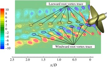
Increasing the propeller inclination does not produce any relevant effect on the hub vortex, however, at least for $\unicode[STIX]{x1D6FC}\leqslant 15^{\circ }$ , as confirmed by the nearly constant intensity of the associated out-of-plane vorticity in figures 18–20. Increasing the inclination further to $\unicode[STIX]{x1D6FC}=22.5^{\circ }$ affects the dynamics of the root vortices significantly, inhibiting their coalescence in a coherent structure, as shown in figure 21.

Figure 21.

Leeward and windward root vortex traces for the propeller inclination $\unicode[STIX]{x1D6FC}=22.5^{\circ }$ . Iso-contours describe the phase-locked normalized out-of-plane vorticity ( $\langle \unicode[STIX]{x1D714}_{y}\rangle D/U_{tip}$ ).

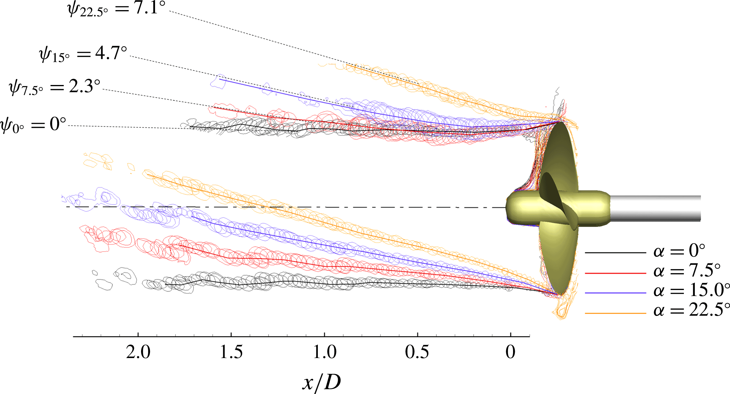
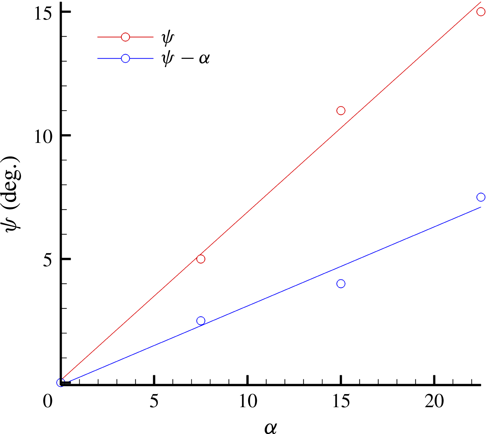
Figure 22 shows the trajectories of the tip vortex traces for $\unicode[STIX]{x1D6FC}=0^{\circ }$ , $\unicode[STIX]{x1D6FC}=7.5^{\circ }$ , $\unicode[STIX]{x1D6FC}=15^{\circ }$ and $\unicode[STIX]{x1D6FC}=22.5^{\circ }$ . Trajectories are educed from the envelope of the tip vortex traces and are represented after a rotation by the opposite of the inclination angle in the vertical plane so that propeller axes relative to different deflections are aligned. Figure 23 reports the slope of the tip vortex trajectories as a function of the propeller inclination.

Figure 22.

Contour lines of the tip vortex traces during a complete propeller revolution for $\unicode[STIX]{x1D6FC}=0^{\circ }$ , $\unicode[STIX]{x1D6FC}=7.5^{\circ }$ , $\unicode[STIX]{x1D6FC}=15^{\circ }$ and $\unicode[STIX]{x1D6FC}=22.5^{\circ }$ . Tip vortex traces are represented after a rotation by the inverse of the inclination angle in the vertical plane. Dashed lines are extrapolated from the envelope profiles of the tip vortices (solid lines) using a linear regression fit. Labels indicate the slopes of the extrapolated lines.

In oblique flow conditions, the propeller wake undergoes a positive deflection relative to the rotation axis. This behaviour is ascribable to the effect of the main flow, which resist the penetration of the propeller wake and tends to align it to the free stream with a mechanism similar to a jet in cross-flow (Mahesh Reference Mahesh2013). The rate of wake deflection, which can be considered indicative of the effectiveness by which the main flow resists wake penetration, increases with the inclination angle according to a linear regression line, as shown in figure 22.

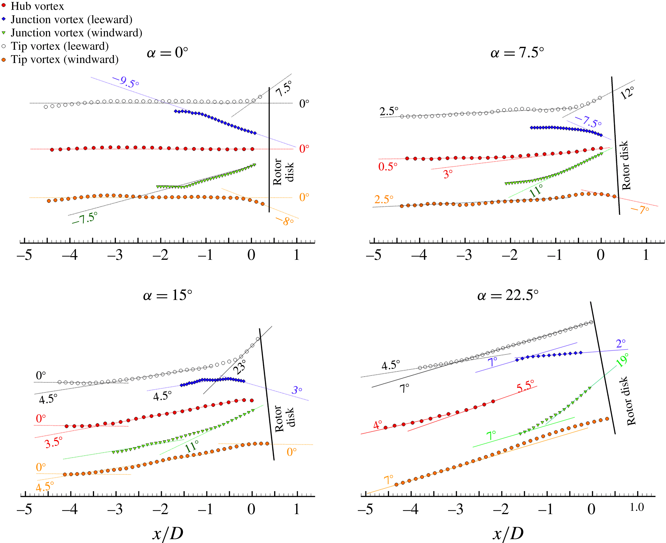
The topological analysis of the vortical systems in the propeller wake highlights the following characteristics (figure 24).

(i) The envelope profiles relative to the phase-locked averaged leeward and windward traces of the tip vortices exhibit approximatively the same slope, with the exception of a limited region just downstream of the trailing edge which is influenced by wake contraction effects.
(ii) Blade junction vortices initially describe a diverging spiral until they approach and interfere with the tip vortices. The interaction of the tip and junction vortices is non-symmetrical in oblique flow conditions and is significantly influenced by the inclination angle. The asymmetry involves the different slopes and strengths of the windward and leeward branches of the junction vortices, which deviate progressively when the inclination angle is increased, as well as the different position at which they interfere with the tip vortices. In particular, at effectively identical $J$ , increasing the inclination angle implies a more intense approach flow encountering the blade–hub junction on the windward side and, correspondingly, the formation of a stronger junction vortex structure (Simpson Reference Simpson2001). The interference positions of the leeward and windward branches of the tip and junction vortices depend on the relative orientation of their trajectories. Specifically, the interference occurs closer to the propeller disk on the leeward side, where the deflection angles of tip and junction vortices have opposite sign. During the interaction, the junction vortices undergo a more or less abrupt deflection until assuming approximately the same slope of the tip vortices.
(iii) The envelope profile of the hub vortex is approximatively aligned with the trace of the wake stream tube, regardless of the inclination angle.

Figure 23.

Propeller wake penetration versus inclination angle. The wake deflection angle for a given propeller inclination is represented by the slope of the linear regression fit of the tip vortex envelope profiles, as reported in figure 22.

Figure 24.

Envelope profiles of the vortex systems in the propeller wake for $\unicode[STIX]{x1D6FC}=0^{\circ }$ , $\unicode[STIX]{x1D6FC}=7.5^{\circ }$ , $\unicode[STIX]{x1D6FC}=15^{\circ }$ and $\unicode[STIX]{x1D6FC}=22.5^{\circ }$ . Scatter plots represent the locus of the vortex centres in the measurement plane. The slopes of the envelope profiles (in magnitude) are indicated by labels.

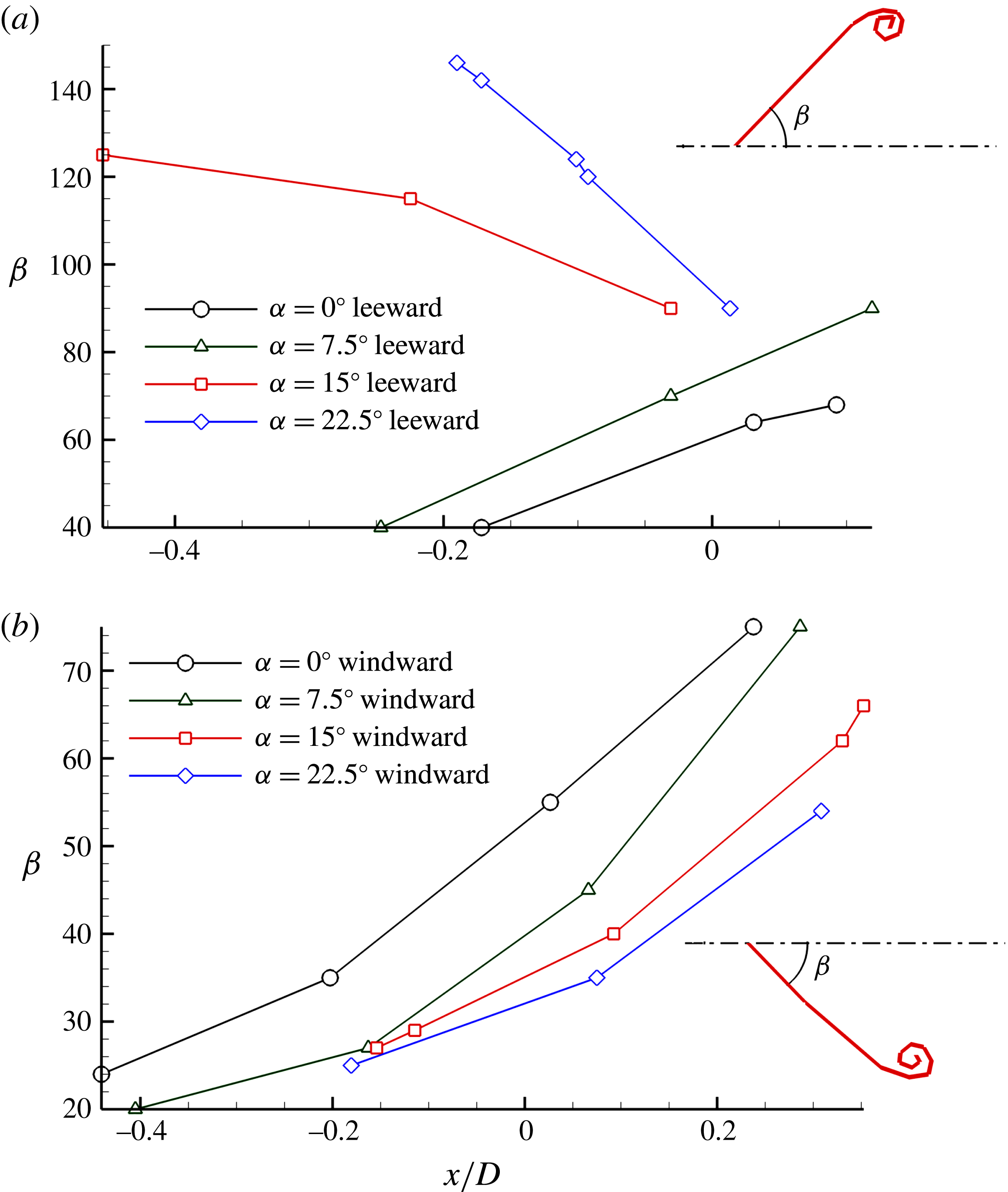
The blade trailing wake manifests a highly distorted morphology from the basic helix that is due to the locally variable convection velocity of the trailing filaments, including the velocity induced by the wake itself. It follows that the bending characteristics of the blade wake will be significantly influenced by the inclination angle of the propeller, as clearly emerges in figure 18.

Figure 25.

Streamwise evolution of the pitch angle of the blade wake ( $\unicode[STIX]{x1D6FD}$ ) for $\unicode[STIX]{x1D6FC}=0^{\circ }$ , $\unicode[STIX]{x1D6FC}=7.5^{\circ }$ , $\unicode[STIX]{x1D6FC}=15^{\circ }$ and $\unicode[STIX]{x1D6FC}=22.5^{\circ }$ . Leeward region (a) and windward region (b). The pitch angle $\unicode[STIX]{x1D6FD}$ is estimated from the slope of the linear regression of the locations of the vorticity peaks along the blade wake trace in the measurement plane.

In the windward region, the blade wake manifests a nearly straight profile whose slope reduces progressively in the streamwise direction, as shown in figure 25(b). Correspondingly, the trailing wake undergoes an increasingly intense stretching which is driven by the significantly different hydrodynamic pitch of the root (larger) and tip (smaller) sections. This implies the tip vortex moves progressively away from the inboard blade wake and from the root vortices in the downstream direction. In the leeward region, the behaviour is substantially similar as long as the inclination angle is smaller than $\unicode[STIX]{x1D6FC}=7.5^{\circ }$ . However, a different trend is observed when the angle of attack is increased further. In this case the trace of the blade wake in the meridian plane assumes a curved profile which is due to the larger hydrodynamic pitch of wake sections where blades deliver the largest circulation/thrust (which are identifiable by the reversed sign of the out-of-plane vorticity) relative to the inboard and outboard sections (see figure 25 a). This leads to a considerable distortion of the wake profile, with a reversed hydrodynamic pitch (i.e. $\unicode[STIX]{x1D6FD}>90^{\circ }$ ) in the inboard sections (see figure 18 for $\unicode[STIX]{x1D6FC}=15^{\circ }$ and $\unicode[STIX]{x1D6FC}=22.5^{\circ }$ ), as shown in figure 26.

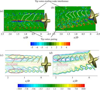
The different hydrodynamic pitch of the tip vortices and the trailing wake implies the tip vortex interferes with the trailing wake shed from the following blade at a certain position. We refer to this interference as to ‘spiral-to-spiral’ or ‘inter-spiral’ interaction.

We conjecture that the aforementioned interaction between the blade wake and the tip vortex of adjacent spirals might be the prelude to the tip vortex destabilization, as already pointed out in Felli et al. (Reference Felli, Di Felice, Guj and Camussi2006), Felli et al. (Reference Felli, Camussi and Di Felice2011) and, recently, in Kumar & Mahesh (Reference Kumar and Mahesh2017). Moreover, this hypothesis is consistent with the conclusion by Okulov & Sørensen (Reference Okulov and Sørensen2007) that the inclusion of the trailing vortex wake produces a stabilizing effect on the unconditionally unstable Joukowsky model of a rotor wake, in which the vorticity is concentrated in $Z$ helical tip vortices ( $Z=$ number of blades) and a hub vortex lying along the rotor axis.

Figure 26.

Hydrodynamic pitch characteristics of the blade trailing wake ( $\unicode[STIX]{x1D6FD}$ ) for $\unicode[STIX]{x1D6FC}=22.5^{\circ }$ . The letter in the superscript and the number in the subscript refer to the portion of the propeller wake (i.e. $W=$ windward, $L=$ leeward) and to the ordinal of the spiral (i.e. increasing with increasing streamwise distance), respectively. Contour plot shows the normalized phase-locked RMS of the axial velocity $\sqrt{\langle u^{\prime 2}\rangle }/U_{tip}$ for $\unicode[STIX]{x1D6FC}=22.5^{\circ }$ .

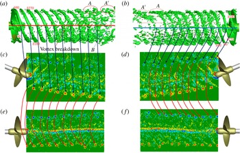
The spiral-to-spiral interaction causes the breakdown of the trailing wake, and thus cancels its stabilizing effect, leading to wake instability. This hypothesis is further supported by the results of Felli et al. (Reference Felli, Guj and Camussi2008), who studied the instability of propellers having the same blade geometry but different numbers of blades, at identical tip vortex strength, and showed that the position of instability inception shifts downstream when the blade number/inter-spiral distance is increased/reduced. Moreover, the mutual-inductance instability (Widnall Reference Widnall1972) is normally observed just downstream of the position where the spiral-to-spiral interference gets underway, as reported in figure 27 and as observed in several animations depicting propeller wake evolution (see, for example, Di Felice et al. Reference Di Felice, Di Florio, Felli and Romano2004).

Figure 27.

Instantaneous contour plot (a,b) and phase-locked averaged (iso-lines on the c,d) representation of the trailing wake deformation and interaction with the tip vortex. Both contours and iso-lines are coloured with the out-of-plane component of the vorticity ( $\langle \unicode[STIX]{x1D714}_{y}\rangle D/U_{tip}$ ) for $\unicode[STIX]{x1D6FC}=0^{\circ }$ (a,c) and $\unicode[STIX]{x1D6FC}=22.5^{\circ }$ (b,d).

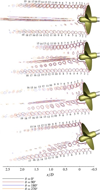
The position of tip vortex instability inception is quantified on the basis of figure 28, which reports the phase-averaged iso-lines of the region with a positive second invariant of $\unicode[STIX]{x1D735}u$ (Hunt, Wray & Moin Reference Hunt, Wray and Moin1988) and the positions of the tip vortex centroids relative to four blade passages, namely $\unicode[STIX]{x1D703}=0^{\circ }$ and $\unicode[STIX]{x1D703}=50^{\circ }$ (first blade passage, coloured in black), $\unicode[STIX]{x1D703}=90^{\circ }$ and $\unicode[STIX]{x1D703}=140^{\circ }$ (second blade passage, coloured in red), $\unicode[STIX]{x1D703}=180^{\circ }$ and $\unicode[STIX]{x1D703}=230^{\circ }$ (third blade passage, coloured in blue), $\unicode[STIX]{x1D703}=270^{\circ }$ and $\unicode[STIX]{x1D703}=50^{\circ }$ (fourth blade passage, coloured in orange).

Both iso-lines and vortex centroid positions relative to the four blade passages appear substantially overlapped as long as the tip vortices remain stable. In fact, tip vortex passage occurs periodically, on average, at the same position in the near field (Felli et al. Reference Felli, Camussi and Di Felice2011).

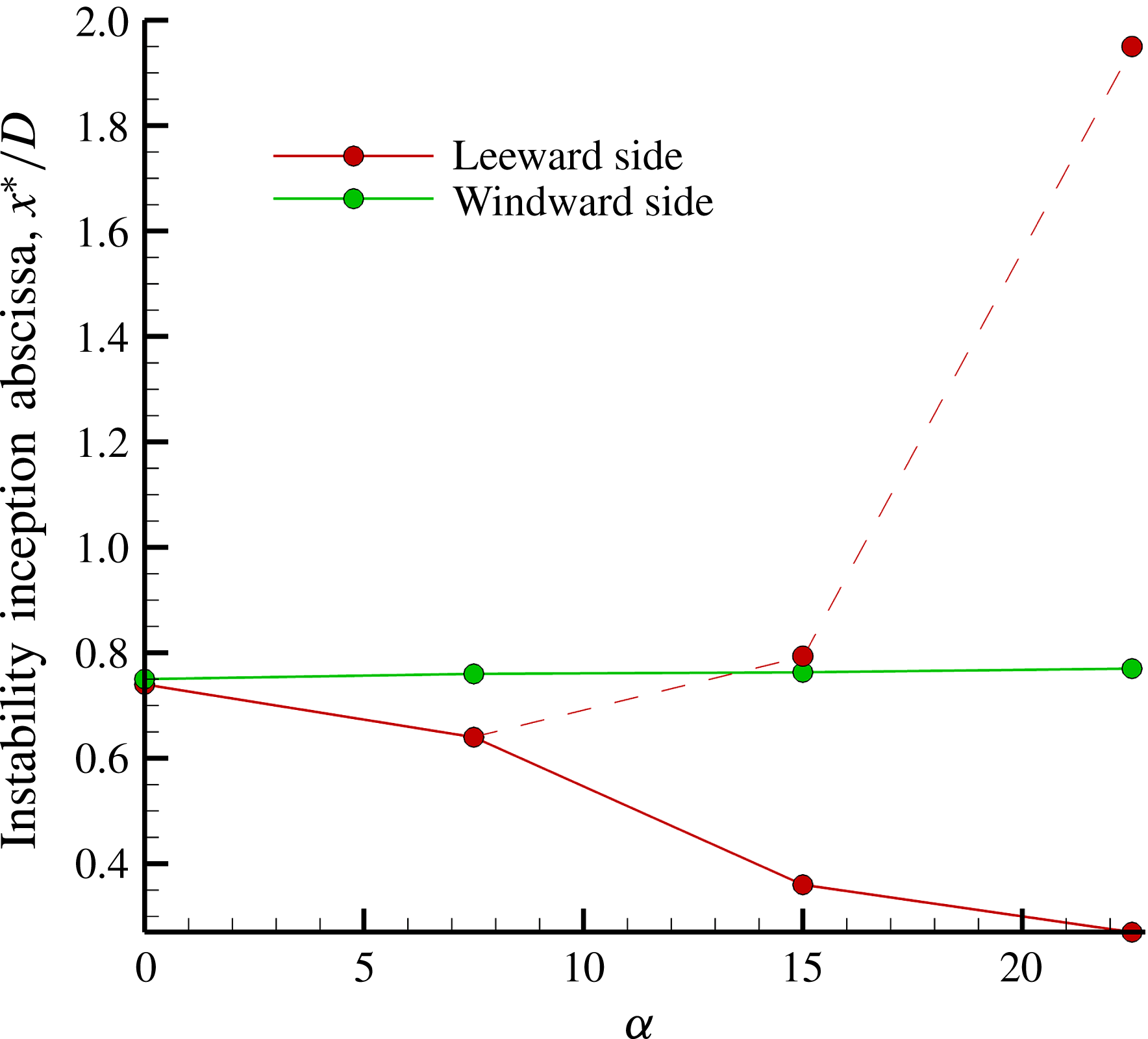
Further downstream, starting from the position of instability inception, iso-lines and vortex centroid positions start to deviate more and more until separating (figure 28). In the current study, the initial position at which tip vortex centroids fall outside a circular domain with diameter $d=0.05D$ is conventionally used to statistically quantify the point of instability inception. The results, educed considering all the phase-averaged tip vortex traces from $0^{\circ }$ to $360^{\circ }$ , are shown in figure 29, which reports the positions of instability inception versus the inclination angle, and confirm the non-symmetrical position of tip vortex instability onset on the leeward and windward sides of the wake and the significant dependence on the propeller inclination.

For $\unicode[STIX]{x1D6FC}=0^{\circ }$ and $\unicode[STIX]{x1D6FC}=7.5^{\circ }$ , instability is initiated by mutual inductance between neighbouring tip vortices which leapfrog over each other according to the mechanism documented in Felli et al. (Reference Felli, Camussi and Di Felice2011). For $\unicode[STIX]{x1D6FC}=0^{\circ }$ , the inception of the mutual inductance occurs symmetrically on the leeward and windward sides of the wake approximately $0.75D$ downstream of the propeller disk, consistent with the results reported in Felli et al. (Reference Felli, Camussi and Di Felice2011) for the same propeller in pure axial inflow conditions. This result confirms that the onset flow perturbation due to the propeller mount does not influence tip vortex instability when the propeller works in straight flow conditions. The shorter distance at which the leeward branches of the tip vortices destabilize compared to the windward ones, when the propeller is inclined by $\unicode[STIX]{x1D6FC}=7.5^{\circ }$ , can be explained by considering that the propeller stream-tube deflection due to the realignment action of the main flow slightly reduces (increases) the spiral-to-spiral distance on the leeward (windward) side and thus moves the mutual inductance of adjacent tip vortices upstream (downstream).

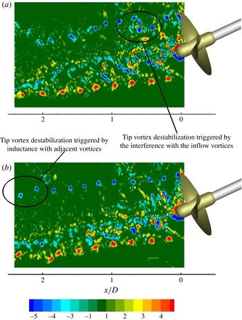
The leeward and windward portions of the wake manifest a different behaviour for propeller inclinations larger than $\unicode[STIX]{x1D6FC}=7.5^{\circ }$ . In particular, two mechanisms drive the tip vortex instability on the leeward side: (i) the reversed hydrodynamic pitch of the blade wake, which delays the spiral-to-spiral interaction, as proved by the existence of isolated (stable) tip vortices for a larger distance when the angle of attack is increased to $\unicode[STIX]{x1D6FC}=15^{\circ }$ and $\unicode[STIX]{x1D6FC}=22.5^{\circ }$ (dashed red line in figure 29 and of figure 30 b), and (ii) the interaction with the inflow eddies, which has a destabilizing effect on the tip vortices, increasing their spatial fluctuations (solid red line in figure 29 and figure 30 a). The two phase-locked snapshots reported in figure 30 for $\unicode[STIX]{x1D6FC}=22.5^{\circ }$ show how the perturbation from the inflow vortices modifies the ‘natural’ evolution of the tip vortices, shifting the instability inception from $x\cong 2D$ to $x\cong 0.75D$ .

A more in-depth analysis based on the snapshots of the out-of-plane vorticity seems to indicate an intermittent nature of the vortex shedding from the inflow and, consequently, an equally intermittent destabilizing action on the tip vortices. Conversely, when the destabilizing action of the inflow vortices is not effective, tip vortices ‘naturally’ undergo a mutual-inductance instability whose inception is delayed due to the aforementioned downstream shift of the spiral-to-spiral interaction, as shown by the dashed line in figure 29.

In contrast, on the windward side, the inception position of the tip vortex instability does not seem to manifest a notable dependence on propeller inclination.

Figure 28.

Iso-lines of regions with a positive second invariant of the phase-locked averaged velocity gradient ( $\unicode[STIX]{x1D735}u$ ) and positions of the tip vortex centroids relative to four blade passages: first blade passage (coloured in black), second blade passage (coloured in red), third blade passage (coloured in blue), fourth blade passage (coloured in orange).

Figure 29.

Locus of tip vortex instability inception ( $x^{\ast }/D$ ) versus propeller inclination ( $\unicode[STIX]{x1D6FC}$ ). Dashed line shows the inception position of the mutual-inductance instability on the leeward side for $\unicode[STIX]{x1D6FC}>7.5^{\circ }$ .

Figure 30.

Instability mechanisms for $\unicode[STIX]{x1D6FC}=22.5^{\circ }$ : tip vortex destabilization initiated by the inflow vortex perturbation (a), tip vortex destabilization initiated by mutual inductance (b). Contour plots show the instantaneous normalized out-of-plane vorticity ( $\unicode[STIX]{x1D714}_{y}D/U_{tip}$ ).

Propeller wake instability does not seem to be significantly affected by the interference between the tip vortices and the secondary vorticity generated by shear at the boundary of the propeller slipstream (see Di Mascio et al. (Reference Di Mascio, Muscari and Dubbioso2015) for a detailed explanation of the generation mechanism of the secondary vortex system). In fact, the destructive action that the secondary vorticity should exert on the propeller wake by progressive weakening of the tip vortices before the pairing process gets underway, as reported in Di Mascio et al. (Reference Di Mascio, Muscari and Dubbioso2015), does not seem to be evident in the current experimental results, as proved by the approximately constant strength of the tip vortices with distance along the wake when the propeller operates in straight and $22.5^{\circ }$ inclined flow conditions (figure 31).

In particular, the tip vortex strength does not seem to manifest the abrupt decay documented in Di Mascio et al. (Reference Di Mascio, Muscari and Dubbioso2015) for the same propeller at nearly the same operating conditions (i.e. $20^{\circ }$ propeller inclination against $22.5^{\circ }$ and $J=0.71\cos (20)=0.667$ against 0.67), as emerges by comparing the numerical and experimental results in figure 31. On the contrary, tip vortices preserve their coherence at a distance where the unwinding process exerted by the secondary vortices should have been completed with the generation of smaller structures, according to the numerical results. Therefore, the experimental results might seem to indicate that the unwinding process may occur more downstream and may not anticipate the pairing mechanism when the propeller operates at moderate/low loading rates. On the other hand, it should be said that the availability of only one component of the vorticity in the experiments and the planar nature of the measurement technique do not allow one either to perform an accurate quantitative analysis of the tip vortex intensity versus distance or to resolve the topology of the secondary vortices. This information would have better clarified the effect of secondary vorticity in the dynamics of the tip vortex system and the validity of the above conjecture.

The interference of the junction and the tip vortices do not seem to play a noteworthy effect in the mechanism of instability inception. In fact, the windward portion of the tip vortex system destabilizes at approximately the same position regardless of the propeller inclination, unlike the increasingly stronger intensity of the junction vortices and the different abscissa at which they interfere with the tip vortices when the angle of attack is increased (see figure 28).

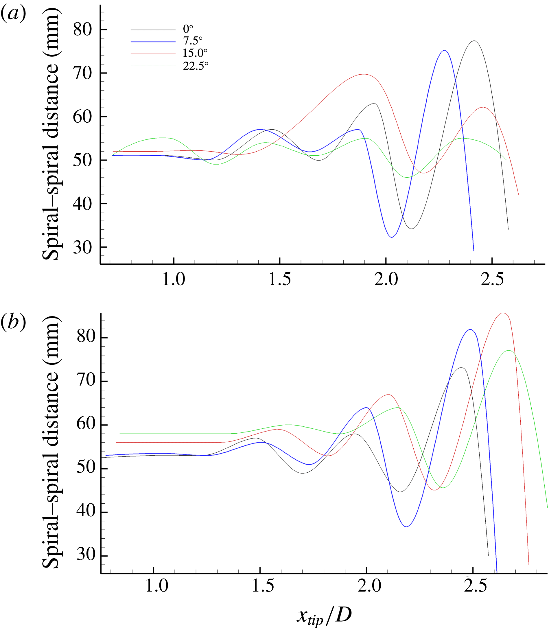
Figure 32 shows the variation of the distance between adjacent tip vortices versus the distance from the propeller and the inclination angle. The vortex-to-vortex distance initially assumes a constant value as long as the wake remains stable, and then starts to oscillate due to the mutual inductance and pairing between adjacent tip vortices, i.e. the vortex-to-vortex distance is minimum between interfering vortices and is maximum between vortices belonging to different pairs. The envelopes of the oscillation peaks show diverging profiles consistent with the tendency of adjacent tip vortices to mutually attract and pair, as documented in Felli et al. (Reference Felli, Camussi and Di Felice2011).

Figure 31.

Effect of secondary vorticity on the dynamics of the tip vortices. Numerical results by Di Mascio et al. (Reference Di Mascio, Muscari and Dubbioso2015) (a,b) (i.e. second invariant of the velocity gradient for $\unicode[STIX]{x1D6FC}=20^{\circ }$ and $J=0.667$ ), experimental results for $\unicode[STIX]{x1D6FC}=22.5^{\circ }$ (c,d) and for $\unicode[STIX]{x1D6FC}=0^{\circ }$ (e,f) (instantaneous normalized out-of-plane vorticity). Black and red arrows indicate corresponding tip vortices on the windward (a,c,e) and leeward (b,d,f) sides.

In the near field, the trend of the vortex-to-vortex distance is to increase with the inclination angle on the windward side, whereas it seems to be weakly influenced by the propeller inclination on the leeward side. No substantial differences are observed in the vortex-to-vortex distance measured on the leeward and windward sides of the wake for $\unicode[STIX]{x1D6FC}=0^{\circ }$ and $\unicode[STIX]{x1D6FC}=7.5^{\circ }$ . In contrast, a different behaviour is observed when the inclination angle is increased further, involving adjacent tip vortex traces being separated by a wider distance in the windward region. This effect is probably ascribable to the slightly convex (concave) curvature of the leeward (windward) portions of the wake stream tube that implies a local compression (stretching) of the helical geometry of the tip vortices, thus reducing (increasing) their distance.

Figure 32.

Streamwise evolution of the distance between adjacent tip vortices for $\unicode[STIX]{x1D6FC}=0^{\circ }$ , $\unicode[STIX]{x1D6FC}=7.5^{\circ }$ , $\unicode[STIX]{x1D6FC}=15^{\circ }$ and $\unicode[STIX]{x1D6FC}=22.5^{\circ }$ . Graphs refer to the leeward (a) and to the windward (b) sides of the wake.

A complementary tool to investigate the propeller wake behaviour in oblique flow conditions is given by the analysis of the second-order statistical estimators, here represented by the RMS of the out-of-plane component of the vorticity (figure 33) and by the $u^{\prime }w^{\prime }$ component of the Reynolds stresses (figure 34).

Vorticity fluctuations show an evident asymmetric behaviour on the windward and leeward side of the wake when the inclination angle is increased. The difference involves a faster decay and diffusion of the RMS peaks in the leeward portion of the wake, which is mainly due to the locally larger wandering of the tip vortices. A similar behaviour has been observed for a wind turbine by Bastankhah & Porté-Agel (Reference Bastankhah and Porté-Agel2017), who associated the smoothing effect on the phase-averaged contours of the tip vortex traces with random fluctuations of the vortices around their statistically averaged positions. Further evidence of this behaviour comes from the contour plots of the out-of-plane vorticity snapshots (figures 19 and 20) which show that: (i) the nearly constant intensity of the vorticity peaks along the wake excludes any significant mechanism of vorticity diffusion in the vortex core, (ii) the amplitude of the wandering region of the tip vortices is larger on the leeward side than on the windward side and the difference increases with the inclination angle. Analogous explanations can be applied to the progressive decay and enlargement of the RMS trace associated with the tip vortices in the downstream direction.

Figure 33.

Phase-locked evolution of the out-of-plane vorticity RMS $\big(\sqrt{\langle \unicode[STIX]{x1D714}_{y}^{\prime 2}\rangle }D/U_{tip}\big)$ for $\unicode[STIX]{x1D6FC}=0^{\circ }$ , $\unicode[STIX]{x1D6FC}=7.5^{\circ }$ , $\unicode[STIX]{x1D6FC}=15^{\circ }$ , $\unicode[STIX]{x1D6FC}=22.5^{\circ }$ (from a to d).

Figure 34.

Phase-locked evolution of the $u^{\prime }w^{\prime }$ component of the Reynolds stresses ( $\sqrt{\langle u^{\prime }w^{\prime }\rangle }/U_{tip}$ ) for $\unicode[STIX]{x1D6FC}=0^{\circ }$ , $\unicode[STIX]{x1D6FC}=7.5^{\circ }$ , $\unicode[STIX]{x1D6FC}=15^{\circ }$ , $\unicode[STIX]{x1D6FC}=22.5^{\circ }$ (from a to d).

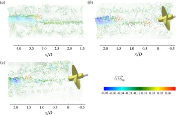
The distribution of the Reynolds stresses exhibits an abrupt sign reversal along the trace of the hub vortex at approximately $x=3.6D$ , $x=2D$ , $x=1.6D$ , when the propeller operates in axisymmetric inflow and when it is inclined by $7.5^{\circ }$ and $15^{\circ }$ , respectively (figure 34). This behaviour seems to have a relation to the inception of the hub vortex instability considering that the sign change in the Reynolds stresses is a recurrent feature in the instability of coherent structures (Mankbadi Reference Mankbadi1994), it being indicative of a reversal in the direction of the energy transfer between a vortical structure and the mean flow (Zaman & Hussain Reference Zaman and Hussain1985). Furthermore, the sign reversal of the instantaneous value of $u^{\prime }w^{\prime }$ is always associated with an abrupt variation of the velocity fluctuations which might be interpreted as a distinguishing feature of the hub vortex destabilization (see vector plots of figure 35). Unfortunately, the availability of the instantaneous velocity field only in a relatively limited flow region, along with the gradual growth of the amplitude of the hub vortex deformation for this propeller at this loading regime (see figure 12 in Felli et al. (Reference Felli, Camussi and Di Felice2011)), do not allow one to resolve any significant shape deformation of the vortex trace which might be appreciable further downstream. Accessibility to instantaneous flow-field data over a larger wake extent, possibly combined with detailed flow measurements in transversal sections of the wake and time-resolved visualizations, might clarify the conjecture of the hub vortex instability inception behind the sign reversal of the associated Reynolds stress distribution.

Figure 35.

Vector plots of the instantaneous streamwise velocity fields subtracted by the mean velocity for $\unicode[STIX]{x1D6FC}=0^{\circ }$ (a), $\unicode[STIX]{x1D6FC}=7.5^{\circ }$ (b) and $\unicode[STIX]{x1D6FC}=15^{\circ }$ (c). Vectors are coloured with the instantaneous component of the Reynolds stresses ( $u^{\prime }w^{\prime }/U_{tip}^{2}$ ).

6 Summary and conclusions

The underlying mechanisms of propeller wake behaviour in oblique flow conditions are investigated in the present study by detailed flow measurements using particle image velocimetry (PIV). The study consisted of a systematic comparison of the morphological and kinematic characteristics of the propeller wake in axisymmetric and oblique flow conditions, under three different inclination angles and for a wide spatial extent of the propeller wake covering the near-field, transition and far-field regions up to $4.5D$ from the propeller disk. To this end, a multicamera recoding system with three cameras arranged side by side was used to simultaneously acquire the wake flow over such a large spatial extent. The study was based on analysis of the instantaneous and phase-locked averaged wake flow characteristics.

The dynamics of the propeller vortical systems in oblique flow shows a markedly different behaviour with respect to the axisymmetric condition, which is accentuated with increasing propeller inclination. The differences are basically the consequence of two major factors: wake stream-tube misalignment with the main flow, which affects the morphology of vortical systems and influences their interaction mechanisms, and the presence of a main flow component on the propeller plane, which causes variable blade loading and circulation along the azimuth. In particular, the major effects of oblique flow operation can be summarized as follows.

(i) The propeller stream tube undergoes a deformation under the effect of the main flow with a mechanism similar to a jet in cross-flow. In particular, the contrasting effect of the main flow on the wake penetration becomes stronger and stronger with increasing propeller inclination and is manifested within a few diameters downstream of the propeller plane.
(ii) The tip vortices and the hub vortex are deflected at approximately the same rate. It follows that the wake stream tube preserves the cross-sectional shape during the deformation. The same deflection is ‘asymptotically’ assumed by the blade junction vortices, whose trajectory is obstructed by interference with the tip vortices. The interference initiates on the leeward side, where the deflection angles of tip and junction vortices have opposite signs, and takes place closer and closer to the propeller plane when increasing the inclination angle.
(iii) The bending characteristics of the blade wake show a markedly asymmetric behaviour in the leeward and windward regions, and are significantly dependent on the inclination angle. The asymmetry is accentuated with increasing propeller inclination and involves the different position at which the ‘spiral-to-spiral’ interference is manifested. In particular, the ‘reversed’ hydrodynamic pitch of the inboard sections of the blade wake on the leeward side has a retardant effect on the spiral-to-spiral interference, shifting downstream the interference between the tip vortex and the blade wake of adjacent spirals.
(iv) Tip vortex mutual-inductance instability initiates on the leeward side and moves further upstream with increasing propeller inclination for small angles (i.e. $\unicode[STIX]{x1D6FC}\leqslant 7.5^{\circ }$ ). Increasing the propeller inclination further, the instability inception is shifted downstream due to the retardant effect exerted by the ‘reversed’ hydrodynamic pitch of the blade wake on the spiral-to-spiral interference. The perturbation of the inflow vortices originating from the shaft is a further effect that ‘intermittently’ destabilizes the tip vortex branches on the leeward side within a radial distance from the propeller plane.
(v) The secondary vorticity generated by shear at the boundary of the propeller slipstream seems not to have a noteworthy effect on the tip vortices, which preserve their coherence at a distance where the unwinding process should have been completed with the generation of smaller structures, according to Di Mascio et al. (Reference Di Mascio, Muscari and Dubbioso2015). Therefore, the experimental results seem to indicate that the unwinding process may not anticipate the pairing mechanism when the propeller operates at moderate/low loading rates. Analogously, the perturbation of the junction vortices does not seem to have an effect on the wake instability.

In conclusion, the proposed experimental approach has provided new quantitative and qualitative information about the wake dynamics of a propeller operating in oblique flow. Nevertheless, some aspects related to the mechanisms of wake destabilization are still not fully understood and, therefore, deserve further investigations. In particular, these concern the role of the secondary vorticity sheet and the underlying inception mechanism of the hub vortex instability. To this end, a range of other investigation and analysis methodologies can be applied, including volumetric flow measurements, pressure fluctuation measurements and time-resolved visualizations.

Acknowledgements

This work was supported by the U.S. Office of Naval Research (ONR) under NICOP grant N62909-15-1-2007, ‘Experimental Study of Hydrodynamics and Hydroacoustics of Marine Propellers’ through Drs K.-H. Kim (ONR HQs), A. Salahuddin (ONR Global) and W.-M. Lin (formerly ONR Global). We gratefully acknowledge their support.

References

Adrian, R. J. & Westerweel, J. 2011 Particle Image Velocimetry. Cambridge University Press.Google Scholar

Aeschlimann, V., Beaulieu, S., Houde, S., Dan Ciocan, G. & Deschenes, C. 2013 Inter-blade flow analysis of a propeller turbine runner using stereoscopic PIV. Eur. J. Mech. (B/Fluids) 42, 121–128.CrossRef Google Scholar

Atsavapranee, P., Miller, R., Day, C., Klamo, J. & Fry, D. 2010 Steady-turning experiments and RANS simulations on a surface combatant hull form (model #5617). In Proceedings of 28th Symposium on Naval Hydrodynamics, Pasadena, CA, Office of Naval Research.Google Scholar

Bastankhah, M. & Porté-Agel, F. 2016 Experimental and theoretical study of wind turbine wakes in yawed conditions. J. Fluid Mech. 806, 506–541.Google Scholar

Bastankhah, M. & Porté-Agel, F. 2017 Wind tunnel study of the wind turbine interaction with a boundary-layer flow: upwind region, turbine performance, and wake region. Phys. Fluids 29 (6), 065015.Google Scholar

Budich, B., Schmidt, S. J. & Adams, N. A. 2015 Numerical simulation of cavitating ship propeller flow and assessment of erosion aggressiveness. In 6th Conference on Computational Methods in Marine Engineering (Marine 2015), Rome, Italy, ECCOMAS.Google Scholar

Bhagwat, M. J. & Leishman, J. G. 2000 Stability analysis of helicopter rotor wakes in axial flight. J. Am. Helicopter Assoc. 45, 165–178.CrossRef Google Scholar

Carlton, J. 2012 Marine Propellers and Propulsion. Elsevier.Google Scholar

Chamorro, L., Hill, C., Morton, S., Ellis, C., Arndt, R. E. & Sotiropoulos, F. 2013 On the interaction between a turbulent open channel flow and an axial-flow turbine. J. Fluid Mech. 716, 658–670.Google Scholar

Chesnakas, C. & Jessup, S. 1998 Experimental characterization of propeller tip flow. In Proceedings of the 22nd Symposium on Naval Hydrodynamics, Washington, Office of Naval Research.Google Scholar

Chih-Chung, Y.1990 The effects of forebody strakes on asymmetric vortices on a vertically launched missile. PhD thesis, Naval Postgraduate School, Monterey.Google Scholar

Cumpsty, N. A. & Lowrie, B. W. 1974 The cause of tone generation by aeroengine fans at high subsonic speeds and the effect of forward speed. J. Engng Power 96 (3), 228–234.Google Scholar

Del Pino, C., Parras, L., Felli, M. & Fernandez-Feria, R. 2011 Structure of trailing vortices: comparison between particle image velocimetry measurements and theoretical models. Phys. Fluids 23 (1), 013602.CrossRef Google Scholar

Di Felice, F., Di Florio, D., Felli, M. & Romano, G. P. 2004 Experimental investigation of the propeller wake at different loading conditions by particle image velocimetry. J. Ship Res. 48 (2), 168–190.CrossRef Google Scholar

Di Mascio, A., Muscari, R. & Dubbioso, G. 2015 On the wake dynamics of a propeller operating in drift. J. Fluid Mech. 754, 263–307.CrossRef Google Scholar

Dubbioso, G., Muscari, R. & Di Mascio, A. 2013 Analysis of the performance of a marine propeller in oblique flow. Comput. Fluids 75, 86–102.Google Scholar

Dubbioso, G., Muscari, R. & Di Mascio, A. 2014 Analysis of a marine propeller operating in oblique flow. Part 2: very high incidence angles. Comput. Fluids 92, 56–81.CrossRef Google Scholar

Felli, M., Camussi, R. & Di Felice, F. 2011 Mechanisms of evolution of the propeller wake in the transition and far fields. J. Fluid Mech. 682, 1–17.Google Scholar

Felli, M. & Di Felice, F. 2005 Propeller wake analysis in not uniform inflow by LDV phase sampling techniques. J. Marine Sci. Technol. 10 (4), 159–172.Google Scholar

Felli, M., Di Felice, F., Guj, G. & Camussi, R. 2006 Analysis of the propeller wake evolution by pressure and velocity phase measurements. Exp. Fluids 1, 1–11.Google Scholar

Felli, M., Guj, G. & Camussi, R. 2008 Effect of the number of blades on propeller wake evolution. Exp. Fluids 44, 409–418.Google Scholar

Frandsen, S. & Thøgersen, M. L. 1999 Integrated fatigue loading for wind turbines in wind farms by combining ambient turbulence and wakes. Wind Engng 23 (6), 327–339.Google Scholar

Gand, F., Deck, S., Brunet, V. & Sagaut, P. 2010 Flow dynamics past a simplified wing body junction. Phys. Fluids 22, 115111.CrossRef Google Scholar

Grant, I. & Parkin, P. 2000 A DPIV study of the trailing vortex elements from the blades of a horizontal axis wind turbine in yaw. Exp. Fluids 28 (4), 368–376.Google Scholar

Grant, I., Parkin, P. & Wang, X. 1997 Optical vortex tracking studies of a horizontal axis wind turbine in yaw using laser-sheet, flow visualisation. Exp. Fluids 23 (6), 513–519.Google Scholar

Gupta, B. P. & Loewy, R. G. 1974 Theoretical analysis of the aerodynamic stability of multiple, interdigitated helical vortices. AIAA J. 12, 1381–1387.Google Scholar

Haans, W., Sant, T., Van Kuik, G. & Van Bussel, G. 2005 Measurement and modelling of tip vortex paths in the wake of a HAWT under yawed flow conditions. In 43th AIAA Aerospace Sciences Meeting and Exhibit, pp. 136–145. AIAA.Google Scholar

Haans, W., Van Kuik, G. & Van Bussel, G. J. W. 2007 Experimentally observed effects of yaw misalignment on the inflow in the rotor plane. J. Phys.: Conf. Ser. 75, 012012.Google Scholar

Hunt, J. C. R., Wray, A. A. & Moin, P.1988 Eddies, stream, and convergence zones in turbulent flows. Center for Turbulence Research Report CTR-S88, pp. 193–208.Google Scholar

Huyer, S. A. & Snarski, S. R. 2003 Analysis of a turbulent propeller inflow. Trans. ASME J. Fluids Engng 125 (3), 533–542.Google Scholar

Jessup, S. D.1989 An experimental investigation of viscous aspects of propeller blade flow. PhD thesis, The Catholic University of America, Washington DC, 1989.Google Scholar

Jiménez, Á., Crespo, A. & Migoya, E. 2010 Application of a LES technique to characterize the wake deflection of a wind turbine in yaw. Wind Energy 13 (6), 559–572.Google Scholar

Joukowsky, N. E. 1912 Vortex theory of screw propeller, I–IV. Trudy Otdeleniya Fizicheskikh Nauk Obshchestva Lubitelei Estestvoznaniya: part I 16 (1), 1–31.Google Scholar

Kerwin, J. E. 1986 Marine propellers. Annu. Rev. Fluid Mech. 18, 367–403.CrossRef Google Scholar

Kumar, P. & Mahesh, K. 2017 Large eddy simulation of propeller wake instabilities. J. Fluid Mech. 814, 361–396.Google Scholar

Landgrebe, A. J. 1972 The wake geometry of a hovering rotor and its influence on rotor performance. J. Am. Hel. Soc. 17 (4), 3–15.Google Scholar

Leishmann, J. G. 2006 Principles of Helicopter Aerodynamics. Wiley.Google Scholar

Leung, Y. C. & Yang, Y. 2012 Wind energy development and its environmental impact: a review. Renew. Sustainable Energy Rev. 16, 1031–1039.Google Scholar

Levy, H. & Forsdyke, A. G. 1928 The steady motion and stability of a helical vortex. Proc. R. Soc. Lond. A 120, 670–690.Google Scholar

Mahesh, K. 2013 The interaction of jets with crossflow. Annu. Rev. Fluid Mech. 45, 379–407.Google Scholar

Mankbadi, R. 1994 Transition, Turbulence and Noise: Theory and Applications for Scientists and Engineers. Springer Science and Business Media.Google Scholar

Marshall, J. S. 2003 Wake dynamics of yawed cylinders. Trans. ASME J. Fluids Engng 125, 97–103.CrossRef Google Scholar

Micallef, D. & Sant, T. 2016 A review of wind turbine yaw aerodynamics. In Wind Turbines – Design, Control and Applications (ed. Aissaoui, A. G. & Tahour, A.), chap. 2, ISBN 978-953-51-2496-2.Google Scholar

Micallef, D., Bussel, G., Ferreira, C. S. & Sant, T. 2013 An investigation of radial velocities for a horizontal axis wind turbine in axial and yawed flows. Wind Energy 16 (4), 529–544.Google Scholar

Okulov, V. L. 2004 On the stability of multiple helical vortices. J. Fluid Mech. 521, 319–342.Google Scholar

Okulov, V. L. & Sørensen, J. N. 2007 Stability of helical tip vortices in rotor far wake. J. Fluid Mech. 576, 1–25.CrossRef Google Scholar

Rajaratnam, N. 1976 Turbulent Jets. Elsevier.Google Scholar

Robison, R. A. V. & Peake, N. 2014 Noise generation by turbulence–propeller interaction in asymmetric flow. J. Fluid Mech. 758, 121–149.Google Scholar

Salvatore, F., Pereira, F., Felli, M., Calcagni, D. & Di Felice, F.2006 Description of the INSEAN E779A propeller experimental dataset. INSEAN Tech. Rep. 2006-085.Google Scholar

Scarano, F. 2002 Iterative image deformation methods in PIV. Meas. Sci. Technol. 13, 1–19.Google Scholar

Simpson, R. 2001 Junction flows. Annu. Rev. Fluid Mech. 33, 415–443.CrossRef Google Scholar

Stevens, J. A. M. & Meneveau, C. 2014 Temporal structure of aggregate power fluctuations in large-eddy simulations of extended wind-farms. J. Renew. Sustainable Energy 6, 043102.Google Scholar

Stevens, J. A. M. & Meneveau, C. 2017 Flow structure and turbulence in wind farms. Annu. Rev. Fluid Mech. 49, 311–339.Google Scholar

Surry, J. & Surry, D.1967 The effect of inclination on the Strouhal number and other wake properties of circular cylinders at subcritical Reynolds numbers. Tech. Rep., University of Toronto, Institute for Aerospace Studies.Google Scholar

Thakur, A., Liu, X. & Marshall, J. S. 2004 Wake flow of single and multiple yawed cylinders. Trans. ASME J. Fluids Engng 126, 861–870.CrossRef Google Scholar

Varshney, K. 2013 Characteristics of helical tip vortices in a wind turbine near wake. Theor. Appl. Climatol. 111, 427–435.Google Scholar

Vermeer, L. J., Sorensen, J. N. & Crespo, A. 2003 Wind turbine wake aerodynamics. Prog. Aerosp. Sci. 39, 467–510.CrossRef Google Scholar

Viviani, M., Podenzana Bonvino, C., Mauro, S., Cerruti, M., Guadalupi, D. & Menna, A. 2007 Analysis of asymmetrical shaft power increase during tight manoeuvre. In 9th International Conference on Fast Sea Transportation (FAST 2007), Shanghai, China. GICAN.Google Scholar

Walther, J. H., Guénot, M., Machefaux, E., Rasmussen, J. T., Chatelain, P., Okulov, V. L., Sørensen, J. N., Bergdorf, M. & Koumoutsakos, P. 2007 A numerical study of the stability of helical vortices using vortex methods. J. Phys.: Conf. Ser. 75, 012034.Google Scholar

Westerweel, J. & Scarano, F. 2005 Universal outlier detection for PIV data. Exp. Fluids 39, 1096–1100.CrossRef Google Scholar

Widnall, S. E. 1972 The stability of helical vortex filament. J. Fluid Mech. 54, 641–663.Google Scholar

Wood, D. H. & Boersma, J. 2001 On the motion of multiple helical vortices. J. Fluid Mech. 447, 149–171.Google Scholar

Zaman, K. B. M. Q. & Hussain, A. K. M. F. 1985 Natural large-scale structures in the axisymmetric mixing layer. J. Fluid Mech. 138, 325–351.Google Scholar

Figure 1.Sketch of the vortical systems in the wake of a propeller operating in a non-uniform inflow.

Figure 2.Wake perturbation effects: $P$-factor (a), onset flow effect (b), main flow effect (c). The contour plot in (c) shows the normalized phase-locked averaged out-of-plane component of the vorticity ($\langle \unicode[STIX]{x1D714}_{y}\rangle D/U_{tip}$, where $U_{tip}=n\unicode[STIX]{x03C0}D=6.75~\text{m}~\text{s}^{-1}$, $n=$ propeller rotational speed and $D=$ propeller diameter). White lines represent the boundary of the propeller stream tube.

Figure 3.(a) Reference frames. (b) The contour plot shows the normalized phase-locked averaged out-of-plane component of the vorticity ($\langle \unicode[STIX]{x1D714}_{y}\rangle D/U_{tip}$); $\unicode[STIX]{x1D6FD}$ represents the pitch angle of the blade wake.

Figure 4.CNR INSEAN E779A propeller.

Figure 5.Propeller mounting: $h$ and $\unicode[STIX]{x1D6FC}$ represent the submersion and the inclination of the propeller, respectively.

Table 1.Geometrical characteristics of the CNR INSEAN E779A propeller.

Figure 6.Top and side views of the PIV experimental set-up.

Figure 7.Field of view of the multicamera system used for the PIV measurements (white: camera field of view in the upstream region, black: camera field of view in the downstream region). Contour plots show the normalized phase-locked averaged out-of-plane component of the vorticity ($\langle \unicode[STIX]{x1D714}_{y}\rangle D/U_{tip}$).

Figure 8.PIV measurement convergence analysis. Red line represents the percentage deviation between the phase-locked averaged out-of-plane component of the vorticity calculated over # samples (with # ranging from 0 to 1000) ($\langle \unicode[STIX]{x1D714}\rangle _{\#}$) and over 1000 samples ($\langle \unicode[STIX]{x1D714}\rangle _{1000}$). Black line represents the percentage deviation between the phase-locked RMS of the out-of-plane vorticity calculated over # samples ($\langle \sqrt{\unicode[STIX]{x1D714}^{\prime 2}}\rangle _{\#}$) and over 1000 samples ($\langle \sqrt{\unicode[STIX]{x1D714}^{\prime 2}}\rangle _{1000}$).

Figure 9.Propeller onset flow. Contours of the normalized out-of-plane vorticity $\unicode[STIX]{x1D714}_{y}D/U_{tip}$ at a given instant for $\unicode[STIX]{x1D6FC}=0^{\circ }$, $\unicode[STIX]{x1D6FC}=7.5^{\circ }$, $\unicode[STIX]{x1D6FC}=15^{\circ }$, $\unicode[STIX]{x1D6FC}=22.5^{\circ }$.

Figure 10.Propeller onset flow. Contours of the normalized mean out-of-plane vorticity $\bar{\unicode[STIX]{x1D714}}_{y}D/U_{tip}$ for $\unicode[STIX]{x1D6FC}=0^{\circ }$, $\unicode[STIX]{x1D6FC}=7.5^{\circ }$, $\unicode[STIX]{x1D6FC}=15^{\circ }$, $\unicode[STIX]{x1D6FC}=22.5^{\circ }$.

Figure 11.Propeller onset flow. Contours of the normalized RMS of the out-of-plane vorticity $\sqrt{\overline{{\unicode[STIX]{x1D714}^{\prime }}_{y}^{2}}}D/U_{tip}$ for $\unicode[STIX]{x1D6FC}=0^{\circ }$, $\unicode[STIX]{x1D6FC}=7.5^{\circ }$, $\unicode[STIX]{x1D6FC}=15^{\circ }$, $\unicode[STIX]{x1D6FC}=22.5^{\circ }$.

Figure 12.Evolution of the normalized mean streamwise velocity ($\bar{u}/U_{\infty }$) (a,c,e,g) and of the turbulent intensity ($\unicode[STIX]{x1D70E}_{x}/U_{\infty }$) (b,d,f,h) for $\unicode[STIX]{x1D6FC}=0^{\circ }$ (a,b), $\unicode[STIX]{x1D6FC}=7.5^{\circ }$ (c,d), $\unicode[STIX]{x1D6FC}=15^{\circ }$ (e,f) and $\unicode[STIX]{x1D6FC}=22.5^{\circ }$ (g,h). Dashed lines indicate the locations where velocity profiles of figures 14 and 15 are extracted. The black dashed-dot lines represent the wake-centre trajectory in the measurement plane obtained from the velocity profiles of figure 14 by measuring the distance between the positions where the flow velocity exceeds the free-stream velocity by 5 %.

Figure 13.Snapshots of the normalized streamwise velocity ($u/U_{\infty }$) at a given propeller phase (i.e. the two snapshots are relative to two instants at the same propeller position) for $\unicode[STIX]{x1D6FC}=0^{\circ }$ (a,c), $\unicode[STIX]{x1D6FC}=7.5^{\circ }$ (b,d), $\unicode[STIX]{x1D6FC}=15^{\circ }$ (e,g) and $\unicode[STIX]{x1D6FC}=22.5^{\circ }$ (f,h).

Figure 14.Profiles of the normalized streamwise velocity ($\bar{u}/U_{\infty }$) downstream of the propeller for $\unicode[STIX]{x1D6FC}=0^{\circ }$, $7.5^{\circ }$, $15^{\circ }$ and $22.5^{\circ }$ (from a to d respectively) for different downstream positions. For each position, $\bar{u}/U_{\infty }=1$ on the vertical thick black line. The width of the grid squares corresponds to $0.088U_{\infty }$.

Figure 15.Profiles of the turbulent intensity ($I_{x}$) downstream of the propeller for $\unicode[STIX]{x1D6FC}=0^{\circ }$, $7.5^{\circ }$, $15^{\circ }$ and $22.5^{\circ }$ (from a to d respectively) for different downstream positions. For each position, $I_{x}=I_{\infty }$ ($I_{\infty }=$ facility turbulence, see § 3.1) on the vertical thick black line. The width of the grid squares corresponds to $0.088U_{\infty }$.

Figure 16.Evolution of the maximum of the mean streamwise velocity $\bar{u}_{max}/U_{\infty }$ (a) and of the velocity gap between maximum and minimum values of the mean streamwise velocity $(\bar{u}_{max}-\bar{u}_{min})/U_{\infty }$ (b) for $\unicode[STIX]{x1D6FC}=0^{\circ }$, $\unicode[STIX]{x1D6FC}=7.5^{\circ }$, $\unicode[STIX]{x1D6FC}=15^{\circ }$, $\unicode[STIX]{x1D6FC}=22.5^{\circ }$. Symbols on the top of the figure are coloured in red when the velocity maximum is located on the leeward side. Linear fits are used to estimate the position where the velocity gap is zero.

Figure 17.Sketch of the vortex systems in the wake of a propeller operating in inclined flow condition. Contour plot shows the normalized phase-locked averaged out-of-plane component of the vorticity $\langle \unicode[STIX]{x1D714}_{y}\rangle D/U_{tip}$.

Figure 18.Phase-locked evolution of the normalized out-of-plane vorticity ($\langle \unicode[STIX]{x1D714}_{y}\rangle D/U_{tip}$) for $\unicode[STIX]{x1D6FC}=0^{\circ }$, $\unicode[STIX]{x1D6FC}=7.5^{\circ }$, $\unicode[STIX]{x1D6FC}=15^{\circ }$, $\unicode[STIX]{x1D6FC}=22.5^{\circ }$ (from a to d).

Figure 19.Snapshots of the normalized out-of-plane vorticity ($\unicode[STIX]{x1D714}_{y}D/U_{tip}$) at a given propeller phase (i.e. the four snapshots are relative to four instants at the same propeller position) for $\unicode[STIX]{x1D6FC}=0^{\circ }$ (a,c,e,g) and $\unicode[STIX]{x1D6FC}=7.5^{\circ }$ (b,d,f,h).

Figure 20.Snapshots of the normalized out-of-plane vorticity ($\unicode[STIX]{x1D714}_{y}D/U_{tip}$) at a given propeller phase (i.e. the four snapshots are relative to four instants at the same propeller position) for $\unicode[STIX]{x1D6FC}=15^{\circ }$ (a,c,e,g) and $\unicode[STIX]{x1D6FC}=22.5^{\circ }$ (b,d,f,h).

Figure 21.Leeward and windward root vortex traces for the propeller inclination $\unicode[STIX]{x1D6FC}=22.5^{\circ }$. Iso-contours describe the phase-locked normalized out-of-plane vorticity ($\langle \unicode[STIX]{x1D714}_{y}\rangle D/U_{tip}$).

Figure 22.Contour lines of the tip vortex traces during a complete propeller revolution for $\unicode[STIX]{x1D6FC}=0^{\circ }$, $\unicode[STIX]{x1D6FC}=7.5^{\circ }$, $\unicode[STIX]{x1D6FC}=15^{\circ }$ and $\unicode[STIX]{x1D6FC}=22.5^{\circ }$. Tip vortex traces are represented after a rotation by the inverse of the inclination angle in the vertical plane. Dashed lines are extrapolated from the envelope profiles of the tip vortices (solid lines) using a linear regression fit. Labels indicate the slopes of the extrapolated lines.

Figure 23.Propeller wake penetration versus inclination angle. The wake deflection angle for a given propeller inclination is represented by the slope of the linear regression fit of the tip vortex envelope profiles, as reported in figure 22.

Figure 24.Envelope profiles of the vortex systems in the propeller wake for $\unicode[STIX]{x1D6FC}=0^{\circ }$, $\unicode[STIX]{x1D6FC}=7.5^{\circ }$, $\unicode[STIX]{x1D6FC}=15^{\circ }$ and $\unicode[STIX]{x1D6FC}=22.5^{\circ }$. Scatter plots represent the locus of the vortex centres in the measurement plane. The slopes of the envelope profiles (in magnitude) are indicated by labels.

Figure 25.Streamwise evolution of the pitch angle of the blade wake ($\unicode[STIX]{x1D6FD}$) for $\unicode[STIX]{x1D6FC}=0^{\circ }$, $\unicode[STIX]{x1D6FC}=7.5^{\circ }$, $\unicode[STIX]{x1D6FC}=15^{\circ }$ and $\unicode[STIX]{x1D6FC}=22.5^{\circ }$. Leeward region (a) and windward region (b). The pitch angle $\unicode[STIX]{x1D6FD}$ is estimated from the slope of the linear regression of the locations of the vorticity peaks along the blade wake trace in the measurement plane.

Figure 26.Hydrodynamic pitch characteristics of the blade trailing wake ($\unicode[STIX]{x1D6FD}$) for $\unicode[STIX]{x1D6FC}=22.5^{\circ }$. The letter in the superscript and the number in the subscript refer to the portion of the propeller wake (i.e. $W=$ windward, $L=$ leeward) and to the ordinal of the spiral (i.e. increasing with increasing streamwise distance), respectively. Contour plot shows the normalized phase-locked RMS of the axial velocity $\sqrt{\langle u^{\prime 2}\rangle }/U_{tip}$ for $\unicode[STIX]{x1D6FC}=22.5^{\circ }$.

Figure 27.Instantaneous contour plot (a,b) and phase-locked averaged (iso-lines on the c,d) representation of the trailing wake deformation and interaction with the tip vortex. Both contours and iso-lines are coloured with the out-of-plane component of the vorticity ($\langle \unicode[STIX]{x1D714}_{y}\rangle D/U_{tip}$) for $\unicode[STIX]{x1D6FC}=0^{\circ }$ (a,c) and $\unicode[STIX]{x1D6FC}=22.5^{\circ }$ (b,d).

Figure 28.Iso-lines of regions with a positive second invariant of the phase-locked averaged velocity gradient ($\unicode[STIX]{x1D735}u$) and positions of the tip vortex centroids relative to four blade passages: first blade passage (coloured in black), second blade passage (coloured in red), third blade passage (coloured in blue), fourth blade passage (coloured in orange).

Figure 29.Locus of tip vortex instability inception ($x^{\ast }/D$) versus propeller inclination ($\unicode[STIX]{x1D6FC}$). Dashed line shows the inception position of the mutual-inductance instability on the leeward side for $\unicode[STIX]{x1D6FC}>7.5^{\circ }$.

Figure 30.Instability mechanisms for $\unicode[STIX]{x1D6FC}=22.5^{\circ }$: tip vortex destabilization initiated by the inflow vortex perturbation (a), tip vortex destabilization initiated by mutual inductance (b). Contour plots show the instantaneous normalized out-of-plane vorticity ($\unicode[STIX]{x1D714}_{y}D/U_{tip}$).

Figure 31.Effect of secondary vorticity on the dynamics of the tip vortices. Numerical results by Di Mascio et al. (2015) (a,b) (i.e. second invariant of the velocity gradient for $\unicode[STIX]{x1D6FC}=20^{\circ }$ and $J=0.667$), experimental results for $\unicode[STIX]{x1D6FC}=22.5^{\circ }$ (c,d) and for $\unicode[STIX]{x1D6FC}=0^{\circ }$ (e,f) (instantaneous normalized out-of-plane vorticity). Black and red arrows indicate corresponding tip vortices on the windward (a,c,e) and leeward (b,d,f) sides.

Figure 32.Streamwise evolution of the distance between adjacent tip vortices for $\unicode[STIX]{x1D6FC}=0^{\circ }$, $\unicode[STIX]{x1D6FC}=7.5^{\circ }$, $\unicode[STIX]{x1D6FC}=15^{\circ }$ and $\unicode[STIX]{x1D6FC}=22.5^{\circ }$. Graphs refer to the leeward (a) and to the windward (b) sides of the wake.

Figure 33.Phase-locked evolution of the out-of-plane vorticity RMS $\big(\sqrt{\langle \unicode[STIX]{x1D714}_{y}^{\prime 2}\rangle }D/U_{tip}\big)$ for $\unicode[STIX]{x1D6FC}=0^{\circ }$, $\unicode[STIX]{x1D6FC}=7.5^{\circ }$, $\unicode[STIX]{x1D6FC}=15^{\circ }$, $\unicode[STIX]{x1D6FC}=22.5^{\circ }$ (from a to d).

Figure 34.Phase-locked evolution of the $u^{\prime }w^{\prime }$ component of the Reynolds stresses ($\sqrt{\langle u^{\prime }w^{\prime }\rangle }/U_{tip}$) for $\unicode[STIX]{x1D6FC}=0^{\circ }$, $\unicode[STIX]{x1D6FC}=7.5^{\circ }$, $\unicode[STIX]{x1D6FC}=15^{\circ }$, $\unicode[STIX]{x1D6FC}=22.5^{\circ }$ (from a to d).

Figure 35.Vector plots of the instantaneous streamwise velocity fields subtracted by the mean velocity for $\unicode[STIX]{x1D6FC}=0^{\circ }$ (a), $\unicode[STIX]{x1D6FC}=7.5^{\circ }$ (b) and $\unicode[STIX]{x1D6FC}=15^{\circ }$ (c). Vectors are coloured with the instantaneous component of the Reynolds stresses ($u^{\prime }w^{\prime }/U_{tip}^{2}$).

Article contents

Propeller wake evolution mechanisms in oblique flow conditions

Abstract

JFM classification

Information

1 Introduction

2 Reference frames and dimensionless groups

3 Experimental set-up

3.1 Facility

3.2 Case study

3.3 PIV measurements

4 Test conditions

5 Results

5.1 Nominal wake flow

5.2 Mean and instantaneous flow distribution

5.3 Wake dynamics

6 Summary and conclusions

Acknowledgements

References

Save article to Kindle

Save article to Dropbox

Save article to Google Drive

Reply to: Submit a response

Your details

You have entered the maximum number of contributors

Conflicting interests