Introduction
Wireless power transfer (WPT) technologies have been applied in many fields, such as mobile phones, implantable devices, and electric vehicles, in the past few years [Reference Fan, Zhang and Zhang1, Reference Wang, Wang, Liang, Fan, Nie, Yan and Xu2]. Currently, most WPT systems are realized by using a pair of inductively coupled coils at the transmitter (Tx) and the receiver (Rx) ends, respectively. The Tx and Rx coils are tuned to resonate at the same intrinsic resonant frequency as the AC power source. The power transfer efficiency (PTE), one of the most concerned parameters of WPT systems, strongly relies on the coupling coefficient between the Tx and Rx coils. The coupling coefficient in a single Tx coil and single Rx coil scenario is determined by the size of each coil and the relative position and orientation. For example, in the applications of wireless charging for free-positioning portable consumer electronics and electric vehicles, the lateral misalignment between the Tx and Rx coils happens easily, which results in a decrease in coupling coefficient, PTE, and power delivered to the load (PDL). An effective way to prevent lateral misalignment is to enlarge the charging region by using multiple distributed Txs. Taking the original Tx as a unit, placing one or more identical Tx units next to the original one, and forming a replicable system is a convenient way to extend the charging region. However, implementing a well-designed multi-Tx system to achieve optimal efficiency and stable output power is not an easy task.
First, these identical Txs should provide synchronous current at the Tx coils to ensure maximum utilization of the transmitted energy. Currently, it is achieved by connecting multiple Txs’ power sources or coils through a wired connection [Reference Jouya and Dina3]. This obviously makes the assembly of the Txs inconvenient. For different applications requiring different numbers of Tx modules, the Tx setup needs to be customized.
Second, the current amplitude of each coil should ideally be proportional to the mutual inductance between its Tx coil and Rx coil [Reference Waters, Mahoney, Ranganathan and Smith4–Reference Chen, Cheng, Yang and Pan8]. In existing systems, customized current amplitude adjustment algorithms are developed in accordance with the monitored mutual inductance by detecting the current, voltage, or impedance information on either the Tx or Rx sides [Reference Kim and Ahn9–Reference Qiu, Zhang, Chen, Takamiya and Shi14]. Undoubtedly, additional sensing hardware, complicated software, and even wireless communication between the Tx and Rx sides are required. Fortunately, as stated in [Reference Kim, Jeon and Seo15], the multi-Tx system with identical current in each Tx coil can achieve near-optimal efficiency as long as the ratio of the minimum to the maximum mutual inductance between the Tx coil and Rx coil is more than 1/2.
Third, the impact of the mutual couplings between the Tx coils should be eliminated. The external impedance introduced by its adjacent Tx coils can result in a mismatch between the resonant frequency and operating frequency, asynchronous Tx coil current phases, and can even disrupt the zero-voltage-switching (ZVS) operation of the inverters [Reference Ahn and Hong16–Reference Huh, Park, Choi, Shin, Kim, Kim, Park, Park and Ahn21]. Different structural coils [Reference Zaheer, Hao, Covic and Kacprzak22], such as partially overlapped DD coil [Reference Liu and Zhang23], bipolar pad coil [Reference Lin, Kim, Covic and Boys24], tripolar pad coil [Reference Kim, Covic and Boys25], and other structural coils [Reference Wu, Yang, Chen, Wang, Jiang, Gao, Yan and Yu26], have been applied in multi-Tx systems to decouple Tx coils. However, in practice, even a small variation in the overlapping width between Tx coils results in nonzero coupling between Tx coils [Reference Lin, Carretero, Covic and Boys27]. Alternatively, rather than trying to eliminate these mutual couplings perfectly, the phases of the Tx coil currents are adjusted adaptively through complex algorithms [Reference Li, Mai, Lu, Lin, Liu and He17, Reference Khan and Ahn20]. These methods, however, require pre-known mutual inductances between Tx coils.
Fourth, issues in the traditional single Tx coil system still need to be addressed. One of the issues is the frequency bifurcation at the Tx when the coupling coefficient is over a critical value, i.e., the system is at an over-coupling state [Reference Sample, Meyer and Smith28, Reference West, Ge and Wang29]. For a fixed operating frequency system, the frequency bifurcation destroys the zero-phase-angle condition at the Tx [Reference Liu, He and Cheng30], causing a sharp decrease in PDL, which is also known as the frequency splitting at the Rx [Reference Niu, Chu, Gu and Shen31]. Methods such as tracking the optimal operating frequency [Reference Liao, Ma, Feng, Xia and Yu32], impedance matching [Reference Esfahani, Madani, Niroomand and Safaee33], tuning the resonant capacitance [Reference Jeon and Seo34], and adjusting the current phases of the Tx coils [Reference Li, Sun, Xu, Pang and Li35] have been developed in multi-Tx systems to minimize the reactive power. Unfortunately, all these methods require complex control algorithms.
Recently, the PDL decrease issue in the WPT system at the over-coupling state has been effectively addressed by using a self-oscillating power source [Reference Assawaworrarit, Yu and Fan36], which can adaptively track the operating frequency to a bifurcation frequency. The self-oscillating power source can be considered as a negative resistance that behaves similarly to a positive resistance in a time-reversed scenario [Reference Schindler, Lin, Lee, Ramezani, Ellis and Kottos37]. Then the WPT system employing two coupled RLC resonators becomes an instance that satisfies parity-time (PT) symmetry, a concept originating from quantum mechanics [Reference Bender and Boettcher38]. Based on the PT symmetry principle, robust PDL is implemented [Reference Assawaworrarit, Yu and Fan36].
In this paper, we propose a self-organized PT-symmetric WPT system consisting of dual independent identical Tx units to efficiently and robustly deliver power to the load. Each independent Tx unit includes a self-oscillating power source. The two Tx units can work independently or together (Mode I and Mode II, respectively), offering the advantage of flexible assembly. The two coils of the Tx units are placed side by side with an existing mutual coupling. When the load coil is at the positions with relatively large discrepancies between the couplings with the two Tx coils, from an efficiency perspective, the Tx unit with relatively weak coupling should be deactivated, keeping the other Tx unit working. On the contrary, the dual Tx units can oscillate synchronously with the help of the mutual coupling between them, which is an unwanted effect and needs to be eliminated in traditional systems. Whether with single- or dual-Tx units, the system satisfies PT symmetry. The system behaviors, including the operating frequency, PDL, PTE, and chaotic state, are analytically analyzed in section II. The proposed system is simulated and experimentally validated through a prototype in section III. The experiments show that the lateral wireless charging region with robust PDL is extended by utilizing dual-Tx units. The conclusion and discussion are given in section IV.
Theoretical analysis
Circuit modeling
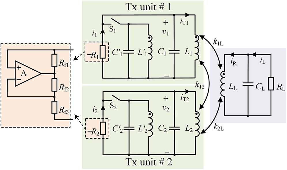
The simplified circuit schematic of the proposed dual-Tx WPT system is shown in Fig. 1, consisting of three resonators with the subscripts “1,” “2,” and “L” for the Tx unit #1, Tx unit #2, and the load, respectively. These parallel LC resonators have the parameters L 1 = L 2 = L 0, L’ 1 = L’ 2 = L’ 0, C 1 = C 2 = C 0, and C’ 1 = C’ 2 = C’ 0. Two operating modes are switched using switches S1 and S2. In Mode I, S1 and S2 are closed, leading to an intrinsic resonant frequency ω’ 1 = ω’ 2 = ω’ 0 = ω L = (L I1C I1)−0.5 = (L LC L)−0.5, where L I1 = L 0||L’ 0 and C I1 = C 0||C’ 0 are total inductance and capacitance of one Tx unit, respectively, with the parallel connection symbol “||.” In Mode II, switches S1 and S2 are opened, leading to an intrinsic resonant frequency ω 1 = ω 2 = ω 0 = (L 0C 0)−0.5 for both Tx units. The coupling coefficients between Tx units and the load are kmn, where m and n (with n ≠ m) can be “1,” “2,” or “L.” Without loss of generality, positive values of kmn are assumed. The dual-Tx units are driven by two independent and identical source units and represented by two negative resistances −R 1 and −R 2. Here, the negative resistance is implemented by utilizing a positive-feedback constructed amplifier. The amplitude of the oscillating voltage is close to the DC power supply voltage. In an oscillation period, the amplifier sometimes operates in its linear region and sometimes in its saturation region, depending upon the voltage magnitude at a certain moment. The nonlinear saturation property enables the equivalent negative resistance and corresponding gain to adjust, maintaining a stable oscillation [Reference Assawaworrarit, Yu and Fan36].
Simplified circuit schematic of the dual-Tx WPT system.

The system can be described using the coupled mode theory (CMT) [Reference Haus and Huang39], leading to lower-order equations compared with the circuit theory. Note, however, that CMT presumes weak coupling and minimal loss. Consequently, CMT trades some accuracy for simplicity and incurs errors relative to the exact circuit theory [Reference Wu, Li, Zeng and Hui40]. The energy mode of resonator m is denoted by am, assuming that it obeys the e jωt rule at the operating frequency ω. The amplitude of am is given by |am| = Vm(Cm/2)0.5, where Vm is the voltage amplitude across the capacitance Cm. The total loss rate at the load end γ L, is given by γ L = γ L0 + γ Lp, where γ L0 = 1/(2R LC L) and γ Lp = 1/(2R LpC L) are the loss rates caused by the parasitic parallel resistance R Lp in the inductance L L and the load R L, respectively. At the Tx end, the gain rate g 1 (g 2) is g 1 = g 10 − γ 1p (g 2 = g 20 − γ 2p) after absorbing the loss rate γ 1p (γ 2p) from the parasitic parallel resistance R 1p (R 2p) in the inductance, respectively. It is worth noting that g 1 and g 2 can be equal to 0 when the Tx units self-oscillate without energy coupling with other resonators. In this situation, g 10 (g 20) balances with γ 1p (γ 2p) i.e., g 10 = γ 1p (g 20 = γ 2p). The coupling rate κmn is κmn = 0.5ω Lkmn.
System behavior in Mode I
The system working in Mode I is a PT-symmetric dimer, which has been studied previously [Reference Assawaworrarit, Yu and Fan36]. Here, we design the system as a scaling PT-symmetric dimer [Reference Chen, Sakhdari, Hajizadegan, Cui, MM, El-Ganainy and Alù41]. The Tx and load resonators possess the same intrinsic resonant frequency (i.e., ω’ 0 = ω L) but proportional circuit parameters, i.e., L I1 = L L/x and C I1 = xC L, where x is a scaling factor. In our design, x is set to 2.
Detailed analysis can refer to [Reference Chen, Sakhdari, Hajizadegan, Cui, MM, El-Ganainy and Alù41]. Below, only the main results are presented for simplicity, even though the series LC resonance discussed in [Reference Chen, Sakhdari, Hajizadegan, Cui, MM, El-Ganainy and Alù41] differs slightly from the parallel LC resonance shown in Fig. 1. Without loss of generality, the situation where Tx #1 is on and Tx #2 is off is analyzed. The eigenfrequency solutions ω I0 at the PT-broken and ω I ± at the PT-symmetric state are given by
 \begin{equation}\left\{ \begin{gathered}
{\omega _{{\text{I0}}}} = {\omega _{\text{L}}}{\text{, when }}{\kappa _{{\text{1L}}}} \lt {\kappa _{\text{c}}} \hfill \\
{\omega _{{\text{I}} \pm }} = {\omega _{\text{L}}} \pm \sqrt {\kappa _{{\text{1L}}}^2 - \gamma _{\text{L}}^2} {\text{, when }}{\kappa _{{\text{1L}}}} \geqslant {\kappa _{\text{c}}} \hfill \\
\end{gathered} \right.,\,\end{equation}
where κ c is the critical coupling rate, κ c = γ L, which distinguishes the PT-symmetric (κ 1L > κ c) from the PT-broken states (κ 1L < κ c). The voltage amplitude ratio can be obtained from the energy mode ratio,
 \begin{equation}\frac{{{V_{\text{L}}}}}{{{V_1}}} = \sqrt {\frac{{{C_{{\text{I}}1}}}}{{{C_{\text{L}}}}}} \frac{{\left| {{a_{\text{L}}}} \right|}}{{\left| {{a_{\text{1}}}} \right|}} = \sqrt x \frac{{\left| {{a_{\text{L}}}} \right|}}{{\left| {{a_{\text{1}}}} \right|}} = \left\{ \begin{gathered}
{{\sqrt x {\kappa _{1{\text{L}}}}} \mathord{\left/
{\vphantom {{\sqrt x {\kappa _{1{\text{L}}}}} {{\gamma _{\text{L}}}}}} \right.
} {{\gamma _{\text{L}}}}}{\text{, when }}{\kappa _{{\text{1L}}}} \lt {\kappa _{\text{c}}} \hfill \\
\sqrt x {\text{, when }}{\kappa _{{\text{1L}}}} \geqslant {\kappa _{\text{c}}} \hfill \\
\end{gathered} \right.,\end{equation}
The voltage amplitude V 1 is approximately 21.5V D/π for a self-oscillating full bridge inverter [Reference Chen, Qiu, Rong and Zhang42] and V S for a positive-feedback constructed amplifier [Reference Assawaworrarit, Yu and Fan36], respectively, where V D is the DC power supply voltage, and V S is the maximum output voltage of the amplifier, which depends on specific amplifiers. Here, the latter will be implemented. As observed from (2), the voltage amplitude V L is scaled x 0.5 times from V 1 (V 1 ≈ V S), i.e., V L = x 0.5V S. The PDL (P IL) and PTE (η I), respectively, are,
 \begin{equation}{P_{{\text{IL}}}} \approx \left\{ \begin{gathered}
{{xV_{\text{S}}^2\kappa _{1{\text{L}}}^2} \mathord{\left/
{\vphantom {{xV_{\text{S}}^2\kappa _{1{\text{L}}}^2} {\left( {2{R_{\text{L}}}\gamma _{\text{L}}^2} \right)}}} \right.
} {\left( {2{R_{\text{L}}}\gamma _{\text{L}}^2} \right)}}{\text{, when }}{\kappa _{{\text{1L}}}} \lt {\kappa _{\text{c}}} \hfill \\
{{xV_{\text{S}}^2} \mathord{\left/
{\vphantom {{xV_{\text{S}}^2} {\left( {2{R_{\text{L}}}} \right)}}} \right.
} {\left( {2{R_{\text{L}}}} \right)}}{\text{, when }}{\kappa _{{\text{1L}}}} \geqslant {\kappa _{\text{c}}} \hfill \\
\end{gathered} \right.\end{equation}
 \begin{equation}{\eta _{\text{I}}} = \left\{ \begin{gathered}
\frac{{{x \mathord{\left/
{\vphantom {x {{R_{\text{L}}}}}} \right.
} {{R_{\text{L}}}}}}}{{x\left( {{1 \mathord{\left/
{\vphantom {1 {{R_{\text{L}}}}}} \right.
} {{R_{\text{L}}}}} + {1 \mathord{\left/
{\vphantom {1 {{R_{{\text{Lp}}}}}}} \right.
} {{R_{{\text{Lp}}}}}}} \right) + {{\gamma _{\text{L}}^2} \mathord{\left/
{\vphantom {{\gamma _{\text{L}}^2} {\kappa _{1{\text{L}}}^2{R_{{\text{1p}}}}}}} \right.
} {\kappa _{1{\text{L}}}^2{R_{{\text{1p}}}}}}}}{\text{, when }}{\kappa _{{\text{1L}}}} \lt {\kappa _{\text{c}}} \hfill \\
\frac{{{x \mathord{\left/
{\vphantom {x {{R_{\text{L}}}}}} \right.
} {{R_{\text{L}}}}}}}{{x\left( {{1 \mathord{\left/
{\vphantom {1 {{R_{\text{L}}}}}} \right.
} {{R_{\text{L}}}}} + {1 \mathord{\left/
{\vphantom {1 {{R_{{\text{Lp}}}}}}} \right.
} {{R_{{\text{Lp}}}}}}} \right) + {1 \mathord{\left/
{\vphantom {1 {{R_{{\text{1p}}}}}}} \right.
} {{R_{{\text{1p}}}}}}}}{\text{, when }}{\kappa _{{\text{1L}}}} \geqslant {\kappa _{\text{c}}} \hfill \\
\end{gathered} \right..\end{equation}
As seen from (2), (3), and (4), a constant amplitude ratio, PDL, and PTE can be achieved if κ 1L ≥ κ c.
System behavior in Mode II
In Mode II, the coupling rates κ 1L ≈ κ 2L should be satisfied. The state equations can be expressed as
 \begin{equation}\left\{ \begin{gathered}
{\text{j}}{{d{a_{1\left( 2 \right)}}} \mathord{\left/
{\vphantom {{d{a_{1\left( 2 \right)}}} {dt}}} \right.
} {dt}} = \left( { - {\omega _0} + {\text{j}}{g_{1\left( 2 \right)}}} \right){a_{1\left( 2 \right)}} - {\kappa _{12}}{a_{2\left( 1 \right)}} - {\kappa _{1{\text{L}}\left( {2{\text{L}}} \right)}}{a_{\text{L}}} \hfill \\
{\text{j}}{{d{a_{\text{L}}}} \mathord{\left/
{\vphantom {{d{a_{\text{L}}}} {dt}}} \right.
} {dt}} = \left( { - {\omega _{\text{L}}} - {\text{j}}{\gamma _{\text{L}}}} \right){a_{\text{L}}} - {\kappa _{{\text{1L}}}}{a_{\text{1}}} - {\kappa _{{\text{2L}}}}{a_{\text{2}}} \hfill \\
\end{gathered} \right..\end{equation}
The condition κ 1L ≈ κ 2L makes the two Tx units behave similarly. Therefore, g 1 ≈ g 2 = g T can be deduced. The two Tx units can be synthesized as an equivalent resonator with an energy mode a T, intrinsic resonant frequency ω T, and gain rate g T. Then the state equations can be described as
 \begin{equation}\left\{ \begin{gathered}
{\text{j}}{{d{a_{\text{T}}}} \mathord{\left/
{\vphantom {{d{a_{\text{T}}}} {dt}}} \right.
} {dt}} = \left( { - {\omega _{\text{T}}} + {\text{j}}{g_{\text{T}}}} \right){a_{\text{T}}} - {\kappa _{{\text{TL}}}}{a_{\text{L}}} \hfill \\
{\text{j}}{{d{a_{\text{L}}}} \mathord{\left/
{\vphantom {{d{a_{\text{L}}}} {dt}}} \right.
} {dt}} = \left( { - {\omega _{\text{L}}} - {\text{j}}{\gamma _{\text{L}}}} \right){a_{\text{L}}} - {\kappa _{{\text{TL}}}}{a_{\text{T}}} \hfill \\
\end{gathered} \right.,\end{equation}
where κ TL is the equivalent coupling rate between the synthesized Tx and the load. Comparing the second rows of (5) and (6), we have κ TLa T = κ 1La 1 + κ 2La 2. Substituting this relation into (6), we have
 \begin{equation}{a_{1\left( 2 \right)}} \approx \frac{{{\kappa _{{\text{1L}}\left( {2{\text{L}}} \right)}}\left( {\omega - {\omega _0} + {\text{j}}{g_{\text{T}}}} \right) + {\kappa _{{\text{12}}}}{\kappa _{{\text{2L}}\left( {1{\text{L}}} \right)}}}}{{{{\left( {\omega - {\omega _0} + {\text{j}}{g_{\text{T}}}} \right)}^2} - \kappa _{12}^2}}{a_{\text{L}}},\end{equation}
where ω − ω 0 + jg T should not be 0. Then, we have
 \begin{equation}{\kappa _{{\text{TL}}}}{a_{\text{T}}} \approx \frac{{\kappa _{1{\text{L}}}^2 + \kappa _{{\text{2L}}}^2}}{{\omega - {\omega _0} - {\kappa _{{\text{12}}}} + {\text{j}}{g_{\text{T}}}}}{a_{\text{L}}}.\end{equation}
At the same time, from the first row of (6), a T can be expressed as κ TLa T = [(κ TL)2/(ω − ω T + jg T)]a L. Comparing this equation with (8), κ TL and ω T can be obtained,
 \begin{equation}\begin{gathered}
{\kappa _{{\text{TL}}}} \approx \sqrt {\kappa _{{\text{1L}}}^2 + \kappa _{{\text{2L}}}^2} \approx \sqrt 2 {\kappa _{1{\text{L}}}}\,. \hfill \\
{\omega _{\text{T}}} = {\omega _{\text{0}}} + {\kappa _{12}} \hfill \\
\end{gathered} \end{equation}
The equivalent intrinsic resonant frequency ω T deviates from ω 0 with an offset κ 12. Then, if we define energy mode vector a = [a T a L]T, a second-order Hamiltonian H of this system can be obtained,
 \begin{equation}{\text{j}}\frac{d}{{dt}}{\mathbf{a}} = {\mathbf{Ha}} = \left[ {\begin{array}{*{20}{c}}
{ - {\omega _{\text{T}}} + {\text{j}}{g_{\text{T}}}}&{ - {\kappa _{{\text{TL}}}}} \\
{ - {\kappa _{{\text{TL}}}}}&{ - {\omega _{\text{L}}} - {\text{j}}{\gamma _{\text{L}}}}
\end{array}} \right]\left[ {\begin{array}{*{20}{c}}
{{a_{\text{T}}}} \\
{{a_{\text{L}}}}
\end{array}} \right]\,.\end{equation}
This Hamiltonian H holds invariant under joint parity-reversal (swapping the subscripts “T” and “L”) and time-reversal (changing the sign of j) operations, if the intrinsic resonant frequency ω L = ω T. Note that in Mode I, ω’ 0 = ω L must be satisfied. Then, to satisfy ω T = ω’ 0 = ω L, based on (9), the frequency ω 0 should be designed as
 \begin{equation}{\omega _0} = {\omega {^{\prime}}_0} - {\kappa _{12}} = {\omega _{\text{L}}} - {\kappa _{12}}.\end{equation}
It should be mentioned that the polarity of the coupling rate κ 12 can be positive or negative, depending upon the polarity of the mutual inductance between the two Tx unit coils.
The frequency solutions can be obtained from det(ω I + H) = 0, where I is the identity matrix,
 \begin{equation}\Delta {\omega ^2} + {g_{\text{T}}}{\gamma _{\text{L}}} - \kappa _{{\text{TL}}}^2 + {\text{j}}\Delta \omega \left( {{g_{\text{T}}} - {\gamma _{\text{L}}}} \right) = 0,\end{equation}
where Δω = ω − ω L. After separating the real and imaginary parts of (11), we have the real eigenvalue solutions
 \begin{equation}\left\{ \begin{gathered}
{\omega _{{\text{II0}}}} = {\omega _{\text{L}}}{\text{, when }}{\kappa _{{\text{TL}}}} \lt {\kappa _{\text{c}}} \hfill \\
{\omega _{{\text{II}} \pm }} = {\omega _{\text{L}}} \pm \sqrt {\kappa _{{\text{TL}}}^2 - \gamma _{\text{L}}^2} {\text{, when }}{\kappa _{{\text{TL}}}} \geqslant {\kappa _{\text{c}}} \hfill \\
\end{gathered} \right..\end{equation}
When κ TL ≥ κ c, the system works at the PT-symmetric state with balanced gain and loss, i.e., g T = γ L. In this region, two real bifurcation frequencies (ω II+ and ω II−) exist. On the other hand, when κ TL < κ c, the system works at the PT-broken state, whose gain should be g T = κ 2TL/γ L.
The ratio |a L|/|a T| can be derived after substituting the frequency solutions into (12). Note that a 1 ≈ a 2 is valid, as derived from (7). Then, κ TLa T = κ 1La 1 + κ 2La 2 ≈ 2κ 1La 1 and a T ≈ 20.5a 1 can be obtained. If the capacitances C 1 and C L are identical, the voltage amplitude ratio is
 \begin{equation}\frac{{{V_{\text{L}}}}}{{{V_1}}} = \sqrt 2 \sqrt {\frac{{{C_1}}}{{{C_{\text{L}}}}}} \frac{{\left| {{a_{\text{L}}}} \right|}}{{\left| {{a_{\text{1}}}} \right|}} = \left\{ \begin{gathered}
{{\sqrt 2 {\kappa _{{\text{TL}}}}} \mathord{\left/
{\vphantom {{\sqrt 2 {\kappa _{{\text{TL}}}}} {{\gamma _{\text{L}}}}}} \right.
} {{\gamma _{\text{L}}}}}{\text{, when }}{\kappa _{{\text{TL}}}} \lt {\kappa _{\text{c}}} \hfill \\
\sqrt 2 {\text{, when }}{\kappa _{{\text{TL}}}} \geqslant {\kappa _{\text{c}}} \hfill \\
\end{gathered} \right..\end{equation}
If the inductances L 1 and L L are designed as identical, the capacitances C 1 and C L should satisfy C L = (1 − 0.5k 12)2C 1, based on (11). Because the two Tx units can be placed closely together, the coupling coefficient k 12 and these capacitances can be considered as fixed values. In Mode II, V 1 is still approximately equal to V S. Then, we can find the PDL P IIL = 2γ L0|a L|2 can be expressed as
 \begin{equation}{P_{{\text{IIL}}}} \approx \left\{ \begin{gathered}
{{V_{\text{S}}^2\kappa _{{\text{TL}}}^2} \mathord{\left/
{\vphantom {{V_{\text{S}}^2\kappa _{{\text{TL}}}^2} {\left( {{R_{\text{L}}}\gamma _{\text{L}}^2} \right)}}} \right.
} {\left( {{R_{\text{L}}}\gamma _{\text{L}}^2} \right)}}{\text{, when }}{\kappa _{{\text{TL}}}} \lt {\kappa _{\text{c}}} \hfill \\
{{V_{\text{S}}^2} \mathord{\left/
{\vphantom {{V_{\text{S}}^2} {{R_{\text{L}}}}}} \right.
} {{R_{\text{L}}}}}{\text{, when }}{\kappa _{{\text{TL}}}} \geqslant {\kappa _{\text{c}}} \hfill \\
\end{gathered} \right..\end{equation}
As observed from (15), when κ TL ≥ κ c, the PDL P IIL is not only insensitive to the coupling coefficient, but also can be the same as the PDL in Mode I, if the scaling factor x is set to 2.
From (15), the PTE η II can be obtained,
 \begin{equation}{\eta _{{\text{II}}}} = \left\{ \begin{gathered}
\frac{{{1 \mathord{\left/
{\vphantom {1 {{R_{\text{L}}}}}} \right.
} {{R_{\text{L}}}}}}}{{{1 \mathord{\left/
{\vphantom {1 {{R_{\text{L}}}}}} \right.
} {{R_{\text{L}}}}} + {1 \mathord{\left/
{\vphantom {1 {{R_{{\text{Lp}}}}}}} \right.
} {{R_{{\text{Lp}}}}}} + {{\gamma _{\text{L}}^2} \mathord{\left/
{\vphantom {{\gamma _{\text{L}}^2} {\kappa _{1{\text{L}}}^2{R_{{\text{1p}}}}}}} \right.
} {\kappa _{1{\text{L}}}^2{R_{{\text{1p}}}}}}}}{\text{, when }}{\kappa _{{\text{1L}}}} \lt {\kappa _{\text{c}}} \hfill \\
\frac{{{1 \mathord{\left/
{\vphantom {1 {{R_{\text{L}}}}}} \right.
} {{R_{\text{L}}}}}}}{{{1 \mathord{\left/
{\vphantom {1 {{R_{\text{L}}}}}} \right.
} {{R_{\text{L}}}}} + {1 \mathord{\left/
{\vphantom {1 {{R_{{\text{Lp}}}}}}} \right.
} {{R_{{\text{Lp}}}}}} + {1 \mathord{\left/
{\vphantom {1 {{R_{{\text{1p}}}}}}} \right.
} {{R_{{\text{1p}}}}}}}}{\text{, when }}{\kappa _{{\text{1L}}}} \geqslant {\kappa _{\text{c}}} \hfill \\
\end{gathered} \right..\end{equation}
We can find that the operating Mode II has the same behaviors as the operating Mode I, except for their different coupling coefficient expressions. That is because the energy modes a 1 and a 2 are synthesized into an equivalent energy mode a T due to their synchronization in phase, as seen from (7). Moreover, the amplitudes of a 1 and a 2 are close to each other when κ 1L ≈ κ 2L. It indicates that the coupling between the two Tx units merely guides the two resonators to oscillate in phase, with almost no energy exchange between them.
Interestingly, in Mode II, besides the in-phase working state of the two Tx units, a potential out-of-phase working state also exists. The frequency solution ω II4 = ω 0 and corresponding g 1 = g 2 = 0, as derived from (5), results in ω − ω 0 + jg 1 = ω − ω 0 + jg 2 = 0. From (5), we also find that a L = 0 and κ 1La 1 = −κ 2La 2. Based on the previous assumption of positive coupling coefficients, a 1 and a 2 are out of phase. The energies from the two Tx units on the load cancel each other out. The two Tx units appear to be self-oscillating independently. Therefore, it is necessary to develop methods that will enable the system to operate at the in-phase state.
Phase synchronization of two coupled resonators
The synchronization of coupled oscillators can be traced back to Huygens’ study of a pair of adjacent pendulum clocks mounted on the same vertical support in 1665 [Reference Jenkins43]. The synchronization of relaxation oscillators is extensively studied across various fields such as mechanics, electronics, biology, and sociology. For instance, it explains how thousands of fireflies can flash synchronously [Reference Mirollo and Strogatz44]. The Tx units in our system are examples of Van der Pol oscillators [Reference van der Pol45]. The dynamics of two magnetically coupled Van der Pol oscillators were studied in [Reference Kana, Fomethe, Fotsin and Fotso46–Reference Tegnitsap and Fotsin48]. As stated in these studies, if the coupling between the two oscillators is strong enough, they tend to form phase synchronization. Inspired by these studies, we can synchronize the two Tx units in our system in phase if they are coupled directly without the load end. The natural coupling between them can be enhanced by placing the two Tx coils closer to each other. Note that this mutual coupling is not desirable in traditional multiple Tx systems. When the two synchronous oscillators are loaded through inductive couplings, the in-phase oscillation will continue, similar to inertia.
The dynamics of coupled oscillators are typically analyzed using time-domain state equations, because observing possible chaotic phenomena is difficult in the frequency domain. The time-domain state equations of the circuit, as shown in Fig. 1, without the load end, are given by
 \begin{equation}\left\{ \begin{gathered}
{C_0}{{d{v_m}} \mathord{\left/
{\vphantom {{d{v_m}} {dt}}} \right.
} {dt}} = {i_m} - {i_{{\text{T}}m}} \hfill \\
{v_m} = {L_0}{{d{i_{{\text{T}}m}}} \mathord{\left/
{\vphantom {{d{i_{{\text{T}}m}}} {dt}}} \right.
} {dt}} - {k_{12}}{L_0}{{d{i_{{\text{T}}n}}} \mathord{\left/
{\vphantom {{d{i_{{\text{T}}n}}} {dt}}} \right.
} {dt}} \hfill \\
{i_m} = a{v_m} - bv_m^3 \hfill \\
\end{gathered} \right.,\,\,\,\,\,\,\,\,\,\,\,\,\,\,\end{equation}
where m and n (with n ≠ m) are 1 or 2, im is the instantaneous output current of the negative resistance – Rm, i Tm is the instantaneous current of the Tx inductance Lm, and vm is the instantaneous voltage on the capacitance Cm, as shown in Fig. 1. The current-voltage characteristic of the negative resistance – Rm is modeled with a cubic function im = avm − b(vm)3, where a > 0 and b > 0 are two positive coefficients whose specific values depend upon specific circuit parameters [Reference Kana, Fomethe, Fotsin and Fotso46–Reference Shinriki, Yamamoto and Mori50]. The state equation can be arranged as first-order ordinary differential equations (ODEs),
 \begin{equation}\left\{ \begin{gathered}
\frac{d}{{dt}}{v_m} = \frac{a}{{{C_0}}}{v_m} - \frac{b}{{{C_0}}}v_m^3 - \frac{1}{{{C_0}}}{i_{{\text{T}}m}} \hfill \\
\frac{d}{{dt}}{i_{{\text{T}}m}} = \frac{{{k_{12}}}}{{\left( {1 - k_{12}^2} \right){L_0}}}{v_n} + \frac{1}{{\left( {1 - k_{12}^2} \right){L_0}}}{v_m} \hfill \\
\end{gathered} \right..\end{equation}
The ODEs in (18) can be solved using the Runge–Kutta methods available within the ode45-solver in Matlab (R2021b, MathWorks). Figure 2 shows the error |i T1 − i T2| between the currents i 1 and i 2 as a function of the coupling coefficient k 12. The parameters are consistent with those of the experimental prototype, in which the inductance L 0 is 10.9 μH and the capacitance C 0 is 265 pF, respectively. The resistances R f1 = 51 Ω, R f2 = 470 Ω, and R f3 = 4.7 kΩ around the operational amplifier are utilized to form a minimum achievable negative resistance − R f1R f3/R f2 = −510 Ω. The nonlinear saturation characteristic of the operational amplifier allows the effective negative resistance to adjust adaptively in response to the voltage amplitude of the oscillation. That is, as the voltage increases, the negative resistance will gradually increase, eventually becoming zero and even a positive resistance. Here, the current-voltage function is im = 2.06 × 10⁻³vm − 2.66 × 10⁻⁶(vm)3. The initial condition for the results shown in Fig. 2, as an example, is (v 1, i 1) = (2 mV, 0.5 mA) and (v 2, i 2) = (1 mV, 0.3 mA).
Calculated |i T1 − i T2| as a function of the coupling coefficient k 12.

As observed from Fig. 2, the error |i 1 − i 2| varies over time when the two oscillators exhibit chaotic behavior, a condition that occurs when k 12 is below the threshold of approximately 0.05. When k 12 is higher than the threshold, the two oscillations are in phase and have the same magnitude, resulting in |i 1 − i 2| = 0. In our design, the two square-shaped Tx coils are positioned in close proximity to each other to achieve a sufficiently strong coupling.
Comparison with other PT-symmetric WPTs
The two operating modes of the proposed system are compared with those of other PT-symmetric WPT systems, as presented in Table 1. In Mode I, the system is designed as the scaling PT-symmetric dimer [Reference Chen, Sakhdari, Hajizadegan, Cui, MM, El-Ganainy and Alù41], which employs a single source and single coil (SSSC) structure at the Tx. Note that only one Tx unit is activated in Mode I. Recently, in order to address the misalignment issue between the Tx and Rx coils, the structure with single source and dual coils (SSDC) is proposed in [Reference Chen, Qiu, Rong and Zhang42], where dual Tx coils are connected in parallel with wired connections and driven by a single self-oscillating power source. Because the two parallel-connected coils form a single coil, the SSDC structure actually is the same as the SSSC structure. In Mode II of our proposed system, the system forms a structure with dual sources and dual coils (DSDC), in which two independent Tx coils are utilized. The two independent Tx coils can be equivalent to a single coil when the two Tx units work at the in-phase state. The equivalent effective coupling coefficients in Table 1 for the SSDC and DSDC structures are obtained by synthesizing the two Tx coils into one equivalent Tx coil. Note that, in [Reference Chen, Qiu, Rong and Zhang42], the equivalent effective coupling for the SSDC structure is defined as k and k = (k 1Lk 2L)0.5. Therefore, for the SSDC structure, the relation between k TL (denoted as k TL,SSDC) and k is k TL,SSDC = 20.5k.
Comparison of the proposed system with traditional single-source driven PT-symmetric WPTs

Comparing the three structures in Table 1, first, the equivalent effective coupling coefficient k TL of the DSDC structure is always larger than that of the SSDC structure, because (k 1L)2 +(k 2L)2 ≥ 2k 1Lk 2L is valid. When k 1L = k 2L and (k 1L)2 +(k 2L)2 = 2k 1Lk 2L, the two Tx units in the DSDC structure are totally the same as the wired-connected SSDC structure. The k TL of the DSDC structure is also always larger than that of the SSSC structure (i.e., k 1L). However, for the k TL of the SSDC structure to be larger than that of the SSSC structure, k 2L must be larger than 0.5k 1L, which depends upon the relative position between the Tx and Rx coils. The proposed DSDC structure features the highest k TL and extends the power transfer region with robust PDL.
Second, the critical coupling coefficient of k 1L when k 1L = k 2L is reduced for the SSDC and DSDC structures compared to the SSSC structure. For the SSSC structure, the critical coupling coefficient of k 1L approximates to 1/Q L, where Q L is the quality factor of the load circuit and Q L = 0.5ω L/γ L. While for the SSDC and DSDC structures, the critical coupling coefficient of k 1L is reduced to 1/(20.5Q L), with a 1/20.5 scaling factor compared to the SSSC structure. About 12.5% critical coupling coefficient of k 1L (which is equal to k when k 1L = k 2L) is reduced in experiments as reported in [Reference Chen, Qiu, Rong and Zhang42]. This reduction indicates a longer transfer distance or a larger lateral transfer region for invariant PDL.
Third, with the same power supply voltage, identical PDL can be achieved in these three structures if the scaling factor x is set to 2 in the SSSC structure. That also means a robust PDL can be implemented by switching between Mode I and Mode II in the proposed DSDC structure. The PTEs of the structures with two Tx coils, SSDC and DSDC, are the same but slightly smaller than those of the SSSC structure when x = 2.
Fourth, although the DSDC structure is similar to the SSDC structure, it offers the advantage of flexible assembly and an extended lateral wireless charging region. As stated previously, the SSDC structure is actually a special case of the SSSC structure, achieved by separating a single coil into two wire-connected coils. In our design, the DSDC structure is implemented by combining two SSSC structures through wireless coupling. The side-by-side placement of two independent Tx coils, as presented in the next section, effectively extends the lateral wireless charging region, compared to the single Tx coil structure.
Experimental verification
The experimental setup is shown in Fig. 3(a). All the coils are identical and printed on PCBs (printed circuit boards). The enlarged view of the Tx coils is shown in Fig. 3(b). The outer side length of each Tx coil is 3.6 cm, which is close to the size of the wireless charging platform for mobile phones. Two independent Tx coils, when placed side by side, can extend the lateral wireless charging region and offer flexibility in assembly. The inductances L’ 1 and L’ 2 in our proposed system can be implemented using compact lumped inductors. For simplicity, in our experimental setup, they are implemented with PCB spiral coils, as shown in Fig. 3(b), using the same structure as L 1 and L 2, and are placed far away from the Rx coil.
(a) Experimental setup. (b) Enlarged view of Tx coils.

The electrical parameters, including the inductances, capacitances, parasitic parallel resistances, and resonant frequencies, are listed in Table 2. These parameters are measured using an impedance analyzer (E4990A, Keysight). In Mode I, the switch S1 is closed, and the two inductances L 1 and L’ 1 are connected in parallel. The measured intrinsic resonant frequencies of both the Rx resonator (i.e., f L = ω L/2π) and the Tx resonator in Mode I (i.e., f’ 0 = ω’ 0/2π) are about 2.86 MHz. In Mode II, the switches S1 and S2 are open. The intrinsic resonant frequency of each independent Tx resonator unit (i.e., f 0 = ω 0/2π) is measured to be 2.96 MHz. When placing the two Tx coils side by side, as shown in Fig. 3(b), the resonant frequency is reduced to 2.86 MHz due to the coupling coefficient k 12. Note that the polarity of k 12 is negative in our experiments. Therefore, the frequency relation as shown in (11) is satisfied.
Electrical parameters of the system

The simulated and measured voltages v 1 and v 2 across the capacitances C 1 and C 2, respectively, are illustrated in Fig. 4(a) and 4(b) using PSPICE and through an oscilloscope (MDO34, Tektronix). The PSPICE simulation circuit schematic corresponds to Fig. 1, and all electrical parameters are listed in Table 2. The resistors connected to the operational amplifier (LM7171A, TI) are R f1 = 51 Ω, R f2 = 470 Ω, and R f3 = 4.7 kΩ. In Fig. 4(b), to clearly distinguish the two voltages, different vertical scales (5 and 2 V/div) are set for them. The simulated and measured results indicate that the two voltages oscillate in phase with a coupling coefficient k 12 of 0.074, which is larger than the theoretically predicted threshold value 0.05, as shown in Fig. 2.
(a) Simulated and (b) measured voltages v 1 and v 2 across the capacitances C 1 and C 2, respectively.

The system performance is validated through moving the Rx coil along the X direction, as shown in Fig. 3(a). The center of the Rx coil is moved within the range −4 cm < X < 4 cm, with the vertical distance Z fixed at 0.5 cm. The absolute values of the coupling coefficients between the Rx coil and the Tx coils are measured and presented in Fig. 5. In Fig. 5, the red line represents the coupling coefficient k 1L in Mode I between the Rx inductance L L and the Tx inductance, which consists of the parallel-connected inductances, i.e., L 1||L’ 1. Correspondingly, the black line represents k 2L between the inductances L L and L 2||L’ 2. The equivalent effective coupling coefficient k TL in Mode II, as shown by the blue line in Fig. 5, is obtained from the measured k 1L and k 2L in accordance with (9), k TL = [(k 1L)2 +(k 2L)2]0.5. As a comparison, Fig. 5 also shows the coupling coefficient of the SSDC structure k TL,SSDC = (2k 1Lk 2L)0.5. Note that the coupling coefficient of the SSSC structure is the same as the value in Mode I of the DSDC structure. As observed from Fig. 5, k TL is significantly larger than k TL,SSDC, for almost all positions of the Rx coil except when the Rx coil is located at the center of the two Tx coils, where k 1L ≈ k 2L.
Measured coupling coefficients of the DSDC and SSDC structure as a function of X directional distance. The values in Mode I of the DSDC structure are the same as those of the SSDC structure.

Figure 6(a) shows the operating frequency f (f = ω/2π) as the Rx coil is moved along the X direction. The calculated frequency is consistent with both the simulated and measured frequencies. Although two possible calculated eigenfrequencies exist at the PT-symmetric state, as predicted in (1) and (13), only one frequency is selected as the operating frequency in practice due to the bistable characteristic [Reference Assawaworrarit, Yu and Fan36].
Comparison of calculated, simulated, and measured (a) operating frequency, (b) voltage amplitude ratio V L/V 1, (c) PDL, and (d) PTE.

The selection of either the high-frequency or low-frequency branch depends on the initial conditions of the specific self-oscillation circuits. The PT-broken and PT-symmetric regions are distinguished by a critical coupling coefficient k c. The calculated k c is k c = ω LL L/(R L||R Lp) ≈ 0.140, which agrees with the simulated and measured results, as shown in Fig. 6(a). The measured k c is 0.144, which corresponds to both k 1L and k 2L being about 0.100 when k 1L = k 2L in the SSDC structure and the Mode II of the DSDC structure. In Mode I, if only Tx unit #1 is active, the measured critical coupling coefficient for k 1L is 0.144.
Based on the measured coupling coefficients in Fig. 5, if Mode I operation is selected, the system works at the PT-symmetric state when the center of the Rx coil is located within the range of 0.2 cm ≤ |X| ≤ 3.4 cm and either k 1L or k 2L is larger than k c. When |X| < 0.2 cm, Mode II should be selected as the operating mode, whose equivalent effective coupling coefficient k TL is larger than k c. Although k TL in Mode II is larger than k c within the range 0.2 cm ≤ |X| ≤ 3.4 cm, in this region, the system is inefficient. That is because there is a significant difference between k 1L and k 2L, due to the high sensitivity of the coupling coefficients to the lateral misalignment of the coil. Without loss of generality, assuming that X > 0.2 cm, the ratio k 1L/k 2L > 2 can be observed in Fig. 5. In this situation, from the efficiency perspective, the Tx unit #2 should be deactivated, with only Tx unit #1 remaining active. That is, Mode I should be activated in this situation.
Figure 6(b)–6(d) illustrates the performances of the voltage amplitude ratio V L/V 1, PDL, and PTE, respectively, both for the traditional SSSC structure and the proposed structure. Due to the symmetry of the Tx units #1 and #2, in the traditional SSSC structure, only the performance using the Tx unit #1 is shown here. For the proposed structure, the two operating modes are indicated by different background colors in the figures. It can be observed that the calculated results of V L/V 1, PTE, and PDL are in good agreement with the simulated and measured results, respectively.
As seen in Fig. 6(b), for the proposed structure, the measured V L/V 1 is stable at around 1.29 in Mode I and 1.27 in Mode II, which are slightly lower than the calculated values of 1.41. In fact, the CMT used in the calculation simplifies the analysis but sacrifices accuracy and introduces some errors, compared with the exact circuit theory [Reference Wu, Li, Zeng and Hui40]. Thus, even in the same operating mode, as the operating frequency varies, the voltage amplitude ratio is not constant in practice. At the same time, due to the uncertainty and mismatch of the electronic components in practice, the capacitance C 1 and C’ 1 in parallel are not exactly equal to 2C 1, which in turn causes the ratios of V L/V 1 in the two operating modes to be not exactly equal as well. In addition, the coupling coefficient k 12 causes a discrepancy between the energy modes of the two Tx units in Mode II, as presented in (7). Although the ratio V L/V 1 is not ideally constant, it is relatively stable even within the X-distance region of Mode II, where it will decrease to as low as 0.8 in the case of the SSSC structure.
The PDL, as shown in Fig. 6(c), has the same behavior as the voltage ratio V L/V 1. Because the amplitude V 1 is almost invariant and approximates the maximum output voltage V S (≈8 V) of the amplifier, the PDL in the entire Rx moving region where |X| ≤ 3.4 cm is about 40 mW, remaining robust thanks to the two operating modes in the proposed structure. The required power level depends on specific applications. The 40-mW level PDL can be used for low-power consumer electronics. A higher PDL can be achieved by optimizing both the coupling parameters and the power capability of the source. For example, for an application whose equivalent load resistance is lower than the present 1.6 kΩ, while leaving the coupling structures unchanged (coil inductances and coupling coefficients), larger capacitances can be employed to lower the resonant frequency while maintaining the load-circuit quality factor Q L. At the Tx end, the power capability can be increased either by raising the DC supply voltage or by adopting more efficient self-oscillating power sources, such as full-bridge inverters [Reference Chen, Qiu, Rong and Zhang42, Reference Assawaworrarit and Fan51]. In addition, the PCB coils may be replaced by Litz-wired coils with a larger cross-sectional area, higher current capacity, and lower power dissipation.
As depicted in Fig. 6(d), the measured and simulated PTEs within the working region are about 72%, which are close to the calculated values, and remain unchanged relative to the lateral movement of the Rx. The power loss is primarily due to the parasitic resistances of the coils. The PCB coil in this work has a lower quality factor (about 47) than the Litz wire, due to the lower thickness (∼35 μm) in PCB coils, which introduces more resistive loss because of the skin-effect and proximity-effect of alternating current crowding phenomenon [Reference Feng, Yeon, Cheng, Ghovanloo and Constandinou52–Reference Jow and Ghovanloo54]. The PTE is larger than 90% as demonstrated in [Reference Chen, Qiu, Rong and Zhang42], where Litz wires with quality factors of about 369 are used. The lower quality factor indicates a larger power loss and lower PTE. However, PCB coils offer the advantage of standard manufacturing processes.
In summary, the proposed system provides stable voltage amplitude ratio V L/V 1, PDL, and PTE over an extended range of lateral power transfer distances. Compared to the SSSC structure, the DSDC structure almost doubles the lateral power transfer range by combining Mode I and Mode II. The proposed system in Mode II can address the performance valley region that exists between the two side-by-side traditional SSSC structures, due to the rapid decrease of the coupling coefficient in this region. In Mode II, the coupling between the two Tx units merely guides the two resonators to oscillate in phase, with almost no energy exchange between them, and without reducing the performance (V L/V 1, PDL, and PTE). Note that the SSDC structure in [Reference Chen, Qiu, Rong and Zhang42] needs to overlap almost completely to maintain a sufficient coupling coefficient, resulting in only a slight extension of the lateral power transfer range. In [Reference Chen, Qiu, Rong and Zhang42], the equivalent diameter is extended by only 20% (from the 35-cm diameter of the single coil to the 42-cm diameter of the two overlapping coils). In addition, the independent Tx units offer the advantage of flexible assembly. This means that in specific applications, one can choose to use either one or two Tx units. The two Tx units can self-organize without the need for a wired connection.
In the future, when two Tx units are utilized, the automatic recognition methods of the required operating modes can be developed, e.g., distinguishing the voltage amplitudes between Mode I and Mode II at the Tx. Additionally, scenarios involving multiple Tx units can be further studied to facilitate the implementation of a large-scale free-positioning wireless charging area in the future.
Conclusion
In this paper, we propose a self-organized PT-symmetric WPT system consisting of dual independent identical Tx units, which offers the advantage of flexible assembly and extension of the lateral power transfer range, compared to traditional SSDC systems. It provides two operating modes employing either one Tx unit or two Tx units, i.e., Mode I and Mode II, respectively. When the proposed system operates in Mode I, it resembles the traditional SSSC structure. In Mode II, with the help of the existing mutual coupling between the two side-by-side Tx units, the two independent Tx units oscillate in phase and address the performance valley region that exists in the middle of the two regions of the operating Mode I. By strategically using a scaled PT-symmetric structure in Mode I with a scaling factor of 2, the voltage on the load equals the value in Mode II. Thus, the system achieves stable output voltage, PDL, and PTE across the entire lateral power transfer distance range, which is extended through the combination of the two operating modes. The behavior of the proposed system is analytically analyzed. The simulated and experimental results validate the theoretical basis and the performance improvement, as compared to the traditional PT-symmetric SSSC and SSDC systems.
Acknowledgments
This work was supported by the “Pioneer” and “Leading Goose” Research and Development Program of Zhejiang and the National Natural Science Foundation of China under Grant Nos. 62141409 and 61771175.
Competing interests
The authors declare no competing interests.