










1 Introduction
In this paper we will be interested in the basic problem of multiplicative Diophantine approximation regarding existence of small values for products
 $$ \begin{align*}q\cdot \|qx_1\| \cdot \|qx_2\|, \quad\text{with } q\in\mathbb{N}, \end{align*} $$
for Lebesgue generic
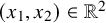
 $\underline {x}=(x_1,x_2)\in \mathbb {R}^2$
, where
 $\|\cdot \|$
denotes the distance to the closest integer. The main result in this direction was established by Gallagher [Reference Gallagher8], who showed that for any nonincreasing function
 $\psi :\mathbb {N}\to \mathbb {R}_+$
satisfying
 $\sum _{q=1}^\infty \psi (q)\frac {\log q}{q}=\infty $
, the inequality
 $$ \begin{align*}q\cdot\|qx_1\|\cdot \|qx_2\|\le\psi(q) \end{align*} $$
has infinitely many solutions
 $q\in \mathbb {N}$
for almost all
 $\underline {x}=(x_1,x_2)\in \mathbb {R}^2$
. For instance, for almost all
 $\underline {x}=(x_1,x_2)\in \mathbb {R}^2$
, there are infinitely many solutions
 $q\in \mathbb {N}$
to the inequality
 $$ \begin{align*}q\cdot\|qx_1\|\cdot \|qx_2\|\le (\log q)^{-2}. \end{align*} $$
The next natural question involves the distribution of the set of solutions
 $$\begin{align*}M(\underline{x}) := \big\{ q \in \mathbb{N} \, : \, q\cdot \|qx_1\| \cdot \|qx_2\|\le \psi(q)\big\}. \end{align*}$$
Wang and Yu [Reference Wang and Yu21] derived an explicit asymptotic formula for the cardinality
 $|M(\underline {x}) \cap [1,T)|$
as
 $T\to \infty $
. Inhomogeneous versions of these problems were also studied by Chow and Technau [Reference Chow and Technau4, Reference Chow and Technau5]. The above results are usually described as asymptotic Diophantine problems.
Here we explore the analogous uniform Diophantine problem that involves solutions to the inequalities
 $$ \begin{align*} q\cdot \|qx_1\| \cdot \|qx_2\|\le b,\quad 1\le q< T \end{align*} $$
for given parameters b and T. It should be noted that there is an essential difference between asymptotic problems and uniform problems. For instance, establishing a uniform version of the classical Khinchin theorem was addressed only recently in [Reference Kleinbock and Wadleigh15, Reference Kleinbock and Rao12, Reference Kleinbock and Rao13]. A somewhat different related uniform problem was also considered by Widmer [Reference Widmer22]. His result concerns the sets
 $$\begin{align*}N(\underline{x};b) := \left\{ q \in \mathbb{N} \, : \, \|qx_1\| \cdot \|qx_2\| \leq b \right\}, \end{align*}$$
and it follows from [Reference Widmer22] that if
 $b\gg (\log T)^{4+\varepsilon }/T$
for some
 $\varepsilon>0$
, then for almost all
 $\underline {x}\in \mathbb {R}^2$
,
 $$ \begin{align*}\big|N(\underline{x};b) \cap [1,T)\big|=4\cdot b(1-\log(4b))\cdot T+O_{\underline{x},\varepsilon}\Big( b^{2/3}(-\log b) \cdot T^{2/3} (\log T)^{4/3+\varepsilon/3} \Big). \end{align*} $$
The condition on the parameter b is probably not optimal and is needed to ensure that the required Diophantine condition in [Reference Widmer22] holds for almost all
 $\underline {x}\in \mathbb {R}^2$
. However, it is not clear whether this method can give an asymptotic formula in a larger range.
Our first main result gives an asymptotic formula for the growth of the sets
 $$\begin{align*}L(\underline{x};b) := \big\{ q \in \mathbb{N} \, : \, q\cdot \|qx_1\| \cdot \|qx_2\|\le b \big\}. \end{align*}$$
Theorem 1.1. Let
 $\eta \in (1,2)$
. Then for every
 $\varepsilon> 0$
and for almost every
 $\underline {x} \in \mathbb {R}^2$
,
-
○ when
 $(\ln T)^{-\eta }\le b\le (\ln T)^{-\eta /(3-\eta )}$
,
$$ \begin{align*} \big|L(\underline{x};b) \cap [1,T)\big| = 2 \cdot b \cdot (\ln T)^2 +O_{\underline{x},\varepsilon}\left( b^{1-1/\eta} \cdot (\ln \ln T)^{6+\varepsilon} \ln T \right), \end{align*} $$
-
○ when
$b\ge (\ln T)^{-\eta /(3-\eta )}$
,
$$ \begin{align*} \big|L(\underline{x};b) \cap [1,T)\big| = 2 \cdot b \cdot (\ln T)^2 +O_{\underline{x},\varepsilon}\left( b^{2/\eta}\cdot (\ln \ln T)^{6+\varepsilon} (\ln T)^2 \right). \end{align*} $$




Theorem 1.1 is proved in Section 11. It will be deduced from a more general result which we now describe.
Given parameters
 $T\ge 1$
and
 $a,b,c>0$
satisfying
 $$\begin{align*}a < b <1 \quad \text{and} \quad c < \frac{1}{2}, \end{align*}$$
we consider the domains
 $$ \begin{align} \Omega=\Omega_{[1,T)}^{(a,b],c} := \left\{ (\underline{u},y) \in \mathbb{R}^2 \times [1,T) \, : \, \begin{array}{c} \max(|u_1|,|u_2|) \leq c \\[0.2cm] a < |u_1u_2| \cdot y \leq b \end{array} \right\}, \end{align} $$
and, for
 $\underline {x} = (x_1,x_2) \in \mathbb {R}^2$
, the corresponding sets
 $$\begin{align*}Q_\Omega(\underline{x}) := \left\{ q \in [1,T) \cap \mathbb{N} \, : \, \begin{array}{c} \max(\|qx_1\|,\|qx_2\|) \leq c \\[0.2cm] a < q\cdot \|qx_1\|\cdot \|qx_2\| \leq b \end{array} \right\}. \end{align*}$$
It is natural to expect that the cardinality
 $|Q_\Omega (\underline {x})|$
grows as the volume of
 $\Omega $
. Our next theorem proves such an asymptotic formula:
Theorem 1.2. Suppose that
 $$\begin{align*}a \ge (\ln T)^{-\theta}\quad \text{and} \quad \zeta\cdot b \le c^2 \quad\text{for some } \zeta,\theta>0. \end{align*}$$
Let
 $\eta \in (1,2)$
. Then for every
 $\varepsilon> 0$
and for almost every
 $\underline {x} \in \mathbb {R}^2$
,
-
○ when
$(c\cdot \ln T)^{-\eta }\le b\le (c\cdot \ln T)^{-\eta /(3-\eta )}$
,
$$ \begin{align*} \big|Q_\Omega(\underline{x})\big| = \operatorname{\mathrm{Vol}}_3(\Omega) +O_{\underline{x},\zeta,\theta,\varepsilon}\left( c^{-1}b^{1-1/\eta} \cdot (\ln \ln T)^{6+\varepsilon} \ln T+1 \right), \end{align*} $$
-
○ when
$b\ge (c\cdot \ln T)^{-\eta /(3-\eta )}$
,
$$ \begin{align*} \big|Q_\Omega(\underline{x})\big| = \operatorname{\mathrm{Vol}}_3(\Omega) +O_{\underline{x},\zeta,\theta,\varepsilon}\left( b^{2/\eta}\cdot (\ln \ln T)^{6+\varepsilon} (\ln T)^2 +1 \right). \end{align*} $$




To compare the above main term with the error term, we note that according to (A.4) in Appendix A,
 $$ \begin{align} \operatorname{\mathrm{Vol}}_3(\Omega) \sim 2 \cdot (\ln T)^2 \cdot (b - a)\quad \text{as } T\to\infty. \end{align} $$
Due to the assumption on the parameter a, we cannot directly take
 $a = 0$
in the Theorem 1.2 to deduce almost sure asymptotics for the sets
 $L(\underline {x};b)$
in Theorem 1.1. Instead we analyze the existence of lattice points in thin hyperbolic strips and show that when a decays sufficiently fast, the sets
 $L(\underline {x},a)$
are empty for almost all
 $\underline {x}\in \mathbb {R}^2$
(see Section 11).
Our method also allows us to study the distribution of the scaled set
 $Q_\Omega (\underline {x})/T$
in the interval
 $[0,1]$
. For a compactly supported Lipschitz function
 $h : \mathbb {R} \rightarrow \mathbb {R}$
consider the weighted counting function
 $$\begin{align*}S_\Omega h(\underline{x}) := \sum_{q \in Q_\Omega(\underline{x})} h\left(\frac{q}{T}\right), \quad \underline{x} \in \mathbb{R}^2. \end{align*}$$
We shall show that
 $S_\Omega h(\underline {x})$
is asymptotic on average to the weighted mean
 $$ \begin{align} \mathcal{M}_\Omega (h) := \int_{1}^T h\left(\frac{y}{T}\right) \cdot \operatorname{\mathrm{Vol}}_2(\Omega(y)) \, dy, \end{align} $$
where
 $$ \begin{align*}\Omega(y) := \{ x \in \mathbb{R}^2 \, : \, (x,y) \in \Omega\}. \end{align*} $$
We note that
 $\operatorname {\mathrm {Vol}}_2(\Omega (y))$
can be computed explicitly (see Lemma A.1). When
 $h = 1$
on the interval
 $[0,1]$
, the sum
 $S_\Omega h(\underline {x})$
is simply
 $|Q_\Omega (\underline {x})|$
and
 $\mathcal {M}_\Omega (h) = \operatorname {\mathrm {Vol}}_3(\Omega )$
. For different oscillatory functions h, the asymptotics of
 $S_\Omega h(\underline {x})$
describe the distribution of
 $Q_\Omega (\underline {x})$
inside
 $[1,T)$
.
We establish a bound for ‘subquadratic’ moments defined in terms of the function
 $$ \begin{align} \theta_\kappa(s):=s^2/\ln(e+|s|)^{1+\kappa}\quad\text{with } \kappa>0. \end{align} $$
Theorem 1.3. With the assumption as in Theorem 1.2, for every compactly supported Lipschitz function
 $h : \mathbb {R} \rightarrow \mathbb {R}$
and
 $\kappa> 0$
,
 $$\begin{align*}\int_{[0,1)^2} \theta_\kappa\Big( S_\Omega h(\underline{x})-\mathcal{M}_\Omega(h) \Big)\, d\underline{x}\ll_{h,\zeta, \theta,\kappa} c^{-2}b\cdot (\ln\ln T)^{3+\kappa} (\ln T)^2. \end{align*}$$
In particular,
 $$\begin{align*}\int_{[0,1)^2} \theta_\kappa\Big( |Q_\Omega(\underline{x})|-\operatorname{\mathrm{Vol}}_3(\Omega) \Big)\, d\underline{x}\ll_{\zeta, \theta,\kappa} c^{-2}b\cdot (\ln\ln T)^{3+\kappa} (\ln T)^2. \end{align*}$$
Remark 1.4. In view of the volume asymptotics (1.2), for certain ranges of the parameters, the formula in Theorem 1.2 establishes an error term with essentially ‘square-root cancellation’.
Theorem 1.3 is proved in Section 9. Then Theorem 1.2 is deduced from it in Section 10 using a Borel-Cantelli argument. We outline the structure of the paper in Section 2 below.
2 Organisation of the paper
It will be convenient to consider a more geometric framework. For
 $\underline {x} \in \mathbb {R}^2$
, we consider the unimodular lattice
 $$ \begin{align} \Lambda_{\underline{x}} := \{ (\underline{p} + q\underline{x},q) \in \mathbb{R}^2 \times \mathbb{R} \, : \, (\underline{p},q) \in \mathbb{Z}^2 \times \mathbb{Z} \}. \end{align} $$
Since
 $c < \frac {1}{2}$
, the map
 $$\begin{align*}\Lambda_{\underline{x}} \cap \Omega \rightarrow Q_\Omega(\underline{x}): (\underline{p}+q\underline{x},q) \mapsto q \end{align*}$$
is a bijection. In particular, Theorem 1.2 can be viewed as an asymptotic lattice point counting problem for the cardinality
 $|\Lambda _{\underline {x}} \cap \Omega |$
.
In order to produce an asymptotic formula for
 $|\Lambda _{\underline {x}}\cap \Omega |$
, one usually aims to establish a bound on the second moment
 $\int _{[0,1)^2} \big ||\Lambda _{\underline {x}}\cap \Omega |-\operatorname {\mathrm {Vol}}_3(\Omega )\big |^2 \, d\underline {x}$
. This idea goes back, for instance, to the work of W. Schmidt [Reference Schmidt17]. We also refer to the work Kleinbock, Shi, and Weiss [Reference Kleinbock, Shi and Weiss14], where this approach was developed for ergodic sums. However, our analysis in Section 5 suggests that a needed bound for the second moment is not attainable. As a substitute we establish a bound for ‘subquadratic’ moments
 $\int _{[0,1)^2} \theta _\kappa \big (|\Lambda _{\underline {x}}\cap \Omega |-\operatorname {\mathrm {Vol}}_3(\Omega )\big ) \, d\underline {x}$
, with
 $\theta _\kappa $
as in (1.4) and generalize the argument of [Reference Schmidt16, Reference Schmidt17] to such subquadratic moments.
It will be convenient to view the domains
 $\Omega \subset \mathbb {R}^3$
as disjoint union of smaller domains. To construct such a decomposition, we use the action by the diagonal matrices
 $$ \begin{align*}a(t):=\text{diag}(e^{t_1},e^{t_2},e^{-t_1-t_2}),\quad t=(t_1,t_2)\in \mathbb{R}^2_+. \end{align*} $$
In Section 3, we show that
 $$ \begin{align} \Omega = \bigsqcup_{n \in \mathcal{F}_\Omega} a(n)^{-1}\Delta_{\Omega,n}, \end{align} $$
where
 $\mathcal {F}_\Omega $
is a finite subset of
 $\mathbb {N}_o^2$
and
 $\Delta _{\Omega ,n}$
are finite subsets of
 $\mathbb {R}^3$
. We note that this tessellation procedure is different compared to the one used in our previous work [Reference Björklund and Gorodnik3]. While in [Reference Björklund and Gorodnik3] we used varying tessellations defined for each
 $a(t)$
-orbit, here we construct a tessellation directly in
 $\mathbb {R}^3$
. This has advantages and disadvantages. In particular, in our present construction the tiles
 $\Delta _{\Omega ,n}$
have more complicated shape. This necessitates a new notion of regularity (
 $(\varepsilon ,\gamma ,M)$
-controlled sets), which we develop in Section 4.
The decomposition (2.2) allows us to write
 $$ \begin{align} |\Lambda_{\underline{x}}\cap\Omega|=\sum_{n \in \mathcal{F}_\Omega} \widehat \chi_{\Delta_{\Omega,n}}(a(n)\Lambda_{\underline{x}}), \end{align} $$
where
 $\widehat \chi _{\Delta _{\Omega ,n}}$
denote the Siegel transforms of the characteristic function of the sets
 $\Delta _{\Omega ,n}$
. Hence, the original counting question is reformulated in terms of ergodic sums for the action of the group
 $\{a(t):t\in \mathbb {R}^2\}$
, albeit these sums are computed along a varying family of functions. The crucial ingredient of our proof is a quasi-independence estimate (Theorem 9.2) established in our previous work [Reference Björklund and Gorodnik2]. It gives a quantitative bound for the correlations of
 $\varphi \circ a(n)$
,
 $n\in \mathbb {N}_o^2$
, for smooth compactly supported functions
 $\varphi $
on the space of unimodular lattices. It should be noted that this bound is only useful when
 $\min (n_1,n_2)$
is large, and one of the hardest parts of the present paper consists in treating the part of the sum (2.3) where
 $\min (n_1,n_2)$
is small.
In Section 5 we establish various nondivergence estimates for lattices
 $a(t)\Lambda _{\underline {x}}$
with
 $t\in \mathbb {R}_+^2$
and
 $\underline {x}\in [0,1)^2$
(and somewhat more general lattices). Although this question fits in the general framework of non-divergence of unipotent flows (cf. [Reference Dani6, Reference Shah19, Reference Kleinbock and Margulis10]), we need much more precise information about the height functions along
 $a(t)\Lambda _{\underline {x}}$
(see, for instance, Corollary 5.5). The results of Section 5 will be used in the proof of the main theorem to estimate the part of the sum with small
 $\min (n_1,n_2)$
(this corresponds to the term
 $\mathcal {C}^{(1)}_\Omega $
in Section 9) and also in the construction of smooth approximations.
In Section 8 we build smooth compactly supported approximations for the functions
 $\widehat \chi _{\Delta _{\Omega ,n}}$
. Our main technical result here, used in the proof of the main theorem, is Lemma 8.5 (this corresponds to the term
 $\mathcal {C}^{(2)}_\Omega $
in Section 9). The proof of this lemma uses the notion of
 $(\varepsilon ,\gamma ,M)$
-controlled sets and the nondivergence estimates from Section 5. Ultimately, its proof reduces to an arithmetic problem of estimating the number of points from
 $a(t)\Lambda _{\underline {x}}$
contained in an
 $(\varepsilon ,\gamma ,M)$
-controlled set (see Lemma 7.1) and to an estimate for correlations of certain lattice counting functions (see Lemma 6.1). Those are handled in Sections 6–7.
The proof of Theorem 1.3 is completed in Section 9. In Section 10 we deduce Theorem 1.2 from Theorem 1.3 using a Borel-Cantelli argument. Finally, Theorem 1.1 is deduced from 1.2 in Section 11.
3 Tessellations
In this section we show how to decompose the ‘hyperboloid strips’
 $$ \begin{align} \Omega := \left\{ (\underline{x},y) \in \mathbb{R}^2 \times \mathbb{R} \, : \, \begin{array}{c} a < |x_1 x_2| \cdot y \leq b, \\ \max(|x_1|,|x_2|) \leq c, \\ T_0 \leq y < T \end{array} \right\}. \end{align} $$
defined for
 $1\le T_0<T$
,
 $0<a<b$
, and
 $c> 0$
. We use the action of the semigroup of diagonal matrices of the form
 $$ \begin{align} a(t) := \left( \begin{matrix} e^{t_1} & & \\ & e^{t_2} & \\ & & e^{-(t_1 + t_2)} \end{matrix} \right)\,, \quad \text{for } t = (t_1,t_2) \in \mathbb{R}^2_{+}. \end{align} $$
Our aim below is to show that
 $\Omega $
can be written as a union of certain
 $a(t)$
-translates of smaller pieces
 $\Delta _{\Omega ,n}$
, where
 $n = (n_1,n_2) \in \mathbb {N}_o^2$
, and whose dependence on the parameters is rather mild. More precisely, let
 $$ \begin{align} \Delta_{\Omega,n} := \left\{ (\underline{x},y) \, : \, \begin{array}{c} a < |x_1 x_2| \cdot y \leq b \\[0.3cm] c \, e^{-1} < |x_i| \leq c, \text{for } i=1,2 \\[0.3cm] T_0 e^{-(n_1 + n_2)} \leq y < T e^{-(n_1 + n_2)} \end{array} \right\} \end{align} $$
and
 $$ \begin{align} \mathcal{F}_\Omega := \left\{ n \in \mathbb{N}_o^2 \, : \, \alpha_\Omega \leq n_1 + n_2 < \beta_\Omega \right\}, \end{align} $$
where
 $$ \begin{align} \alpha_\Omega := \ln\left(\frac{T_0c^2}{b e^2}\right) \quad \text{and} \quad \beta_\Omega := \ln\left(\frac{Tc^2}{a}\right). \end{align} $$
Then, we have the following lemma:
Lemma 3.1. For every
 $n \in \mathbb {N}_o^2$
,
 $$\begin{align*}\Delta_{\Omega,n} \neq \emptyset \implies n \in \mathcal{F}_\Omega \end{align*}$$
and
 $$\begin{align*}\Omega = \bigsqcup_{n \in \mathcal{F}_\Omega} a(n)^{-1}\Delta_{\Omega,n}, \end{align*}$$
Furthermore, for all
 $n \in \mathcal {F}_\Omega $
,

Proof. We first note that for every
 $n = (n_1,n_2) \in \mathbb {N}_o^2$
,
 $$\begin{align*}a(n)^{-1}\Delta_{\Omega,n} = \left\{ (\underline{x},y) \, : \, \begin{array}{c} a < |x_1 x_2|y \leq b \\[0.3cm] c \, e^{-(n_i+1)} < |x_i| \leq c e^{-n_i}, \text{for } i=1,2 \\[0.3cm] T_0 \leq y < T \end{array} \right\}, \end{align*}$$
so in particular,
 $a(n)^{-1}\Delta _{\Omega ,n} \subset \Omega $
and the sets
 $\{ a(n)^{-1}\Delta _{\Omega ,n}\}_{n \in \mathbb {N}^d}$
are disjoint. Pick a point
 $(\underline {x},y) \in \Omega $
. Then there is clearly a unique
 $n \in \mathbb {N}_o^2$
such that
 $$\begin{align*}c\cdot e^{-(n_i+1)} < |x_i| \leq c \cdot e^{-n_i}, \quad \text{for both } i=1,2, \end{align*}$$
and thus
 $(\underline {x},y) \in a(n)^{-1}\Delta _{\Omega ,n}$
. Since
 $(\underline {x},y)$
is arbitrary, this shows that
 $$ \begin{align} \Omega = \bigsqcup_{n \in \mathbb{N}_o^2} a(n)^{-1}\Delta_{\Omega,n}. \end{align} $$
However, most of the sets
 $\Delta _{\Omega ,n}$
in this union are empty. Indeed, suppose that
 $\Delta _{\Omega ,n} \neq \emptyset $
, and pick
 $(\underline {x},y) \in \Delta _{\Omega ,n}$
. Then,
 $$\begin{align*}a < |x_1 x_2| \cdot y < c^2 \cdot T \cdot e^{-(n_1 + n_2)}, \end{align*}$$
and thus
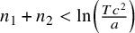 $n_1 + n_2 < \ln \left (\frac {T c^2}{a}\right )$
. Similarly,
 $$\begin{align*}c^2 \cdot T_0\cdot e^{-2} \cdot e^{-(n_1 + n_2)} \leq |x_1 x_2|y \leq b, \end{align*}$$
and thus
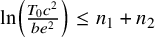 $\ln \left (\frac {T_0 c^2}{b e^2}\right ) \leq n_1 + n_2$
. In other words,
 $\Delta _{\Omega ,n}$
is nonempty only if
 $n \in \mathcal {F}_\Omega $
, and thus the union in (3.6) can without loss of generality be restricted to
 $\mathcal {F}_\Omega $
.
Finally, suppose that
 $(\underline {x},y) \in \Delta _{\Omega ,n}$
for some n. Then
 and
 $$\begin{align*}\frac{a}{c^2} < \frac{a}{|x_1 x_2|} < y \leq \frac{b}{|x_1 x_2|} \leq \frac{b e^2}{c^2}, \end{align*}$$
and thus

independently of n.
4 Group perturbations and controlled sets
The aim of this section is to establish regularity under small
 $\operatorname {SL}_3(\mathbb {R})$
-perturbations for families of sets as in (3.3). Since the sets relevant to our problem degenerate in some directions, we will need to introduce a new notion of regularity.
We begin with some notation. If
 $E \subset \mathbb {R}^2 \times \mathbb {R}$
, let
 $$\begin{align*}E^y = \{ \underline{x} \in \mathbb{R}^2 \, : \, (\underline{x},y) \in E \} \quad \text{and} \quad E_{\underline{x}} = \{ y \in \mathbb{R} \, : \, (\underline{x},y) \in E \}, \end{align*}$$
for
 $y \in \mathbb {R}$
and
 $\underline {x} \in \mathbb {R}^2$
. We refer to
 $E^y$
as the y-section of E, and to
 $E_{\underline {x}}$
as the
 $\underline {x}$
-section of E.
The following definition captures a convenient form of regularity that we will use in the paper.
Definition 4.1 (Controlled set)
Let
 $M> 1$
and
 $0 < \varepsilon < \gamma <M$
. We say that a Borel set
 $E \subset \mathbb {R}^2 \times \mathbb {R}$
is
 $(\varepsilon ,\gamma ,M)$
-controlled if either
 $$\begin{align*}E \subset [-M,M]^2 \times (\gamma,M] \quad \text{and} \quad \sup_{y \in [\gamma,1]} \operatorname{\mathrm{Vol}}_2(E^y) \ll_M \max\left(\varepsilon,-\frac{\varepsilon}{\gamma} \ln\left(\frac{\varepsilon}{\gamma}\right)\right), \end{align*}$$
or if there is an interval
 $[\alpha ,\beta ]$
such that
 $$\begin{align*}E \subset [-M,M]^2 \times [\alpha,\beta], \quad \beta-\alpha \ll_M \varepsilon,\quad \text{and} \quad \alpha\geq \gamma/2 \end{align*}$$
with implicit constants that are independent of
 $\varepsilon $
and
 $\gamma $
. If E satisfies the first set of conditions, we say that E is type I and if E satisfies the second set of conditions, we say that E is type II. We refer to the implicit constants above as the bounds for E.
Roughly speaking, a controlled set is type I if all of its y-sections have uniformly small volumes and it is type II if all of its
 $\underline {x}$
-sections have uniformly small volumes.
Remark 4.2. Note that if
 $\varepsilon < \gamma ' < \gamma $
,
 $\varepsilon /\gamma '<1/e$
and E is an
 $(\varepsilon ,\gamma ,M)$
-controlled set, then E is also an
 $(\varepsilon ,\gamma ',M)$
-controlled set.
Let
 $M>1$
. For the rest of this section, let us fix the following real parameters:
 $$ \begin{align} 0 < a < b \quad \text{and} \quad u_1^{-} < u_1^{+} \leq 1/2, u_2^{-} < u_2^{+} \leq 1/2 \quad \text{and} \quad 0<\gamma < \delta \leq M. \end{align} $$
We define the set
 $$ \begin{align} \Delta := \left\{ (\underline{x},y) \, : \, \begin{array}{c} a < |x_1 x_2| \cdot y \leq b \\[0.3cm] u_i^{-} < |x_i| \leq u_i^{+} \text{for } i=1,2 \\[0.3cm] \gamma \leq y <\delta \end{array} \right\} \subset \mathbb{R}^2 \times \mathbb{R}. \end{align} $$
We fix the
 $\max $
-norm on
 $\mathbb {R}^3$
and denote by
 $\|\cdot \|_{\text {op}}$
the operator norm on
 $\operatorname {SL}_3(\mathbb {R})$
induced by the
 $\max $
-norm, in particular,
 $$ \begin{align*}\|g\cdot \underline{x}\|_\infty\le \|g\|_{\text{op}}\cdot \|\underline{x}\|_\infty, \quad\text{for } g\in \operatorname{SL}_3(\mathbb{R}) \text{ and } \underline{x}\in \mathbb{R}^3 \end{align*} $$
For
 $\varepsilon> 0$
, we denote by
 $V_\varepsilon $
the symmetric open neighborhoods around the identity in
 $\operatorname {SL}_3(\mathbb {R})$
:
 $$ \begin{align} V_\varepsilon := \left\{ g \in \operatorname{SL}_3(\mathbb{R}) \, : \, \|g-\operatorname{\mathrm{id}}\|_{\text{op}} < \varepsilon\quad \text{and} \quad \|g^{-1}-\operatorname{\mathrm{id}}\|_{\text{op}} < \varepsilon \right\}. \end{align} $$
In other words,
 $$ \begin{align} \|g^{\pm 1}.(\underline{x},y) - (\underline{x},y)\|_\infty < \varepsilon \cdot \|(\underline{x},y)\|_\infty, \quad \text{for all } g \in V_\varepsilon \text{ and } (\underline{x},y) \in \mathbb{R}^2 \times \mathbb{R}. \end{align} $$
The following lemma is the main result of this section.
Lemma 4.3. Let
 $\Delta $
be as in (4.2) with the assumptions (4.1). Then, for every
 $$ \begin{align*}0 < \varepsilon < \min\left(1/(2M),\gamma/(2M),a/(M^2+1)\right), \end{align*} $$
there are
 $(\varepsilon ,\gamma /2,M+1)$
-controlled sets
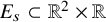 $E_s\subset \mathbb {R}^2 \times \mathbb {R}$
,
 $s=1,\ldots ,24$
, such that
 $$\begin{align*}\left(g^{-1}\Delta \setminus \Delta\right) \sqcup \left(\Delta \setminus g^{-1}\Delta\right) \subset \bigcup_{s} E_s\quad\text{for all } g \in V_\varepsilon. \end{align*}$$
Furthermore, the bounds in Definition 4.1 for the sets
 $E_s$
are independent of the parameters
 $a,b,u_{1}^{\pm },u_{2}^{\pm },\delta $
.
Proof. Let us fix
 $\varepsilon $
as above. For
 $g \in V_\varepsilon $
and
 $(\underline {x},y) \in \mathbb {R}^2 \times \mathbb {R}$
, we define
 $(\underline {x}(g),y(g))$
by
 $$ \begin{align} g.(\underline{x},y) := (\underline{x}(g),y(g)) = ({x}_1(g),x_2(g),y(g)). \end{align} $$
Then
 $$ \begin{align} \max(|x_1(g)-x_1|,|x_2(g)-x_2|,|y(g)-y|) < \varepsilon \cdot \|(\underline{x},y)\|_\infty, \end{align} $$
for all
 $(\underline {x},y) \in \mathbb {R}^2 \times \mathbb {R}$
. In particular, for
 $(\underline {x},y)\in \Delta $
,
 $$ \begin{align*}\max(|x_1(g)-x_1|,|x_2(g)-x_2|,|y(g)-y|) < M \varepsilon. \end{align*} $$
Hence, it follows that
 $$ \begin{align*}u_i^{-}-M\varepsilon < |x_i(g)| \leq u_i^{+}+M\varepsilon \text{for } i=1,2 \quad \text{and} \quad \gamma-M\varepsilon \leq y(g) \leq\delta+M\varepsilon. \end{align*} $$
Also using that
 $\varepsilon <1/(2M)$
,
 $$ \begin{align*} \big||x_1 x_2| \cdot y-|x_1(g) x_2(g)| \cdot y(g)\big| \le& \big||x_1 x_2| \cdot y -|x_1(g) x_2| \cdot y \big| +\big||x_1(g) x_2| \cdot y-|x_1(g) x_2(g)| \cdot y\big|\\ &+\big||x_1(g) x_2(g)| \cdot y-|x_1(g) x_2(g)| \cdot y(g)\big| \le \varepsilon M^2. \end{align*} $$
Therefore, we also have that
 $$ \begin{align*}a-\varepsilon M^2 < |x_1(g) x_2(g)| \cdot y(g) \leq b+\varepsilon M^2. \end{align*} $$
We conclude that for
 $g\in V_\varepsilon $
,
 $$ \begin{align*}g^{-1}\Delta\subset \Delta_\varepsilon^+, \end{align*} $$
where
 $$ \begin{align*}\Delta_\varepsilon^+ := \left\{ (\underline{x},y) \, : \, \begin{array}{c} a -\varepsilon M^2< |x_1 x_2| \cdot y \leq b +\varepsilon M^2\\[0.3cm] u_i^{-}(\varepsilon)< |x_i| \leq u_i^{+}(\varepsilon) \text{for } i=1,2 \\[0.3cm] \gamma -\varepsilon M \leq y <\delta+\varepsilon M \end{array} \right\}, \end{align*} $$
where
 $u_i^{-}(\varepsilon ):=u_i^{-} -\varepsilon M$
and
 $u_i^{+}(\varepsilon ):=u_i^{+} +\varepsilon M$
. We note that
 $$ \begin{align} \Delta_\varepsilon^+\subset (-1,1)^2\times [\gamma/2,M+1], \end{align} $$
because
 $\varepsilon <\gamma /(2M)$
and
 $\varepsilon <1/(2M)$
.
Let
 $$ \begin{align*}E_1:=\{(\underline{x},y)\in \Delta_\varepsilon^+: \, a-\varepsilon M^2<|x_1 x_2| \cdot y \le a\}. \end{align*} $$
For all
 $y>0$
,
 $$\begin{align*}E_{1}^y \subset \left( \begin{array}{ll} u_1^{+}(\varepsilon) & 0 \\ 0 & u_2^{+}(\varepsilon) \end{array} \right) \cdot \left(\Xi\left( \frac{a}{y \cdot u_1^{+}(\varepsilon) u_2^{+}(\varepsilon)} \right) \setminus \Xi\left( \frac{a-\varepsilon M^2}{y \cdot u_1^{+}(\varepsilon) u_2^{+}(\varepsilon)} \right) \right), \end{align*}$$
where the set
 $\Xi (\cdot )$
is defined as in (A.1). It follows from (A.3) that
 $$ \begin{align*} &\operatorname{\mathrm{Vol}}_2\left( \Xi\left( \frac{a}{y \cdot u_1^{+}(\varepsilon) u_2^{+}(\varepsilon)} \right) \setminus \Xi\left(\frac{a-\varepsilon M^2}{y \cdot u_1^{+}(\varepsilon) u_2^{+}(\varepsilon)}\right)\right)\\ \leq & -\frac{4\varepsilon M^2}{y \cdot u_1^{+}(\varepsilon) u_2^{+}(\varepsilon)} \cdot \ln^-\left (\frac{a-\varepsilon M^2}{y \cdot u_1^{+}(\varepsilon) u_2^{+}(\varepsilon)}\right), \end{align*} $$
where
 $\ln ^-(z):=\ln \min (1,z)$
. Since
 $\varepsilon < a/(M^2+1)$
and
 $u_1^+(\varepsilon ),u_2^+(\varepsilon )< 1$
, we have
 $$ \begin{align*}\frac{a-\varepsilon M^2}{u_1^{+}(\varepsilon)u_2^{+}(\varepsilon)}> \varepsilon, \end{align*} $$
and thus
 $$ \begin{align} \operatorname{\mathrm{Vol}}_2((E_{1})^y) \ll_M -\frac{\varepsilon}{y} \cdot \ln^-\left(\frac{\varepsilon}{y}\right) \ll -\frac{2\varepsilon}{\gamma} \cdot \ln^-\left(\frac{2\varepsilon}{\gamma}\right) \end{align} $$
for all
 $y\ge \gamma /2$
. This verifies that the set
 $E_1$
is
 $(\varepsilon ,\gamma /2,M+1)$
-controlled.
Let
 $$ \begin{align*}E_2:=\{(\underline{x},y)\in \Delta_\varepsilon^+: \, u_1^-(\varepsilon) < x_1\le u_1^-\}. \end{align*} $$
Then for all y,
 $$ \begin{align*}\operatorname{\mathrm{Vol}}_2((E_{1})^y)\le M\varepsilon, \end{align*} $$
so that this set is also
 $(\varepsilon ,\gamma /2,M+1)$
-controlled. The set
 $$ \begin{align*}E_3:=\{(\underline{x},y)\in \Delta_\varepsilon^+: \, \gamma-M\varepsilon \le y < \gamma\}. \end{align*} $$
is also obviously
 $(\varepsilon ,\gamma /2,M+1)$
-controlled of type II.
Finally, we observe that
 $\Delta _\varepsilon ^+\backslash \Delta =\Delta _\varepsilon ^+\cap \Delta ^c$
is contained in a union of of subsets of
 $\Delta _\varepsilon ^+$
, where each subset is defined by the negation of one of the inequalities that appears in the definition of
 $\Delta $
. Furthermore, in the case of
 ${x}_i$
,
 $i=1,2$
, we get two sets of inequalities
 $u_i^{-}(\varepsilon )< |x_i|\le u_i^-$
and
 $u_i^{+}< |x_i| \leq u_i^{+}(\varepsilon )$
which we view as four sets of inequalities in terms of
 ${x}_i$
and consider the four corresponding subsets. This way we obtain twelve sets
 $E_s$
. Since these sets are defined similarly to either
 $E_1$
,
 $E_2$
, or
 $E_3$
, we can analyze them as above. Therefore, we conclude that all
 $E_s$
’s are
 $(\varepsilon ,\gamma /2,M+1)$
-controlled. This verifies the claim of the lemma for the set
 $g^{-1}\Delta \backslash \Delta \subset \Delta _\varepsilon ^+\backslash \Delta $
.
To handle the set
 $\Delta \backslash g^{-1}\Delta $
, we observe that for
 $g\in V_\varepsilon $
,
 $$ \begin{align*}g^{-1}\Delta\supset \Delta_\varepsilon^-, \end{align*} $$
where
 $$ \begin{align*}\Delta_\varepsilon^- := \left\{ (\underline{x},y) \, : \, \begin{array}{c} a +\varepsilon M^2< |x_1 x_2| \cdot y \leq b -\varepsilon M^2\\[0.3cm] u_i^{-} +\varepsilon M< |x_i| \leq u_i^{+} -\varepsilon M\ \text{for } i=1,2 \\[0.3cm] \gamma +\varepsilon M \leq y <\delta-\varepsilon M \end{array} \right\}, \end{align*} $$
and
 $\Delta \backslash \Delta _\varepsilon ^-$
is contained in the union of twelve
 $(\varepsilon ,\gamma /2,M+1)$
-controlled sets. This can be verified as above, so that we omit the details.
5 Height function estimates
In this section we define a height function on the space
 $\widetilde {\mathcal {L}}_3$
consisting of all lattices in
 $\mathbb {R}^3$
and prove some technical level set estimates for this function that will be used later in our analysis of Siegel transforms.
Let
 $\widetilde {\mathcal {L}}_3$
denote the space of all lattices in
 $\mathbb {R}^3$
, endowed with the standard action of
 $\operatorname {GL}_3(\mathbb {R})$
. Given a bounded Borel function
 $f : \mathbb {R}^3 \rightarrow \mathbb {R}$
such that the set
 $\{ f \neq 0\}$
is bounded, we define the Siegel transform
 $\widehat {f} : \widetilde {\mathcal {L}_3} \rightarrow \mathbb {R}$
by
 $$\begin{align*}\widehat{f}(\Lambda) := \sum_{\underline{\lambda} \in \Lambda \setminus \{0\}} f(\underline{\lambda}), \quad \text{for } \Lambda \in \widetilde{\mathcal{L}_3}. \end{align*}$$
Let
 $\mathcal {L}_3 \subset \widetilde {\mathcal {L}}_3$
denote the subspace of all unimodular lattices. This subspace is preserved by the restricted
 $\operatorname {SL}_3(\mathbb {R})$
-action, and it is well-known that
 $\mathcal {L}_3$
carries a unique
 $\operatorname {SL}_3(\mathbb {R})$
-invariant Borel probability measure, which we denote by
 $\mu $
. The following classical theorem of Siegel will play an important role in our analysis.
Theorem 5.1 (Siegel’s theorem)
Let f be a bounded Borel function with compact support. Then
 $\widehat {f} \in L^1(\mu )$
and
 $$\begin{align*}\int_{\mathcal{L}_3} \widehat{f} \, d\mu = \int_{\mathbb{R}^3} f(\underline{z}) \, d\underline{z}, \end{align*}$$
where the volume measure on
 $\mathbb {R}^3$
has been normalized so that
 $\operatorname {\mathrm {Vol}}_3([0,1]^3) = 1$
.
5.1 A height function on
$\tilde {\mathcal {L}}_3$

Let
 $\{\underline {e}_1,\underline {e}_2,\underline {e}_3\}$
denote the standard (ordered) basis of
 $\mathbb {R}^3$
. We extend the
 $\max $
-norm with respect to this basis to the second exterior power
 $\mathbb {R}^3 \wedge \mathbb {R}^3$
as follows. If
 $\underline {u}, \underline {v} \in \mathbb {R}^3$
and
 $$\begin{align*}w = \underline{u} \wedge \underline{v} = w_{12} \, \underline{e}_1 \wedge \underline{e}_2 + w_{13} \, \underline{e}_1 \wedge \underline{e}_3 + w_{23} \, \underline{e}_2 \wedge \underline{e}_3, \end{align*}$$
then
 $\|w\|_\infty = \max (|w_{12}|,|w_{13}|,|w_{23}|)$
.
Let
 $\Lambda $
be a (not necessarily unimodular) lattice in
 $\mathbb {R}^3$
. We define the functions
 $$ \begin{align*} s_1(\Lambda) &:= \inf\left\{ \|\underline{\lambda}\|_\infty \, : \, \underline{\lambda} \in \Lambda \setminus \{0\} \right\}, \\[0.2cm] s_2(\Lambda) &:= \inf\left\{ \|\underline{\lambda}_1 \wedge \underline{\lambda}_2\|_\infty \, : \, \underline{\lambda}_1 \wedge \underline{\lambda}_2 \neq 0, \underline{\lambda}_1,\underline{\lambda}_2 \in \Lambda \setminus \{0\} \right\}, \\[0.2cm] s_3(\Lambda) &:= \inf\left\{ |\alpha| \, : \, \alpha \, \underline{e}_1 \wedge \underline{e}_2 \, \wedge \underline{e}_3 = \underline{\lambda}_1 \wedge \underline{\lambda}_2 \wedge \underline{\lambda}_3 \neq 0, \underline{\lambda}_1,\underline{\lambda}_2, \underline{\lambda}_3 \in \Lambda \setminus \{0\} \right\}, \end{align*} $$
and the height function
 $$ \begin{align} \operatorname{\mathrm{ht}}(\Lambda) := \min\big(s_1(\Lambda),s_2(\Lambda),s_3(\Lambda)\big)^{-1}. \end{align} $$
Since
 $$\begin{align*}\|g\cdot\underline{w}\|_\infty \leq \|g\|_{\text{op}} \cdot \|\underline{w}\|_\infty \quad \text{and} \quad \|g\cdot \underline{w}\|_\infty \geq \|g^{-1}\|^{-1}_{\text{op}} \cdot \|\underline{w}\|_\infty, \end{align*}$$
for all
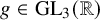 $g \in \operatorname {GL}_3(\mathbb {R})$
and
 $\underline {w} \in \mathbb {R}^3$
(where
 $\|\cdot \|_{\text {op}}$
denotes the operator norm with respect to the
 $\max $
-norm on
 $\mathbb {R}^3$
), we have
 $$ \begin{align} \|g\|^{-1}_{\text{op}} \cdot \operatorname{\mathrm{ht}}(\Lambda) \leq \operatorname{\mathrm{ht}}(g.\Lambda) \leq \|g^{-1}\|_{\text{op}}\cdot \operatorname{\mathrm{ht}}(\Lambda), \end{align} $$
for all
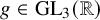 $g \in \operatorname {GL}_3(\mathbb {R})$
and
 $\Lambda \in \widetilde {\mathcal {L}}_3$
. Before we proceed to the main topic of this section, we recall an important inequality due to Schmidt [Reference Schmidt18, Lemma 2].
Lemma 5.2. For every bounded Borel function with compact support,
 $$\begin{align*}|\widehat{f}(\Lambda)| \ll_{\operatorname{\mathrm{supp}}(f)} \|f\|_\infty \cdot \operatorname{\mathrm{ht}}(\Lambda), \quad \text{for all } \Lambda \in \widetilde{\mathcal{L}}_3, \end{align*}$$
where the implicit constants only depend on
 $\operatorname {\mathrm {supp}}(f)$
.
5.2 Main results
We recall that
 $$\begin{align*}a(t) = \left( \begin{matrix} e^{t_1} & & \\ & e^{t_2} & \\ & & e^{-(t_1 + t_2)} \end{matrix} \right), \quad \text{for } t = (t_1,t_2) \in \mathbb{R}_{+}^2. \end{align*}$$
Given
 $\underline {x} =({x}_1,x_2)\in \mathbb {R}^2$
and
 $r> 0$
, we define the lattice
 $$ \begin{align} \Lambda_{\underline{x},r} := \left\{ \underline{p} + q(\iota(\underline{x}) + r \underline{e}_3) \, : \, \underline{p} \in \operatorname{\mathrm{span}}_{\mathbb{Z}}(\underline{e}_1,\underline{e}_2), q \in \mathbb{Z} \right\}, \end{align} $$
where
 $\iota (\underline {x}):=({x}_1,x_2,0)$
. We note that
 $\Lambda _{\underline {x},r}$
is a unimodular lattice if and only if
 $r = 1$
.
Our first theorem in this section provides uniform upper bounds of the height function along
 $a(t)$
-orbits of lattices of the form
 $\Lambda _{\underline {x},r}$
. Here and later in the paper, we use the notation
 $$ \begin{align*}\lfloor t \rfloor:=\min(t_1,t_2)\quad\text{for } t=(t_1,t_2)\in\mathbb{R}^2_{+}. \end{align*} $$
Theorem 5.3. For all
 $r>0$
and
 $t = (t_1,t_2) \in \mathbb {R}^2_{+}$
,
 $$\begin{align*}\sup\left\{ \operatorname{\mathrm{ht}}(a(t)\Lambda_{\underline{x},r}) \, : \, \underline{x} \in [0,1)^2 \right\} \leq \max\left(e^{t_1 + t_2}/r,e^{-\lfloor t \rfloor} \right). \end{align*}$$
Our second theorem roughly tells us that the map
 $t \mapsto \operatorname {\mathrm {ht}}(a(t)\Lambda _{\underline {x},r})$
is not large on a big volume set.
Theorem 5.4. For every
 $r>0$
,
 $L> \max (1,1/r)$
and
 $t \in \mathbb {R}^2_{+}$
,
 $$\begin{align*}\operatorname{\mathrm{Vol}}_2\left( \left\{ \underline{x} \in [0,1)^2 \, : \, \operatorname{\mathrm{ht}}(a(t)\Lambda_{\underline{x},r}) \geq L \right\}\right) \ll \max(r^{-1},r^{-2})L^{-3} + r^{-1}L^{-2} e^{-\lfloor t \rfloor} , \end{align*}$$
where the implicit constants are independent of
 $L, r$
and t.
The theorems above provide useful upper bounds on certain integrals involving the height functions restricted to super-level sets. To state these bounds, we define the sets
 $$ \begin{align} M_{t,r}(\eta) := \left\{ \underline{x} \in [0,1)^2 \, : \, \operatorname{\mathrm{ht}}(a(t)\Lambda_{\underline{x},r}) \geq \eta \right\} \end{align} $$
for
 $\eta \geq 0$
. We then have the following corollary, which we prove at the end of this section:
Corollary 5.5. Let
 $\rho>0$
and
 $\theta : [0,\infty ) \rightarrow [0,\infty )$
be an increasing measurable function such that
 $u \mapsto \frac {\theta (u)}{u^2}$
is decreasing on
 $[1,\infty )$
. Then, for every
 $t\in \mathbb {R}^2_+$
,
 $r>\rho $
and
 $\eta \ge e^{2}\rho ^{-1}$
, we have
 $$\begin{align*}\int_{M_{t,r}(\eta)} \theta(\operatorname{\mathrm{ht}}(a(t)\Lambda_{\underline{x},r})) \, d\underline{x} \ll \left( \max(r^{-1},r^{-2}) \eta^{-1} + r^{-1}e^{-\lfloor t \rfloor} \right) \cdot \int_{ e^{-2}\eta}^{e^{t_1 + t_2 + 1}\max(1,\rho^{-1})} \frac{\theta(u)}{u^3} \, du, \end{align*}$$
where the implicit constants are independent of
 $\rho , \eta , r$
and t.
5.3 Lemmas about heights
Lemma 5.6 (Uniform Lower Bound for
$s_{1}$
)

For all
 $r>0$
and
 $t = (t_1,t_2) \in \mathbb {R}^2_{+}$
,
 $$\begin{align*}\inf\left\{ s_1(a(t)\Lambda_{\underline{x},r}) \, : \, \underline{x} \in [0,1)^2 \right\} \geq \min\left(e^{\lfloor t \rfloor}, r \cdot e^{-(t_1 + t_2)}\right). \end{align*}$$
Proof. Let
 $\underline {x} = ({x}_1,x_2) \in [0,1)^2$
,
 $r> 0$
, and
 $t = (t_1,t_2) \in \mathbb {R}^2_{+}$
. We note that for every
 $\underline {p} = (p_1,p_2) \in \mathbb {Z}^2$
and
 $q \in \mathbb {Z}$
, we have
 $$\begin{align*}\|a(t)(\underline{p} + q(\iota(\underline{x})+r\underline{e}_3))\|_\infty = \max\left(e^{t_1} \cdot |p_1 + qx_1|, e^{t_2} \cdot |p_2 + qx_2|, r \cdot |q| \cdot e^{-(t_1+t_2)}\right). \end{align*}$$
We assume that
 $\underline {p} + q(\iota (\underline {x})+r\underline {e}_3) \neq 0$
. If
 $q = 0$
, then
 $\underline {p} \neq 0$
, and thus
 $$\begin{align*}\|a(t)(\underline{p} + q(\iota(\underline{x})+r\underline{e}_3))\|_\infty \geq e^{\lfloor t \rfloor}. \end{align*}$$
If
 $q \neq 0$
, then
 $$\begin{align*}\|a(t)(\underline{p} + q(\iota(\underline{x})+r\underline{e}_3))\|_\infty \geq r \cdot e^{-(t_1 + t_2)}. \end{align*}$$
We get a uniform lower bound by taking the minimum of these two bounds.
Lemma 5.7 (Volume Bound for
$s_{1}$
)

For every
 $0 < \varepsilon < 1$
,
 $r>0$
and
 $t \in \mathbb {R}^2_{+}$
, we have
 $$\begin{align*}\operatorname{\mathrm{Vol}}_2\left(\left\{ \underline{x} \in [0,1)^2 \, : \, s_{1}(a(t)\Lambda_{\underline{x},r}) \leq \varepsilon \right\}\right) \ll \frac{\varepsilon^3}{r}, \end{align*}$$
where the implicit constants are independent of
 $\varepsilon , r$
and t.
Proof. Let
 $0 < \varepsilon < 1$
and
 $r>0$
and
 $t = (t_1,t_2) \in \mathbb {R}^2_{+}$
. Pick
 $\underline {x}=({x}_1,x_2) \in [0,1)^2$
such that
 $$\begin{align*}s_{1}(a(t)\Lambda_{\underline{x},r}) \leq \varepsilon. \end{align*}$$
This means that we can find a nonzero vector
 $\underline {p} + q (\iota (\underline {x}) + r\underline {e}_3) \in \Lambda _{\underline {x},r}$
such that
 $$\begin{align*}\Lambda_{\underline{x}}(t) := e^{t_1}(p_1 + qx_1) \, \underline{e}_1 + e^{t_2}(p_2 + qx_2) \, \underline{e}_2 + r e^{-(t_1 + t_2)}q \, \underline{e}_3\in a(t)\Lambda_{\underline{x},r} \end{align*}$$
satisfies
 $\|\Lambda _{\underline {x}}(t)\|_\infty \leq \varepsilon $
. Writing this information coordinate-wise, we get the inequalities
 $$ \begin{align} |p_1 + qx_1| \leq \varepsilon \cdot e^{-t_1}, |p_2 + qx_2| \leq \varepsilon \cdot e^{-t_2}, |q| \leq \frac{\varepsilon \cdot e^{t_1 + t_2}}{r}. \end{align} $$
Since
 $\varepsilon < 1$
and
 $t_1, t_2 \geq 0$
, there are no nonzero solutions for p when
 $q = 0$
.
For
 $q \neq 0$
, we note that since
 $\underline {x} = ({x}_1,x_2) \in [0,1)^2$
, there are at most
 $O(q^2)$
choices for
 $\underline {p} = (p_1,p_2) \in \mathbb {Z}^2$
. Furthermore, for each such choice of
 $\underline {p}$
,
 $$\begin{align*}\operatorname{\mathrm{Vol}}_2\left( \left\{ \underline{x} \in [0,1)^2 \, : \, |p_1 + qx_1| \leq \varepsilon \cdot e^{-t_1}, |p_2 + qx_2| \leq \varepsilon \cdot e^{-t_2} \right\}\right) \ll \frac{\varepsilon^2 \cdot e^{-(t_1 + t_2)}}{q^2}, \end{align*}$$
where the implicit constants are independent of
 $\underline {p}$
,
 $\varepsilon $
and t. In particular, upon summing over all possible
 $\underline {p}$
and q, we see that the volume of the set of
 $\underline {x} \in [0,1)^2$
for which the inequalities in (5.5) are satisfied is bounded from above by
 $O( \varepsilon ^3/r)$
, which finishes the proof.
Let us introduce some notation which will be used in the proofs below. Given
 $$\begin{align*}r> 0, \underline{x} \in [0,1)^2, \underline{p}^{(1)}, \underline{p}^{(2)} \in \operatorname{\mathrm{span}}_{\mathbb{Z}}(\underline{e}_1,\underline{e}_2), q_1,q_2 \in \mathbb{Z}, \end{align*}$$
define
 $\underline {v}_1, \underline {v}_2 \in \Lambda _{\underline {x},r}$
by
 $$ \begin{align} \underline{v}_1 := \underline{p}^{(1)} + q_1(\iota(\underline{x}) + r\underline{e}_3) \quad \text{and} \quad \underline{v}_2 := \underline{p}^{(2)} + q_2(\iota(\underline{x}) + r\underline{e}_3). \end{align} $$
Furthermore, given
 $t = (t_1,t_2) \in \mathbb {R}^2$
, we define
 $$ \begin{align*} \omega_{\underline{x}}(t) &:= a(t)\left(\left( \underline{p}^{(1)} + q_1(\iota(\underline{x}) + r\underline{e}_3) \right) \wedge \left( \underline{p}^{(2)} + q_2(\iota(\underline{x}) + r\underline{e}_3) \right)\right) \\[0.2cm] &= a(t)\left(\underline{p}^{(1)} \wedge \underline{p}^{(2)} + \left(q_2 \underline{p}^{(1)} - q_1 \underline{p}^{(2)}\right) \wedge \underline{x} + r \left(q_2 \underline{p}^{(1)} - q_1 \underline{p}^{(2)}\right) \wedge \underline{e}_3\right). \end{align*} $$
Note that
 $$\begin{align*}\omega_{\underline{x}}(t) = e^{t_1 + t_2 } \, \omega_{1,2}(\underline{x}) \, \underline{e}_1 \wedge \underline{e}_2 + r \, e^{-t_2}w_1 \, \underline{e}_1 \wedge \underline{e}_3 + r \, e^{-t_1} \, w_2 \, \underline{e}_2 \wedge \underline{e}_3, \end{align*}$$
where
 $$\begin{align*}\omega_{1,2}(\underline{x}) = m(\underline{p}) + (w_1 x_2 - w_2 x_1) \quad \text{and} \quad \underline{w} = w_1 \underline{e}_1 + w_2 \underline{e}_2 = q_2 \underline{p}^{(1)} - q_1 \underline{p}^{(2)}, \end{align*}$$
and
 $m(\underline {p})$
is the unique integer such that
 $\underline {p}^{(1)} \wedge \underline {p}^{(2)} = m(\underline {p}) \, \underline {e}_1 \wedge \underline {e}_2$
. In particular,
 $$ \begin{align} \|\omega_{\underline{x}}(t)\|_\infty = \max\left(e^{t_1 + t_2} \cdot |m(\underline{p}) + (w_1 x_2 - w_2 x_1)|, e^{-t_2} \cdot r \cdot |w_1|, e^{-t_1} \cdot r \cdot |w_2| \right). \end{align} $$
Note that if
 $\underline {v}_1$
and
 $\underline {v}_2$
are linearly independent, then
 $\omega _{\underline {x}}(t) \neq 0$
, and thus either
 $\underline {w} \neq 0$
or
 $m(\underline {p}) \neq 0$
.
Lemma 5.8 (Uniform Lower Bound for
$s_{2}$
)

For all
 $r>0$
and
 $t = (t_1,t_2) \in \mathbb {R}^2_{+}$
,
 $$\begin{align*}\inf\left\{ s_2(a(t)\Lambda_{\underline{x},r}) \, : \, \underline{x} \in [0,1)^2 \right\} \geq \min\left(r \cdot e^{-\lfloor t \rfloor},e^{t_1 + t_2}\right). \end{align*}$$
Proof. Note that
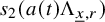 $s_2(a(t)\Lambda _{\underline {x},r})$
is the minimum of
 $\|\omega _{\underline {x}}(t)\|_\infty $
, when
 $\underline {v}_1$
and
 $\underline {v}_2$
, defined as in (5.6), vary over all linearly independent pairs of vectors in
 $\Lambda _{\underline {x},r}$
. Hence, by (5.7), we need lower bounds on
 $$\begin{align*}\max\left(e^{t_1 + t_2} \cdot |m(\underline{p}) + (w_1 x_2 - w_2 x_1)|, e^{-t_2} \cdot r \cdot |w_1|, e^{-t_1} \cdot r \cdot |w_2| \right), \end{align*}$$
when either
 $\underline {w} \neq 0$
or
 $m(\underline {p}) \neq 0$
. If
 $\underline {w} \neq 0$
, then since
 $w_1$
and
 $w_2$
are integers, we have
 $$\begin{align*}\max\left(e^{t_1 + t_2} \cdot |m(\underline{p}) + (w_1 x_2 - w_2 x_1)|, e^{-t_2} \cdot r \cdot |w_1|, e^{-t_1} \cdot r \cdot |w_2| \right) \geq r \cdot e^{-\lfloor t \rfloor}, \end{align*}$$
and if
 $m(\underline {p}) \neq 0$
and
 $\underline {w}=0$
, then
 $$\begin{align*}\max\left(e^{t_1 + t_2} \cdot |m(\underline{p}) + (w_1 x_2 - w_2 x_1)|, e^{-t_2} \cdot r \cdot |w_1|, e^{-t_1} \cdot r \cdot |w_2| \right) \geq e^{t_1 + t_2}. \end{align*}$$
We get a uniform lower bound by taking the minimum of these two bounds.
Lemma 5.9 (Volume Bound for
$s_{2}$
)

For every
 $0 < \varepsilon < 1$
,
 $r>0$
and
 $t \in \mathbb {R}^2_{+}$
, we have
 $$\begin{align*}\operatorname{\mathrm{Vol}}_2\left(\left\{ \underline{x} \in [0,1)^2 \, : \, s_{2}(a(t)\Lambda_{\underline{x},r}) \leq \varepsilon \right\}\right) \ll \frac{\varepsilon^3}{r^2} +\frac{\varepsilon^2 \cdot e^{-\lfloor t \rfloor}}{r}, \end{align*}$$
where the implicit constants are independent of
 $\varepsilon , r$
and t.
Proof. Let
 $0 < \varepsilon < 1$
,
 $r>0$
and
 $t = (t_1,t_2) \in \mathbb {R}^2_{+}$
. Pick
 $\underline {x} \in [0,1)^2$
such that
 $$\begin{align*}s_{2}(a(t)\Lambda_{\underline{x},r}) \leq \varepsilon. \end{align*}$$
This means that we can find two linearly independent vectors
 $\underline {v}_1$
and
 $\underline {v}_2$
as in (5.6) such that
 $\|\omega _{\underline {x}}(t)\|_\infty \leq \varepsilon $
. By (5.7), this results in the bounds
 $$ \begin{align} |m(\underline{p}) + (w_1 x_2 - w_2 x_1)| \leq \varepsilon \cdot e^{-(t_1+t_2)}, |w_1| \leq \frac{\varepsilon \cdot e^{t_2}}{r}, |w_2| \leq \frac{\varepsilon \cdot e^{t_1}}{r}. \end{align} $$
We make two observations:
-
○ If
$q_1 = q_2 = 0$
, then
$\underline {w} = 0$
and
$|m(\underline {p})| \leq \varepsilon \cdot e^{-(t_1+t_2)}$
. Since
$\varepsilon < 1$
and
$t_1, t_2 \geq 0$
and
$m(\underline {p})$
is an integer, we must have
$m(\underline {p}) = 0$
. This readily implies that
$\underline {p}^{(1)} \wedge \underline {p}^{(2)} = 0$
, so
$\underline {p}^{(1)}$
and
$\underline {p}^{(2)}$
are linearly dependent, and thus
$\underline {v}_1$
and
$\underline {v}_2$
are linearly dependent as well, contrary to our assumption. -
○ If
$\underline {w} = 0$
and
$(q_1,q_2) \neq (0,0)$
, then
$q_2 \underline {v}_1 - q_1 \underline {v}_2 = 0$
, which contradicts our assumption that
$\underline {v}_1$
and
$\underline {v}_2$
are linearly independent.





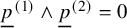






We can thus without loss of generality assume that
 $\underline {w} \neq 0$
and
 $(q_1,q_2) \neq (0,0)$
.
For a fixed
 $\underline {w} \neq 0$
and
 $m(\underline {p}) \in \mathbb {Z}$
, we have
 $$\begin{align*}\operatorname{\mathrm{Vol}}_2\left(\left\{ \underline{x} \in [0,1)^2 \, : \, |m(\underline{p}) + (w_1 x_2 - w_2 x_1)| \leq \varepsilon \cdot e^{-(t_1+t_2)} \right\}\right) \ll \frac{\varepsilon \cdot e^{-(t_1 + t_2)}}{\max(|w_1|,|w_2|)}, \end{align*}$$
where the implicit constants are independent of
 $\underline {p}$
and t. Furthermore, since
 $0<\varepsilon <1$
and
 $t_1,t_2\ge 0$
, it follows from (5.8) that there are at most
 $O\big (\max (|w_1|,|w_2|)\big )$
choices for
 $m(\underline {p})$
. We also note from (5.8) that there are
-
○
$O\left (\frac {\varepsilon ^2 \cdot e^{t_1+t_2}}{r^2}\right )$
choices for
$\underline {w}$
with
$w_1, w_2 \neq 0$
, -
○
$O\left (\frac {\varepsilon \cdot e^{t_2}}{r}\right )$
choices for
$\underline {w}$
with
$w_2 = 0$
, -
○
$O\left (\frac {\varepsilon \cdot e^{t_1}}{r}\right )$
choices for
$\underline {w}$
with
$w_1 = 0$
.


Summing over all of these choices, we get
 $$ \begin{align*} \operatorname{\mathrm{Vol}}_2\left(\left\{ \underline{x} \in [0,1)^2 \, : \, s_{2}(a(t)\Lambda_{\underline{x},r}) \leq \varepsilon \right\}\right) \ll \frac{\varepsilon^3}{r^2} + \frac{\varepsilon^2 \cdot e^{-t_1}}{r} + \frac{\varepsilon^2 \cdot e^{-t_2}}{r}, \end{align*} $$
which implies the claim.
Finally, we note the following elementary result for
 $s_3$
, whose proof is left to the reader.
Lemma 5.10. For all
 $t \in \mathbb {R}^2_{+}$
and
 $r> 0$
,
 $$\begin{align*}s_3(a(t)\Lambda_{\underline{x},r}) = r, \quad \text{for all } \underline{x} \in [0,1)^2. \end{align*}$$
5.4 Proof of Theorem 5.3
By Lemma 5.6, Lemma 5.8 and Lemma 5.10, we have
 $$ \begin{align*} \min(s_1(a(t)\Lambda_{\underline{x},r}),s_2(a(t)\Lambda_{\underline{x},r}),s_3(a(t)\Lambda_{\underline{x},r})) &\geq \min\left(e^{\lfloor t \rfloor}, r \cdot e^{-(t_1 + t_2)} ,r \cdot e^{-\lfloor t \rfloor},e^{t_1 + t_2},r\right)\\[0.2cm] &\geq \min\left(r \cdot e^{-(t_1 + t_2)},e^{\lfloor t \rfloor}\right), \end{align*} $$
for all
 $t = (t_1,t_2) \in \mathbb {R}^2_{+}$
. Hence,
 $$\begin{align*}\operatorname{\mathrm{ht}}(a(t)\Lambda_{\underline{x},r}) \leq \max\left(e^{t_1 + t_2}/r,e^{-\lfloor t \rfloor} \right), \end{align*}$$
for all
 $\underline {x} \in [0,1)^2$
.
5.5 Proof of Theorem 5.4
Let
 $L> 1$
. We first note that
 $$ \begin{align*} \operatorname{\mathrm{Vol}}_2\left( \left\{ \underline{x} \in [0,1)^2 \, : \, \operatorname{\mathrm{ht}}(a(t)\Lambda_{\underline{x},r}) \geq L \right\} \right) &= \operatorname{\mathrm{Vol}}_2\left( \bigcup_{i=1}^3 \left\{ \underline{x} \in [0,1)^2 \, : \, s_i(a(t)\Lambda_{\underline{x},r}) \leq \frac{1}{L}\right\} \right) \\[0.2cm] &\leq \sum_{i=1}^3 \operatorname{\mathrm{Vol}}_2\left(\left\{ \underline{x} \in [0,1)^2 \, : \, s_i(a(t)\Lambda_{\underline{x},r}) \leq \frac{1}{L}\right\} \right). \end{align*} $$
By Lemma 5.7 and Lemma 5.9 (applied with
 $\varepsilon = \frac {1}{L}$
), we have
 $$ \begin{align*} &\operatorname{\mathrm{Vol}}_2\left(\left\{ \underline{x} \in [0,1)^2 \, : \, s_1(a(t)\Lambda_{\underline{x},r}) \leq \frac{1}{L}\right\} \right) \ll \frac{1}{r L^3}, \end{align*} $$
and
 $$ \begin{align*} &\operatorname{\mathrm{Vol}}_2\left(\left\{ \underline{x} \in [0,1)^2 \, : \, s_2(a(t)\Lambda_{\underline{x},r}) \leq \frac{1}{L}\right\} \right) \ll \frac{1}{r^2 L^3} + \frac{e^{-\lfloor t \rfloor}}{rL^2}. \end{align*} $$
Furthermore, by Lemma 5.10, the last set in the sum is empty if
 $L> \frac {1}{r}$
. Combining these estimates, we obtain the theorem.
5.6 Proof of Corollary 5.5
Let
 $r>\rho $
and
 $t \in \mathbb {R}^2_{+}$
. We introduce the sets
 $$\begin{align*}B_{t,r}(i) = \left\{ \underline{x} \in [0,1)^2 \, : \, e^{i-1} < \operatorname{\mathrm{ht}}(a(t)\Lambda_{\underline{x},r}) \leq e^i \right\}, \quad \text{for } i \in \mathbb{Z}. \end{align*}$$
By Theorem 5.3,
 $$\begin{align*}\operatorname{\mathrm{ht}}(a(t)\Lambda_{\underline{x},r}) \leq \max\left(\frac{e^{t_1 + t_2}}{r},e^{-\lfloor t \rfloor} \right) \leq \max(1,\rho^{-1})e^{t_1 + t_2}, \quad \text{for all } \underline{x} \in [0,1)^2, \end{align*}$$
and thus
 $B_{t,r}(i)$
is empty for
 $i \geq t_1 + t_2 +\ln \max (1,\rho ^{-1})+ 1$
. Furthermore, by Theorem 5.4, applied with
 $L = e^{i-1}$
for
 $i \geq \ln (\rho ^{-1})+1$
, we have
 $$\begin{align*}\operatorname{\mathrm{Vol}}_2(B_{t,r}(i)) \ll \max(r^{-1},r^{-2}) e^{-3i}+ r^{-1}e^{-\lfloor t\rfloor}e^{-2i}. \end{align*}$$
Hence, since
 $\theta $
is increasing, for
 $\eta \ge e^{2}\rho ^{-1}$
,
 $$ \begin{align*} \int_{M_{t,r}(\eta)} \theta(\operatorname{\mathrm{ht}}(a(t)\Lambda_{\underline{x},r})) \, d\underline{x} \leq & \sum_{i = \lfloor \ln(\eta) \rfloor}^{\lceil t_1 + t_2+\ln\max(1,\rho^{-1}) \rceil} \theta(e^i) \cdot \operatorname{\mathrm{Vol}}_2(B_{t,r}(i)) \\[0.2cm] \ll & \max(r^{-1},r^{-2}) \left( \sum_{i=\lfloor \ln(\eta) \rfloor}^{\lceil t_1 + t_2+\ln\max(1,\rho^{-1}) \rceil} \theta(e^i) \cdot e^{-3i} \right) \\[0.2cm] &+ r^{-1} \cdot \left( \sum_{i=\lfloor \ln(\eta) \rfloor}^{\lceil t_1 + t_2 +\ln\max(1,\rho^{-1}) \rceil} \theta(e^i) \cdot e^{-2i} \right) \cdot e^{-\lfloor t \rfloor}. \end{align*} $$
By assumption,
 $u \mapsto \frac {\theta (u)}{u^2}$
is decreasing for
 $u \geq 1$
, and thus
 $$\begin{align*}\sum_{i=\lfloor \ln(\eta) \rfloor}^{\lceil t_1 + t_2+\ln\max(1,\rho^{-1}) \rceil} \theta(e^i) \cdot e^{-2i} \leq \int_{\lfloor \ln(\eta) \rfloor-1}^{t_1 + t_2+\ln\max(1,\rho^{-1}) + 1} \frac{\theta(e^u)}{e^{2u}} \, du \leq \int_{ e^{-2}\eta}^{e^{t_1 + t_2 + 1}\max(1,\rho^{-1})} \frac{\theta(u)}{u^3} \, du. \end{align*}$$
Also, in the summation range, we have
 $$\begin{align*}\sum_{i=\lfloor \ln(\eta) \rfloor}^{\lceil t_1 + t_2+\ln\max(1,\rho^{-1}) \rceil} \theta(e^i) \cdot e^{-3i} \ll \eta^{-1} \cdot \int_{ e^{-2}\eta}^{e^{t_1 + t_2 + 1}\max(1,\rho^{-1})} \frac{\theta(u)}{u^3} \, du. \end{align*}$$
We conclude that
 $$\begin{align*}\int_{M_{t,r}(\eta)} \theta(\operatorname{\mathrm{ht}}(a(t)\Lambda_{\underline{x},r})) \, d\underline{x} \ll \left( \max(r^{-1},r^{-2}) \eta^{-1} + r^{-1}e^{-\lfloor t \rfloor} \right) \cdot \int_{ e^{-2}\eta}^{e^{t_1 + t_2 + 1}\max(1,\rho^{-1})} \frac{\theta(u)}{u^3} \, du, \end{align*}$$
which finishes the proof.
6 Correlations between the number of shifted lattice points in boxes
If
 $B \subset \mathbb {R}^2$
is a bounded Borel set, we define the counting function
 $$ \begin{align} N_B(\underline{x}) = \left|\left(\mathbb{Z}^2 + \underline{x}\right) \cap B\right|, \quad \text{for } \underline{x} \in \mathbb{R}^2. \end{align} $$
Note that
 $N_B$
is
 $\mathbb {Z}^2$
-periodic, and thus completely determined by its values on
 $[0,1)^2$
.
Our main result in this section reads as follows.
Lemma 6.1. Let
 $M> 0$
and let
 $D^{(1)}$
and
 $D^{(2)}$
be Borel subsets of the square
 . Let
 $t = (t_1,t_2) \in \mathbb {R}^2_{+}$
with
 $t_1 \leq t_2$
and define
 $$\begin{align*}D^{(i)}_t = \left( \begin{matrix} e^{-t_1} & 0 \\ 0 & e^{-t_2} \end{matrix} \right) D^{(i)} \quad \text{for } i=1,2. \end{align*}$$
Then, for all
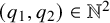 $(q_1,q_2) \in \mathbb {N}^2$
,
 $$\begin{align*}\int_{[0,1)^2} N_{D^{(1)}_t}(q_1\underline{x}) N_{D^{(2)}_t}(q_2\underline{x}) \, d\underline{x} \leq F_t\left( \frac{\max(q_1,q_2)}{\gcd(q_1,q_2)} \right) \cdot \max\left(\operatorname{\mathrm{Vol}}_2(D^{(1)}),\operatorname{\mathrm{Vol}}_2(D^{(2)})\right), \end{align*}$$
where
 $F_t$
is defined as in (B.3).
We will derive Lemma 6.1 from the following general result.
Lemma 6.2. Let
 $B_1$
and
 $B_2$
be bounded Borel sets in
 $\mathbb {R}^2$
and let
 $q_1$
and
 $q_2$
be relatively prime positive integers. Then,
 $$\begin{align*}\int_{[0,1)^2} N_{B_1}(q_1 \underline{x}) N_{B_2}(q_2 \underline{x}) \, d\underline{x} \leq \left| \mathbb{Z}^2 \cap \left(q_2 B_1 - q_1 B_2\right) \right| \cdot \min\left( \frac{\operatorname{\mathrm{Vol}}_2(B_1)}{q_1^2},\frac{\operatorname{\mathrm{Vol}}_2(B_2)}{q_2^2} \right). \end{align*}$$
Proof. Note that
 $\mathbb {Z}^2 \times \mathbb {Z}^2 = \bigsqcup _{\underline {k} \in \mathbb {Z}^2} E_{\underline {k}}(q_1,q_2)$
, where
 $$\begin{align*}E_{\underline{k}}(q_1,q_2) := \big\{ (\underline{p}_1,\underline{p}_2) \in \mathbb{Z}^2 \times \mathbb{Z}^2 \, : \, q_2 \underline{p}_1 - q_1 \underline{p}_2 = \underline{k} \big\}, \quad \text{for } \underline{k} \in \mathbb{Z}^2. \end{align*}$$
Hence,
 $$ \begin{align*} \int_{[0,1)^2} N_{B_1}(q_1\underline{x}) \, N_{B_2}(q_2\underline{x}) \, d\underline{x} &= \sum_{\underline{p}_1, \underline{p}_2} \int_{[0,1)^2} \chi_{B_1}(\underline{p}_1 + q_1 \underline{x}) \, \chi_{B_2}(\underline{p}_2 + q_2 \underline{x}) \, d\underline{x} \\[0.2cm] &= \sum_{\underline{k}} C_{\underline{k}}(q_1,q_2), \end{align*} $$
where
 $C_{\underline {k}}(q_1,q_2) := \sum _{(\underline {p}_1,\underline {p}_2) \in E_{\underline {k}}(q_1,q_2)} \int _{[0,1)^2} \chi _{B_1}(\underline {p}_1 + q_1 \underline {x}) \, \chi _{B_2}(\underline {p}_2 + q_2 \underline {x}) \, d\underline {x}$
.
Fix
 $\underline {k} \in \mathbb {Z}^2$
and
 $(\underline {p}_1',\underline {p}_2') \in E_{\underline {k}}(q_1,q_2)$
. Then,
 $$ \begin{align} E_{\underline{k}}(q_1,q_2) = \left\{ \left(\underline{p}_1' + q_1\underline{l},\underline{p}_2' + q_2 \underline{l}\right) \, : \, \underline{l} \in \mathbb{Z}^2 \right\}. \end{align} $$
Indeed, if
 $(\underline {p}_1,\underline {p}_2)$
is any point in
 $E_{\underline {k}}(q_1,q_2)$
, then
 $q_2(\underline {p}_1-\underline {p}_1') = q_1(\underline {p}_2-\underline {p}_2')$
. Since
 $q_1$
and
 $q_2$
are relatively prime integers, we must have
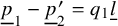 $\underline {p}_1 - \underline {p}_2' = q_1 \underline {l}$
and
 $\underline {p}_2 - \underline {p}_2' = q_2 \underline {l}$
for some (unique)
 $\underline {l} \in \mathbb {Z}^2$
, thus proving (6.2).
Hence, for a fixed choice of
 $(\underline {p}_1',\underline {p}_2') \in E_{\underline {k}}(q_1,q_2)$
, the identity (6.2) allows us to rewrite the term
 $C_{\underline {k}}(q_1,q_2)$
as follows:
 $$ \begin{align*} C_{\underline{k}}(q_1,q_2) &= \sum_{\underline{l}} \int_{[0,1)^2} \chi_{B_1}(\underline{p}_1' + q_1(\underline{l} + \underline{x})) \chi_{B_2}(\underline{p}_2' + q_2(\underline{l} + \underline{x})) \, d\underline{x} \\[0.1cm] &= \int_{\mathbb{R}^2} \chi_{B_1}(\underline{p}_1' + q_1\underline{x}) \chi_{B_2}(\underline{p}_2' + q_2 \underline{x}) \, d\underline{x} \\[0.2cm] &= \int_{\mathbb{R}^2} \chi_{B_1}(\underline{p}_1' - q_1\underline{p}_2'/q_2 + q_1 \underline{x}) \chi_{B_2}(q_2\underline{x}) \, d\underline{x} \\[0.2cm] &= \int_{\mathbb{R}^2} \chi_{B_1}(\underline{k}/q_2 + q_1 \underline{x}) \chi_{B_2}(q_2\underline{x}) \, d\underline{x}, \end{align*} $$
where, in the last step, we have used the fact that
 $q_2 \underline {p}_1' - q_1 \underline {p}_2' = \underline {k}$
. We conclude that
 $$ \begin{align*} C_{\underline{k}}(q_1,q_2) &= \operatorname{\mathrm{Vol}}_2\left( \left(\frac{1}{q_1}B_1 - \frac{\underline{k}}{q_1q_2} \right) \cap \frac{1}{q_2}B_2\right) \\[0.2cm] &= \left( \frac{1}{q_1q_2} \right)^2 \cdot \operatorname{\mathrm{Vol}}_2\left( \left(q_2 B_1 - \underline{k} \right) \cap q_1 B_2 \right). \end{align*} $$
In particular,
 $$ \begin{align*} C_{\underline{k}}(q_1,q_2) &\leq \left( \frac{1}{q_1q_2} \right)^2 \cdot \min\left( \operatorname{\mathrm{Vol}}_2\left(q_2 B_1\right), \operatorname{\mathrm{Vol}}_2\left(q_1 B_2\right)\right) \\[0.2cm] &= \min\left(\frac{\operatorname{\mathrm{Vol}}_2(B_1)}{q_1^2}, \frac{\operatorname{\mathrm{Vol}}_2(B_2)}{q_2^2} \right) \quad \text{for all } \underline{k} \in \mathbb{Z}^2, \end{align*} $$
and
 $$\begin{align*}C_{\underline{k}}(q_1,q_2) = 0, \quad \text{for all } \underline{k} \notin q_2 B_1 - q_1 B_2. \end{align*}$$
Hence,
 $$\begin{align*}\sum_{\underline{k} \in \mathbb{Z}^2} C_{\underline{k}}(q_1,q_2) \leq \left| \mathbb{Z}^2 \cap \left(q_2 B_1 - q_1 B_2\right)\right| \cdot \min\left(\frac{\operatorname{\mathrm{Vol}}_2(B_1)}{q_1^2}, \frac{\operatorname{\mathrm{Vol}}_2(B_2)}{q_2^2} \right), \end{align*}$$
which finishes the proof.
Proof of Lemma 6.1
Fix
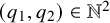 $(q_1,q_2) \in \mathbb {N}^2$
and write
 $q_1 = s q^{\prime }_1$
and
 $q_2 = s q_2'$
, where
 $s = \gcd (q_1,q_2)$
and
 $q_1'$
and
 $q_2'$
are relatively prime. Since multiplication by positive integers on the torus
 $\mathbb {R}^2/\mathbb {Z}^2$
preserves the Lebesgue measure, we have
 $$\begin{align*}\int_{[0,1)^2} N_{D^{(1)}_t}(q_1\underline{x}) N_{D^{(2)}_t}(q_2\underline{x}) \, d\underline{x} = \int_{[0,1)^2} N_{D^{(1)}_t}(q^{\prime}_1\underline{x}) N_{D^{(2)}_t}(q^{\prime}_2\underline{x}) \, d\underline{x}. \end{align*}$$
If we apply Lemma 6.2 to the right-hand side with
 $$\begin{align*}B_1 = D^{(1)}_t \quad \text{and} \quad B_2 = D^{(2)}_t, \end{align*}$$
and note that  , where
 $$\begin{align*}M_i = 2 \max(q_1',q_2') \cdot M \cdot e^{-t_i} \quad \text{for } i = 1,2. \end{align*}$$
we get
 $$ \begin{align*} \int_{[0,1)^2} N_{D^{(1)}_t}(q^{\prime}_1\underline{x}) N_{D^{(2)}_t}(q^{\prime}_2\underline{x}) \, d\underline{x} &\leq \left| \mathbb{Z}^2 \cap \left(q^{\prime}_2 D^{(1)}_t - q^{\prime}_1 D^{(2)}_t\right) \right| \cdot \min\left( \frac{\operatorname{\mathrm{Vol}}_2\left(D^{(1)}_t\right)}{(q^{\prime}_1)^2},\frac{\operatorname{\mathrm{Vol}}_2\left(D^{(2)}_t\right)}{(q^{\prime}_2)^2} \right) \\[0.2cm] &\leq \frac{G(M_1,M_2)}{\max(q^{\prime}_1,q_2')^2} \cdot e^{-(t_1 + t_2)} \cdot \max\left(\operatorname{\mathrm{Vol}}_2\left(D^{(1)}\right),\operatorname{\mathrm{Vol}}_2\left(D^{(2)}\right)\right), \end{align*} $$
where G is defined as in (B.2). Hence,
 $$\begin{align*}\int_{[0,1)^2} N_{D^{(1)}_t}(q^{\prime}_1\underline{x}) N_{D^{(2)}_t}(q^{\prime}_2\underline{x}) \, d\underline{x} \leq F_t(\max(q_1',q_2')) \cdot \max\left(\operatorname{\mathrm{Vol}}_2(D^{(1)}),\operatorname{\mathrm{Vol}}_2(D^{(2)})\right), \end{align*}$$
where
 $F_t$
is defined as in (B.3). This finishes the proof.
7 Mean counting within controlled sets
In this section we prove
 $L^2$
-bounds for Siegel transforms of indicator functions of controlled sets. These bounds will be useful later in Section 8 when we analyze smooth approximations of counting functions.
Lemma 7.1. Let
 $M>1$
and
 $0 < \varepsilon <3\varepsilon < \gamma <1$
. We suppose that
 $E \subset \mathbb {R}^2 \times \mathbb {R}$
is an
 $(\varepsilon ,\gamma ,M)$
-controlled set. Then, for all
 $t = (t_1,t_2) \in \mathbb {R}^2_{+}$
such that
 $$\begin{align*}t_1 + t_2>\max(1,-\ln\left({\gamma}/{2}\right)), \end{align*}$$
we have
 $$\begin{align*}\int_{[0,1)^2} \widehat{\chi}_E(a(t)\Lambda_{\underline{x}})^2 \, d\underline{x} \ll_M e^{-(t_1 + t_2)} + \max\left(\varepsilon,-\frac{\varepsilon}{\gamma} \ln\left(\frac{\varepsilon}{\gamma}\right)\right) \cdot \max(1,(t_1 + t_2))^2, \end{align*}$$
where the implicit constants depend only on M.
Proof. Let
 $E \subset \mathbb {R}^2 \times \mathbb {R}$
be a bounded Borel set, let
 $E(t) = a(t)^{-1}E$
, and note that
 $$ \begin{align*} \int_{[0,1)^2} \widehat{\chi}_E(a(t)\Lambda_{\underline{x}})^2 \, d\underline{x} &\leq \sum_{q_1,q_2 \in \mathbb{Z}} \, \sum_{\underline{p}_1,\underline{p}_2 \in \mathbb{Z}^2} \int_{[0,1)^2} \chi_{E(t)^{q_1}}(\underline{p}_1 + q_1\underline{x}) \chi_{E(t)^{q_2}}(\underline{p}_2 + q_2\underline{x}) \, d\underline{x} \\[0.2cm] &= \sum_{q_1,q_2 \in \mathbb{Z}} \int_{[0,1)^2}N_{D_{q_1}}(q_1 \underline{x}) N_{D_{q_2}}(q_2\underline{x}) \, d\underline{x}, \end{align*} $$
where
 $N_{\bullet }$
is defined as in (6.1) and
 $D_q = E(t)^{q}$
for
 $q \in \mathbb {Z}$
. We define
 $$\begin{align*}J := \{ y \in \mathbb{R} \, : \, E^y \neq \emptyset \}, \end{align*}$$
and note that for every
 $q \in \mathbb {Z}$
,
 $$\begin{align*}E(t)^q = \left( \begin{matrix} e^{-t_1} & \\ & e^{-t_2} \end{matrix} \right)E^{q(t)}, \end{align*}$$
where
 $q(t) = e^{-(t_1 + t_2)}q$
. In particular,
 $$\begin{align*}E(t)^q \neq \emptyset \iff q \in J_t := e^{t_1 + t_2}J. \end{align*}$$
Hence,
 $$\begin{align*}\int_{[0,1)^2} \widehat{\chi}_E(a(t)\Lambda_{\underline{x}})^2 \, d\underline{x} \ll \sum_{q_1,q_2 \in J_t} \int_{[0,1)^2}N_{D^{(1)}_t}(q_1\underline{x}) N_{D^{(2)}_t}(q_2\underline{x}) \, d\underline{x}, \end{align*}$$
where
 $D^{(i)} = E^{q_i(t)}$
for
 $i =1,2$
, and
 $D^{(i)}_t$
is defined as in Lemma 6.1. The same lemma now tells us that
 $$ \begin{align*} \int_{[0,1)^2} \widehat{\chi}_E(a(t)\Lambda_{\underline{x}})^2 \, d\underline{x} &\ll \sum_{q_1,q_2 \in J_t} F_t\left(\frac{\max(q_1,q_2)}{\gcd(q_1,q_2)}\right) \cdot \max\left(\operatorname{\mathrm{Vol}}_{2}\left(E^{q_1(t)}\right),\operatorname{\mathrm{Vol}}_2\left(E^{q_2(t)}\right)\right) \\[0.2cm] &\ll \left(\sum_{q_1,q_2 \in J_t} F_t\left(\frac{\max(q_1,q_2)}{\gcd(q_1,q_2)}\right)\right) \cdot \sup_{y \in J} \operatorname{\mathrm{Vol}}_2(E^y), \end{align*} $$
where
 $F_t$
is defined as in (B.3).
The arguments up to this point have not made use of any special properties of E. In what follows, we will fix
 $0 < \varepsilon < 3\varepsilon < \gamma $
and assume that E is an
 $(\varepsilon ,\gamma ,M)$
-controlled set (see Definition 4.1). The analysis will depend on whether E is type I or type II.
Let us first assume that E is type I. Then,
 $$\begin{align*}J \subset (\gamma,M] \quad \text{and} \quad \sup_{y \in J} \operatorname{\mathrm{Vol}}_2(E^y) \ll_M \max\left(\varepsilon,-\frac{\varepsilon}{\gamma} \ln\left(\frac{\varepsilon}{\gamma}\right)\right). \end{align*}$$
Furthermore, by Lemma B.1 (with
 $\alpha = \gamma $
and
 $\beta = M$
),
 $$\begin{align*}\sum_{q_1,q_2 \in J_t} F_t\left(\frac{\max(q_1,q_2)}{\gcd(q_1,q_2)}\right) \ll_M e^{-(t_1 + t_2)} + \max(1,-\ln(\gamma)) \cdot \max(1,t_1 + t_2), \end{align*}$$
provided that
 $$ \begin{align} t_1 + t_2>\max(1, -\ln(\gamma)). \end{align} $$
We conclude that if the conditions (7.1) hold, then
 $$ \begin{align} \int_{[0,1)^2} \widehat{\chi}_E(a(t)\Lambda_{\underline{x}})^2 \, d\underline{x} \ll (t_1 + t_2)^2 \cdot \max\left(\varepsilon,-\frac{\varepsilon}{\gamma} \ln\left(\frac{\varepsilon}{\gamma}\right)\right). \end{align} $$
Let us now assume that E is type II. Then,
 $$\begin{align*}E \subset [-M,M]^2 \times [\alpha,\beta], \end{align*}$$
where
 $\frac {\gamma }{2} \leq \alpha $
, and
 $\beta - \alpha \ll \varepsilon $
. In particular,
 $$\begin{align*}J \subset [\alpha,\beta] \quad \text{and} \quad \sup_{y \in J} \operatorname{\mathrm{Vol}}_2(E^y) \ll M^2. \end{align*}$$
By Lemma B.1,
 $$ \begin{align*} \sum_{q_1,q_2 \in J_t} F_t\left(\frac{\max(q_1,q_2)}{\gcd(q_1,q_2)}\right) &\ll_M e^{-(t_1+t_2)} + (\beta-\alpha) \cdot \max\left(1,\ln\left(\frac{\beta}{\alpha}\right)\right) \cdot \max(1,t_1 + t_2) \\[0.2cm] &\ll_M e^{-(t_1+t_2)} + \varepsilon \cdot \max\left(1,\ln\left(\frac{\beta}{\alpha}\right)\right) \cdot \max(1,(t_1 + t_2)), \end{align*} $$
provided that
 $$ \begin{align} t_1 + t_2> -\ln(\alpha). \end{align} $$
Note that
 $$\begin{align*}\max\left(1,\ln\left(\frac{\beta}{\alpha}\right)\right) \leq \max\left(1,\frac{\beta-\alpha}{\alpha}\right). \end{align*}$$
If
 $\beta \leq 2\alpha $
, the right-hand side is bounded from above by
 $1$
. Otherwise, the right-hand side is bounded from above by
 $$\begin{align*}\frac{\beta-\alpha}{\alpha} \ll \frac{\varepsilon}{\alpha} \ll \frac{\varepsilon}{\gamma}, \end{align*}$$
since
 $\frac {\gamma }{2} \leq \alpha $
. Hence,
 $$ \begin{align} \int_{[0,1)^2} \widehat{\chi}_E(a(t)\Lambda_{\underline{x}})^2 \, d\underline{x} \ll e^{-(t_1 + t_2)} + \max\left(\varepsilon,\frac{\varepsilon^2}{\gamma}\right) \cdot \max(1,(t_1 + t_2)), \end{align} $$
provided that (7.3) hold.
Now we combine (7.2) and (7.4). Since
 $3\varepsilon < \gamma $
, we have
 $$\begin{align*}\frac{\varepsilon^2}{\gamma} \leq -\frac{\varepsilon}{\gamma} \ln\left(\frac{\varepsilon}{\gamma}\right). \end{align*}$$
Hence, if we combine (7.2) and (7.4), we get the uniform estimate (independent of whether E is type I or type II):
 $$\begin{align*}\int_{[0,1)^2} \widehat{\chi}_E(a(t)\Lambda_{\underline{x}})^2 \, d\underline{x} \ll e^{-(t_1 + t_2)} + \max\left(\varepsilon,-\frac{\varepsilon}{\gamma} \ln\left(\frac{\varepsilon}{\gamma}\right)\right) \cdot \max(1,(t_1 + t_2))^2, \end{align*}$$
provided that (7.1) and (7.3) both hold. Note that since
 $\frac {\gamma }{2} \leq \alpha $
, the second conditions in (7.1) and (7.3) are both satisfied if
 $$\begin{align*}t_1 + t_2> \max(1,-\ln\left({\gamma}/{2}\right)). \end{align*}$$
This finishes the proof.
8 Smooth approximations
Let
 $\mathcal {L}_3$
denote the space of unimodular lattices in
 $\mathbb {R}^3$
. We can identify
 $\mathcal {L}_3$
with the homogeneous space
 $\operatorname {SL}_3(\mathbb {R})/\operatorname {SL}_3(\mathbb {Z})$
via the map
 $g \operatorname {SL}_3(\mathbb {Z}) \mapsto g\mathbb {Z}^3$
. Fix a basis
 $\{Y_1,\ldots ,Y_8\}$
of the Lie algebra
 $\mathfrak {sl}_3(\mathbb {R})$
. We adopt the following slight abuse of notation: for every
 $i = 1,\ldots ,8$
, let
 $D_i$
both denote the differential operator
 $$\begin{align*}D_i \rho(g) = \frac{d}{dt} \rho(\exp(tY_i)g)|_{t=0} \end{align*}$$
on
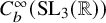 $C_b^\infty (\operatorname {SL}_3(\mathbb {R}))$
and the differential operator
 $$\begin{align*}D_i \varphi = \frac{d}{dt} \rho(\exp(tY_i)\Lambda)|_{t=0} \end{align*}$$
on
 $C_b^\infty (\mathcal {L}_3)$
(which we identify with the space of bounded and smooth right
 $\Gamma $
-invariant functions on the group
 $\operatorname {SL}_3(\mathbb {R})$
via the map above). Differential operators can clearly be composed, and any composition of the
 $D_1,\ldots ,D_8$
can be rewritten as a linear combination of compositions of the form
 $D_m := D_1^{m_1} \circ \cdots \circ D_8^{m_8}$
for some vector
 $m = (m_1,\ldots ,m_8) \in \mathbb {N}_o^8$
(with the convention that
 $D_0 = \operatorname {\mathrm {id}}$
). We define the norms
 $$\begin{align*}\|\rho\|_{C_b^s(\operatorname{SL}_3(\mathbb{R})} := \max\{ \|D_m \rho\|_\infty \, : \, m_1 + \ldots + m_8 \leq s\}, \quad \text{for } \rho \in C_b^\infty(\operatorname{SL}_3(\mathbb{R})) \end{align*}$$
and
 $$\begin{align*}\|\varphi\|_{C^s(\mathcal{L}_3)} := \max\{ \|D_m \varphi\|_\infty \, : \, m_1 + \ldots + m_8 \leq s\}, \quad \text{for } \varphi \in C_b^\infty(\mathcal{L}_3). \end{align*}$$
Fix a right-invariant Riemannian metric on
 $\operatorname {SL}_3(\mathbb {R})$
, and denote by
 $\operatorname {\mathrm {Lip}}$
the corresponding Lipschitz semi-norm on
 $\mathcal {L}_3$
(viewed as the right quotient space
 $\operatorname {SL}_3(\mathbb {R})/\operatorname {SL}_3(\mathbb {Z})$
). We define
 $$ \begin{align} \mathcal{N}_s(\varphi) := \max\big(\|\varphi\|_{C_b^s(\mathcal{L}_3)},\operatorname{\mathrm{Lip}}(\varphi)\big), \quad \text{for } \varphi \in C^\infty(\mathcal{L}_3). \end{align} $$
For
 $\varepsilon> 0$
, let
 $V_\varepsilon $
denote the symmetric open neighborhoods around the identity in
 $\operatorname {SL}_3(\mathbb {R})$
defined in (4.3). For the rest of this paper, we fix a non-negative smooth function
 $\rho _\varepsilon $
on
 $\operatorname {SL}_3(\mathbb {R})$
whose support is contained in
 $V_\varepsilon $
and has integral one with respect to the Haar measure on
 $\operatorname {SL}_3(\mathbb {R})$
. We leave it to the reader to verify that
 $\rho _\varepsilon $
can be chosen so that for every integer
 $s \geq 1$
, there is an integer
 $\sigma _s> 0$
such that
 $$ \begin{align} \|\rho_\varepsilon\|_{C_b^s(\operatorname{SL}_3(\mathbb{R}))} \ll \varepsilon^{-\sigma_s}, \quad \text{for all } \varepsilon\in (0,1) \end{align} $$
and where the implicit constants do not depend on
 $\varepsilon $
.
By Lemma [Reference Björklund and Gorodnik1, Lemma 4.11], for every
 $L> 1$
there exists a smooth function
 $\eta _L : \mathcal {L}_3 \rightarrow [0,1]$
such that
 $$ \begin{align} \{ \operatorname{\mathrm{ht}} \leq L/2 \} \subset \{ \eta_L = 1 \} \subset \operatorname{\mathrm{supp}}(\eta_L) \subset \{ \operatorname{\mathrm{ht}} \leq 2L \}, \end{align} $$
where
 $\operatorname {\mathrm {ht}}$
is the height function on
 $\mathcal {L}_3$
defined in (5.1), with the property that for every
 $s \geq 1$
and
 $m \in \mathbb {N}_o^8$
such that
 $m_1 + \ldots + m_8 \leq s$
, we have
 $$ \begin{align} D_m \eta_L \ll_s 1, \quad \text{for all } L \geq 1, \end{align} $$
where the implicit constants only depend on s, but not on L.
If F is a locally bounded Borel function on
 $\mathbb {R}^3$
and
 $\rho \in C_c^\infty (G)$
, we denote by
 $\rho * F$
the (action) convolution
 $$\begin{align*}(\rho * F)(u) := \int_{G} \rho(g) \, F(g^{-1}u) \, dm(g), \quad \text{for } u \in \mathbb{R}^3, \end{align*}$$
where m is a (fixed) Haar measure on
 $\operatorname {SL}_3(\mathbb {R})$
. We note that
 $$ \begin{align} D_m(\rho * F) := (D_m \rho) * F, \quad \text{for every } m \in \mathbb{N}_o^8. \end{align} $$
Finally, if
 $\varphi $
is a locally bounded function on
 $\mathcal {L}_3$
, we write
 $$\begin{align*}(\rho * \varphi)(u) = \int_{G} \rho(g) \, \varphi(g^{-1}\Lambda) \, dm(g), \quad \text{for } \Lambda \in \mathcal{L}_3. \end{align*}$$
Our first main result in this section now reads as follows.
Lemma 8.1. Let B be a bounded subset of
 $\mathbb {R}^3$
and let
 $s \geq 1$
be an integer. Then, for every bounded Borel function
 $f : \mathbb {R}^3 \rightarrow \mathbb {R}$
such that
 $\{f\neq 0\} \subset B$
and for every
 $L> 1$
and
 $\varepsilon \in (0,1)$
, the Siegel transform
 $\hat {f}$
satisfies
 $$\begin{align*}\mathcal{N}_s((\rho_\varepsilon * \widehat{f}) \cdot \eta_L) \ll_{B,s} \varepsilon^{-\sigma_s} \cdot L \cdot \|f\|_\infty, \end{align*}$$
where the implicit constants only depend on B and s.
8.1 Proof of Lemma 8.1
We first establish pointwise upper bounds on
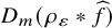 $D_m (\rho _\varepsilon *\widehat {f})$
, for an arbitrary multi-index m.
Lemma 8.2. Let B be a bounded subset of
 $\mathbb {R}^3$
and let
 $s \geq 1$
be an integer. Then, for every
 $0 < \varepsilon < 1$
,
 $L> 1$
and for every bounded Borel function
 $f : \mathbb {R}^3 \rightarrow \mathbb {R}$
such that
 $\{f\neq 0\} \subset B$
and for every multi-index
 $m = (m_1,\ldots ,m_8) \in \mathbb {N}_o^8$
such that
 $m_1 + \ldots + m_8 \leq s$
, we have
 $$\begin{align*}|D_m ((\rho_\varepsilon *\widehat{f})\cdot \eta_L)| \ll_{B,s} \varepsilon^{-\sigma_s} \cdot \|f\|_\infty \cdot L, \quad \text{for all } \Lambda \in \mathcal{L}_3, \end{align*}$$
where the implicit constants only depend on B and s.
Proof. Note that

Hence, by Lemma 5.2,
 $$\begin{align*}|(D_m(\rho_\varepsilon * \widehat{f})(\Lambda)| \ll_B \|D_m(\rho_\varepsilon) * f\|_\infty \cdot \operatorname{\mathrm{ht}}(\Lambda) \ll \|\rho_\varepsilon\|_{C^s(\operatorname{SL}_3(\mathbb{R}))} \cdot \|f\|_\infty \cdot \operatorname{\mathrm{ht}}(\Lambda), \end{align*}$$
for every
 $\Lambda \in \mathcal {L}_3$
and
 $m = (m_1,\ldots ,m_8)$
such that
 $m_1 + \ldots m_8 \leq s$
, where the implicit constants only depend on the support of
 $D_m(\rho _\varepsilon ) * f$
, which is contained in
 $V_\varepsilon. B$
(and thus in a ball of radius
 $2R$
, where R is the smallest radius of a ball enclosing B). By (8.2),
 $\|\rho _\varepsilon \|_{C_b^s(\operatorname {SL}_3(\mathbb {R}))} \ll \varepsilon ^{-\sigma _s}$
, and we obtain the bound
 $$\begin{align*}|D_m (\rho_\varepsilon *\widehat{f})(\Lambda)| \ll_{B,s} \varepsilon^{-\sigma_s} \cdot \|f\|_\infty \cdot \text{ht}(\Lambda), \quad \text{for all } \Lambda \in \mathcal{L}_3, \end{align*}$$
Now the lemma follows from (8.4).
Let us now discuss Lipschitz semi-norms. By definition, if
 $\Lambda \in \mathcal {L}_3$
and
 $\operatorname {\mathrm {dist}}$
is a right-invariant distance on
 $\operatorname {SL}_3(\mathbb {R})$
, we can induce a (noninvariant) distance on
 $\mathcal {L}_3$
by
 $$\begin{align*}\operatorname{\mathrm{dist}}(\Lambda,h.\Lambda) = \inf \left\{ \operatorname{\mathrm{dist}}(\operatorname{\mathrm{id}},h\gamma) \, : \, \gamma \in \operatorname{\mathrm{Stab}}_{\operatorname{SL}_3(\mathbb{R})}(\Lambda) \right\}, \quad \text{for } h \in \operatorname{SL}_3(\mathbb{R}). \end{align*}$$
The corresponding Lipschitz semi-norms on
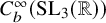 $C_b^\infty (\operatorname {SL}_3(\mathbb {R}))$
and
 $C_b^\infty (\mathcal {L}_3)$
are thus given by
 $$\begin{align*}\operatorname{\mathrm{Lip}}_{\operatorname{SL}_3(\mathbb{R})}(\rho) = \sup\left\{ \frac{|\rho(g) - \rho(hg)|}{\operatorname{\mathrm{dist}}(\operatorname{\mathrm{id}},h)} \, : \, g,h \in \operatorname{SL}_3(\mathbb{R}), h \neq \operatorname{\mathrm{id}} \right\}, \end{align*}$$
for
 $\rho \in C_b^\infty (\operatorname {SL}_3(\mathbb {R}))$
and
 $$\begin{align*}\operatorname{\mathrm{Lip}}_{\mathcal{L}_3}(\varphi) = \sup\left\{ \frac{|\varphi(\Lambda) - \varphi(h.\Lambda)|}{\operatorname{\mathrm{dist}}(\Lambda,h.\Lambda)} \, : \, \Lambda \in \mathcal{L}_3, h \notin \operatorname{\mathrm{Stab}}_{\operatorname{SL}_3(\mathbb{R})}(\Lambda) \right\}, \end{align*}$$
for
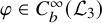 $\varphi \in C_b^\infty (\mathcal {L}_3)$
.
One checks that there is a constant
 $\theta> 0$
such that
 $$ \begin{align} \operatorname{\mathrm{Lip}}_{\operatorname{SL}_3(\mathbb{R})}(\rho_\varepsilon) \ll \varepsilon^{-\theta}, \end{align} $$
with implicit constants that are independent of
 $\varepsilon $
. Upon possibly enlarging
 $\sigma _s$
, we can (and will) always assume that
 $\theta < \sigma _s$
. We also leave to the reader to show that the function
 $\eta _{L}$
can be chosen so that
 $$ \begin{align} \left|\eta_L(\Lambda)-\eta_L(h.\Lambda)\right| \ll \operatorname{\mathrm{dist}}(\Lambda,h.\Lambda), \end{align} $$
with implicit constants that are independent of L.
Lemma 8.3. Let B be a bounded subset of
 $\mathbb {R}^3$
. Then, for every
 $0 < \varepsilon < 1$
and for every bounded Borel function
 $f : \mathbb {R}^3 \rightarrow \mathbb {R}$
such that
 $\{f\neq 0\} \subset B$
and
 $L \geq 1$
,
 $$\begin{align*}\operatorname{\mathrm{Lip}}_{\mathcal{L}_3}((\rho_\varepsilon * \widehat{f}) \cdot \eta_L) \ll_B \varepsilon^{-\theta} \cdot L, \end{align*}$$
where the implicit constants only depend on B.
Proof. We use in the proof that
 $$ \begin{align*}\|\rho_\varepsilon\|_{C_b^s(\operatorname{SL}_3(\mathbb{R}))}\ll \varepsilon^{-\theta}\quad \text{and} \quad \operatorname{\mathrm{Lip}}_{\operatorname{SL}_3(\mathbb{R})}(\rho_\varepsilon) \ll \varepsilon^{-\theta}. \end{align*} $$
For every
 $h \in G$
and
 $\Lambda \in \mathcal {L}_3$
, we have
 $$ \begin{align*} \left| (\rho_\varepsilon * \widehat{f})(\Lambda) - (\rho_\varepsilon * \widehat{f})(h.\Lambda)\right| &\leq \int_{(V_\varepsilon \cup h^{-1}V_\varepsilon)} \left|\rho_\varepsilon(g) - \rho_\varepsilon(hg)\right| \cdot \widehat{f}(g^{-1}.\Lambda) \, dg \\[0.2cm] &\leq \operatorname{\mathrm{Lip}}_{\operatorname{SL}_3(\mathbb{R})}(\rho_\varepsilon) \cdot \operatorname{\mathrm{dist}}(\operatorname{\mathrm{id}},h) \cdot \int_{(V_\varepsilon \cup h^{-1}V_\varepsilon)} |\widehat{f}(g^{-1}.\Lambda)| \, dm(g) \\[0.2cm] &\ll \varepsilon^{-\theta} \cdot \operatorname{\mathrm{dist}}(\operatorname{\mathrm{id}},h) \cdot \int_{(V_\varepsilon \cup h^{-1}V_\varepsilon)} |\widehat{f}(g^{-1}.\Lambda)| \, dm(g), \end{align*} $$
where we in the last estimate have used (8.6). Note that the same computation goes through with
 $h_\gamma := h\gamma $
for
 $\gamma \in \operatorname {\mathrm {Stab}}_{\operatorname {SL}_3(\mathbb {R})}(\Lambda )$
, and thus
 $$ \begin{align} \left| (\rho_\varepsilon * \widehat{f})(\Lambda) - (\rho_\varepsilon * \widehat{f})(h.\Lambda)\right| \leq \varepsilon^{-\theta} \cdot \operatorname{\mathrm{dist}}(\Lambda,h.\Lambda) \cdot \int_{(V_\varepsilon \cup h_\gamma^{-1}V_\varepsilon)} |\widehat{f}(g^{-1}.\Lambda)| \, dm(g). \end{align} $$
We also note that
 $$ \begin{align} ((\rho_\varepsilon * \widehat{f}) \cdot \eta_L)(\Lambda) - ((\rho_\varepsilon * \widehat{f}) \cdot \eta_L)(h.\Lambda) =\ & \left((\rho_\varepsilon * \widehat{f})(\Lambda) -(\rho_\varepsilon * \widehat{f})(h.\Lambda)\right) \cdot \eta_L(\Lambda) \nonumber \\[0.2cm] &+ (\rho_\varepsilon * \widehat{f})(h.\Lambda) \cdot \left(\eta_L(\Lambda)-\eta_L(h.\Lambda)\right). \end{align} $$
We can without loss of generality assume that at least one of the points
 $\Lambda $
and
 $h.\Lambda $
belong to
 $\operatorname {\mathrm {supp}}(\eta _L)$
; otherwise the Lipschitz condition is trivially satisfied. The rest of our analysis is now divided into two cases.
Case I:
$\Lambda , h.\Lambda \in \operatorname {\mathrm {supp}}(\eta _L)$
, so that
$\mathrm {ht}(\Lambda ), \mathrm {ht}(h\Lambda )\le 2L$


By Lemma 5.2 and (5.2), we have
 $$\begin{align*}|\widehat{f}(g^{-1}h.\Lambda)| \ll_{B} \|f\|_\infty \cdot \operatorname{\mathrm{ht}}(g^{-1}h.\Lambda) \leq \|f\|_\infty \cdot \|g\|_{\text{op}} \cdot \operatorname{\mathrm{ht}}(h.\Lambda) , \quad \text{for all } g,h \in \operatorname{SL}_3(\mathbb{R}), \end{align*}$$
and thus,
 $$ \begin{align} \int_{(V_\varepsilon \cup h_\gamma^{-1}V_\varepsilon)} |\widehat{f}(g^{-1}.\Lambda)| \, dg &\leq \int_{V_\varepsilon} |\widehat{f}(g^{-1}.\Lambda)| \, dg + \int_{V_\varepsilon} |\widehat{f}(g^{-1}h.\Lambda)| \, dg\nonumber \\[0.2cm] &\ll_B (1+\varepsilon) \cdot \|f\|_\infty \cdot \operatorname{\mathrm{ht}}(\Lambda) + (1+\varepsilon) \cdot \operatorname{\mathrm{ht}}(h.\Lambda)\nonumber \\[0.2cm] &\ll \|f\|_\infty \cdot \max(\operatorname{\mathrm{ht}}(\Lambda),\operatorname{\mathrm{ht}}(h.\Lambda)), \end{align} $$
for all
 $g \in V_\varepsilon $
and for all
 $h \in \operatorname {SL}_3(\mathbb {R})$
, where the implicit constants only depend on B (and not on
 $\varepsilon \in (0,1)$
). Hence, we deduce from (8.8) and (8.10) that the first term on the right-hand side in (8.9) is bounded above in absolute value by
 $$ \begin{align} \ll \|f\|_\infty \cdot \max(\operatorname{\mathrm{ht}}(\Lambda),\operatorname{\mathrm{ht}}(h.\Lambda)) \cdot \eta_L(\Lambda) \cdot \operatorname{\mathrm{dist}}(\Lambda,h.\Lambda) \cdot \varepsilon^{-\theta}, \end{align} $$
while the second term is bounded above in absolute value by
 $$ \begin{align} \ll \|f\|_\infty \cdot \operatorname{\mathrm{ht}}(h.\Lambda) \cdot \left|\eta_L(\Lambda)-\eta_L(h.\Lambda)\right| \ll \|f\|_\infty \cdot \operatorname{\mathrm{ht}}(h.\Lambda) \cdot \varepsilon^{-\theta} \cdot \operatorname{\mathrm{dist}}(\Lambda,h.\Lambda), \end{align} $$
where we in the last inequality have used (8.7). By our assumption,
 $\operatorname {\mathrm {ht}}(\Lambda ) \leq 2L$
and
 $\operatorname {\mathrm {ht}}(h.\Lambda ) \leq 2L$
, so we conclude that
 $$\begin{align*}\left| (\rho_\varepsilon * \widehat{f})(\Lambda) - (\rho_\varepsilon * \widehat{f})(h.\Lambda)\right| \ll \|f\|_\infty \cdot \varepsilon^{-\theta} \cdot L \cdot \operatorname{\mathrm{dist}}(\Lambda,h.\Lambda). \end{align*}$$
Case II:
$\Lambda \in \operatorname {\mathrm {supp}}(\eta _L)$
but
$h.\Lambda \notin \operatorname {\mathrm {supp}}(\eta _L)$
or the opposite


We split this case into two subcases. Let us first assume that
 $\operatorname {\mathrm {dist}}(\Lambda ,h.\Lambda ) \geq 1$
. Then, by the same analysis as above,
 $$ \begin{align*} |(\rho_\varepsilon * \widehat{f})(\Lambda) \eta_L(\Lambda)| &\ll \varepsilon^{-\theta} \cdot \int_{V_\varepsilon} |\widehat{f}(g^{-1}.\Lambda)| \, dm(g) \\[0.2cm] &\ll_B \varepsilon^{-\theta} \cdot \|f\|_\infty \cdot \operatorname{\mathrm{ht}}(\Lambda) \leq \varepsilon^{-\theta} \cdot \|f\|_\infty \cdot L \\[0.2cm] &\ll \varepsilon^{-\theta} \cdot \|f\|_\infty \cdot L \cdot \operatorname{\mathrm{dist}}(\Lambda,h.\Lambda). \end{align*} $$
If
 $\operatorname {\mathrm {dist}}(\Lambda ,h.\Lambda ) \leq 1$
, we can choose
 $h_\gamma $
such that
 $\operatorname {\mathrm {dist}}(\operatorname {\mathrm {id}},h_\gamma ) \leq 1$
, and hence there is a compact set K, which is independent of
 $\varepsilon $
(and h as long as
 $\operatorname {\mathrm {dist}}(\Lambda ,h.\Lambda ) \leq 1$
), with the property that
 $$\begin{align*}V_\varepsilon \cup h_\gamma^{-1}V_\varepsilon \subset K. \end{align*}$$
Hence, in this case, by (8.6), Lemma 5.2 and (5.2),
 $$\begin{align*}\left| (\rho_\varepsilon * \widehat{f})(\Lambda) - (\rho_\varepsilon * \widehat{f})(h.\Lambda)\right| \ll_B \varepsilon^{-\theta} \cdot \operatorname{\mathrm{dist}}(\Lambda,h.\Lambda) \cdot \|f\|_\infty \cdot \left( \int_{K} \|g^{-1}\|_{\text{op}} \, dm(g) \right) \cdot \operatorname{\mathrm{ht}}(\Lambda). \end{align*}$$
Similarly, when
 $\operatorname {\mathrm {dist}}(\Lambda ,h.\Lambda ) \leq 1$
,
 $$\begin{align*}|(\rho_\varepsilon * \widehat{f})(h.\Lambda) | \ll_K \varepsilon^{-\theta} \cdot \|f\|_\infty \cdot \operatorname{\mathrm{ht}}(\Lambda). \end{align*}$$
We conclude that in the difference (8.9) both terms are bounded above in absolute value by
 $$\begin{align*}\ll \|f\|_\infty \cdot \varepsilon^{-\theta} \cdot L \cdot \operatorname{\mathrm{dist}}(\Lambda,h.\Lambda), \end{align*}$$
where we for the second term have used (8.7). In both subcases, we see that
 $$\begin{align*}\left| (\rho_\varepsilon * \widehat{f})(\Lambda) \eta_L(\Lambda) - (\rho_\varepsilon * \widehat{f})(h.\Lambda) \eta_L(h.\Lambda) \right| \ll \|f\|_\infty \cdot \varepsilon^{-\theta} \cdot L \cdot \operatorname{\mathrm{dist}}(\Lambda,h.\Lambda). \end{align*}$$
The opposite case is handled in the same way by interchanging
 $\Lambda $
and
 $h.\Lambda $
, and we are done.
The proof of Lemma 8.1 follows upon combining Lemma 8.2 and Lemma 8.3.
8.2 Smooth approximations of counting functions
In this subsection we discuss smooth approximation of the counting functions that come out of our tessellation scheme in Section 3. We begin by recalling the notation. We have
 $$ \begin{align} \alpha_\Omega = \ln\left(\frac{T_0c^2}{b e^2} \right), \quad \beta_\Omega = \ln\left(\frac{Tc^2}{a}\right), \end{align} $$
and
 $$\begin{align*}\mathcal{F}_\Omega = \left\{ n \in \mathbb{N}_o^2 \, : \, \alpha_\Omega \leq n_1 + n_2 < \beta_\Omega \right\}. \end{align*}$$
We also assume that
 $$ \begin{align} \zeta\cdot b\le c^2\quad \text{and} \quad c<1/2 \end{align} $$
for some
 $\zeta>0$
. Without loss of generality,
 $\zeta <1$
.
For
 $n \in \mathcal {F}_\Omega $
and a bounded measurable function
 $h : [0,\infty ) \rightarrow \mathbb {R}$
, we define
 $$\begin{align*}h_{\Omega,n}(\underline{u},y) := h\left(\frac{e^{n_1 + n_2} \cdot y}{T}\right) \, \chi_{\Delta_{\Omega,n}}(\underline{u},y), \quad \text{for } (\underline{u},y) \in \mathbb{R}^2 \times \mathbb{R}, \end{align*}$$
where
 $\Delta _{\Omega ,n}$
is defined in (3.3). By Lemma 3.1,

Let
 $$\begin{align*}\phi_{\Omega,n} := \widehat{h}_{\Omega,n} - \int_{\mathcal{L}_3} \widehat{h}_{\Omega,n} d\mu, \end{align*}$$
where
 $\mu $
is the unique
 $\operatorname {SL}_3(\mathbb {R})$
-invariant probability measure on
 $\mathcal {L}_3$
.
Let
 $\varepsilon _T$
be a decreasing function, which converges to zero as
 $T \rightarrow \infty $
, and let
 $\rho _{\varepsilon _T}$
be as in the previous subsection (with
 $\varepsilon = \varepsilon _T$
). Let
 $L_T$
be an increasing function, which tends to infinity with T, and define
 $$\begin{align*}f_{\Omega,n}(\underline{u},y) := (\rho_{\varepsilon_T} * h_{\Omega,n})(\underline{u},y), \quad \text{for } (\underline{u},y) \in \mathbb{R}^2 \times \mathbb{R}, \end{align*}$$
and
 $$ \begin{align} \varphi_{\Omega,n} := \widehat{f}_{\Omega,n} \cdot \eta_{L_T} - \int_{\mathcal{L}_3} \widehat{f}_{\Omega,n} \cdot \eta_{L_T} \, d\mu. \end{align} $$
It follows from (8.15) that
 $$ \begin{align} \{ f_{\Omega,n} \neq 0 \} \subset [-1,1]^2 \times [-1,e^2\zeta^{-1}+1] \end{align} $$
for all n and for all sufficiently large T, so that by Theorem 5.1,
 $$ \begin{align} \int_{\mathcal{L}_3} \widehat{f}_{\Omega,n} \cdot \eta_L \, d\mu \leq \int_{\mathcal{L}_3} \widehat{f}_{\Omega,n} \, d\mu = \int_{\mathbb{R}^2 \times \mathbb{R}} f_{\Omega,n}(\underline{u},y) \, d\underline{u} dy\ll_\zeta 1, \end{align} $$
with implicit constants that are independent of T,
 $\varepsilon _T$
and n. Then, (8.16), (8.17), (8.18), and Lemma 8.1 immediately imply the following result.
Lemma 8.4. For every
 $s \geq 1$
and for all sufficiently large T,
 $$\begin{align*}\sup_{n \in \mathcal{F}_\Omega} \mathcal{N}_s(\varphi_{\Omega,n}) \ll_s \varepsilon_T^{-\sigma_s} \cdot L_T, \end{align*}$$
where the implicit constants only depend on
 $\|h\|_\infty $
and s, and not on T.
Let us now assume that h is a bounded Lipschitz continuous function on
 $[0,\infty )$
. The rest of this section is devoted to the proof of the following lemma which roughly asserts that the smooth approximations of
 $\widehat {h}_{\Omega ,n}$
above are good in the
 $L^2(\nu )$
-sense along a-orbits, where
 $\nu $
is the unique
 $\mathbb {R}^2$
-invariant measure on the torus
 $\mathcal {Y}_3 := \{ \Lambda _{\underline {x}} \, : \, \underline {x} \in [0,1)^2 \} \subset \mathcal {L}_3$
.
Lemma 8.5. Suppose that
 $$ \begin{align*}\varepsilon_T < a \zeta^2/100\quad \text{and} \quad L_T \geq 2e^{2}\zeta^{-1}. \end{align*} $$
Then, for all
 $n \in \mathbb {N}^2$
such that
 $n_1+n_2> \max (1,-\ln \left ({a}/{2}\right ))$
, we have
 $$ \begin{align*} \big\|(\phi_{\Omega,n} - \varphi_{\Omega,n}) \circ a(n) \big\|_{L^2(\nu)} &\ll_{h,\zeta} \frac{\varepsilon_T}{a} \cdot \max(1,n_1 + n_2)^{1/2} + e^{-\frac{(n_1 + n_2)}{2}}\\[0.2cm] &\quad + \max\Big(\varepsilon_T,-\frac{\varepsilon_T}{a} \ln\Big(\frac{\varepsilon_T}{a} \Big)\Big)^{1/2} \cdot \max(1,(n_1 + n_2)) \\[0.2cm] &\quad + \left(L_T^{-1/2} + e^{-\frac{\lfloor n \rfloor}{2}} \right)\cdot \max(1,n_1 + n_2)^{1/2}. \end{align*} $$
Remark 8.6. The implicit function in the lemma depends only on
 $\|h\|_\infty $
and
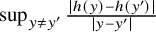 $\sup _{y\neq y'} \frac {|h(y)-h(y')|}{|y-y'|}$
.
Proof. We observe that
 $$ \begin{align} \big\|(\phi_{\Omega,n} - \varphi_{\Omega,n}) \circ a(n) \big\|_{L^2(\nu)} \le \big\| (\widehat{h}_{\Omega,n} - \widehat{f}_{\Omega,n} \cdot \eta_{L_T}) \circ a(n) \big\|_{L^2(\nu)}+\big\| \widehat{h}_{\Omega,n} - \widehat{f}_{\Omega,n} \cdot \eta_{L_T} \big\|_{L^1(\mu)}, \end{align} $$
and
 $$ \begin{align} (\widehat{h}_{\Omega,n} - \widehat{f}_{\Omega,n} \cdot \eta_{L_T}) \circ a(n) = (\widehat{h}_{\Omega,n} - \widehat{f}_{\Omega,n}) \circ a(n) + \left(\widehat{f}_{\Omega,n} \cdot (1-\eta_{L_T})\right) \circ a(n). \end{align} $$
We estimate each of the the above terms separately.
First, we proceed with the estimate of
 $\big \|(\widehat {h}_{\Omega ,n} - \widehat {f}_{\Omega ,n}) \circ a(n)\big \|_{L^2(\nu )}$
. We recall that
 $$ \begin{align*}h_{\Omega,n}(\underline{x},y)=h\left(\frac{e^{n_1 + n_2} \cdot y}{T}\right) \cdot \chi_{\Delta_{\Omega,n}}(\underline{x},y),\quad (\underline{x},y)\in \mathbb{R}^2\times \mathbb{R}. \end{align*} $$
For
 $g \in V_{\varepsilon _T}$
, we write
 $g.(\underline {x},y) := (\underline {x}(g),y(g))$
as in (4.5). Then
 $$ \begin{align*}h_{\Omega,n}(g.(\underline{x},y))=h\left(\frac{e^{n_1 + n_2} \cdot y(g)}{T}\right) \cdot \chi_{\Delta_{\Omega,n}}(\underline{x}(g),y(g)),\quad (\underline{x},y)\in \mathbb{R}^2\times \mathbb{R}. \end{align*} $$
It follows from (8.15) that
 $$\begin{align*}\max(\|\underline{x}-\underline{x}(g)\|_\infty,|y-y(g)|) \ll_\zeta \varepsilon_T, \quad \text{for all } g \in V_{\varepsilon_T} \end{align*}$$
provided that either
 $(\underline {x},y) \in \Delta _{\Omega ,n}$
or
 $(\underline {x}(g),y(g)) \in \Delta _{\Omega ,n}$
, which we assume from now on.
We observe that
 $|h_{\Omega ,n}-h_{\Omega ,n}\circ g|$
can be bounded by
 $$\begin{align*}\left| h\left(\frac{e^{n_1 + n_2} \cdot y}{T}\right) - h\left(\frac{e^{n_1 + n_2} \cdot y(g)}{T}\right)\right| \cdot \chi_{\Delta_{\Omega,n}}(\underline{x},y) + \left|h\left(\frac{e^{n_1 + n_2} y(g)}{T}\right)\right| \cdot \chi_{E_{\Omega,n}(g)}, \end{align*}$$
where
 $$\begin{align*}E_{\Omega,n}(g) := \left(g^{-1}\Delta_{\Omega,n} \setminus \Delta_{\Omega,n}\right) \cup \left(\Delta_{\Omega,n} \setminus g^{-1}\Delta_{\Omega,n}\right). \end{align*}$$
Recall that
 $\Delta _{\Omega ,n}= \emptyset $
unless
 $n\in \mathcal {F}_\Omega $
so that we may assume that
 $n\in \mathcal {F}_\Omega $
, thus
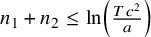 $n_1 + n_2 \leq \ln \left (\frac {Tc^2}{a}\right )$
. Since h is Lipschitz continuous, for
 $n \in \mathcal {F}_\Omega $
, we have
 $$ \begin{align*} \left| h\left(\frac{e^{n_1 + n_2} \cdot y}{T}\right) - h\left(\frac{e^{n_1 + n_2} \cdot y(g)}{T}\right)\right| &\leq \frac{e^{n_1+n_2}}{T} \cdot |y-y(g)| \cdot \operatorname{\mathrm{Lip}}(h), \nonumber \\ &\ll_\zeta \frac{c^2 \cdot \varepsilon_T}{a} \cdot \operatorname{\mathrm{Lip}}(h)\le \frac{\varepsilon_T}{a} \cdot \operatorname{\mathrm{Lip}}(h). \end{align*} $$
We note that the set
 $\Delta _{\Omega ,n}$
is of the form (4.2), with
 $$\begin{align*}a = a, b = b, u_{i}^{-} = e^{-1}c , u_{i}^{+} = c,\text{ for } i=1,2, \end{align*}$$
and with
 $\gamma = \gamma _{\Omega ,n}=T_0e^{-(n_1+n_2)}$
and
 $\delta = \delta _{\Omega ,n}=Te^{-(n_1+n_2)}$
, which, by (8.15) satisfy the bounds
 $$\begin{align*}2a<\frac{a}{c^2} < \gamma_{\Omega,n} \quad \text{and} \quad \delta_{\Omega,n} < \frac{b e^2}{c^2}\le e^2\zeta^{-1} \end{align*}$$
Hence, by Lemma 4.3 (see also Remark 4.2) and the fact that
 $\varepsilon _{T}\leq a_{T}\zeta ^{2}/100$
, we can find
 $(\varepsilon _T,a,e^2\zeta ^{-1}+1)$
-controlled sets
 $E_{\Omega ,n}^{(s)}$
,
 $s=1,\ldots ,24$
, such that
 $$\begin{align*}{E_{\Omega,n}(g)} \subset \bigcup_s {E_{\Omega,n}^{(s)}}, \quad \text{for all } g \in V_{\varepsilon_T}. \end{align*}$$
Therefore, we conclude that for all
 $g\in V_\varepsilon $
and
 $n\in \mathcal {F}_\Omega $
,
 $$\begin{align*}|h_{\Omega,n}(\underline{x},y) - h_{\Omega,n}(g.(\underline{x},y))| \ll_\zeta \left(\frac{ \varepsilon_T}{a} \cdot \chi_{\Delta_{\Omega,n}}(\underline{x},y) + \sum_s \chi_{E_{\Omega,n}^{(s)}}(\underline{x},y)\right) \cdot \operatorname{\mathrm{Lip}}(h), \end{align*}$$
provided that either
 $(\underline {x},y) \in \Delta _{\Omega ,n}$
or
 $(\underline {x}(g),y(g)) \in \Delta _{\Omega ,n}$
. In fact, this estimate holds for all
 $(\underline {x},y)\in \mathbb {R}^2\times \mathbb {R}$
since it holds trivially in the complementary set. Since
 $f_{\Omega ,n}=\rho _{\varepsilon _T}*h_{\Omega ,n}$
, we obtain that
 $$\begin{align*}|h_{\Omega,n} - f_{\Omega,n}| \ll_\zeta \left(\frac{\varepsilon_T}{a} \cdot \chi_{\Delta_{\Omega,n}} + \sum_s \chi_{E_{\Omega,n}^{(s)}}\right) \cdot \operatorname{\mathrm{Lip}}(h). \end{align*}$$
for all
 $n\in \mathbb {N}^2_o$
. We also have the corresponding bounds for the Siegel transforms:
 $$ \begin{align} |\widehat h_{\Omega,n} - \widehat f_{\Omega,n}| \ll_\zeta \left(\frac{\varepsilon_T}{a} \cdot \widehat \chi_{\Delta_{\Omega,n}} + \sum_s \widehat \chi_{E_{\Omega,n}^{(s)}}\right) \cdot \operatorname{\mathrm{Lip}}(h). \end{align} $$
Therefore,
 $$ \begin{align} \big\|(\widehat h_{\Omega,n} - \widehat f_{\Omega,n})\circ a(n)\big\|_{L^2(\nu)} \ll_\zeta & \Big( \frac{\varepsilon_T}{a} \cdot \big\|\widehat{\chi}_{\Delta_{\Omega,n}} \circ a(n)\big\|_{L^2(\nu)} + \sum _s \big\|\widehat{\chi}_{E_{\Omega,n}^{(s)}} \circ a(n)\big\|_{L^2(\nu)}\Big) \cdot \operatorname{\mathrm{Lip}}(h). \end{align} $$
It follows from (8.15) and Lemma 5.2 that
 $$\begin{align*}\big\|\widehat{\chi}_{\Delta_{\Omega,n}} \circ a(n)\big\|_{L^2(\nu)} \ll_\zeta \left( \int_{[0,1)^2} \operatorname{\mathrm{ht}}(a(n)\Lambda_{\underline{x}})^2 \, d\underline{x} \right)^{1/2}, \end{align*}$$
where the implicit constants are independent of
 $\Omega $
and n. Furthermore, Corollary 5.5, applied with
 $\theta (u) = u^2$
and
 $\eta = e^2\zeta ^{-1}$
, tells us that
 $$\begin{align*}\int_{[0,1)^2} \operatorname{\mathrm{ht}}(a(n)\Lambda_{\underline{x}})^2 \, d\underline{x} \ll_\zeta \max(1,n_1+n_2), \end{align*}$$
We conclude that
 $$ \begin{align} \big\|\widehat{\chi}_{\Delta_{\Omega,n}} \circ a(n)\big\|_{L^2(\nu)} \ll \max(1,n_1 + n_2)^{1/2}, \end{align} $$
for all
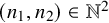 $(n_1,n_2) \in \mathbb {N}^2$
.
Next we estimate
 $\|\widehat {\chi }_{E_{\Omega ,n}^{(s)}} \circ a(n)\|_{L^2(\nu )}$
. Since the sets
 $E_{\Omega ,n}^{(s)}$
are
 $(\varepsilon _T,a,e^2\zeta ^{-1}+1)$
-controlled, it follows from Lemma 7.1 that
 $$ \begin{align} \big\|\widehat{\chi}_{E_{\Omega,n}^{(s)}} \circ a(n)\big\|_{L^2(\nu)} &\ll_\zeta \left( e^{-(n_1 + n_2)} + \max\left(\varepsilon_T,-\frac{\varepsilon_T}{a} \ln\left(\frac{\varepsilon_T}{a}\right)\right) \cdot \max(1,n_1 + n_2)^2 \right)^{1/2}\nonumber \\ &\ll e^{-\frac{(n_1 + n_2)}{2}} + \max\Big(\varepsilon_T,-\frac{\varepsilon_T}{a} \ln\Big(\frac{\varepsilon_T}{a} \Big)\Big)^{1/2} \max(1,n_1 + n_2), \end{align} $$
where the implicit constants are independent of n and T, provided that
 $$ \begin{align} n_1 + n_2> \max(1,-\ln\left(a/2\right)). \end{align} $$
If we now combine (8.23) and (8.24), we get from (8.22)
 $$ \begin{align} \big\|(\widehat h_{\Omega,n} - \widehat f_{\Omega,n})\circ a(n)\big\|_{L^2(\nu)} \ll_{\zeta,h}& \frac{\varepsilon_T}{a} \cdot \max(1,n_1 + n_2)^{1/2} + e^{-\frac{(n_1 + n_2)}{2}}\nonumber\\[0.2cm] &+ \max\Big(\varepsilon_T,-\frac{\varepsilon_T}{a} \ln\Big(\frac{\varepsilon_T}{a} \Big)\Big)^{1/2} \cdot \max(1,(n_1 + n_2)), \end{align} $$
for all
 $n\in \mathbb {N}_o^2$
satisfying (8.25). This provides an estimate of the first term in (8.20).
Now we estimate the term
 $\left \|\left (\widehat {f}_{\Omega ,n} \cdot (1-\eta _{L_T})\right ) \circ a(n) \right \|_{L^2(\nu )}$
. It follows from (8.17) and Lemma 5.2 that
 $$ \begin{align} f_{\Omega,n}\ll_{h,\zeta} \text{ht}. \end{align} $$
Furthermore,
 $$ \begin{align} \operatorname{\mathrm{supp}}(1-\eta_{L_T}) \subset \left\{ \operatorname{\mathrm{ht}} \geq \frac{L_T}{2} \right\}. \end{align} $$
Thus,
 $$\begin{align*}\left\|\left(\widehat{f}_{\Omega,n} \cdot (1-\eta_{L_T})\right) \circ a(n) \right\|_{L^2(\nu)} \ll \left(\int_{M_{T,n}} (\operatorname{\mathrm{ht}}(a(n)\Lambda_{\underline{x}}))^2 \, d\underline{x} \right)^{1/2}, \end{align*}$$
where
 $$\begin{align*}M_{T,n} := \left\{ \underline{x} \in [0,1)^2 \, : \, \operatorname{\mathrm{ht}}(a(n)\Lambda_{\underline{x}}) \geq \frac{L_T}{2}\right\}. \end{align*}$$
Note that
 $M_{T,n} = M_{n,1}(L_T/2)$
, where the latter set is defined as in (5.4). Hence, by Corollary 5.5, applied with
 $\theta (u) = u^2$
, we get
 $$ \begin{align*} \int_{M_{T,n}} (\operatorname{\mathrm{ht}}(a(n)\Lambda_{\underline{x}}))^2 \, d\underline{x} &\ll_\zeta \left(L_T^{-1} + e^{-\lfloor n \rfloor} \right) \cdot \int_{L_T e^{-2}/2}^{e^{n_1 + n_2 + 1}\max(1,\zeta^{-1})} \frac{du}{u} \\ &\ll_\zeta \left(L_T^{-1} + e^{-\lfloor n \rfloor} \right) \cdot \max(1,n_1 + n_2), \end{align*} $$
for all
 $n \in \mathbb {N}_o^2$
, provided that
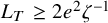 $L_T \geq 2e^{2}\zeta ^{-1}$
. Hence, we conclude that
 $$ \begin{align} \left\|\left(\widehat{f}_{\Omega,n} \cdot (1-\eta_{L_T})\right) \circ a(n) \right\|_{L^2(\nu)} \ll_{h,\zeta} \left(L_T^{-1/2} + e^{-\lfloor n \rfloor/2} \right) \cdot \max(1,n_1 + n_2)^{1/2}, \end{align} $$
This proves (8.20) and hence provides an estimate of the first term in (8.19).
Finally, we estimate the second term in (8.19). We use that
 $$ \begin{align} \big\|\widehat{h}_{\Omega,n} - \widehat{f}_{\Omega,n} \cdot \eta_{L_T}\big\|_{L^1(\mu)} \le \big\|\widehat{h}_{\Omega,n} - \widehat{f}_{\Omega,n}\big\|_{L^1(\mu)} + \big\|\widehat{f}_{\Omega,n} \cdot (1 - \eta_{L_T})\big\|_{L^1(\mu)}. \end{align} $$
 $$ \begin{align*} \big\|\widehat{h}_{\Omega,n} - \widehat{f}_{\Omega,n} \big\|_{L^1(\mu)} &\ll_\zeta \left(\frac{\varepsilon_T}{a} \cdot \int_{ \mathcal{L}_3} \widehat{\chi}_{\Delta_{\Omega,n}} \,d\mu + \sum_s \int_{ \mathcal{L}_3}\widehat{\chi}_{E_{\Omega,n}^{(s)}} \,d\mu\right) \cdot \operatorname{\mathrm{Lip}}(h)\\ &\ll_h \frac{\varepsilon_T}{a} \cdot \text{vol}_3(\Delta_{\Omega,n})+\sum_s \text{vol}_3(E_{\Omega,n}^{(s)}). \end{align*} $$
It follows from the definition of
 $\Delta _{\Omega ,n}$
that
 $$ \begin{align*}\text{vol}_3(\Delta_{\Omega,n})\ll b\ll_\zeta 1, \end{align*} $$
and since the sets
 $E_{\Omega ,n}^{(s)}$
are
 $(\varepsilon _T,a,e^2\zeta ^{-1}+1)$
-controlled,
 $$ \begin{align*}\text{vol}_3(E_{\Omega,n}^{(s)})\ll_\zeta \max\Big(\varepsilon_T,-\frac{\varepsilon_T}{a} \ln\Big(\frac{\varepsilon_T}{a} \Big)\Big). \end{align*} $$
Hence,
 $$ \begin{align*} \big\|\widehat{h}_{\Omega,n} - \widehat{f}_{\Omega,n} \big\|_{L^1(\mu)} &\ll_{\zeta,h} \frac{\varepsilon_T}{a} +\max\Big(\varepsilon_T,-\frac{\varepsilon_T}{a} \ln\Big(\frac{\varepsilon_T}{a} \Big)\Big). \end{align*} $$
To estimate the second term in (8.30), we use (8.27) and (8.28) and obtain
 $$ \begin{align*} \int_{\mathcal{L}_3} \widehat{f}_{\Omega,n} \cdot (1 - \eta_{L_T}) \, d\mu &\ll \int_{\{\operatorname{\mathrm{ht}} \geq \frac{L_T}{2}\}} \operatorname{\mathrm{ht}} \, d\mu \leq \|\operatorname{\mathrm{ht}}\|_{L^2(\mu)} \cdot \mu(\{ \operatorname{\mathrm{ht}} \geq L_T/2\})^{1/2} \\[0.2cm] &\ll L_T^{-1/2} \cdot \|\operatorname{\mathrm{ht}}\|_{L^2(\mu)} \cdot \|\operatorname{\mathrm{ht}}\|_{L^1(\mu)}^{1/2}, \end{align*} $$
where, in the second and third inequalities, we have used the Cauchy-Schwarz inequality and Markov’s inequality respectively. By [Reference Eskin, Margulis and Mozes7, Lemma 3.10],
 $\operatorname {\mathrm {ht}} \in L^2(\mu )$
and thus
 $$\begin{align*}\int_{\mathcal{L}_3} \widehat{f}_{\Omega,n} \cdot (1 - \eta_{L_T}) \, d\mu \ll L_T^{-1/2}. \end{align*}$$
Therefore, we conclude that
 $$ \begin{align} \big\|\widehat{h}_{\Omega,n} - \widehat{f}_{\Omega,n} \cdot \eta_{L_T}\big\|_{L^1(\mu)} \ll_{\zeta,h} \frac{\varepsilon_T}{a} +\max\Big(\varepsilon_T,-\frac{\varepsilon_T}{a} \ln\Big(\frac{\varepsilon_T}{a} \Big)\Big)+L_T^{-1/2}. \end{align} $$
This gives the estimate for the second term in (8.19). Finally, combining (8.26), (8.29), and (8.31), we deduce the lemma.
9 Proof of Theorem 1.3
9.1 Quantitative equidistribution of order two
We recall some notation from Section 8. For an integer
 $s \geq 1$
, we defined the norms
 $\mathcal {N}_s$
on the space
 $C^\infty _b(\mathcal {L}_3)$
of bounded smooth functions on
 $\mathcal {L}_3$
by
 $$\begin{align*}\mathcal{N}_s(\varphi) := \max\big(\|\varphi\|_{C^s(\mathcal{L}_3)},\operatorname{\mathrm{Lip}}(\varphi)\big), \quad \text{for } \varphi \in C^\infty(\mathcal{L}_3). \end{align*}$$
We denote by
 $C^\infty _c(\mathcal {L}_3)$
the subspace of compactly supported smooth functions on
 $\mathcal {L}_3$
, and we recall that
 $\mu $
denotes the unique
 $\operatorname {SL}_3(\mathbb {R})$
-invariant probability measure on
 $\mathcal {L}_3$
. The following result is due to Kleinbock and Margulis [Reference Kleinbock and Margulis11] (see also [Reference Kleinbock and Margulis9] for the special case of one-parameter subgroups).
Theorem 9.1 (Kleinbock–Margulis)
There exist
 $\delta _o> 0$
and
 $s_o \geq 1$
such that for every
 $\varphi \in \mathbb {R} \cdot 1 + C^\infty _c(\mathcal {L}_3)$
,
 $$\begin{align*}\int_{[0,1)^2} \varphi(a(t)\Lambda_{\underline{x}}) \, d\underline{x} =\int_{\mathcal{L}_3} \varphi\,d\mu+O\Big( e^{-\delta_o \lfloor t \rfloor} \, \mathcal{N}_{s_o}(\varphi)\Big)\, \end{align*}$$
for all
 $t\in \mathbb {R}^2_{+}$
, where the implicit constants are independent of t and
 $\varphi $
.
In [Reference Björklund and Gorodnik2], the first and third author extended this result to products of two (and more) functions. For products of two functions, the exact statement is as follows:
Theorem 9.2. There exist
 $\delta _o> 0$
and
 $s_o \geq 1$
such that for all
 $\varphi , \psi \in \mathbb {R} \cdot 1 + C^\infty _c(\mathcal {L}_3)$
,
 $$\begin{align*}\int_{[0,1)^2} \varphi(a(s)\Lambda_{\underline{x}}) \psi(a(t)\Lambda_{\underline{x}}) \, d\underline{x} = \int_{\mathcal{L}_3} \varphi\,d\mu \int_{\mathcal{L}_3} \psi\,d\mu +O\Big( e^{-\delta \min(\lfloor s \rfloor,\lfloor t \rfloor,\|s-t\|_\infty)} \, \mathcal{N}_{s_o}(\varphi) \mathcal{N}_{s_o}(\psi)\Big), \end{align*}$$
for all
 $s,t\in \mathbb {R}^2_{+}$
, where the implicit constants are independent of
 $s,t$
.
An analogous formula for correlations but with different error term was also proven by Shi [Reference Shi20].
9.2 Notation
We recall that the parameters
 $a, b$
and c are positive real numbers satisfying
 $$ \begin{align} a < b \quad \text{and} \quad c < \frac{1}{2} \quad \text{and} \quad c^2>\zeta\cdot b \end{align} $$
for some
 $\zeta>0$
. Without loss of generality, we may assume that
 $\zeta <1$
. Our goal is to analyze the sets
 $$\begin{align*}Q_\Omega(\underline{x}) = \left\{ q \in [T_0,T) \cap \mathbb{N} \, : \, \exists \, \underline{p} = (p_1,p_2) \in \mathbb{Z}^2: \, \begin{array}{c} a < |p_1 + qx_1| |p_2 + qx_2| \cdot q \leq b \\[0.2cm] \max(|p_1 + qx_1|,|p_2+qx_2|) \leq c \end{array} \right\} \end{align*}$$
defined for
 $\underline {x} = ({x}_1,x_2) \in \mathbb {R}^2$
and the sets
 $$\begin{align*}\Omega = \left\{ (\underline{u},y) \in \mathbb{R}^2 \times \mathbb{R} \, : \, a < |u_1 u_2| y \leq b, \|\underline{u}\|_\infty \leq c, T_0 \leq y < T \right\}. \end{align*}$$
We note that for the lattices
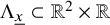 $\Lambda _{\underline {x}} \subset \mathbb {R}^2 \times \mathbb {R}$
defined by
 $$\begin{align*}\Lambda_{\underline{x}} = \left\{ (\underline{p} + q\underline{x},q) \, : \, \underline{p} \in \mathbb{Z}^2, q \in \mathbb{Z} \right\}, \end{align*}$$
we have
 $$ \begin{align} q \in Q_\Omega(\underline{x}) \iff \exists \, \underline{p} \in \mathbb{Z}^2 \text{such that} (\underline{p} + q\underline{x},q) \in \Lambda_{\underline{x}} \cap \Omega. \end{align} $$
Furthermore, since
 $c < \frac {1}{2}$
, there can be at most one
 $\underline {p} \in \mathbb {Z}^2$
for which the condition on the right-hand side holds.
According to Lemma 3.1, we have the decomposition
 $$ \begin{align} \Omega = \bigsqcup_{n \in \mathcal{F}_\Omega} a(n)^{-1}\Delta_{\Omega,n}, \end{align} $$
where the sets
 $$ \begin{align} \Delta_{\Omega,n} \subset [-c,c]^2 \times \left(\frac{a}{c^2},\frac{b e^2}{c^2} \right] \end{align} $$
are defined in (3.3), and
 $\mathcal {F}_\Omega $
is defined in (3.4)–(3.5).
Let us now fix a compactly supported Lipschitz function
 $h : \mathbb {R} \rightarrow \mathbb {R}$
. By (9.2) and (9.3),
 $$ \begin{align*} \sum_{q \in Q_\Omega(\underline{x})} h\left(\frac{q}{T}\right) &= \sum_{(\underline{p},q) \in \mathbb{Z}^2 \times \mathbb{Z}} h\left(\frac{q}{T}\right) \cdot \chi_{\Omega}(\underline{p} + q\underline{x},q) = \sum_{(\underline{\lambda}_1,\lambda_2) \in \Lambda_{\underline{x}}} h\left(\frac{\lambda_2}{T}\right) \cdot \chi_{\Omega}(\underline{\lambda}_1,\lambda_2) \\[0.2cm] &= \sum_{n \in \mathcal{F}_\Omega} \sum_{\underline{\lambda} \in \Lambda_{\underline{x}}} h\left(\frac{\lambda_2}{T}\right) \cdot \chi_{\Delta_{\Omega,n}}(a(n)\underline{\lambda}) = \sum_{n \in \mathcal{F}_\Omega} \widehat{h}_{\Omega,n}(a(n)\Lambda_{\underline{x}}), \end{align*} $$
for every
 $\underline {x} \in \mathbb {R}^2$
, where
 $$\begin{align*}h_{\Omega,n}(\underline{u},y): = h\left(\frac{e^{n_1 + n_2}y}{T}\right) \cdot \chi_{\Delta_{\Omega,n}}(\underline{u},y), \quad (\underline{u},y)\in\mathbb{R}^2\times \mathbb{R}. \end{align*}$$
By Siegel’s Theorem (Theorem 5.1), we have
 $$ \begin{align*} \int_{\mathcal{L}_3} \widehat{h}_{\Omega,n}(a(n)\Lambda) \, d\mu(\Lambda) &= \int_{\mathbb{R}} \int_{\mathbb{R}^2} h_{\Omega,n}(a(n)(\underline{u},y)) \, d\underline{u} \, dy \\[0.2cm] &= \int_{\mathbb{R}} h\left(\frac{y}{T}\right) \cdot \left( \int_{\mathbb{R}^2} \chi_{a(n)^{-1}\Delta_{\Omega,n}}(\underline{u},y) \, d\underline{u} \right) \, dy, \end{align*} $$
and thus, by (9.3),
 $$ \begin{align*} \sum_{n \in \mathcal{F}_\Omega} \int_{\mathcal{L}_3} \widehat{h}_{\Omega,n}(a(n)\Lambda) \, d\mu(\Lambda) &= \int_{\mathbb{R}} h\left(\frac{y}{T}\right) \cdot \left( \int_{\mathbb{R}^2} \sum_{n \in \mathcal{F}_\Omega }\chi_{a(n)^{-1}\Delta_{\Omega,n}}(\underline{u},y) \, d\underline{u} \right) \, dy \\[0.2cm] &= \int_{\mathbb{R}} h\left(\frac{y}{T}\right) \cdot \left(\int_{\mathbb{R}^2}\chi_{\Omega}(\underline{u},y) \, d\underline{u}\right) dy = \mathcal{M}_\Omega(h), \end{align*} $$
where
 $\mathcal {M}_\Omega (h)$
is defined in (1.3). Therefore, we conclude that
 $$ \begin{align} \sum_{q \in Q_\Omega(\underline{x})} h\left(\frac{q}{T}\right) - \mathcal{M}_\Omega(h) = \sum_{n \in \mathcal{F}_\Omega} \phi_{\Omega,n}(a(n)\Lambda_{\underline{x}}), \end{align} $$
where
 $$\begin{align*}\phi_{\Omega,n}(\Lambda) := \widehat{h}_{\Omega,n} - \int_{\mathcal{L}_3} \widehat{h}_{\Omega,n} \, d\mu. \end{align*}$$
9.3 Partial moments
To simplify notation, we write
 $$ \begin{align} D_\Omega(\Lambda) := \sum_{n \in \mathcal{F}_\Omega} \phi_{\Omega,n}(a(n)\Lambda) \end{align} $$
for a lattice
 $\Lambda $
. Our goal is to analyze convex moments of the form
 $$\begin{align*}\mathcal{C}_\Omega := \int_{\mathcal{L}_3} \theta_\kappa(D_\Omega) \, d\nu, \end{align*}$$
where the function
 $\theta _\kappa $
is defined in (1.4) and the measure
 $\nu $
on
 $\mathcal {L}_3$
is given by
 $$\begin{align*}\int_{\mathcal{L}_3} \varphi \, d\nu = \int_{[0,1)^2} \varphi(\Lambda_{\underline{x}}) \, d\underline{x}, \quad\text{for } \varphi \in C_c(\mathcal{L}_3). \end{align*}$$
The following properties of the function
 $\theta _\kappa $
can be readily verified:
-
(P1)
$\theta _\kappa $
is a convex function, increasing on
$[0,\infty )$
, and
$\theta _\kappa (t) \leq t^2$
for all t. -
(P2)
$\theta _\kappa (ct) \leq c^2 \cdot \theta _\kappa (t)$
for all
$c \geq 1$
and t. -
(P3)
$\theta _\kappa ^{-1}(u) \ll _\kappa u^{1/2} \left (\ln ^+ u \right )^{(1+\kappa )/2}$
, for all
$u\ge 0$
, where
$\ln ^+ u:=\ln \max (e,u)$
.







It will be convenient to decompose the sum (9.6) further: for
 $\xi _T < \beta _\Omega $
, we introduce the sets
 $$\begin{align*}\mathcal{G}_\Omega^{+}(\xi_T) := \left\{ n \in \mathcal{F}_\Omega \, : \, \lfloor n \rfloor \geq \xi_T \right\} \quad \text{and} \quad \mathcal{G}_\Omega^{-}(\xi_T) := \left\{ n \in \mathcal{F}_\Omega \, : \, \lfloor n \rfloor < \xi_T \right\}. \end{align*}$$
Then
 $\mathcal {F}_\Omega = \mathcal {G}_{\Omega }^{+}(\xi _T) \sqcup \mathcal {G}_{\Omega }^{-}(\xi _T)$
for all T. Let us fix
 $\varepsilon _T \in (0,1)$
and
 $L_T>1$
, and let
 $\rho _{\varepsilon _T}$
and
 $\eta _{L_T}$
be defined as in Section 8. We introduce the functions
 $$\begin{align*}f_{\Omega,n} := \rho_{\varepsilon_T} * h_{\Omega,n} \end{align*}$$
on
 $\mathbb {R}^3$
, and consider
 $$\begin{align*}\varphi_{\Omega,n} : = \widehat{f}_{\Omega,n} \cdot \eta_{L_T} - \int_{\mathcal{L}_3} \widehat{f}_{\Omega,n} \cdot \eta_{L_T} \, d\mu. \end{align*}$$
on
 $\mathcal {L}_3$
that provide a
 $C_c^\infty $
-approximation for the functions
 $\phi _{\Omega ,n}$
. We now write:
 $$ \begin{align} D_\Omega &= \sum_{n \in \mathcal{G}_\Omega^{-}(\xi_T)} \phi_{\Omega,n} \circ a(n) + \sum_{n \in \mathcal{G}_{\Omega}^{+}(\xi_T)} \left( \phi_{\Omega,n} - \varphi_{\Omega,n} \right) \circ a(n) + \sum_{n \in \mathcal{G}_{\Omega}^{+}(\xi_T)} \varphi_{\Omega,n} \circ a(n) \nonumber \\[0.2cm] &=: D_\Omega^{(1)} + D_\Omega^{(2)} + D_\Omega^{(3)}. \end{align} $$
Since
 $\theta _\kappa $
is convex and satisfies condition (P2), we have
 $$\begin{align*}\mathcal{C}_\Omega \leq 3 \cdot \left( \mathcal{C}_\Omega^{(1)} + \mathcal{C}_\Omega^{(2)} + \mathcal{C}_\Omega^{(3)} \right), \end{align*}$$
where
 $$\begin{align*}\mathcal{C}_\Omega^{(k)} := \int_{\mathcal{L}_3} \theta_\kappa\left(D_\Omega^{(k)}\right) \, d\nu, \quad \text{for } k=1,2,3. \end{align*}$$
In what follows, we will estimate these partial moments separately.
9.4 An upper bound on
$\mathcal {C}_\Omega ^{(1)}$

Since
 $\theta _\kappa $
is convex and satisfies (P2), we have
 $$ \begin{align} \mathcal{C}_\Omega^{(1)} &= \int_{\mathcal{L}_{3}}\theta_\kappa\left(\sum_{n \in \mathcal{G}^{-}_\Omega(\xi_T)} \phi_{\Omega,n} \circ a(n) \, d\nu \right) \nonumber \\[0.2cm] &\leq |\mathcal{G}^{-}_\Omega(\xi_T)|^2 \cdot \int_{\mathcal{L}_{3}}\theta_\kappa\left( \frac{1}{|\mathcal{G}^{-}_\Omega(\xi_T)|} \sum_{n \in \mathcal{G}^{-}_\Omega(\xi_T)} \phi_{\Omega,n} \circ a(n) \, d\nu \right) \nonumber \\[0.3cm] &\leq |\mathcal{G}^{-}_\Omega(\xi_T)| \cdot \sum_{n \in \mathcal{G}^{-}_\Omega(\xi_T)} \int_{\mathcal{L}_3} \theta_\kappa\big(\phi_{\Omega,n} \circ a(n)\big) \, d\nu. \end{align} $$
Furthermore,
 $$ \begin{align} \int_{\mathcal{L}_3} \theta_\kappa\big(\phi_{\Omega,n} \circ a(n)\big) \, d\nu &\leq 2 \max\left(\int_{\mathcal{L}_3} \theta_\kappa\big(\widehat{h}_{\Omega,n} \circ a(n)\big) \, d\nu, \theta_\kappa\left(\int_{\mathcal{L}_3} \widehat{h}_{\Omega,n} \, d\mu\right) \right) \end{align} $$
By Siegel’s Theorem (Theorem 5.1) and (9.4),
 $$ \begin{align} \int_{\mathcal{L}_3} \widehat{h}_{\Omega,n} \, d\mu = \int_{\mathbb{R}^2 \times \mathbb{R}} h_{\Omega,n}(\underline{u},y) \, d\underline{u} dy \leq \|h\|_\infty \operatorname{\mathrm{Vol}}_3(\Delta_{\Omega,n}) \ll_h b \ll 1. \end{align} $$
We stress that the implicit constants only depend on
 $\|h\|_\infty $
(which is assumed to be fixed throughout the proof).
Now, we observe that
 $$\begin{align*}\big|\widehat{h}_{\Omega,n}(a(n)\Lambda_{\underline{x}}) \big|\leq \|h\|_\infty \cdot \widehat{\chi}_{\Delta_{\Omega,n}}(a(n)\Lambda_{\underline{x}}), \quad \text{for all } \underline{x} \in \mathbb{R}^2. \end{align*}$$
Furthermore, by (9.4),
 $$\begin{align*}\chi_{\Delta_{\Omega,n}}(\underline{u},y) \leq \chi_{[-1,1]^2 \times [0,1]}(\underline{u},r_\Omega), \quad \text{where } r_\Omega := \frac{c^2}{b e^2}, \end{align*}$$
so we conclude that

where the lattice
 $\Lambda _{\underline {x},r_\Omega }$
is defined as in (5.3). Thus, by Lemma 5.2,
 $$ \begin{align} \big|\widehat{h}_{\Omega,n}(a(n)\Lambda_{\underline{x}})\big| \ll_h \operatorname{\mathrm{ht}}(a(n)\Lambda_{\underline{x},r_\Omega}). \end{align} $$
We note that
 $r_\Omega \geq e^{-2}\zeta $
by (9.1).
Let us now use these estimates to bound
 $\mathcal {C}_\Omega ^{(1)}$
. We introduce the set
 $$\begin{align*}E_{T,n} := \left\{ \underline{x} \in [0,1)^2 \, : \, \operatorname{\mathrm{ht}}(a(n)\Lambda_{\underline{x},r_\Omega}) \geq e^4\zeta^{-1} \right\}. \end{align*}$$
By Corollary 5.5, applied with
 $\rho =e^{-2}\zeta $
and
 $\eta = e^4\zeta ^{-1}$
, we have for all
 $n \in \mathbb {N}_o^2$
,
 $$\begin{align*}\int_{E_{T,n}} \theta_\kappa\big(\operatorname{\mathrm{ht}}(a(n)\Lambda_{\underline{x},r_\Omega})\big) \, d\underline{x} \ll_{\zeta} r_\Omega^{-1} \cdot \int_{e^2\zeta^{-1}}^{\infty} \frac{\theta_\kappa(u)}{u^3} \, du \ll_{\kappa,\zeta} r_\Omega^{-1}, \end{align*}$$
where the implicit constants are independent of T and n. Here we used that the function
 $u \mapsto \frac {\theta _\kappa (u)}{u^3}$
is integrable on
 $[1,\infty )$
. Hence, from (9.11), since
 $\theta _{\kappa }$
is increasing and satisfies (P2), we conclude that
 $$ \begin{align} \int_{E_{T,n}} \theta_\kappa\big(\widehat{h}_{\Omega,n}(a(n)\Lambda_{\underline{x}})\big) \, d\underline{x} \ll_h \int_{E_{T,n}} \theta_\kappa\big(\operatorname{\mathrm{ht}}(a(n)\Lambda_{\underline{x},r_\Omega})\big) \, d\underline{x} \ll_{\kappa,\zeta} r_\Omega^{-1}, \end{align} $$
for all n.
It remains to estimate the integral over
 $E_{T,n}^c$
. To do so, note that
 $$\begin{align*}\int_{E_{T,n}^c} \theta_\kappa\big(\widehat{h}_{\Omega,n}(a(n)\Lambda_{\underline{x}})\big) \, d\underline{x} \ll_h \int_{E_{T,n}^c \cap P_{\Omega,n}} \theta_\kappa\big(\operatorname{\mathrm{ht}}(a(n)\Lambda_{\underline{x},r_\Omega}) \big)\, d\underline{x} \ll_{\kappa,\zeta} \operatorname{\mathrm{Vol}}_2(P_{\Omega,n}), \end{align*}$$
where
 $$\begin{align*}P_{\Omega,n} : = \left\{ \underline{x} \in [0,1)^2 \, : \, \widehat{h}_{\Omega,n}(a(n)\Lambda_{\underline{x}})> 0 \right\}. \end{align*}$$
Using that
 $c < \frac {1}{2}$
, and the upper bounds, which follow from (9.4), we obtain that

we see that

where
 $s_1$
is defined as in Subsection 5.1. Hence, by Lemma 5.7, applied with
 $\varepsilon = \frac {1}{2}$
and
 $r = r_\Omega /2$
, we have
 $$\begin{align*}\operatorname{\mathrm{Vol}}_2(P_{\Omega,n}) \ll r_\Omega^{-1}, \quad \text{for all } n. \end{align*}$$
Therefore,
 $$ \begin{align*}\int_{E_{T,n}^c} \theta_\kappa\big(\widehat{h}_{\Omega,n}(a(n)\Lambda_{\underline{x}})\big) \, d\underline{x} \ll_{h,\kappa,\zeta} r_\Omega^{-1}. \end{align*} $$
If we combine this estimate with (9.10) and (9.12), we deduce from (9.9) that
 $$ \begin{align} \int_{\mathcal{L}_3} \theta_\kappa\big(\varphi_{\Omega,n} \circ a(n)\big) \, d\nu \ll_{h,\kappa,\zeta} r_\Omega^{-1}\ll \frac{b}{c^2} \end{align} $$
for all
 $n \in \mathbb {N}_o^2$
. Hence, by (9.8),
 $$ \begin{align*} \mathcal{C}_\Omega^{(1)} \leq |\mathcal{G}^{-}_\Omega(\xi_T)| \cdot \sum_{n \in \mathcal{G}^{-}_\Omega(\xi_T)} \int_{\mathcal{L}_3} \theta_\kappa\big(\varphi_{\Omega,n} \circ a(n)\big) \, d\nu \ll_{h,\kappa,\zeta} |\mathcal{G}_{\Omega}^{-}(\xi_T)|^2 \cdot \frac{b}{c^2}. \end{align*} $$
Since
 $$\begin{align*}|\mathcal{G}_\Omega^{-}(\xi_T)| \leq 2\xi_T \cdot (\beta_\Omega-\alpha_\Omega) \quad \text{and} \quad (\beta_\Omega - \alpha_\Omega)^2 \leq |\mathcal{F}_\Omega|, \end{align*}$$
we conclude that
 $$\begin{align*}|\mathcal{G}_\Omega^{-}(\xi_T)|^2 \ll \xi_T^2 \cdot |\mathcal{F}_\Omega|, \end{align*}$$
and
 $$ \begin{align} \mathcal{C}_\Omega^{(1)} \ll_{h,\kappa,\zeta} \frac{b \cdot \xi^2_T}{c^2} \cdot |\mathcal{F}_\Omega|. \end{align} $$
9.5 An upper bound on
$\mathcal {C}_\Omega ^{(2)}$

Since
 $\theta _\kappa (u) \leq u^2$
for all u, we have
 $$ \begin{align*} \int_{\mathcal{L}_3} \theta_\kappa\big(D_\Omega^{(2)}\big) \, d\nu &\leq \int_{\mathcal{L}_3} \left( \sum_{n \in \mathcal{G}_\Omega^{+}(\xi_T)} (\phi_{\Omega,n} - \varphi_{\Omega,n}) \circ a(n) \right)^2 \, d\nu \\[0.2cm] &\leq \left( \sum_{n \in \mathcal{G}_T^{+}} \big\|(\phi_{\Omega,n} - \varphi_{\Omega,n}) \circ a(n)\big\|_{L^2(\nu)}\right)^2. \end{align*} $$
Let us assume that
 $$ \begin{align} \xi_T> \max(1,-\ln\left({a}/{2}\right)). \end{align} $$
Then for all
 $n \in \mathcal {G}^{+}_\Omega (\xi _T)$
, we have
 $n_1+n_2>\max (1,-\ln \left ({a}/{2}\right ))$
. In particular, if we additionally assume that
 $$ \begin{align} \varepsilon_T<a\zeta^2/100 \quad \text{and} \quad L_T\ge 2e^2\zeta^{-1}, \end{align} $$
then the conditions of Lemma 8.5 are satisfied, from which we conclude that
 $$ \begin{align*} \big\|(\phi_{\Omega,n} - \varphi_{\Omega,n}) \circ a(n) \big\|_{L^2(\nu)} \ll_{h,\zeta}& \frac{ \varepsilon_T}{a} \cdot \max(1,n_1 + n_2)^{1/2} \\[0.2cm] &+ e^{-(n_1 + n_2)/2} + \max\Big(\varepsilon_T, -\frac{\varepsilon_T}{a} \ln\Big(\frac{\varepsilon_T}{a} \Big)\Big)^{1/2} \cdot \max(1,n_1 + n_2) \\[0.2cm] &+ \left(L_T^{-1/2} + e^{-\lfloor n \rfloor/2} \right)\cdot \max(1,n_1 + n_2)^{1/2} \end{align*} $$
for all
 $n \in \mathcal {G}^{+}_\Omega (\xi _T)$
. We note that
 $$ \begin{align*} &\sum_{n \in \mathcal{G}_\Omega^{+}(\xi_T)} \max(1,n_1 + n_2)^{1/2} \leq \beta_\Omega^{1/2} \cdot |\mathcal{G}_{\Omega}^{+}(\xi_T)|, \\[0.2cm] &\sum_{n \in \mathcal{G}_\Omega^{+}(\xi_T)} \max(1,n_1 + n_2) \leq \beta_\Omega \cdot |\mathcal{G}_{\Omega}^{+}(\xi)|, \\[0.2cm] &\sum_{n \in \mathcal{G}_\Omega^+(\xi_T)} e^{-(n_1 + n_2)/2} \le 2 e^{-\xi_T/2} \cdot |\mathcal{G}_\Omega^{+}(\xi_T)|, \\[0.2cm] &\sum_{n \in \mathcal{G}_\Omega^{+}(\xi_T)} e^{-\lfloor n \rfloor/2} \max(1,n_1 + n_2)^{1/2} \le 2 \beta_\Omega^{1/2} \cdot e^{-\xi_T/2} \cdot |\mathcal{G}_{\Omega}^{+}(\xi_T)|, \end{align*} $$
and thus
 $$ \begin{align} \int_{\mathcal{L}_3} \theta_\kappa\big(D_\Omega^{(2)}\big) \, d\nu &\leq \left(\sum_{n \in \mathcal{G}_\Omega^{+}(\xi_T)} \big\|(\phi_{\Omega,n} - \varphi_{\Omega,n}) \circ a(n)\big\|_{L^2(\nu)}\right)^2 \nonumber \\[0.2cm] &\ll_{h,\zeta} \gamma \cdot |\mathcal{G}_\Omega^{+}(\xi_T)|^2\leq \gamma\cdot\beta_\Omega^2 \cdot |\mathcal{F}_\Omega|, \end{align} $$
where
 $$\begin{align*}\gamma := \beta_\Omega \cdot \max\left( \left(\frac{\varepsilon_T}{a}\right)^2, \beta_\Omega \cdot \max \left(\varepsilon_T,-\frac{\varepsilon_T}{a} \ln\Big(\frac{\varepsilon_T}{a}\Big)\right), L_T^{-1}, e^{-\xi_T} \right). \end{align*}$$
9.6 An upper bound on
$\mathcal {C}_\Omega ^{(3)}$

We have
 $$ \begin{align} \int_{\mathcal{L}_3} \left(D_\Omega^{(3)}\right)^2 \, d\nu = & \int_{\mathcal{L}_3} \sum_{m,n \in \mathcal{G}_\Omega^{+}(\xi_T)}\varphi_{\Omega,m} \circ a(m) \cdot \varphi_{\Omega,n} \circ a(n) \, d\nu \nonumber \\ =& \sum_{\substack{m,n \in \mathcal{G}_\Omega^{+}(\xi_T) \\[0.1cm] \|m-n\| < \xi_T}} \int_{\mathcal{L}_3} \varphi_{\Omega,m} \circ a(m) \cdot \varphi_{\Omega,n} \circ a(n) \, d\nu \nonumber \\[0.2cm] &+ \sum_{\substack{m,n \in \mathcal{G}_\Omega^{+}(\xi_T) \\[0.1cm] \|m-n\| \geq \xi_T}} \int_{\mathcal{L}_3} \varphi_{\Omega,m} \circ a(m) \cdot \varphi_{\Omega,n} \circ a(n) \, d\nu. \end{align} $$
We estimate the two sums on the right-hand side separately.
By Lemma 5.2 and (9.4),
 $|\varphi _{\Omega ,n}|\ll _{h,\zeta } L_T$
for all n. Then, by the Cauchy-Schwarz inequality, we deduce
 $$ \begin{align*} & \int_{\mathcal{L}_3}\left|\varphi_{\Omega,m} \circ a(m) \cdot \varphi_{\Omega,n} \circ a(n) \right|\, d\nu \\ & \ll_{h,\zeta} (\ln L_T)^{1+\kappa}\int_{\mathcal{L}_3}\ln\left(e+|\varphi_{\Omega,m}\circ a(m)|\right)^{-(1+\kappa)/2}\cdot\left|\varphi_{\Omega,m} \circ a(m)\right| \\ &\qquad\qquad\qquad\qquad\qquad\cdot\ln\left(e+|\varphi_{\Omega,n}\circ a(n)|\right)^{-(1+\kappa)/2}\cdot \left|\varphi_{\Omega,n} \circ a(n) \right|\, d\nu \\ & \leq (\ln L_T)^{1+\kappa}\left(\int_{\mathcal{L}_3}\theta_{\kappa}(\varphi_{\Omega,m}\circ a(m))\,d\nu\cdot \int_{\mathcal{L}_3}\theta_{\kappa}(\varphi_{\Omega,n}\circ a(n))\, d\nu\right)^{1/2}. \end{align*} $$
Hence, by (9.13), we have that
 $$ \begin{align*}\int_{\mathcal{L}_3}\left|\varphi_{\Omega,m} \circ a(m) \cdot \varphi_{\Omega,n} \circ a(n)\right|\, d\nu\ll_{h,\zeta}\frac{b{\cdot(\ln L_T)^{1+\kappa}}}{c^2}.\end{align*} $$
so that
 $$ \begin{align} \sum_{\substack{m,n \in \mathcal{G}_\Omega^{+}(\xi_T) \\[0.1cm] \|m-n\| < \xi_T}} \int_{\mathcal{L}_3} \left|\varphi_{\Omega,m} \circ a(m) \cdot \varphi_{\Omega,n} \circ a(n)\right| \, d\nu\ll_{h,\zeta} \frac{b{\cdot (\ln L_T)^{1+\kappa}}}{c^2}\cdot|\mathcal{M}_\Omega(\xi_T)|, \end{align} $$
where
 $$\begin{align*}\mathcal{M}_\Omega(\xi_T) := \left\{ (m,n) \in \mathcal{G}_\Omega^{+}(\xi_T) \, : \, \|m-n\| < \xi_T \right\}. \end{align*}$$
For every
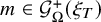 $m \in \mathcal {G}_\Omega ^{+}(\xi _T)$
, there are
 $O(\xi _T^2)$
elements n in
 $\mathcal {G}_\Omega ^{+}(\xi _T)$
such that
 $\|m-n\| < \xi _T$
, and thus
 $|\mathcal {M}_\Omega (\xi _T)| \ll \xi _T^2 \cdot |\mathcal {G}_\Omega ^{+}(\xi _T)|$
, where the implicit constants are independent of
 $\Omega $
. We thus see that
 $$ \begin{align} \sum_{\substack{m,n \in \mathcal{G}_\Omega^{+}(\xi_T) \\[0.1cm] \|m-n\| < \xi_T}} \int_{\mathcal{L}_3} \varphi_{\Omega,m} \circ a(m) \cdot \varphi_{\Omega,n} \circ a(n) \, d\nu \ll_{h,\zeta} \frac{b{\cdot (\ln L_T)^{1+\kappa}}}{c^2}\cdot \xi_T^2 \cdot |\mathcal{F}_\Omega|. \end{align} $$
Let us now turn to the second sum in (9.18). By construction, the function
 $\varphi _{\Omega ,n}$
belongs to
 $\mathbb {R} \cdot 1 + C^\infty _c(\mathcal {L}_3)$
and satisfies
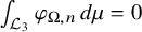 $\int _{\mathcal {L}_3} \varphi _{\Omega ,n} \, d\mu = 0$
. Hence, by Theorem 9.2, there exist
 $s \geq 1$
and
 $\delta> 0$
such that
 $$\begin{align*}\left| \int_{\mathcal{L}_3} \varphi_{\Omega,m} \circ a(m) \cdot \varphi_{\Omega,n} \circ a(n) \, d\nu \right| \ll e^{-\delta \min(\lfloor m \rfloor, \lfloor n \rfloor,\|m-n\|)} \, \mathcal{N}_s(\varphi_{\Omega,m}) \cdot \mathcal{N}_s(\varphi_{\Omega,n}), \end{align*}$$
where the implicit constants are independent of
 $m,n,T$
. Furthermore, by Lemma 8.1, there exists a constant
 $\sigma _s> 0$
such that
 $$\begin{align*}\mathcal{N}_s(\varphi_{\Omega,n}) \ll_h \varepsilon_T^{-\sigma_s} \cdot L_T, \quad \text{for all } n, \end{align*}$$
where the implicit constants are independent of
 $\Omega $
and n. We conclude that for all
 $m,n \in \mathcal {G}_\Omega ^{+}(\xi _T)$
such that
 $\|m-n\| \geq \xi _T$
, we have
 $$\begin{align*}\left| \int_{\mathcal{L}_3} \varphi_{\Omega,m} \circ a(m) \cdot \varphi_{\Omega,n} \circ a(n) \, d\nu \right| \ll_h e^{-\delta \xi_T} \cdot \varepsilon_T^{-2\sigma_s} \cdot L_T^2, \end{align*}$$
and thus
 $$ \begin{align} \sum_{\substack{m,n \in \mathcal{G}_\Omega^{+}(\xi_T) \\[0.1cm] \|m-n\| \geq \xi_T}} \int_{\mathcal{L}_3} \varphi_{\Omega,m} \circ a(m) \cdot \varphi_{\Omega,n} \circ a(n) \, d\nu \ll_h e^{-\delta \xi_T} \cdot \varepsilon_T^{-2\sigma_s} \cdot L_T^2 \cdot |\mathcal{G}_\Omega^{+}(\xi_T)|^2. \end{align} $$
If we now plug our estimates (9.20) and (9.21) into (9.18), we conclude that
 $$ \begin{align*} \int_{\mathcal{L}_3} \theta_\kappa\big(D_\Omega^{(3)}\big) \, d\nu \ll_{h,\zeta} &\frac{b\cdot(\ln L_T)^{1+\kappa}\cdot\xi_T^2}{c^2} \cdot |\mathcal{F}_\Omega| + e^{-\delta \xi_T} \cdot \varepsilon_T^{-2\sigma_s} \cdot L_T^2 \cdot |\mathcal{G}_\Omega^{+}(\xi_T)|^2. \end{align*} $$
Since
 $|\mathcal {G}_\Omega ^{+}(\xi _T)| \ll \beta _\Omega ^2$
, where the implicit constants are independent of
 $\Omega $
, we have
 $$ \begin{align} \int_{\mathcal{L}_3} \theta_\kappa\big(D_\Omega^{(3)}\big) \, d\nu \ll_{h,\zeta} \left(\frac{b\cdot (\ln L_T)^{1+\kappa}\cdot \xi_T^2}{c^2} + + e^{-\delta \xi_T} \cdot \varepsilon_T^{-2\sigma_s} \cdot L_T^2 \cdot \beta_\Omega^2 \right) \cdot |\mathcal{F}_\Omega|. \end{align} $$
9.7 Putting it all together
Let us now summarize what we have so far:
 $$\begin{align*}\mathcal{C}_\Omega \leq 3 \cdot \left(\mathcal{C}^{(1)}_\Omega + \mathcal{C}^{(2)}_\Omega + \mathcal{C}^{(3)}_\Omega \right), \end{align*}$$
and by (9.14), (9.17), (9.22),
 $$ \begin{align*} \mathcal{C}_\Omega^{(1)} &\ll_{h,\kappa,\zeta} \frac{b \cdot \xi^2_T}{c^2} \cdot |\mathcal{F}_\Omega|, \\[0.2cm] \mathcal{C}_\Omega^{(2)} &\ll_{h,\zeta} \beta_\Omega^3 \cdot \max\left( \left(\frac{\varepsilon_T}{a}\right)^2, \beta_\Omega \cdot \max\left(\varepsilon_T,-\frac{\varepsilon_T}{a} \ln\Big(\frac{\varepsilon_T}{a}\Big)\right), {L_T}^{-1}, e^{-\xi_T} \right) \cdot |\mathcal{F}_\Omega|, \\[0.2cm] \mathcal{C}_\Omega^{(3)} &{\ll_h \Big( \frac{b\cdot(\ln L_T)^{1+\kappa}\cdot \xi_T^2}{c^2} + e^{-\delta \xi_T} \cdot \varepsilon_T^{-2\sigma_s} \cdot L_T^2 \cdot \beta_\Omega^2 \Big) \cdot |\mathcal{F}_\Omega|}, \end{align*} $$
provided that the parameters have been chosen so that
 $$ \begin{align} \xi_T \geq \max(1,-\ln\left({a}/{2}\right)),\quad \varepsilon_T<a\zeta^2/100, \quad L_T\ge e^2\zeta^{-1},\quad c^2>\zeta\cdot b. \end{align} $$
We further assume that
 $$\begin{align*}a \geq (\ln T)^{-\theta}, \quad \text{for some } \theta> 0. \end{align*}$$
Then, in particular,
 $\beta _\Omega = \ln \left (\frac {Tc^2}{a}\right )\ll _{\theta } \ln T.$
In what follows, we will choose the parameters
 $\xi _T, \varepsilon _T$
, and
 $L_T$
, so that
 $$ \begin{align} \mathcal{C}_\Omega \ll_{h,\kappa,\zeta} \left(\frac{b\cdot(\ln L_T)^{1+\kappa} \cdot \xi_T^2}{c^2} + O_{\theta,\rho}\big((\ln T)^{-\rho}\big)\right) \cdot |\mathcal{F}_\Omega| \end{align} $$
for all
 $\rho>0$
.
To prove (9.24), let
 $$\begin{align*}\xi_T = \xi_o \cdot \ln(\ln T), \quad L_T = (\ln T)^{3 + \eta}, \quad \varepsilon_T = (\ln T)^{-\gamma} \end{align*}$$
for some positive constants
 $\xi _o, \eta $
and
 $\gamma $
that will be chosen later. With these choices, we see that
 $$ \begin{align*} \beta^3_\Omega \cdot \left(\frac{ \varepsilon_T}{a}\right)^2 &\ll_{\theta} (\ln T)^{3 - 2(\gamma-\theta)}, \\[0.2cm] \beta_\Omega^4 \cdot \max \left(\varepsilon_T,-\frac{\varepsilon_T}{a} \ln\Big(\frac{\varepsilon_T}{a}\Big)\right) &\ll_{\theta} (\ln T)^{4-(\gamma-\theta)} \cdot \ln(\ln T), \\[0.4cm] \beta_\Omega^3\cdot \max\left({L_T}^{-1}, e^{-\xi_T} \right) &\ll_{\theta} \max\left((\ln T)^{-\eta},(\ln T)^{3-\xi_o} \right), \\[0.4cm] e^{-\delta \xi_T} \cdot \varepsilon_T^{-2\sigma_s} \cdot L_T^2 \cdot \beta_\Omega^2 &\ll_{\theta} (\ln T)^{-\delta \xi_o + 2\sigma_s \gamma + 2(3+\eta) + 2}, \end{align*} $$
for all sufficiently large T. We think of
 $\theta $
as fixed throughout the argument. Hence, if we pick
 $\eta , \gamma $
sufficiently large and next
 $\xi _o$
sufficiently large, then all of the right-hand sides above are
 $O_{\theta ,\rho }((\ln T)^{-\rho })$
for any
 $\rho>0$
. Furthermore, one verifies that all the conditions in (9.23) are satisfied. Hence, (9.24) follows. Since
 $$ \begin{align*}\frac{b}{c^2}\gg a \ge (\ln T)^{-\theta}, \end{align*} $$
we obtain that
 $$ \begin{align} \mathcal{C}_\Omega \ll_{h,\kappa,\zeta,\theta} \frac{b \cdot (\ln L_T)^{1+\kappa}\cdot \xi_T^2}{c^2} \cdot |\mathcal{F}_\Omega|. \end{align} $$
Furthermore,
 $$ \begin{align*}\xi_{T}\ll \ln\ln T\quad \text{and} \quad |\mathcal{F}_\Omega|\ll \beta_\Omega^2-\alpha_\Omega^2, \end{align*} $$
where
 $$ \begin{align*}\alpha_\Omega=\ln \left(\frac{T_0 c^2}{e^2b} \right) \quad \text{and} \quad \beta_\Omega=\ln \left(\frac{T c^2}{a} \right). \end{align*} $$
Since, according to our assumptions,
 $$ \begin{align*}\zeta\le \frac{c^2}{b}<\frac{c^2}{a}\le (\ln T)^{\theta}, \end{align*} $$
we conclude that
 $$ \begin{align*} |\mathcal{F}_\Omega|\ll \left(\ln T+ \ln \left(\frac{ c^2}{a} \right)\right)^2-\left(\ln T_0 +\ln \left(\frac{c^2}{e^2b} \right)\right)^2 \ll_\zeta \mathcal{L}([T_0,T)) + \mathcal{M}([T_0,T)), \end{align*} $$
where
 $$ \begin{align*}\mathcal{L}([T_0,T)):=(\ln T)^2- (\ln T_0)^2\quad\text{and}\quad \mathcal{M}([T_0,T)):=\ln T\ln\ln T. \end{align*} $$
Hence, it follows from (9.5) and (9.25) that
 $$ \begin{align} \int_{[0,1)^2} \theta_\kappa\Big( S_\Omega h(\underline{x})-\mathcal{M}_\Omega(h) \Big)\, d\underline{x}&=\int_{\mathcal{L}_3} \theta_\kappa\left(D_\Omega\right)\, d\nu \nonumber \\ & \ll_{h,\kappa,\zeta,\theta} c^{-2}\cdot b\cdot (\ln\ln T)^{3+\kappa}\cdot \Big( \mathcal{L}([T_0,T)) + \mathcal{M}([T_0,T))\Big). \end{align} $$
In particular, in the case when
 $T_0=1$
, we obtain Theorem 1.3.
10 Proof of Theorem 1.2
We work with the sets
 $$ \begin{align*}\Omega=\Omega^{(a,b],c}_{[T_0,T)} := \left\{ (u,y) \in \mathbb{R}^2 \times [T_0,T) \, : \, \begin{array}{c} \max(|u_1|,|u_2|) \leq c \\[0.2cm] a < |u_1u_2| \cdot y \leq b \end{array} \right\} \end{align*} $$
that depend on parameters
 $0<a<b<1$
,
 $0<c<1/2$
,
 $1\le T_0<T$
. For a lattice
 $\Lambda $
, we consider the discrepancy function
 $$ \begin{align*}D^{(a,b],c}_{[T_0,T)}(\Lambda):=\left|\Lambda\cap \Omega^{(a,b],c}_{[T_0,T)}\right|-\operatorname{\mathrm{Vol}}_3\left(\Omega^{(a,b],c}_{[T_0,T)}\right). \end{align*} $$
Let us take in (9.26) a Lipschitz function h such that
 $h=1$
on
 $[0,1]$
. Then
 $$ \begin{align*}S_\Omega h(\underline{x})= \left|\Lambda_{\underline{x}}\cap \Omega\right|\quad \text{and} \quad \mathcal{M}_\Omega (h) =\operatorname{\mathrm{Vol}}_3(\Omega), \end{align*} $$
so that it follows that
 $$ \begin{align} \int_{\mathcal{L}_3} \theta_\kappa\left(\left|D^{(a,b],c}_{[T_0,T)}\right|\right)\, d\nu \ll_{\kappa,\zeta,\theta} c^{-2}\cdot b\cdot (\ln\ln T)^{3+\kappa}\cdot \Big( \mathcal{L}([T_0,T)) + \mathcal{M}([T_0,T))\Big). \end{align} $$
We use this estimate for a Borel–Cantelli argument below.
For
 $s \in \mathbb {N}$
, let us denote by
 $\mathcal {I}_s$
the collection of intervals
 $$ \begin{align} I_{i,j}: = \left[e^{2^i j}, e^{2^{i}(1+j)}\right). \end{align} $$
with
 $(i,j) \in \mathbb {N}_o^2$
satisfying
 $2^i (1+j) < 2^s$
. The following lemma is essentially [Reference Schmidt16, Lemma 1], although this lemma takes place in a slightly different setting. We provide a proof of our version for completeness.
Lemma 10.1. For every
 $1 \leq N < 2^s$
, there exists a subset
 $\mathcal {H}_N \subset \mathcal {I}_s$
such that
 $$\begin{align*}|\mathcal{H}_N| \leq s \quad \text{and} \quad [1,e^N) = \bigsqcup_{I \in \mathcal{H}_N} I. \end{align*}$$
Proof. We write
 $$\begin{align*}N = \sum_{k=1}^p 2^{n_k}, \end{align*}$$
where
 $0 \leq n_1 < n_2 < \ldots < n_p < s$
are integers. In particular,
 $p \leq s$
. Let
 $$\begin{align*}N_0 = 0 \quad \text{and} \quad N_m = \sum_{k=p - m + 1}^{p} 2^{n_k}, \quad \text{for } m = 1,\ldots,p, \end{align*}$$
so that
 $N_p = N$
and
 $$\begin{align*}[1,e^N) = \bigsqcup_{m=1}^{p} [e^{N_{m-1}},e^{N_m}). \end{align*}$$
We claim that each interval
 $[e^{N_{k}},e^{N_{k+1}})$
for
 $k=0,\ldots ,p-1$
is of the form
 $I_{i,j}$
for some index pair
 $(i,j) \in \mathcal {G}_s$
. To see this, first note that
 $[1,e^{N_1}) = I_{i_1,j_1}$
, where
 $i_1 = n_p$
and
 $j_1 = 0$
. More generally, we see that
 $$\begin{align*}N_{m+1} = 2^{n_{p-m}} + \ldots + 2^{n_{p}} = 2^{n_{p-m}}\left(1 + 2^{n_{p-m+1}-n_{p-m}} + \ldots + 2^{n_p - n_{p-m}} \right). \end{align*}$$
Hence, if we define
 $$\begin{align*}i_m = n_{p-m} \quad \text{and} \quad j_{m} = 2^{n_{p-m+1}-n_{p-m}} + \ldots + 2^{n_p - n_{p-m}} \end{align*}$$
for
 $1 \leq m \leq p-1$
, then
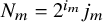 $N_m = 2^{i_m} j_m$
and
 $N_{m+1} = 2^{i_m}(1 + j_m)$
, and thus
 $[e^{N_{m}},e^{N_{m+1}}) = I_{i_m,j_m}$
. In particular,
 $$\begin{align*}[1,e^N) = \bigsqcup_{m=1}^p I_{i_m,j_m}. \end{align*}$$
so that we establish the lemma with
 $\mathcal {H}_N := \{ I_{i_m,j_m} \, : \, 1 \leq m \leq p \}$
.
Lemma 10.2. For every
 $s\in \mathbb {N}$
,
 $$\begin{align*}|\mathcal{I}_s|\ll 2^s,\quad\quad \sum_{I \in \mathcal{I}_s} \mathcal{L}(I) \ll s \cdot 2^{2s}, \quad\quad \sum_{I \in \mathcal{I}_s} \mathcal{M}(I) \ll s \cdot 2^{2s}. \end{align*}$$
Proof. We have
 $$\begin{align*}\mathcal{L}(I_{i,j}) = (2^i j + 2^i)^2-(2^i j)^2\ll 2^{2i} \cdot \max(1,j), \end{align*}$$
and
 $$ \begin{align*}\mathcal{M}(I_{i,j}) \le s\cdot 2^i(j+1), \end{align*} $$
so that
 $$\begin{align*}\sum_{I \in \mathcal{I}_s} \mathcal{L}(I) \ll \sum_{i=0}^s 2^{2i} \left( \sum_{j=0}^{2^{s-i} -1} \max(1,j) \right) \ll \sum_{i=0}^s 2^{2i} \, (2^{s-i})^{2} \ll s \cdot 2^{2s}, \end{align*}$$
and
 $$ \begin{align*}\sum_{I \in \mathcal{I}_s} \mathcal{M}(I) \ll s\cdot \sum_{i=0}^s 2^{i} \left( \sum_{j=0}^{2^{s-i} -1} (j+1) \right) \ll s\cdot \sum_{i=0}^s 2^{i} \, (2^{s-i})^{2} \ll s \cdot 2^{2s}, \end{align*} $$
as required.
We note that later in the argument below, we choose the parameters N and s so that
 $e^{N-1}\le T < e^N$
and
 $2^{s-1}\le N < 2^s$
, so that
 $\ln T\ll 2^s\ll \ln T$
.
We also use a similar argument to decompose the intervals
 $(a,b]$
. For
 $M\in \mathbb {N}$
and
 $v\in \mathbb {N}$
, we write
 $$ \begin{align*}a_M:=M^{-\sigma}\quad \text{and} \quad b_v:=2^{-v}\quad\text{with } \sigma>0. \end{align*} $$
Let
 $t\in \mathbb {N}$
. For
 $(i,j) \in \mathbb {N}_o\times \mathbb {N}$
satisfying
 $2^i (1+j) < 2^t$
, we set
 $$ \begin{align} J_{i,j}: = \left( (2^{i}(1+j))^{-\sigma},(2^i j)^{-\sigma}\right], \end{align} $$
and for
 $i=1,\ldots ,t-1$
,
 $$ \begin{align} J_{i,0}: = \left( 2^{-\sigma i},1\right]. \end{align} $$
Additionally, we subdivide each of those intervals into smaller intervals using the points
 $b_v$
with
 $v=1,\ldots , t-1$
. Let us denote the collection of all intervals that we obtain in this way by
 $\mathcal {J}_t$
. Since each of the original intervals
 $J_{i,j}$
is subdivided into at most t subintervals, the following lemma follows immediately from Lemma 10.1.
Lemma 10.3. For every
 $M\in \mathbb {N}$
with
 $2 \leq M < 2^t$
and
 $v\in \mathbb {N}$
with
 $M^{-\sigma }<2^{-v}$
, there exists a subset
 $\mathcal {G}_{M,v} \subset \mathcal {J}_t$
such that
 $$\begin{align*}|\mathcal{G}_{M,v}| \leq t^2 \quad \text{and} \quad (a_M,b_v] = \bigsqcup_{J \in \mathcal{G}_{M,v}} J. \end{align*}$$
Additionally, we note that
Lemma 10.4. Let
 $\rho \in (0,1)$
and
 $\sigma \ge \rho ^{-1}$
. Then for every
 $t\in \mathbb {N}$
,
 $$\begin{align*}|\mathcal{J}_t|\ll t\cdot 2^t\quad\text{and}\quad \sum_{(a,b]\in\mathcal{J}_t} b^{\rho}\ll t. \end{align*}$$
Proof. We note that the number of the intervals
 $J_{i,j}$
is
 $O(2^t)$
. Since each of them is subdivided into at most t subintervals, the first estimate follows. Regarding the second estimate, we observe that the sum over intervals obtained from the subdivision of the interval
 $(u_1,u_2]=J_{i,j}$
is
 $O(u_2^{1/2})$
, so that
 $$ \begin{align*} \sum_{(a,b]\in\mathcal{J}_t} b^{\rho}&\ll \sum_{i=0}^t \left(\sum_{j=1}^{2^{t-i} -1} (2^i j)^{-\sigma\rho}+1\right)\ll \sum_{i=0}^t 2^{-i\sigma\rho}\cdot 2^{(t-i)(1-\sigma \rho)} +t \ll t, \end{align*} $$
which proves the lemma.
We recall our assumption that
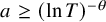 $a\ge (\ln T)^{-\theta }$
. Later in the proof, we pick an integer M such that
 $a_M\le a< a_{M-1}$
and
 $M<2^t$
, so that we may take the parameter t satisfying
 $(2^t-1)^\sigma \le (\ln T)^{\theta }$
, in particular,
 $t\ll \ln \ln T\ll s$
.
To interpolate the parameter c, we use
 $$ \begin{align*}c_w:=2^{-w} \quad \text{with } w\in \mathbb{N}. \end{align*} $$
According to our assumptions,
 $c\ge \zeta ^{1/2} (\ln T)^{-\theta /2}$
, so that it is sufficient to consider
 $w\le r$
with
 $r=O(\ln \ln T)$
, in particular,
 $r\ll s$
.
With these prerequisites, we are ready to set up a Borel–Cantelli argument. Let us fix
 $\kappa , \varepsilon> 0$
,
 $\rho \in (0,1)$
,
 $\sigma \ge \rho ^{-1}$
, and an integer
 $s \geq 2$
. Let
 $t(s),r(s)\in \mathbb {N}$
such that
 $t(s)\ll s$
and
 $r(s)\ll s$
. We set
 $$ \begin{align} X_{s} : = \left\{ \Lambda\in\mathcal{L}_3 \, : \, \sum_{w\le r(s)} \sum_{I \in \mathcal{I}_s}\sum_{(a,b]\in\mathcal{J}_{t(s)}} c_w^2 \cdot b^{-(1-\rho)}\cdot \theta_\kappa\left(\left|D^{(a,b], c_w}_{I}(\Lambda)\right|\right) \geq s^{7+\kappa+\varepsilon} \cdot 2^{2s} \right\} \end{align} $$
Then from Chebyshev’s inequality and (10.1),
 $$ \begin{align*} \nu(X_s) &\leq \frac{1}{s^{7+\varepsilon}\cdot 2^{2s} } \sum_{w\le r(s)} \sum_{I \in \mathcal{I}_s}\sum_{(a,b]\in\mathcal{J}_{t(s)}} c_w^2\cdot b^{-(1-\rho)} \int_{\mathcal{L}_3} \theta_\kappa\left(\left|D^{(a,b], c_w}_{I}\right|\right) \, d\nu\\ &\ll_{\kappa,\zeta,\theta} \frac{s^{4+\kappa}}{s^{7+\kappa+\varepsilon} \cdot 2^{2s} } \left(\sum_{I \in \mathcal{I}_s} \big(\mathcal{L}(I)+\mathcal{M}(I)\big)\right) \left(\sum_{(a,b]\in\mathcal{J}_{t(s)}} b^{\rho}\right). \end{align*} $$
Hence, it follows from Lemmas 10.2 and 10.4 that
 $$ \begin{align} \nu(X_s) \ll s^{-(1+\varepsilon)}. \end{align} $$
Let us take an integer
 $1 \leq N < 2^s$
,
 $1 \leq M < 2^{t}$
, and
 $v\in \mathbb {N}$
such that
 $1/M<2^{-v}$
. We use the partitions of the intervals
 $[1,e^N)$
and
 $(a_M,b_v]$
provided by Lemmas 10.1 and 10.3. Then
 $$\begin{align*}\left|D^{(a_M,b_v], c_w}_{[1,e^N)}\right| = \left| \sum_{I\in \mathcal{H}_N} \sum_{J \in \mathcal{G}_{M,v}} D^{J, c_w}_{I} \right| \leq \frac{1}{|\mathcal{H}_N||\mathcal{G}_{M,v}|} \sum_{I\in \mathcal{H}_N} \sum_{J \in \mathcal{G}_{M,v}} |\mathcal{H}_N||\mathcal{G}_{M,v}| \cdot \left|D^{J, c_w}_{I}\right|. \end{align*}$$
Since
 $\theta _\kappa $
is increasing, convex and satisfies the property (P2), we have
 $$ \begin{align*} \theta_\kappa\left(\left|D^{(a_M,b_v], c_w}_{[1,e^N)}\right|\right) &\leq \theta_\kappa\left(\frac{1}{|\mathcal{H}_N||\mathcal{G}_{M,v}|} \sum_{I\in \mathcal{H}_N}\sum_{J \in \mathcal{G}_{M,v}} |\mathcal{H}_N||\mathcal{G}_{M,v}| \cdot \left|D^{J, c_w}_{I}\right|\right) \\[0.2cm] &\leq \frac{1}{|\mathcal{H}_N||\mathcal{G}_{M,v}|} \sum_{I\in \mathcal{H}_N}\sum_{J\in \mathcal{G}_{M,v}} \theta_\kappa\left(|\mathcal{H}_N||\mathcal{G}_{M,v}| \cdot \left|D^{J, c_w}_{I}\right| \right) \\[0.3cm] &\leq |\mathcal{H}_N||\mathcal{G}_{M,v}| \cdot \sum_{I\in \mathcal{H}_N}\sum_{J \in \mathcal{G}_{M,v}} \theta_\kappa\left(\left|D^{J, c_w}_{I}\right|\right) \ll s^3 \cdot \sum_{I\in \mathcal{H}_N}\sum_{J \in \mathcal{G}_{M,v}} \theta_\kappa\left(\left|D^{J, c_w}_{I}\right|\right), \end{align*} $$
where we have used the property (P2) with
 $c = |\mathcal {H}_N| |\mathcal {G}_{M,v}|\le s\cdot t(s)^2\ll s^3$
in the last third inequality. This also implies that
 $$ \begin{align*}b_v^{-(1-\rho)}\cdot \theta_\kappa\left(\left|D^{(a_M,b_v], c_w}_{[1,e^N)}\right|\right) \ll s^3 \cdot \sum_{I\in \mathcal{H}_N}\sum_{(a,b] \in \mathcal{G}_{M,v}} b^{-(1-\rho)}\cdot\theta_\kappa\left(\left|D^{J, c_w}_{I}\right|\right). \end{align*} $$
Therefore, for
 $\Lambda \notin X_s$
,
 $$\begin{align*}\theta_\kappa\left(\left|D^{(a_M,b_v], c_w}_{[1,e^N)}(\Lambda)\right|\right) \ll c_w^{-2}\cdot b_v^{1-\rho}\cdot s^{10+\kappa+\varepsilon} \cdot 2^{2s}. \end{align*}$$
Then by the property (P3),
 $$ \begin{align} \left|D^{(a_M,b_v], c_w}_{[1,e^N)}(\Lambda)\right| &\ll_\kappa c_w^{-1}\cdot b_v^{(1-\rho)/2} \cdot s^{(10+\kappa+\varepsilon)/2} \cdot 2^{s} \cdot \left(\ln^+\left(c_w^{-2}\cdot b^{1-\rho} \cdot s^{10+\kappa+\varepsilon} \cdot 2^{s} \right) \right)^{(1+\kappa)/2} \nonumber \\[0.2cm] &\ll c_w^{-1}\cdot b_v^{(1-\rho)/2}\cdot \left( \ln^+ \left(c_w^{-2}\cdot b_v^{1-\rho}\right) \right)^{(1+\kappa)/2} s^{11/2+(2\kappa+\varepsilon)/2} \cdot \left( \ln s \right)^{(1+\kappa)/2} \cdot 2^{s} \nonumber \\ &\ll_\zeta c_w^{-1}\cdot b_v^{(1-\rho)/2}\cdot s^{6+(3\kappa+\varepsilon)/{2}} \cdot \left( \ln s \right)^{1+\kappa} \cdot 2^{s}. \end{align} $$
for all
 $s \geq 2$
and
 $\Lambda \notin X_s$
, where we have used that
 $$\begin{align*}\ln^+(x_1 \cdot x_2) \leq 2\cdot \ln^+ x_1 \cdot \ln^+ x_2 , \quad \text{for all } x_1,x_2\ge 0, \end{align*}$$
and our assumption on parameters v and w. Since
 $\varepsilon ,\kappa> 0 $
are arbitrary, the last estimate can be restated as: for all
 $\varepsilon> 0$
,
 $s\ge 2$
, and
 $\Lambda \notin X_s$
,
 $$ \begin{align} \left|D^{(a_M,b_v], c_w}_{[1,e^N)}(\Lambda)\right| &\ll_{\zeta,\varepsilon} c_w^{-1}\cdot b_v^{(1-\rho)/2}\cdot s^{6+\varepsilon} \cdot 2^{s}. \end{align} $$
Since by (10.6)
 $$\begin{align*}\sum_{s \geq 2} \nu(X_s) < \infty, \end{align*}$$
it follows from Borel-Cantelli’s Lemma that there exists a conull Borel set
 $\Psi \subset [0,1)^2$
and a measurable map
 $s_o : \Psi \rightarrow \mathbb {N}$
such that for all
 $\underline {x} \in \Psi $
and
 $s \geq s_o(\underline {x})$
, we have
 $\Lambda _{\underline {x}} \notin X_s$
and the estimate (10.8) holds:
 $$ \begin{align} \left|D^{(a_M,b_v], c_w}_{[1,e^N)}(\Lambda_{\underline{x}})\right| \ll_{\zeta,\varepsilon} c_w^{-1}\cdot b_v^{1-\rho} \cdot s^{6+\varepsilon} \cdot 2^{s} , \end{align} $$
for all integers
 $1 \leq N < 2^s$
,
 $1 \leq M < 2^{t(s)}$
, v such that
 $1/M<2^{-v}$
, and
 $w\le r(s)$
.
Now for general
 $T\ge 1$
, we denote by
 $N_T$
the positive integer such that
 $$ \begin{align*}e^{N_T-1} \leq T < e^{N_T}. \end{align*} $$
We apply the above estimate with
 $$ \begin{align*}s=\lfloor\log_2(N_T+1)\rfloor+1,\quad t=\lfloor\log_2\big((\ln T)^{\theta/\sigma}+1\big)\rfloor+1,\quad r=\lfloor\log_2\big(\zeta^{-1/2}(\ln T)^{\theta/2}\big)\rfloor+1, \end{align*} $$
so that
 $$ \begin{align*}2^s\ll N_T,\quad 2^t\ll N_T^{\theta/\sigma},\quad r\ll s. \end{align*} $$
Let
 $$\begin{align*}T_o(\underline{x}) := \min\big\{ T \geq 1 \, : \, \lfloor\log_2(N_T+1)\rfloor \geq s_o(\underline{x}) \big\}. \end{align*}$$
For
 $a\in ((\ln T)^{-\theta }, 1)$
, we pick an integer
 $M<2^{t}$
such that
 $$ \begin{align*}a_M\le a< a_{M-1}. \end{align*} $$
Note that then
 $$ \begin{align*}a_{M-1}-a_M\ll M^{-1-\sigma}\ll a^{1+\sigma^{-1}}. \end{align*} $$
For the parameter
 $c\in (0,1/2)$
satisfying
 $c\ge \zeta ^{1/2} (\ln T)^{-\theta /2}$
we choose
 $w\le r$
such that
 $$ \begin{align*}c_{w}\le c <c_{w-1}. \end{align*} $$
We observe that
 $$ \begin{align*}\Omega^{(a_{M-1},b_v], c_{w}}_{[1,e^{N_T-1})}\subset \Omega^{(a,b_v], c}_{[1,T)}\subset \Omega^{(a_M,b_v], c_{w-1}}_{[1,e^{N_T})}. \end{align*} $$
In particular,
 $$ \begin{align*} \left|\Lambda\cap \Omega^{(a,b_v], c}_{[1,T)}\right|\le \left|\Lambda\cap \Omega^{(a_M,b_v], c_{w-1}}_{[1,e^{N_T})}\right|, \end{align*} $$
so that
 $$ \begin{align*}D^{(a,b_v], c}_{[1,T)}\le D^{(a_M,b_v], c_{w-1}}_{[1,e^{N_T})}+\operatorname{\mathrm{Vol}}_3\left(\Omega^{(a_{M},b_v], c_{w-1}}_{[1,e^{N_T})}\right)-\operatorname{\mathrm{Vol}}_3\left(\Omega^{(a_{M-1},b_v], c_{w}}_{[1,e^{N_T-1})}\right). \end{align*} $$
According to the volume estimates from Lemma A.1,
 $$ \begin{align*} \operatorname{\mathrm{Vol}}_3\left(\Omega^{(a_{M},b_v], c_{w-1}}_{[1,e^{N_T})}\right)&= 2 N_T^2 (b_v-a_{M})+O_{\zeta,\theta}\Big( \ln T (\ln\ln T) (b_v-a_{M})+1\Big), \end{align*} $$
and
 $$ \begin{align*} \operatorname{\mathrm{Vol}}_3\left(\Omega^{(a_{M-1},b_v], c_{w}}_{[1,e^{N_T-1})}\right) &= 2 (N_T-1)^2 (b_v-a_{M-1})+O_{\zeta,\theta}\Big( \ln T (\ln\ln T) (b_v-a_{M-1})+1\Big). \end{align*} $$
Then
 $$ \begin{align*} \operatorname{\mathrm{Vol}}_3\left(\Omega^{(a_{M},b_v], c_{w-1}}_{[1,e^{N_T})}\right)-\operatorname{\mathrm{Vol}}_3\left(\Omega^{(a_{M-1},b_v], c_{w}}_{[1,e^{N_T-1})}\right) &\ll_{\zeta,\theta} N_T^2 (a_{M-1}-a_M)+N_T b_v+ \ln T (\ln\ln T) b_v+1\\ &\ll (\ln T)^2 a^{1+\sigma^{-1}} + \ln T (\ln\ln T) b_v+1. \end{align*} $$
Applying (10.9), we obtain that for
 $\underline {x}\in \Psi $
and
 $T\ge T_o(\underline {x})$
,
 $$ \begin{align*} \left|D^{(a_M,b_v], c_w}_{[1,e^{N_T})}(\Lambda_{\underline{x}})\right| \ll_{\zeta,\varepsilon} c_w^{-1}\cdot b_v^{(1-\rho)/2} \cdot (\ln N_T)^{6+\varepsilon} \cdot \ln T. \end{align*} $$
Combining those estimates, we conclude that
 $$ \begin{align*} D^{(a,b_v], c}_{[1,T)}(\Lambda_{\underline{x}}) \ll_{\zeta, \theta,\varepsilon} (\ln T)^2 a^{1+\sigma^{-1}}+c^{-1}\cdot b_v^{(1-\rho)/2} \cdot (\ln \ln T)^{6+\varepsilon} \cdot \ln T+1 \end{align*} $$
for sufficiently large T. The lower bound on
 $D^{(a,b_v], c}_{[1,T)}$
is proved similarly. Ultimately, we conclude that
 $$ \begin{align*} \left|\Lambda_{\underline{x}}\cap \Omega^{(a,b_v],c}_{[1,T)}\right| =&\operatorname{\mathrm{Vol}}_3\left(\Omega^{(a,b_v],c}_{[1,T)}\right)\\ &+O_{\zeta, \theta, \varepsilon}\left( (\ln T)^2 a^{1+\sigma^{-1}}+c^{-1}\cdot b_v^{(1-\rho)/2} \cdot (\ln \ln T)^{6+\varepsilon} \cdot \ln T+1 \right) \end{align*} $$
for sufficiently large T.
Finally, for
 $b\in (a,1)$
, we pick
 $v\le t$
such that
 $b_v\le b< b_{v-1}$
. Since
 $$ \begin{align*}\left|\Lambda_{\underline{x}}\cap \Omega^{(a,b],c}_{[1,T)}\right| =\left|\Lambda_{\underline{x}}\cap \Omega^{(a,b_{v-1}],c}_{[1,T)}\right|- \left|\Lambda_{\underline{x}}\cap \Omega^{(b,b_{v-1}],c}_{[1,T)}\right|, \end{align*} $$
and
 $$ \begin{align*}\operatorname{\mathrm{Vol}}_3\left(\Omega^{(a,b],c}_{[1,T)}\right)= \operatorname{\mathrm{Vol}}_3\left(\Omega^{(a,b_{v-1}],c}_{[1,T)}\right)- \operatorname{\mathrm{Vol}}_3\left(\Omega^{(b,b_{v-1}],c}_{[1,T)}\right), \end{align*} $$
we deduce that
 $$ \begin{align*} \left|\Lambda_{\underline{x}}\cap \Omega^{(a,b],c}_{[1,T)}\right| =&\operatorname{\mathrm{Vol}}_3\left(\Omega^{(a,b],c}_{[1,T)}\right)\\ &+O_{\zeta, \theta, \varepsilon}\left( (\ln T)^2 \cdot b^{1+\sigma^{-1}}+c^{-1}\cdot b^{(1-\rho)/2} \cdot (\ln \ln T)^{6+\varepsilon} \cdot \ln T+1 \right) \end{align*} $$
for sufficiently large T. We recall that
 $\sigma \ge \rho ^{-1}$
, so that we get the best estimate when
 $\sigma = \rho ^{-1}$
:
 $$ \begin{align*} \left|\Lambda_{\underline{x}}\cap \Omega^{(a,b],c}_{[1,T)}\right| =&\operatorname{\mathrm{Vol}}_3\left(\Omega^{(a,b],c}_{[1,T)}\right)\\ &+O_{\zeta,\theta,\varepsilon}\left( (\ln T)^2\cdot b^{1+\rho}+c^{-1}\cdot b^{(1-\rho)/2} \cdot (\ln \ln T)^{6+\varepsilon} \cdot \ln T+1 \right). \end{align*} $$
Let us suppose that
 $b\le (c\cdot \ln T)^{-2/(3\rho +1)}.$
Then one checks by a direct computation that the second summand in the error term dominates the first summand, so that we get
 $$ \begin{align*} \left|\Lambda_{\underline{x}}\cap \Omega^{(a,b],c}_{[1,T)}\right| =\operatorname{\mathrm{Vol}}_3\left(\Omega^{(a,b],c}_{[1,T)}\right) +O_{\zeta,\theta, \varepsilon}\left( c^{-1}\cdot b^{(1-\rho)/2} \cdot (\ln \ln T)^{6+\varepsilon} \cdot \ln T+1 \right) \end{align*} $$
for
 $T\ge T_o(\underline {x})$
. This provides a nontrivial estimate when
 $b\ge (c\cdot \ln T)^{-2/(\rho +1)}.$
On the other hand, when
 $b\ge (c\cdot \ln T)^{-2/(3\rho +1)},$
we get the bound:
 $$ \begin{align*} \left|\Lambda_{\underline{x}}\cap \Omega^{(a,b],c}_{[1,T)}\right| =\operatorname{\mathrm{Vol}}_3\left(\Omega^{(a,b],c}_{[1,T)}\right) +O_{\zeta,\theta, \varepsilon}\left( b^{1+\rho}\cdot(\ln \ln T)^{6+\varepsilon}\cdot (\ln T)^2+1\right) \end{align*} $$
for
 $T\ge T_o(\underline {x})$
. These estimates hold for all T with explicit constant depending on
 $\underline {x}$
. This gives Theorem 1.2 by choosing
 $\eta =2/(\rho +1)$
.
11 Proof of Theorem 1.1
To prove the corollary, we investigate existence of points in lattices
 $$ \begin{align*}\Lambda_{\underline{x}} = \{ (\underline{p} + q\underline{x},q) \in \mathbb{R}^2 \times \mathbb{R} \, : \, (\underline{p},q) \in \mathbb{Z}^2 \times \mathbb{Z} \} \end{align*} $$
contained in very thin hyperbolic strips. For
 $T \geq 1$
, let
 $a_{T}$
be a positive function of T. We consider the domains
 $$ \begin{align} \Upsilon_T := \left\{ (\underline{u},y) \in \mathbb{R}^2 \times \mathbb{R} \, : \, |u_1u_2| \cdot y \leq a_{T}, \max(|u_1|,|u_2|) \leq \frac{1}{2}, 1 \leq y < T \right\}. \end{align} $$
Our main result in this section reads as follows.
Lemma 11.1. Suppose that
 $a_{T}$
is nonincreasing and
 $a_{T}=o((\ln T)^{-2})$
as
 $T\to \infty $
. Then there is a conull set
 $Z \subset [0,1)^2$
and a measurable function
 $T : Z \rightarrow [1,\infty )$
such that for every
 $\underline {x} \in Z$
,
 $$\begin{align*}\Lambda_{\underline{x}} \cap \Upsilon_T = \emptyset, \quad \text{for all } T \geq T(\underline{x}). \end{align*}$$
Proof. By our assumption on a, the family
 $(\Upsilon _T)$
is decreasing. Hence, if we can show that for almost every
 $\underline {x} \in [0,1)^2$
, there is
 $T(\underline {x}) \geq 1$
such that
 $\Lambda _{\underline {x}} \cap \Upsilon _{T(\underline {x})} = \emptyset $
, the lemma is established. Let us consider the counting function
 $$\begin{align*}N_T(\underline{x}) := \left|\Lambda_{\underline{x}} \cap \Upsilon_T\right|, \quad \text{for } \underline{x} \in [0,1)^2, \end{align*}$$
and the sets
 $$ \begin{align*}\Upsilon_T(q) := \left\{ \underline{x} \in \mathbb{R}^2 \, : \, |x_1x_2| \leq \frac{a}{q}, \max(|x_1|,|x_2|) \leq \frac{1}{2} \right\}. \end{align*} $$
Since the map
 $\underline {x} \mapsto q\underline {x}$
preserves the Haar measure on the
 $\mathbb {R}^2/\mathbb {Z}^2$
, we note that upon unwrapping the the definition of the counting function
 $N_T$
,
 $$ \begin{align*} \int_{[0,1)^2} N_T(\underline{x}) \, d\underline{x} &= \int_{[0,1)^2} \left( \sum_{q=1}^T |(\mathbb{Z}^{2} + q\underline{x}) \cap \Upsilon_T(q)| \right) \, d\underline{x} \\[0.2cm] &= \int_{[0,1)^2} \left(\sum_{q=1}^T\sum_{p\in\mathbb{Z}^2} \chi_{\Upsilon_T(q)}(p+\underline{x})\right) \, d\underline{x} =\sum_{q=1}^T \operatorname{\mathrm{Vol}}_2(\Upsilon_T(q)). \end{align*} $$
Furthermore,
 $$\begin{align*}\Lambda_{\underline{x}} \cap \Upsilon_T \neq \emptyset\quad\Longleftrightarrow\quad N_T(\underline{x}) \geq 1, \end{align*}$$
so that
 $$ \begin{align*} \operatorname{\mathrm{Vol}}_2\left(\left\{ \underline{x} \in [0,1)^2 \, : \, \Lambda_{\underline{x}} \cap \Upsilon_T \neq \emptyset \right\}\right) \leq \int_{[0,1)^2} N_T(\underline{x}) \, d\underline{x} = \sum_{q=1}^T \operatorname{\mathrm{Vol}}_2(\Upsilon_T(q)). \end{align*} $$
It follows from (A.2) that for sufficiently large T,
 $$ \begin{align*} \operatorname{\mathrm{Vol}}_2(\Upsilon_T(q)) &=\frac{1}{4} \operatorname{\mathrm{Vol}}_2\big(\Xi({4a_{T}}/{q})\big)={4a_{T}}/{q}\cdot(1-\ln({4a_{T}}/{q}))\\ &=\frac{4}{q}\cdot a_{T}\left(1-\ln\left(4a_{T}\right)\right) + \frac{4 \ln(q)}{q}\cdot a_{T}. \end{align*} $$
Hence,
 $$\begin{align*}\sum_{q=1}^T \operatorname{\mathrm{Vol}}_2(\Upsilon_T(q)) \ll (\ln T)\cdot a_{T}\left(1-\ln\left(4a_{T}\right)\right) + (\ln T)^2\cdot a_{T}. \end{align*}$$
By our assumption, the right-hand side tends to zero as
 $T \rightarrow \infty $
, and thus we can find an increasing sequence
 $(T_k)$
such that
 $$\begin{align*}\sum_{k=1}^\infty \operatorname{\mathrm{Vol}}_2\left(\left\{ \underline{x} \in [0,1)^2 \, : \, \Lambda_{\underline{x}} \cap \Upsilon_{T_k} \neq \emptyset\right\}\right) < \infty. \end{align*}$$
By Borel-Cantelli’s Lemma, there exists a conull subset
 $Z \subset [0,1)^2$
such that for every
 $\underline {x} \in Z$
, there is an index
 $k(\underline {x})$
such that
 $\Lambda _{\underline {x}} \cap \Upsilon _{T_{k(\underline {x})}} \neq \emptyset $
. This finishes the proof.
Proof of Theorem 1.1
Take a nonincreasing function
 $a_{T}$
such that
 $a_{T}=o((\ln T)^{-2})$
and consider the sets
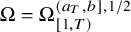 $\Omega =\Omega _{[1,T)}^{(a_T,b],1/2}$
. Then
 $$\begin{align*}L(\underline{x};b)\cap [1,T) = L(\underline{x};a_{T})\cap [1,T) \bigsqcup Q_\Omega(\underline{x}). \end{align*}$$
By Lemma 11.1,
 $L(\underline {x};a_{T}) = \emptyset $
for all almost all
 $\underline {x} \in \mathbb {R}^2$
and sufficiently large T (depending on
 $\underline {x}$
), and thus
 $L(\underline {x};b)\cap [1,T) = Q_\Omega (\underline {x})$
. Hence, Theorem 1.1 follows from Theorem 1.2 and the volume formula (A.4).
A Volume estimates
In this section we discuss some basic facts concerning the volumes of the sets
 $$\begin{align*}\Omega = \left\{ (\underline{x},y) \in \mathbb{R}^2 \times [1,T) \, : \, \begin{array}{c} \max(|x_1|,|x_2|) \leq c \\[0.2cm] a < |x_1x_2| \cdot y \leq b \end{array} \right\} \end{align*}$$
with
 $0<a<b< 1$
and
 $c\le 1/2$
. We observe that these domains can be represented in terms of more basic sets

Direct computation gives
 $$ \begin{align} \operatorname{\mathrm{Vol}}_2(\Xi(\gamma)) = 4\max\big(1,\gamma \cdot (1 - \ln\gamma)\big)\quad \text{for } \gamma>0. \end{align} $$
In particular, it follows from the Mean Value Theorem that
 $$ \begin{align} \operatorname{\mathrm{Vol}}_2(\Xi(\gamma_2))-\operatorname{\mathrm{Vol}}_2(\Xi(\gamma_1))\le 4|\ln\min(1,\gamma_1)|\cdot (\gamma_2-\gamma_1) \quad \text{for } \gamma_2>\gamma_1>0. \end{align} $$
We observe that the y-sections
 $$\begin{align*}\Omega(y) := \{ \underline{x} \in \mathbb{R}^2 \, : \, (\underline{x},y) \in \Omega \}, \quad \text{for } y \in [1,T). \end{align*}$$
can be written as
 $$\begin{align*}\Omega(y) = c\cdot\left(\Xi\left( \frac{b}{c^2 \cdot y}\right) \setminus \Xi\left(\frac{a}{c^2 \cdot y}\right)\right), \end{align*}$$
and thus
 $$\begin{align*}\operatorname{\mathrm{Vol}}_2(\Omega(y)) = c^2 \cdot \left( \operatorname{\mathrm{Vol}}_2\left(\Xi\left( \frac{b}{c^2 \cdot y}\right)\right)-\operatorname{\mathrm{Vol}}_2\left(\Xi\left( \frac{a}{c^2 \cdot y}\right)\right)\right), \quad \text{for all } y \in [1,T). \end{align*}$$
In view of this, the following lemma can be deduced from (A.2) by a direct computation:
Lemma A.1. For
 $\max (1,\frac {b}{c^{2}}) \leq y < T$
,
 $$ \begin{align*} \operatorname{\mathrm{Vol}}_2(\Omega(y)) =\ & \frac{4 \cdot \ln y}{y} \cdot (b-a) \\ & + \frac{4}{y} \cdot \Big( (b-a) \cdot (1 + 2 \cdot \ln c) - b \ln b + a \ln a \Big), \end{align*} $$
so that when
 $b\ll c^2$
,
 $$ \begin{align*} \operatorname{\mathrm{Vol}}_3(\Omega) =\ & 2 \cdot (\ln T)^2 \cdot (b-a) \\ &+ 4 \cdot \ln T \cdot \Big( (b-a) \cdot (1 + 2 \cdot \ln c) - b \ln b + a \ln a \Big)+O(1). \end{align*} $$
In particular, if in addition
 $a \gg (\ln T)^{-\theta }$
for some
 $\theta> 0$
, then
 $$ \begin{align} \operatorname{\mathrm{Vol}}_3(\Omega) = 2 \cdot (\ln T)^2 \cdot (b - a) + O\Big(\ln T(\ln\ln T)\cdot(b-a)+1\Big). \end{align} $$
B An auxiliary double sum
This is a largely technical section where we collect some estimates on certain multiparameter sums that are used in Section 7. This part can be safely skipped on a first read.
We begin with a simple observation. For
 $\underline {u} = (u_1,u_2) \in \mathbb {R}^2_{+}$
, let

A simple counting argument that we leave to the reader shows that
 $N(\underline {u}) \ll G(\underline {u})$
, where
 $$ \begin{align} G(\underline{u}) = \left\{ \begin{array}{cl} 1 & \text{if } \lceil \underline{u} \rceil < 1 \\[0.2cm] \lceil \underline{u} \rceil & \text{if } \lfloor \underline{u} \rfloor < 1 \leq \lceil \underline{u} \rceil \\[0.2cm] u_1 u_2 & \text{if } 1 \leq \lfloor \underline{u} \rfloor \end{array} \right.. \end{align} $$
Let us fix a constant
 $M> 0$
for the rest of the section. For
 $t = (t_1,t_2) \in \mathbb {R}^{2}_{+}$
, we define the function
 $$ \begin{align} F_t(q) = \frac{G(2Mqe^{-t_1},2Mqe^{-t_2})}{q^2} \cdot e^{-(t_1 + t_2)}, \quad q \geq 1. \end{align} $$
The explicit formula for G above tells us that
 $$ \begin{align} F_t(q) = \left\{ \begin{array}{cl} \frac{e^{-(t_1 + t_2)}}{q^2} & \text{if } q < \frac{e^{\lfloor t \rfloor}}{2M} \\[0.2cm] 2M\frac{e^{-(2\lfloor t \rfloor + \lceil t \rceil)}}{q} & \text{if } \frac{e^{\lfloor t \rfloor}}{2M} \leq q < \frac{e^{\lceil t \rceil}}{2M} \\[0.2cm] 4M^{2}e^{-2(t_1 + t_2)} & \text{if } \frac{e^{\lceil t \rceil}}{2M} \leq q \end{array} \right.. \end{align} $$
Our main goal in this section is to prove the following upper bound on an auxiliary double sum which involves the function
 $F_t$
.
Lemma B.1. Let
 $0 < \alpha < \beta \leq M$
and let
 $t = (t_1,t_2) \in \mathbb {R}^2_{+}$
. Define
 $$\begin{align*}\alpha_t = \alpha \cdot e^{t_1 + t_2} \quad \text{and} \quad \beta_t = \beta \cdot e^{t_1 + t_2} \end{align*}$$
and suppose that
 $\alpha <1$
,
 $\alpha _t \geq 1$
. Then,
 $$\begin{align*}\sum_{q_1, q_2 = \alpha_t}^{\beta_t} F_t\left( \frac{\max(q_1,q_2)}{\gcd(q_1,q_2)}\right) \ll_M e^{-(t_1+t_2)} + (\beta-\alpha) \cdot \max\left(1,\ln\left(\frac{\beta}{\alpha}\right)\right) \cdot \max(1,t_1 + t_2), \end{align*}$$
where the implicit constants depend only on M.
Remark B.2. We adopt the following sum convention: If
 $1 \leq \gamma < \delta $
, and m and n are integers such that
 $$\begin{align*}m < \gamma \leq m+1 \quad \text{and} \quad n \leq \delta < n+1, \end{align*}$$
then
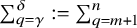 $\sum _{q = \gamma }^\delta := \sum _{q = m+1}^n$
, where the right-hand side is defined to be zero if
 $m = n$
.
B.1 Proof of Lemma B.1
The following standard estimates will be used in the proof. For
 $1 \leq \gamma < \gamma +1 <\delta $
we have
 $$ \begin{align} \sum_{q = \gamma}^\delta \frac{1}{q} &=\ln\left(\frac{\delta}{\gamma}\right)+\mathcal{O}\left(\frac{1}{\gamma}\right), \end{align} $$
where the implicit constants are independent of
 $\gamma $
and
 $\delta $
. In addition, the following elementary upper bound on the sum-of-divisors function holds
 $$ \begin{align} \frac{1}{n} \sum_{\substack{m=1 \\ m \mid n}}^{n} m \ll \ln(n). \end{align} $$
Let us begin with the proof. We fix
 $t = (t_1,t_2) \in \mathbb {R}^2_{+}$
and
 $0 < \alpha < \beta \leq M$
such that
 $$\begin{align*}1> \alpha \quad \text{and} \quad \alpha_t \geq 1 \quad \text{and} \quad e^{\lfloor t \rfloor} > 2M, \end{align*}$$
and we want to bound the double sum
 $$\begin{align*}S_t(\alpha,\beta) := \sum_{q_1, q_2 = \alpha_t}^{\beta_t} F_t\left( \frac{\max(q_1,q_2)}{\gcd(q_1,q_2)} \right) \end{align*}$$
from above. Note that
 $F_t(1)\ll _{M} e^{-(t_1 + t_2)}$
.
We first consider the case when
 $\beta _t - \alpha _t < 1$
. Then, the double sum above contains at most one term (necessarily with
 $q_1 = q_2$
), and thus
 $$ \begin{align} S_t(\alpha,\beta) \leq F_t(1) \ll_M e^{-(t_1 + t_2)}. \end{align} $$
Let us from now on assume that
 $\beta _t - \alpha _t \geq 1$
, and define the sets
 $$ \begin{align*} \mathcal{E}_0 &:= \left\{ (q_1,q_2) \in [\alpha_t,\beta_t]^2 \cap \mathbb{N}^2 \, : \, \frac{\max(q_1,q_2)}{\gcd(q_1,q_2)} < \frac{e^{\lfloor t \rfloor}}{2M} \right\}, \\[0.2cm] \mathcal{E}_1 &:= \left\{ (q_1,q_2) \in [\alpha_t,\beta_t]^2 \cap \mathbb{N}^2 \, : \, \frac{e^{\lfloor t \rfloor}}{2M} \leq \frac{\max(q_1,q_2)}{\gcd(q_1,q_2)} < \frac{e^{\lceil t \rceil}}{2M} \right\}, \\[0.2cm] \mathcal{E}_2 &:= \left\{ (q_1,q_2) \in [\alpha_t,\beta_t]^2 \cap \mathbb{N}^2 \, : \, \frac{e^{\lceil t \rceil}}{2M} \leq \frac{\max(q_1,q_2)}{\gcd(q_1,q_2)} \right\}, \end{align*} $$
and the functions
 $$\begin{align*}S_t^{(k)}(\alpha,\beta) := \sum_{(q_1,q_2) \in \mathcal{E}_k} F_t\left(\frac{\max(q_1,q_2)}{\gcd(q_1,q_2)} \right), \quad \text{for } k=0,1,2. \end{align*}$$
Note that
 $$\begin{align*}S_t(\alpha,\beta) = S_t^{(0)}(\alpha,\beta) + S_t^{(1)}(\alpha,\beta) + S_t^{(2)}(\alpha,\beta). \end{align*}$$
We will estimate these three partial sums separately below.
An upper bound for
$S_t^{(0)}(\alpha ,\beta )$

Note that if
 $\gcd (q_1,q_2) = d$
, then
 $$\begin{align*}\left(\frac{\gcd(q_1,q_2)}{\max(q_1,q_2)}\right)^2 = \frac{d^2}{\max(q_1,q_2)^2} \leq \frac{d}{q_1 \cdot q_2'}, \end{align*}$$
where
 $q_2 = d \cdot q_2'$
. Hence,
 $$ \begin{align*} S_t^{(0)}(\alpha,\beta) &= \sum_{(q_1,q_2) \in \mathcal{E}_o} \left(\frac{\gcd(q_1,q_2)}{\max(q_1,q_2)}\right)^2 \cdot e^{-(t_1 + t_2)} \leq \sum_{q_1,q_2 = \alpha_t}^{\beta_t} \left(\frac{\gcd(q_1,q_2)}{\max(q_1,q_2)}\right)^2 \cdot e^{-(t_1 + t_2)} \\[0.2cm] &\leq 2 \cdot \sum_{q_1 = \alpha_t}^{\beta_t} \left( \sum_{\substack{d=1 \\ d \mid q_1}}^{q_1} \, \sum_{q_2' = \frac{\alpha_t}{d}}^{\frac{\beta_t}{d}} \frac{d}{q_1 \cdot q_2'} \right) \cdot e^{-(t_1 + t_2)}. \end{align*} $$
By (B.5) (with
 $\gamma = \frac {\alpha _t}{d}$
and
 $\delta = \frac {\beta _t}{d}$
), we now see that
 $$ \begin{align*} S_t^{(0)}(\alpha,\beta) &\ll \sum_{q_1 = \alpha_t}^{\beta_t} \left( \frac{1}{q_1} \sum_{\substack{q_1 = 1 \\ d \mid q}}^{q_1} d \right) \cdot \left( 1 + \ln\left(\frac{\beta}{\alpha}\right) \right) \cdot e^{-(t_1 + t_2)}, \end{align*} $$
and by (B.6),
 $$ \begin{align*} \sum_{q = \alpha_t}^{\beta_t} \left( \frac{1}{q} \sum_{\substack{q = 1 \\ d \mid q}} d \right) \cdot e^{-(t_1 + t_2)} &\ll \left( \sum_{q=\alpha_t}^{\beta_t} \ln(q) \right) \cdot e^{-(t_1 + t_2)} \leq (\beta_t - \alpha_t) \cdot \ln(\beta_t) \cdot e^{-(t_1 + t_2)} \\[0.2cm] &\ll_M (\beta-\alpha) \cdot \max(1,t_1 + t_2), \end{align*} $$
since
 $\beta \leq M$
. We conclude that
 $$ \begin{align} S_t^{(0)}(\alpha,\beta) \ll (\beta-\alpha) \cdot \max\left(1,\ln\left(\frac{\beta}{\alpha}\right)\right) \cdot \max(1,t_1 + t_2). \end{align} $$
An upper bound for
$S_t^{(1)}(\alpha ,\beta )$

To simplify notation, let us assume that
 $t_1 \leq t_2$
so that
 $\lfloor t \rfloor = t_1$
and
 $\lceil t \rceil = t_2$
. Then,
 $$\begin{align*}S_t^{(1)}(\alpha,\beta) = \left( \sum_{(q_1,q_2) \in \mathcal{E}_1} \frac{\gcd(q_1,q_2)}{\max(q_1,q_2)} \right) \cdot e^{-(2t_1 + t_2)}, \end{align*}$$
If
 $(q_1,q_2) \in \mathcal {E}_1$
, then
 $$\begin{align*}\frac{e^{t_1}}{2M} \leq \frac{\max(q_1,q_2)}{\gcd(q_1,q_2)} \quad \text{and} \quad \max(q_1,q_2) \leq \beta_t = \beta \cdot e^{t_1 + t_2}, \end{align*}$$
and thus
 $\gcd (q_1,q_2) \leq 2M \cdot \beta \cdot e^{t_2}$
. Let
 $\gamma _t = \min (\alpha _t,2M \cdot \beta \cdot e^{t_2})$
, and note that
 $$ \begin{align*} S_t^{(1)}(\alpha,\beta) &\leq \sum_{d=1}^{\gamma_t} \left( \sum_{q_1,q_2 = \frac{\alpha_t}{d}}^{\frac{\beta_t}{d}} \frac{1}{\max(q_1,q_2)} \right) \cdot e^{-(2t_1 + t_2)} \\[0.2cm] &\quad+ \sum_{d=\alpha_t}^{\beta_t} \left( \sum_{q_1,q_2 = 1}^{\frac{\beta_t}{d}} \frac{1}{\max(q_1,q_2)} \right) \cdot e^{-(2t_1 + t_2)} \\[0.2cm] &\ll \left( \sum_{d=1}^{\gamma_t} \frac{\beta_t - \alpha_t}{d} \right) \cdot e^{-(2t_1 + t_2)} + \left( \sum_{d=\alpha_t}^{\beta_t} \frac{\beta_t}{d} \right) \cdot e^{-(2t_1 + t_2)} \\[0.2cm] &\ll (\beta-\alpha) \cdot (1 + \ln(\gamma_t)) \cdot e^{-t_1} + \beta \cdot \left(\ln\left(\frac{\beta}{\alpha}\right)+\mathcal{O}\left(\frac{1}{\alpha_{t}}\right) \right) \cdot e^{-t_1}, \end{align*} $$
where we in the last inequality have used (B.5) (with parameters
 $\gamma = 1, \delta = \gamma _t$
and
 $\gamma = \alpha _t, \delta = \beta _t$
). Since
 $$\begin{align*}\ln(\gamma_t) \ll 1 + t_2, \end{align*}$$
we have
 $$ \begin{align*}(\beta-\alpha) \cdot (1 + \ln(\gamma_t)) \cdot e^{-t_1}\ll_{M}(\beta-\alpha) \cdot \max(1,t_1 + t_2) \cdot e^{-\lfloor t \rfloor}.\end{align*} $$
For the term
 $$ \begin{align*}\beta \cdot \left(\ln\left(\frac{\beta}{\alpha}\right)+\mathcal{O}\left(\frac{1}{\alpha_{t}}\right) \right) \cdot e^{-t_1},\end{align*} $$
we consider two separate cases. If
 $\beta /\alpha \geq e$
, then
 $\ln (\beta /\alpha )$
dominates, and since
 $\beta -\alpha \gg \beta $
, we find
 $$ \begin{align*}\beta \cdot \left(\ln\left(\frac{\beta}{\alpha}\right)+\mathcal{O}\left(\frac{1}{\alpha_{t}}\right) \right) \cdot e^{-t_1}\ll_{M}(\beta-\alpha)\cdot\ln\left(\frac{\beta}{\alpha}\right)\cdot e^{-t_{1}}.\end{align*} $$
If
 $\beta /\alpha <e$
, on the other hand, we deduce
 $$ \begin{align*}\beta \cdot \left(\ln\left(\frac{\beta}{\alpha}\right)+\mathcal{O}\left(\frac{1}{\alpha_{t}}\right) \right) \cdot e^{-t_1}\ll_{M}\beta\cdot\ln\left(\frac{\beta}{\alpha}\right)\cdot e^{-t_{1}}+\frac{\beta}{\alpha}\cdot e^{-2t_{1}-t_{2}}.\end{align*} $$
On observing that for
 $1<\beta /\alpha \leq e$
 $$ \begin{align*}\beta\cdot \ln\left(\frac{\beta}{\alpha}\right)\ll(\beta-\alpha),\end{align*} $$
we now obtain
 $$ \begin{align*}\beta \cdot \left(\ln\left(\frac{\beta}{\alpha}\right)+\mathcal{O}\left(\frac{1}{\alpha_{t}}\right) \right) \cdot e^{-t_1}\ll_{M}(\beta-\alpha)\cdot e^{-t_{1}}+e^{-2t_{1}-t_{2}}.\end{align*} $$
Then, by combining the previous estimates, we conclude that
 $$ \begin{align} S_t^{(1)}(\alpha,\beta) \ll_M (\beta-\alpha) \cdot \max\left(1,\ln\left(\frac{\beta}{\alpha}\right)\right) \cdot \max(1,t_1 + t_2) \cdot e^{-\lfloor t \rfloor}+e^{-(t_{1}+t_{2})}. \end{align} $$
An upper bound for
$S_t^{(2)}(\alpha ,\beta )$

The following crude estimate will suffice:
 $$ \begin{align} S^{(2)}_t(\alpha,\beta) &= \left( \sum_{(q_1,q_2) \in \mathcal{E}_2} 1 \right) \cdot e^{-2(t_1 + t_2)} \leq \left( \sum_{q_1=\alpha_t}^{\beta_t} \sum_{q_2 = \alpha_t}^{\beta_t} 1\right) \cdot e^{-2(t_1 + t_2)} \nonumber \\[0.2cm] &\ll (\beta_t-\alpha_t)^2 \cdot e^{-2(t_1 + t_2)} \ll_M (\beta-\alpha)^2 \ll \beta-\alpha, \end{align} $$
since
 $\beta \leq M$
.
Putting it all together
If we now combine (B.7), (B.8), (B.9) and (B.10), we get
 $$\begin{align*}S_t(\alpha,\beta) \ll_M e^{-(t_1+t_2)} + (\beta-\alpha) \cdot \max\left(1,\ln\left(\frac{\beta}{\alpha}\right)\right) \cdot \max(1,t_1 + t_2), \end{align*}$$
where the implicit constants are independent of
 $\alpha $
and
 $\beta $
, and hence the proof of Lemma B.1 is complete.
Acknowledgements
We would like to thank Shunsuke Usuki for pointing out issues in a previous version of the paper.
Competing interests
The authors have no competing interest to declare.

 Open access

