2.1. Wind tunnel and flat-plate model

Experiments are conducted in a low-speed closed-loop wind tunnel at the National Key Lab of Aerospace Power System and Plasma Technology. The free-stream velocity of the wind tunnel ( $U_\infty$ ) can be adjusted from 3 to 40 m s⁻¹, with a typical turbulence intensity of less than 0.2 %. In the middle of the rectangular test section (height: 1 m; width: 1.2 m), a flat-plate model made of Plexiglas is mounted horizontally. This plate has an elliptical leading edge and a wedge-shaped trailing edge (figure 1), such that a zero-pressure-gradient boundary layer can develop smoothly on the upper surface of the model. At 50 mm downstream of the plate leading edge, a transition tape made of sandpaper (width: 40 mm) is pasted to trip the incoming boundary layer into turbulent state. A plasma actuator array is flush-mounted in the downstream half of the plate, and the distance between the actuator and plate leading edge is 1140 mm. The streamwise and spanwise extents of the plasma actuator are 120 mm. At the upstream end of the fifth exposed electrode, a coordinate system is established, with the $x$ , $y$ and $z$ axes aligned with the streamwise, wall-normal and spanwise directions, respectively (figure 1 $b$ ). In this study, the free-stream velocity is set as $U_\infty = 20$ m s⁻¹, yielding a boundary-layer thickness of $\delta _{99} = 22.1$ mm at a streamwise station of $x = 50$ mm.

Figure 1.

Sketch of ( $a$ ) the flat-plate model and ( $b$ ) a cross-sectional view of the plasma actuator. Not to scale.

2.2. Actuators and sensors

2.2.1. Plasma actuators

For the purpose of turbulent drag reduction, various configurations of dielectric barrier discharge plasma actuators have been proposed, such as the unidirectional spanwise plasma jet actuator array (Duong, Corke & Thomas Reference Duong, Corke and Thomas2020), streamwise plasma jet actuator array (Wu et al. Reference Wu, Gao, Liu, Xue, Wang and Zheng2019) and spanwise oscillating plasma jet actuator array (Hehner et al. Reference Hehner, Gatti, Mattern, Kotsonis and Kriegseis2020). In the present study, a spanwise impinging plasma jet actuator array is employed for control. Such a geometrical configuration is expected to produce large-scale streamwise vortices (LSSVs) that suppresses the turbulent streak instability. The prospect of such a spanwise forcing in friction-drag reduction has been demonstrated in both early DNS (Schoppa & Hussain Reference Schoppa and Hussain1998; Canton et al. Reference Canton, Örlü, Chin, Hutchins, Monty and Schlatter2016; Yao et al. Reference Yao, Chen, Thomas and Hussain2017, Reference Yao, Chen and Hussain2018) and recent wind tunnel tests (Cheng et al. Reference Cheng, Wong, Hussain, Schröder and Zhou2021; Wei & Zhou Reference Wei and Zhou2025).

In total, nine actuator units are arranged spanwise in the array, with a centre-to-centre spacing of $L$ = 10 mm (540 $\delta _\nu$ ) close to that of the turbulent streak spacing (415 $\delta _\nu$ ). Figure 1( $b$ ) shows a cross-sectional view of the plasma actuator, consisting of high-voltage electrodes, ground electrodes and a dielectric layer. In the two lateral sides of the ground electrode (width: 9 mm; thickness: 45 μm), two high-voltage electrodes (width: 1 mm; thickness: 45 μm) are arranged, such that a pair of opposing wall jets are induced by electrostatic forces. As with the material of the dielectric layer (thickness: 0.35 mm), we choose a special composite called RO4350B. Compared with the widely adopted Kapton dielectric layer (Corke et al. Reference Corke, Enloe and Wilkinson2010), inorganic additives are mixed in RO4350B, making it more resistant to plasma corrosion. Consequently, the plasma actuator can work stably for weeks, eliminating the inconsistency of drag-reduction results introduced by actuator degradation. The dielectric layer’s dimensions (120 mm $\times$ 120 mm) are intentionally designed to be larger than the plasma discharge zone (100 mm $\times$ 100 mm) to ensure that the minor gap at the dielectric layer edges does not interfere with boundary-layer development in the measurement zone.

Figure 2.

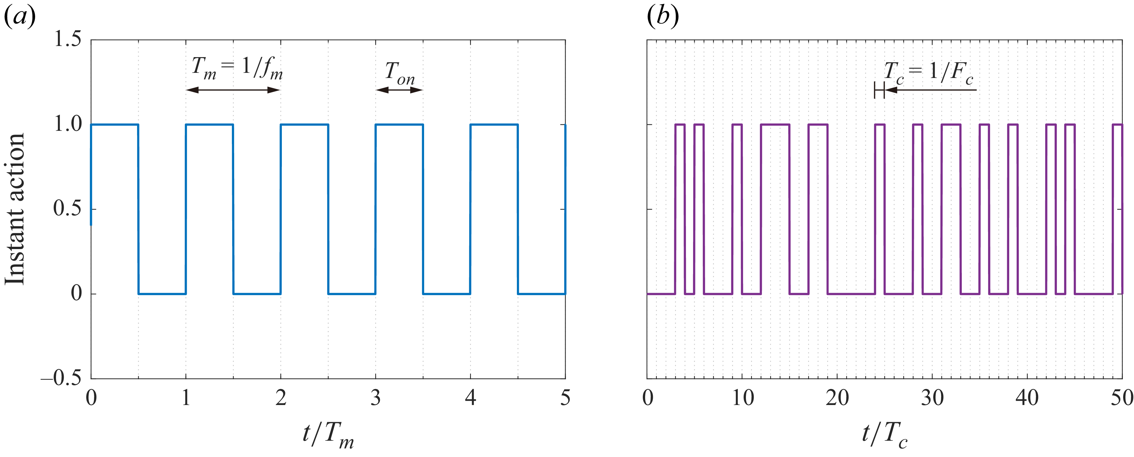
Sketch of the action signals in ( $a$ ) open-loop periodical control ( $f_m$ = 100 Hz) and ( $b$ ) on-demand DRL control ( $F_c$ = 1000 Hz).

For the purpose of on-demand real-time adjustment of the plasma jet strength, a high-voltage sinusoidal power supply (Coronalab, CTP-2000K) together with a programmable alternating-current power source (IVYTECH, APS50001A) are employed to drive the plasma actuator. The output voltage waveform can be conveniently regulated by a serial port and an enable signal. For optimal impedance match between the power supply and the actuator, the base frequency of the sinusoidal waveform ( $f_b$ ) is fixed at 10 kHz. Discharge waveforms of the plasma actuator are measured by a voltage probe (Tektronix, P6015A) and a current probe (Tektronix, P6022), based on which the actuator power consumption can be calculated. Figure 2 compares the representative action signals in open-loop and DRL control. For the open-loop control strategy, periodical actuation with a modulated sinusoidal waveform is imposed to the plasma actuator, leaving three influential parameters to be tuned, namely the voltage amplitude ( $U_a$ ), modulation frequency ( $f_m$ ) and duty cycle ( $D_c$ ). By definition, we have $D_c= T_{\textit{on}}/T_m$ , where $T_{\textit{on}}$ and $T_m$ denote, respectively, the discharge duration and the modulation period ( $T_m=1/f_m$ ). As a comparison, in DRL control, a logic command is computed from the neural network which then determines the ‘ON/OFF’ status of the plasma actuator within one control period ( $T_c$ ). The control frequency ( $F_c$ ) is related to the control period by $F_c=1/T_c$ .

2.2.2. Shear stress sensors

Many friction-drag measurement devices have been proposed in the literature, such as the floating balance (Cheng et al. Reference Cheng, Wong, Hussain, Schröder and Zhou2021), total pressure probes (Sutardi & Ching Reference Ching2001), micro-PIV (Kähler et al. Reference Kähler, Scholz and Ortmanns2006), laser Doppler velocimetry (Mazumder et al. Reference Mazumder, Wanchoo, McLeod, Ballard, Mozumdar and Caraballo1981), microelectromechanical system sensors (Zhe, Modi & Farmer Reference Zhe, Modi and Farmer2005) and oil-film techniques (Örlü & Vinuesa Reference Örlü and Vinuesa2020). However, most of these devices have a low frequency response and complex data processing, unsuitable for real-time closed-loop control that requires instantaneous skin-friction drag evaluation. Consequently, thermal-based hot films and wall hot wires are chosen as the senors. These devices offer high-frequency bandwidth up to 10 kHz and produce analogue electrical signals that can be processed directly by the controller.

Ideally, since the boundary-layer states at different spanwise positions of the actuator zone can differ, each plasma actuator unit should be driven independently, acting based on its own upstream sensor signal. However, practical implementation of such a distributed DRL control system faces substantial challenges. Not only is significant hardware required, but also destructive cross-anode discharge can arise from the asynchronous variation of voltage. Therefore, the present study focuses on only the middle plasma actuator unit, and the control objective is set to minimise the drag downstream of it. Similar practice can be found in Wong et al. (Reference Wong, Cheng, Fan, Li and Zhou2021). As depicted in figure 1( $a$ ), two hot-film sensors (Dantec, 55R47) and two wall hot-wire sensors (ChangZhou Turbulence Technology, HF-1) are configured upstream ( $x/L = -1.65$ ) and downstream ( $x/L = 12$ ) of the actuator zone to measure the time-resolved local wall shear stress. In the DRL framework, these sensors serve distinct roles: the upstream sensors provide state information of the incoming TBL, while the downstream sensors evaluate the control consequence (reward). Wall hot wires were employed instead of hot films as the downstream wall shear stress evaluators, due to the rapid performance degradation observed in the hot-film material when installed downstream of the plasma zone. Usage of the wall hot wire as a shear stress sensor can also be found in the closed-loop drag-reduction control experiment in Yu et al. (Reference Yu, Fan, Noack and Zhou2021). Structurally, as shown in the insets in figure 1( $a$ ), the specially designed wall hot wire takes a cylindrical body (diameter: 3 mm), and the distance from the wire to the wall is only 0.2 mm, corresponding to a height of $y^+ \approx 11$ in wall units, comparable to the sensor setting in Rebbeck & Choi (Reference Rebbeck and Choi2001) ( $y^+ = 8$ ) and Choi et al. (Reference Choi, Moin and Kim1994) ( $y^+ = 10$ ) for opposition control of turbulence.

The two hot-film sensors, located at $[x/L,\; z/L]=[-1.65,\;-1]$ and $[x/L,\; z/L]=[-1.65,\;0]$ , are referred to as HF1 and HF2 hereinafter. Similarly, the two hot-wire sensors, situated at $[x/L,\; z/L]=[12,\;-0.5]$ and $[x/L,\; z/L]=[12,\;0]$ , are labelled as HW1 and HW2. Along the streamwise direction, both HF1 and HF2 are aligned with the high-voltage electrodes, with a dimensionless spanwise spacing of 540 wall units. As a comparison, the spanwise spacing between the downstream hot wires is designed to be 0.5 $L$ ( $270 \delta _\nu$ ), such that HW1 and HW2 are located, respectively, at the downwash and upwash zones of the plasma actuation, and the mean value of their outputs can somehow reflect the spanwise-averaged wall shear stress downstream (Zong et al. Reference Zong, Su, Liang and Wu2022; Benard, Bonnet & Moreau Reference Benard, Bonnet and Moreau2024; Fang et al. Reference Fang, Zong, Zhang, Wu, Su, Liang and Bian2024). In Wong et al. (Reference Wong, Cheng, Fan, Li and Zhou2021), similar impinging plasma jets were used to actuate the TBL, and the spanwise distribution of skin-friction drag was diagnosed in detail. According to their results, the spanwise extent of the drag-reduction zone is much larger than that of the drag-increase zone, and using the mean value of the two hot-wire measurements as an estimate approximately leads to an underestimation of the spanwise-averaged drag reduction by approximately 4.4 %.

Figure 3.

Calibration curves of the hot wires and hot films.

All of the four sensors are driven by a constant-temperature anemometer (Hanghua CTA-04 Pro). To obtain the calibration curves, the baseline wall shear stresses (denoted as $\tau _{bl}$ ) at increasing free-stream velocity ( $U_\infty$ ) are first assessed with PIV measurements, by following the procedure described in § 2.4. Then, the output voltages of the four sensors (denoted as $V_{\textit{sen}}$ ) at known wall shear stresses are recorded. Finally, for each sensor, by fitting the relationship between $V_{\textit{sen}}$ and $\tau _{bl}$ as a fourth-order polynomial (Lekakis Reference Lekakis1996), the corresponding calibration curve can be derived. As shown in figure 3, the calibration curves can effectively reproduce the variation trends of $V_{\textit{sen}}$ . Particularly, in the range of $0.2\leqslant \tau _{bl}\leqslant 1$ , the sensor voltages increase approximately linearly with the wall shear stress. Using these calibration curves, the flow states of the upstream and downstream boundary layers can be readily evaluated.

2.3. The DRL control framework

In addition to the actuators and sensors, the controller represents another crucial hardware component in a closed-loop flow control system. A compact real-time controller (National Instruments, cRIO-9049) with an embedded FPGA chip is deployed to implement the DRL control. In the chassis of this controller, an analogue input module (NI-9205) and an analogue output module (NI-9264) are mounted for acquiring the sensor signals and transmitting the control commands, respectively. Since our task is a discrete control task, a classical value-based DRL algorithm, deep Q-network (DQN), is adopted.

Figure 4.

Data and work flow in the FPGA-based experimental DRL control framework.

Figure 4 sketches the basic data and work flows in DQN, which is adapted from the original FPGA-based experimental DRL (FeDRL) control framework proposed by Zong et al. (Reference Zong, Wu, Li, Su and Liang2025). Compared with the traditional CPU-based DRL control framework which has a typical control frequency of 10–100 Hz (Shimomura et al. Reference Shimomura, Sekimoto, Oyama, Fujii and Nishida2020), the FeDRL reduces the control latency to $O$ (100 μs), enabling real-time execution of a neural network control law at 1–10 kHz. The FeDRL framework includes a high-speed real-time control loop and a slow network training loop. In each control loop, the FPGA first acquires the instantaneous voltage signals from HF1 and HF2 (denoted as $v^1_{h,t}$ and $v^2_{h,t}$ ). These signals are then normalised using their respective baseline statistics to form a dimensionless flow state vector ${\boldsymbol{s}}_{\kern-1pt\boldsymbol{t}}$ :

(2.1) \begin{equation} \left \lbrace \begin{array}{ll} \displaystyle s_t^i=\frac {v^i_{h,t}-\bar {v}^i_{h,bl}}{\tilde {v}^i_{h,bl}}, \hspace{10pt} \textrm{for}\quad i=[1,2] \\[16pt] {\boldsymbol{s}}_{\kern-1pt\boldsymbol{t}}= \left[s_t^1, s_t^2 \right], \end{array} \right . \end{equation}

where variables with a bar and a tilde represent the mean value and standard deviation under non-actuated condition, respectively. Assuming the raw voltages of the hot films follow roughly a Gaussian distribution, $s_t^1$ and $s_t^2$ would have a typical range of −3 to 3.

Previous studies have shown that by incorporating past sensor signals into the state feature vector of the environment, the robustness of DRL can be improved (Wang et al. Reference Wang, Yan, Hu, Chen, Rabault and Noack2024). Inspired by this, a first-in first-out (FIFO) sequence is built in the FPGA to host the history states, called S-FIFO. Assuming the number of input nodes in the Q-network is $N_s$ , the network input vector is defined based on the normalised state values as follows:

(2.2) \begin{equation} \displaystyle {\boldsymbol{x}}_{\boldsymbol{t}}=[{\boldsymbol{s}}_{\kern-1pt\boldsymbol{t}}, \boldsymbol{s_{{\kern-1pt}t-1}}, \ldots , \boldsymbol{s_{{\kern-1pt}t-N_s/2+1}}]= \Big[s_t^1, s_t^2, s_{t-1}^1, s_{t-1}^2, \ldots , s_{t-N_s/2+1}^1, s_{t-N_s/2+1}^2 \Big], \end{equation}

where $N_s$ is an even number.

In DQN, the value function is commonly parametrised by a fully connected neural network. For real-time closed-loop control, to effectively improve the network training efficiency and inference speed, a radial basis function (RBF) neural network is preferred, which remains a universal function approximator but incorporates many fewer parameters. The RBF network outputs two Qvalues ( $Q_1$ and $Q_2$ ), corresponding to the long-term reward expected to be received by the agent after the plasma actuator takes an ON/OFF action (denoted as $a_t$ : 0 or 1). Mathematically, the Q-function represented by the RBF network can be written in the following form:

(2.3) \begin{equation} \left \lbrace \begin{array}{l} \mathbf{Q_{2\times 1}}=\mathbf{W_{2\times m}}\boldsymbol{\cdot }\left [ \phi _1(\textbf{x}),\phi _2(\textbf{x}),\ldots ,\phi _m(\textbf{x})\right ]^{\textbf{T}}+\mathbf{B_{2\times 1}} \\ \phi _i=\textrm{exp}(-h_i\left |\left |\textbf{x}-\mathbf{c_i}\right |\right |^2), \hspace{10pt} \textrm{for}\; \; i=[1,2,\ldots ,m], \end{array} \right . \end{equation}

where $\phi _i$ is the Gaussian kernel function and $h_i$ and ${\boldsymbol{c}}_{\boldsymbol{i}}$ represent the variance and centre of $\phi _i$ . The weights connecting the hidden layer to the output layer and the biases of the output layer are denoted by $\mathbf{W_{2\times m}}$ and $\mathbf{B_{2\times 1}}$ , respectively.

To ensure proper and stable learning, an instant reward ( $r_t$ ) is provided to the agent. This reward reflects the ensemble-averaged influence of the plasma actuator on the skin-friction drag. The reward signal is derived from the instantaneous signals of HW1 and HW2, denoted as $v_{w,t}^1$ and $v_{w,t}^2$ , following the reward shaping scheme of Chen et al. (Reference Chen, Zong, Song, Wu, Liang and Xiang2024b ):

(2.4) \begin{equation} \left \lbrace \begin{array}{ll} \displaystyle \mu _t^i=\frac {v^i_{w,t}-\bar {v}^i_{w,bl}}{\tilde {v}^i_{w,bl}}, \hspace{10pt} \textrm{for}\;\;i=[1,2]\\[12pt] r_t=\displaystyle {-\frac {1}{2R_l}\sum _{j= 1}^{j=R_l} \Big(\mu _{t-R_d+j}^1+\mu _{t-R_d+j}^2 \Big)}, \end{array} \right . \end{equation}

where $\mu _t^i$ is the dimensionless hot-wire voltage normalised by the statistics obtained under non-actuated condition, analogous to the first operation in (2.1); $R_d$ and $R_l$ dictate the reward time delay and the reward smoothing length, respectively, both of which are in units of control periods.

Essentially, the instant reward is defined as the negative of the sliding-averaged value of $\mu _t^i$ in a time-delay window. The negation operator is easily understandable, since our objective is to reduce the overall friction drag, and a negative dimensionless voltage indicates a low shear stress which should be rewarded positively. Addition of the time delay is due to the fact that boundary-layer flow is a strongly convective flow, and the downstream sensors need some time to feel the changes caused by the upstream plasma actuation. Such a time delay can be roughly estimated by $x_{hw}/U_{y^+=11}\approx 14$ ms, where $x_{hw}$ is the streamwise distance between the hot film and wall hot wire. The sliding-averaging operation is intended to reduce the measurement uncertainty and improve the learning stability, as has been demonstrated by Chen et al. (Reference Chen, Zong, Song, Wu, Liang and Xiang2024b ). After the above procedure, we eventually get a piece of control experience: $[\boldsymbol{x}_{{\kern-1pt}t}, a_t, r_t, \boldsymbol{x}_{{\kern-1pt}t+1}]$ . This experience is subsequently inserted into a FIFO sequence, called E-FIFO.

In the learning loop (refer to the right-hand panel of figure 4), a LabVIEW program is built in the host computer, serving as a communication bridge between the Python (trainer) and the FPGA (executor). Experience data stored in the E-FIFO of the FPGA are first transmitted to the LabVIEW program in batches and then written into a TDMS-format data file. The Python code continuously reads the experience file from the local disk, stores all experiences in a replay buffer and computes the network loss using the following formula (Mnih et al. Reference Mnih2015; Xiang et al. Reference Xiang, Zong, Wu, Li and Liang2024):

(2.5) \begin{equation} L(\mathbf{\theta })=\mathbb{E}\Big [\Big(\mathbf{Q}(\boldsymbol{x}_{{\kern-1pt}t},a_t)-(r_t+\gamma \boldsymbol{\cdot }\mathop {\max}_{a_{t+1}^\prime }\mathbf{Q^\ast }(\boldsymbol{x}_{{\kern-1pt}t+1},a_{t+1}^\prime ))\Big)^2\Big], \end{equation}

where $\gamma$ is the discount factor and $\theta$ represents the trainable parameters in the RBF network. The first term in (2.5) defines the expected Qvalue, while the sum of the last two terms gives the predicted Qvalue. Parameters of the original Q-network ( $\textbf{Q}$ ) are copied to the target Q-network ( $\mathbf{Q^*}$ ) every $N_{tg}$ training steps, for stable learning.

Back-propagating the training loss, we are able to update the network parameters with the following equation:

(2.6) \begin{equation} \theta ^{i+1}=\theta ^{i}-\alpha \boldsymbol{\cdot }\boldsymbol{\nabla} _{\theta ^i} L(\theta ^i) \end{equation}

where, the superscript ‘i’ denotes the training episode and $\alpha$ represents the learning rate, initialised as 0.0005 and dynamically adjusted using the Adam optimiser (Kingma Reference Kingma2014). Each time after training, the updated parameters are first written into another TDMS file, and then transferred to the FPGA via a coefficient FIFO (C-FIFO). The above process is repeated until the maximum learning time is reached.

To balance exploitation and exploration, the action is selected based on the epsilon-greedy policy. As shown in (2.7), a random number $p_1$ is first drawn from 0 to 1. If $p_1$ is less than the exploitation probability ( $\varepsilon$ ), the action $a_t$ is determined deterministically by the Qvalues: $a_t = \textrm{argmax}\{\textbf{Q}({\boldsymbol{x}}_{\boldsymbol{t}}, a_t)\}$ . On the contrary, if $p_1$ is greater than $\varepsilon$ , the agent goes into the exploration mode, and another random number $p_2$ is drawn. Based on how $p_2$ compares with 0.5, a random action value of $a_t$ is decided.

(2.7) \begin{equation} {a_t} = \left \{ {\begin{array}{*{20}{c}} { \;{\rm {argmax}}\{ {\bf{Q}}({{\bf{x}}_{\bf{t}}},{a_t})\}}\hspace{10pt} \\ 0\hspace{10pt} \\ 1\hspace{10pt} \end{array}\begin{array}{*{20}{l}} {\textrm{if}\;{p_1} \lt \varepsilon }\\ {\textrm{if}\;{p_1} \geqslant \varepsilon \; \textrm{and} \;{p_2} \lt 0.5 }\\ {\textrm{if}\;{p_1} \geqslant \varepsilon \; \textrm{and} \;{p_2} \geqslant 0.5 }. \end{array}} \right . \end{equation}

Combining the above-mentioned descriptions, the overall logic of DRL control can be summarised as shown in figure 5. As shown on the left-hand side, the control system includes several key hardwares arranged sequentially from upstream to downstream: two state detectors (HF1 and HF2), a flow disturber (plasma actuator) and two reward evaluators (HW1 and HW2). The wall shear stress variations measured upstream are first captured by the state detectors, then normalised and concatenated to form the input vector. Subsequently, the control law represented by a RBF neural network takes the input vector and outputs the instantaneous action based on the Qvalues. Finally, such an action is converted to a digital signal which regulates the output of the high-voltage power supply, forming a closed-loop control. For training the neural network control law, the downstream shear stress values measured by the evaluator are shaped into the instant reward and stored into a replay buffer. The DQN algorithm takes the control experience from the replay buffer, and updates the neural network according to (2.5)–(2.6).

Figure 5.

Summary of the closed-loop DRL control system.

2.4. The PIV measurement system

To understanding the flow physics, two-dimensional planar PIV measurements are carried out in three scenarios. These measurements capture the baseline TBL in the middle plane ( $xy$ plane), the turbulent streaks in the wall-parallel plane ( $xz$ plane) and the plasma-induced jet flow in quiescent flow ( $yz$ plane), respectively. In all these scenarios, the same PIV hardware is shared, consisting of two double-frame charge-coupled device (CCD) cameras (LaVision Imager Pro X 2M, resolution: 1600 $\times$ 1200 pixels), a Nd:YAG laser (Grace Laser, Vshot-200, peak pulse energy: 200 mJ) and a programmable timing unit (LaVision, PTU-v9). Nikon Nikkor lenses with focal lengths of 105 and 200 mm are utilised depending on the measurement zone. In front of the camera lens, a band-pass filter centred at 532 nm is mounted to eliminate the light pollution caused by plasma discharge and laser reflection, thereby improving particle imaging quality. Liquid tracer particles with a diameter of approximately 2 μm are generated by injecting high-pressure air into Laskin nozzles submerged in an olive oil tank. These particles are distributed at the settling chamber of the open-return wind tunnel, such that a sufficient and uniform seeding of the main flow can be achieved in the test section. DaVis 10.2 software is used to record and process the raw images.

Table 1 summarises the PIV record settings in three scenarios. In scenario 1, the laser sheet is centred at $z/L=0.5$ , illuminating a field of view (FOV) of 30.7 mm $\times$ 40.8 mm. Only one dataset of 1000 image pairs is recorded at 8 Hz to get converged baseline boundary-layer velocity statistics. During post-processing, the interrogation window size and the overlapping ratio in the last cross-correlation iteration are set as $24 \times 24$ pixels and 75 %, respectively, resulting in a spatial resolution of 0.153 mm (8.1 $\delta _\nu$ ). In scenario 2, except for the baseline case, both the optimal open-loop control case and optimal DRL control case are selected for wall streak measurements. In each case, 400 image pairs are acquired, which is sufficient to get a converged mean velocity field. The laser sheet is placed 0.92 mm away from the wall, corresponding to a wall unit of $y^+=50$ ( $y/L=0.09$ ). Two cameras are placed side by side along the streamwise direction, and their images are stitched to get an elongated FOV of 149 mm $\times$ 60 mm. Using the same post-processing setting as in scenario 1, a spatial resolution of 0.4 mm (21.1 $\delta _\nu$ ) is achieved. In scenario 3, the laser sheet is oriented in the $yz$ plane at a streamwise location of $x/L=5$ , and the FOV is set as 38.8 mm $\times$ 29.2 mm. Plasma-induced jet velocity fields are assessed under quiescent flow conditions at increasing voltage levels from $U_{a}=$ 2.2 to 5 kV. At each voltage level, 400 snapshots are acquired at a spatial resolution of 0.144 mm (7.6 $\delta _\nu$ ).

Table 1.

Overview of the PIV measurement scheme.

The finite number of samples, PIV peak locking errors and synchronisation timing uncertainty are identified as the three primary sources of PIV measurement uncertainty. Following the procedure outlined in Zong et al. (Reference Zong, Su, Liang and Wu2022), the maximum relative errors in the mean velocity introduced by these three sources are estimated to be 0.4 %, 1.5 % and 0.01 %, respectively. The Euclidean sum of these errors yields a total measurement uncertainty of 0.31 m s⁻¹, which is less than 1.5 % of $U_\infty$ .

3.1. Baseline TBL without plasma actuation

Figure 6 presents the mean velocity profile of the baseline TBL measured by PIV at $U_\infty = 20$ m s⁻¹. By integrating the velocity profile, the momentum thickness and the displacement thickness are computed to be 2.7 and 3.6 mm, respectively. The inner scales are determined by following the data processing method in Zong et al. (Reference Zong, Wu, Su, Liang and Fang2023). First, an initial estimate of the viscous length scale ( $\delta _\nu$ ) is obtained using the Coles–Fernholz relation for the skin-friction coefficient (Nagib, Chauhan & Monkewitz Reference Nagib, Chauhan and Monkewitz2007): $C_f = 2 ((1/\kappa)\ln Re_\theta + 3.354 )^{-2}$ . Here, $\kappa$ is the von Kármán constant (0.384) and $Re_\theta$ is the momentum-thickness Reynolds number (3650). This initial estimate of $\delta _\nu$ is then used to select velocity data points within the region $30\delta _\nu \leqslant y \leqslant 0.3\delta _{99}$ for fitting the logarithmic law. The final, more accurate inner scales are derived from this fit. As a result, the viscous length scale, friction velocity and skin-friction drag coefficient are determined as $\delta _\nu = 0.019$ mm, $u_\tau = 0.81$ m s⁻¹ and $C_f = 0.0033$ , respectively. Based on these inner scales, the Reynolds number based on the viscous length scale ( $Re_\tau$ ) and the dimensionless actuator spacing ( $L^+=L/\delta _\nu$ ) are computed to be 1200 and 540, respectively. For validation purposes, open-source DNS data of the TBL at a comparable momentum-thickness Reynolds number of $Re_\theta =3630$ are also plotted in figure 6, which demonstrates a good agreement with the experimental data.

3.2. Plasma jet characterisation without TBL

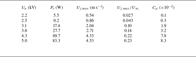
In total, six cases with increasing discharge voltage amplitudes of 2.2–5.0 kV are selected to characterise the performance of the plasma actuator. By integrating the voltage–current product over time (Fang et al. Reference Fang, Zong, Zhang, Wu, Su, Liang and Bian2024), the average power consumption ( $P_c$ ) of the plasma actuator in different cases is estimated, as listed in table 2.

Table 2.

Performance metrics of the plasma actuator at increasing discharge voltage.

Figure 6.

Profiles of the mean streamwise velocity pertaining to the baseline TBL at a streamwise location of $x/L = 0.5$ . The DNS data at a comparable momentum-thickness Reynolds number of $Re_\theta = 3630$ are plotted for validation (Schlatter & Örlü Reference Schlatter and Örlü2010).

Figure 7( $a$ ) shows a representative plasma jet velocity field obtained by PIV at $U_{a}$ = 5 kV. The maximum wall-normal jet velocity is determined to be $U_{j,max}$ = 4.5 m s⁻¹, with an uncertainty level of 0.046 m s⁻¹. This value is used to normalise the in-plane velocity magnitude ( $U_{j}$ ), resulting in a dimensionless quantity ranging from 0 to 1. Driven by the electrostatic body force, two opposing plasma jets originate at the junction of anodes and cathodes, accelerate towards the centre and bend upwards to form a wall-normal jet after collision. Since plasma jets are zero-net mass-flux jets, a clear downward replenishing flow can be observed between the wall-normal plasma jets, consistent with the observation in Zong et al. (Reference Zong, Wu, Su, Liang and Fang2023). As a result of this shear, a counter-rotating vortex pair induced by the entrainment of surrounding fluids can be identified in the two lateral sides of the wall-normal jet. The vortex cores of this counter-rotating vortex pair are highlighted in the streamwise vorticity field of figure 7( $b$ ). The thick black lines represent Q-criterion contours, with the contour level set as 6 % of the maximum Qvalue.

Figure 7.

( $a$ ) Time-averaged jet velocity and (b) vorticity fields induced by the plasma actuator array at $U_{a}=5$ kV. The pink and blue rectangles beneath the $x$ axis indicate the positions of anodes and cathodes, respectively. The green triangle highlights the position of peak jet velocity. Wall-normal profiles of the (c) blowing velocity, (d) suction velocity and (e) jet width. ( $f$ ) Variation of the jet momentum coefficient with increasing discharge voltage.

Figure 7( $c$ , $d$ ) shows the wall-normal variations of the blowing velocity ( $U_b$ ) above the anode centre at $z/L=0$ and the suction velocity ( $U_s$ ) above the cathode centre at $z/L=0.5$ . Regardless of the discharge voltage, $U_b$ exhibits a rapid initial increase followed by a slow decay when moving away from the wall. The peak value of $U_b$ occurs at approximately $y/L = 0.2$ , lower than that of the annular plasma jet ( $0.5L$ ) reported in Santhanakrishnan & Jacob (Reference Santhanakrishnan and Jacob2007). Compared with $U_b$ , an opposite variation trend is shown by $U_s$ , and the peak suction velocity seems to be only half of the maximum blowing velocity. Figure 7( $e$ ) further shows the wall-normal evolution of the jet width (denoted as $w_{\textit{jet}}$ ), extracted from the velocity contour. Note that the jet width here is defined as the spanwise extent of the blowing velocity, and the corresponding measurement uncertainty estimated from 200 instantaneous velocity fields is about 0.054 mm. Consequently, the jet width reaches a typical value of $w_0=0.4L$ at the position of maximum blowing velocity, increasing monotonically to $L$ afterwards. Based on the peak jet velocity ( $U_{j,max}$ ) and the typical jet width ( $w_0$ ), the momentum coefficient can be estimated from (3.1):

(3.1) \begin{equation} \displaystyle C_\mu =\frac {\rho U_{j,max}^2 w_0 L_p }{\rho U_\infty ^2\delta _{99}L}, \end{equation}

where $L_p$ is the streamwise length of the plasma actuator (100 mm). As shown in figure 7(f), $C_{\mu}$ increases rapidly with the discharge voltage, reaching 0.083 at $U_a = 5$ kV.

3.3. Drag reduction with open-loop periodical control

In open-loop control, the upstream hot-film sensors are disabled, and unsteady periodical waveforms are directly imposed on the plasma actuator. At a given discharge voltage amplitude, different combinations of modulation frequency and duty cycle are tested to get a two-dimensional drag-reduction map. In total, five modulation frequencies ( $f_m$ = 50, 100, 200, 500, 1000 Hz) and five duty cycles ( $D_c$ = 10 %, 20 %, 50 %, 70 %, 100 %) are selected. For each combination, the output signals of HW1 and HW2 are acquired for 10 s at a sampling frequency of 5 kHz. These signals are first converted to shear stresses using the calibration curves shown in figure 3. Then, the time-averaged shear stress values are used to calculate the drag-reduction magnitude for each sensor (denoted as $\textit{DR}^i$ ), as well as the mean relative drag reduction ( $\overline{\textit{DR}}$ ):

(3.2) \begin{equation} \left \lbrace \begin{array}{ll} \displaystyle \textit{DR}^i=\frac {\tau ^i_{bl}-\tau ^i_{at}}{\tau ^i_{bl}} \hspace{10pt} \textrm{for}\;\;i=[1,2] \\[15pt] \overline{\textit{DR}}=0.5(\textit{DR}^1+\textit{DR}^2), \end{array} \right . \end{equation}

where $\tau ^i_{bl}$ and $\tau ^i_{at}$ represent the wall shear stress measured by the $i$ th ( $i=1,2$ ) sensor under baseline and actuated conditions, respectively. In this process, measurement uncertainty can be introduced by the voltage acquisition and the fourth-order polynomial calibration. Following the error propagation rule, the total relative measurement uncertainty of $\overline{\textit{DR}}$ caused by these two factors is estimated to be 1.7 %.

Figure 8.

Drag-reduction map obtained by open-loop periodical control at ( $a$ ) $U_a$ = 4.3 kV and ( $b$ ) $U_a$ = 5 kV. The thin dashed black lines are contour lines plotted in a step of 1 %. The thick green lines denote contour lines of $\overline{\textit{DR}}$ = 0. The yellow circles indicate the positions of maximum drag reduction.

Figure 8 presents the drag variation maps spanned by modulation frequency and duty cycle, measured at representative discharge voltages of $U_a$ = 4.3 and 5 kV. For comparison, the jet momentum coefficient values are labelled as an extra axis. Using the free-stream velocity and boundary-layer thickness to normalise the modulation frequency, a dimensionless frequency in the form of $F_m^*=f_m\delta _{99}/U_\infty$ can be derived. Morphologically, the two drag-reduction maps are similar, with the drag-increase and drag-reduction zones approximately divided by $D_c = 50\,\%$ . In the upper half-map (drag-increase zone), the duty cycle seems to play a more influential role than the modulation frequency, since the drag-increase magnitude increases monotonically with $D_c$ yet varies marginally with $F_m^\ast$ . Drag-reduction zone is mainly found in the low-duty-cycle range of $10\,\%\leqslant D_c\leqslant 40\,\%$ , consistent with the results in Fang et al. (Reference Fang, Zong, Zhang, Wu, Su, Liang and Bian2024) where a unidirectional plasma jet array was adopted and positive drag reduction was only observed under weak actuation. At $U_a$ = 4.3 kV, the maximum drag reduction (2.3 %) is found in the lower-left corner of the map, corresponding to an electrical setting of $D_c$ = 20 % and $F_m^\ast$ = 0.22 ( $f_m$ = 200 Hz). After increasing the voltage to $U_a$ = 5 kV, although the actuation strength has been boosted noticeably, the peak drag-reduction magnitude (2.3 %) and the optimal electrical setting ( $D_c$ = 20 % and $F_m^\ast$ = 0.55) remain approximately the same. This implies that effective turbulent drag reduction requires a fine-tuned plasma force. This contrasts with flow separation control, where the control effectiveness almost always increases with the actuation strength (Karthikeyan & Harish Reference Karthikeyan and Harish2025).

4.1. A typical learning process

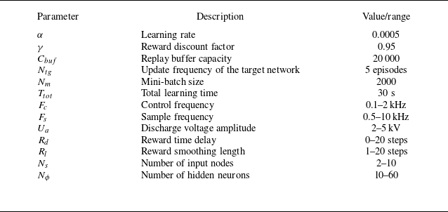
Extensive settings are involved in DRL control, as listed in table 3. The first five parameters are chosen empirically and fixed throughout this study, while the rest are tuned in appropriate ranges to achieve the best learning performance. These tunable hyper-parameters can be roughly divided into three categories: control-related parameters, network layout parameters and reward-shaping parameters. The control-related parameters include the amplitude of the discharge voltage ( $U_a$ ), the sample frequency of the sensor signals ( $F_s$ ) and the control loop frequency ( $F_c$ ). The network layout parameters mainly refer to the number of input nodes ( $N_s$ ) and the number of hidden neurons ( $N_\phi$ ). The reward-shaping parameters consist of the reward time delay ( $R_d$ ) and the reward smoothing length ( $R_l$ ) (see (2.4)). In the present study, the sample frequency is always chosen as five times the control frequency, to guarantee that in each control period, five fresh state vectors with 10 elements have been replenished into the S-FIFO. Correspondingly, the network input dimension ranges from 2 to 10.

Table 3.

Settings involved in the DQN control.

The above-mentioned tunable hyper-parameters constitute a six-element setting vector: $[U_a, F_c, R_d, R_l, N_s, N_\phi ]$ . To ensure reproducibility in repeat runs, the neural network is initialised with the same seed, providing a consistent starting point for training. For each case, the total learning time is set as $T_{tot}$ = 30 s. Detailed convergence check shows that after constant training of approximately 15 s, the Q-value functions begin to vary marginally, as well as the policy represented by the Q-network. Therefore, the present setting of total learning time is sufficient to ensure policy stabilisation in the final evaluation stage. Each learning process is split into three substages, according to the variation of $\varepsilon$ in the epsilon-greedy strategy (Zong et al. Reference Zong, Wu, Li, Su and Liang2025). Specifically, the first stage is called baseline test stage ( $t\leqslant 0.5\textrm{ s}$ ), where no plasma actuation is applied ( $a_t = 0$ ) and the exploration probability $\varepsilon$ is fixed to 0. In the subsequent training stage ( $0.5\textrm{ s}\lt t\lt 20 \textrm{ s}$ ), the exploration probability decays linearly from an initial value of 0.5–0, guiding the agent to explore the vast control space. For the final evaluation stage ( $20\textrm{ s}\leqslant t\leqslant 30 \textrm{ s}$ ), no more training is performed and the learnt policy is executed deterministically according to: $a_t = \textrm{argmax}\{\textbf{Q}({\boldsymbol{x}}_{\boldsymbol{t}}, a_t)\}$ .

As a first attempt of DRL control, the experience gained from open-loop periodical control is leveraged to guide the selection of hyper-parameters. Specifically, the voltage amplitude is chosen to be $U_a$ = 4.3 kV, and the control frequency is set as $F_c$ = 200 Hz, equal to the optimal modulation frequency found in figure 8( $a$ ). Other hyper-parameters are configured as: $[R_d, R_l, N_s, N_\phi ]$ = [0, 5, 2, 20]. Figure 9( $a$ – $d$ ) plots the time evolution of instant reward ( $r_t$ ), mean drag reduction ( $\overline{\textit{DR}}$ ), individual drag reduction ( $\textit{DR}^i$ ) and actuation probability ( $P_a$ ). Here, $P_a$ is defined as the switch-on probability of the plasma actuator in a short time period (0.5 s in this study), which has similar meaning to the duty cycle in open-loop control. Shaded regions in these plots represent error bands computed from three repeat measurements.

Figure 9.

Time evolution of ( $a$ ) the instant reward $r_t$ , ( $b$ ) the mean drag reduction $\overline{\textit{DR}}$ , ( $c$ ) the individual drag reduction $\textit{DR}^i$ and ( $d$ ) the actuation probability $P_a$ . ( $e$ ) The PDF of wall shear stresses measured by the downstream hot wires. The green dashed lines indicate the values pertaining to the optimal open-loop control.

As is evident, the variation trend of the instant reward agrees well with that of the mean drag reduction, both of which increase steadily at $t\leqslant$ 20 s. Individually, since HW1 and HW2 are located, respectively, in the wakes of the plasma-induced downwash and upwash zones (see figure 7 $a$ ), opposite drag variations are manifested. In the upwash zone, low-speed fluids in the viscous sublayer are transported to the buffer layer, which reduces drag. Conversely, in the downwash zone, high-speed fluids in the outer layer are swept towards the wall, leading to a drag increase (Fang et al. Reference Fang, Zong, Zhang, Wu, Su, Liang and Bian2024; Benard et al. Reference Benard, Bonnet and Moreau2024). The initial drag reduction earned by HW1 reaches as high as 10 % at $t\leqslant 5$ s. However, this gain is completely counteracted by the drag increase measured by HW2. Subsequently, the drag variation magnitudes caused by both HW1 and HW2 decrease monotonically, but at different rates. Eventually, the drag-reduction effect of HW1 wins out, and by averaging the value of $\overline{\textit{DR}}$ in the evaluation stage ( $20\textrm{ s}\leqslant t\leqslant 30\textrm{ s}$ ), the mean drag reduction achieved by DRL is determined to be 2.9 %, slightly higher than the optimal value in open-loop control (2.3 %) at the same voltage setting of 4.3 kV. Additionally, during the course of DRL, the actuation probability gradually decreases from an initial value of 30 % towards a final value of 20 %. This final value aligns well with the optimal duty cycle identified in figure 8( $a$ ). In figure 9( $e$ ), the probability density functions (PDFs) of the instantaneous wall shear stresses measured by HW1 and HW2 (denoted as $\tau ^1$ and $\tau ^2$ ) are further plotted. Note that for the actuated case, only the data in the evaluation stage are used. Compared with the baseline, the distribution of $\tau ^1$ shifts to the left after plasma actuation, and its kurtosis increases. On the contrary, the distribution of $\tau ^2$ moves to the right, becoming flatter.

Based on the above analyses, it is fair to conclude that DRL-based closed-loop control outperforms open-loop control in all aspects. For the authors, the most impressive feature is probably the high efficiency. Specifically, identifying the optimal setting in open-loop control requires testing dozens of parameter combinations, which consumes approximately one hour of wind tunnel running time in this study (§ 3.3). In contrast, the FeDRL controller achieves superior performance by testing for only 30 s.

4.2. Impacts of the hyper-parameters

In this section, the impacts of reward time delay and reward smoothing length on the DRL control performance are first examined by keeping other hyper-parameters identical to those in the previous section. In total, six levels of $R_d$ ([0, 1, 2, 4, 6, 8], in units of control periods) and five levels of $R_l$ ([1, 2, 4, 6, 8], in units of control periods) are selected to construct a two-dimensional matrix, and the mean relative drag reduction achieved by DRL is plotted in figure 10( $a$ ). It is evident that the reward time delay plays a more critical role than the reward smoothing length. As the reward smoothing length increases, a marginal variation of the control performance is observed. In contrast, with increasing reward time delay, the mean drag-reduction magnitude goes up monotonically, reaching a peak value of $\overline{\textit{DR}}$ = 4 % at $R_d=8$ . Since this reward delay value hits the upper limit of our parameter setting, there might be a possibility that further increasing the reward delay can lead to more drag-reduction benefit. In future, studies with a wider parameter range are needed to validate the above conjecture.

Figure 10.

( $a$ ) Relative drag reduction achieved by DRL at different combinations of reward time delay and reward smoothing length. The thin dashed black lines are contour lines in a step size of 0.5 %. The yellow circle indicates the position of peak drag reduction. Impacts of the (b) control frequency, (c) number of input nodes and (d) number of hidden neurons on the relative drag-reduction magnitude.

Taking the results shown in figure 10( $a$ ) as a reference, the threshold value of $R_d$ above which the drag-reduction magnitude starts to exceed that of its open-loop control partner is estimated to be 3. Since the control period is $T_c=1/F_c=\textrm{5 ms}$ , a reward time delay of $R_d=3$ would imply a physical time delay of 15 ms, consistent with the convection time delay (14 ms) required for a disturbance to propagate from the upstream state detection sensors to the downstream reward evaluation sensors. Actually, it has long been recognised that proper formulation of the reward is crucial to the performance of DRL in AFC (Guastoni et al. Reference Guastoni, Rabault, Schlatter, Azizpour and Vinuesa2023). For the present study, since the control object (i.e. the TBL) has a strong convective feature, the consequence of an action does need some time to fully come into force. Thus, an instantaneous reward feedback mechanism ( $R_d = 0$ ) may lead to a temporal mismatch between the currently imposed action and its corresponding flow response. A time-delay window is therefore necessary to account for the arrival and duration of plasma-induced flow disturbances. To some extent, these windows function as the self-attention mechanism widely adopted in large-language models. Similar practices can be found in Sonoda et al. (Reference Sonoda, Liu, Itoh and Hasegawa2023) and Chen et al. (Reference Chen, Zong, Song, Wu, Liang and Xiang2024b ), where the instantaneous rewards are replaced with sliding-averaged rewards, to improve the algorithm’s learning efficiency.

Figure 10( $b$ ) plots the impact of control frequency on the DRL performance. Both $R_d$ and $R_l$ are fixed to 4. Intuitively, control frequency determines how fast the agent interacts with the flow environment, and thus can be normalised by the characteristic frequency of the TBL, resulting in a dimensionless control frequency in the form of $F_c^\ast =f_c\delta _{99}/U_\infty$ . As the control frequency increases from 100 to 2000 Hz ( $F_c^\ast {:}\;0.06\rightarrow 2.2$ ), the relative drag reduction first goes up rapidly from 1.2 % to 5 % and then remains approximately unchanged. The kink point of the variation occurs at $f_c=$ 1000 Hz, which, by coincidence, corresponds to a nice dimensionless frequency value of close to 1. Physically, this trend can be explained by the fact that a higher interaction frequency with the control object provides more information about the dynamics of the flow, such as the emergence of sweep and burst events crucial in wall turbulence. If the control frequency is an order of magnitude lower than the characteristic flow frequency, the controller perceives only random flow snapshots. These snapshots exhibit minimal correlation between consecutive measurements, making it impossible for the agent to understand the flow dynamics.

In addition to the control-related parameters and reward-shaping parameters, the network layout can also impact the performance of DRL (Chen et al. Reference Chen, Zong, Song, Wu, Liang and Xiang2024b ). Theoretically, increasing $N_s$ and $N_\phi$ should be beneficial. A larger $N_s$ allows the controller to better capture the historical evolution of the flow, while a larger $N_\phi$ enhances the network’s capacity to model complex nonlinear relationships. However, practically, as shown in figure 10( $c$ , $d$ ), the network layout parameters need to be chosen wisely to obtain a reasonable DRL control performance. Particularly, in the range of $20\leqslant N_\phi \leqslant 60$ , a decreasing trend of $\overline{\textit{DR}}$ is exhibited with increasing number of hidden neurons, signifying that complex network architectures are not necessarily better, presumably due to over-fitting. As for $N_s$ , considering the chaotic nature of the TBL, too many state inputs may confuse the learning of the agent under current control frequency (1000 Hz), making it difficult to pick out the states that need actuation.

4.3. Meta-learning of the hyper-parameters with PSO

Although the impacts of hyper-parameters have been examined in the previous section, the test cases only represent a few lines sampled from the multidimensional parameter space. To unlock the potential of DRL in drag reduction, it is necessary to resort to meta-learning, i.e. learning how to perform effective reinforcement learning with another intelligent algorithm. For this purpose, PSO is employed to search the optimal DRL setting in a six-dimensional space ( $[U_a, F_c, R_d, R_l, N_s, N_\phi ]$ ), and the detailed flowchart is sketched in figure 11 (Kennedy & Eberhart Reference Kennedy and Eberhart1995). The optimisation begins with a random initialisation of particle positions in Python, where each particle represents a hyper-parameter set within the bounds specified by table 3. These parameter sets are then transmitted to the LabVIEW program via TCP/IP for performance evaluation. Three repeat DRL controls are conducted for each parameter set, and the average drag-reduction magnitude, namely the fitness value, is sent back to the host computer. These fitness values are used to determine the positions of global and local best particles, based on which the swarm’s positions and velocities are updated. Finally, the above process is iterated until a terminal condition is reached. In total, 10 iterations of 100 particles are tested, and the inertia weight is assumed to be a linearly decreasing function of the iteration number, enabling PSO to have balanced global exploration capability in the early stage and local convergence capability in the later stage. Both the cognitive coefficient $c_1$ and social coefficient $c_2$ are set to 2, following the typical configuration in Kennedy & Eberhart (Reference Kennedy and Eberhart1995).

Figure 11.

Flowchart of hyper-parameter optimisation with PSO.

Figure 12( $a$ ) plots the evolution of $\overline{\textit{DR}}$ in PSO, where particles are represented by violet circles. The local-best particle in each generation and the global-best particle obtained during the course of optimisation are denoted as $p_{l,b}$ and $p_{g,b}$ , respectively. With increasing generation number, the fitness values of the particle swarm increase steadily. Particularly, in the first generation, the local-best individual already delivers a DRL control performance close to the optimal setting in § 4.2. After the fourth generation, $\overline{\textit{DR}}$ of the local-best particle in each generation oscillates slightly between 5 % and 6 % as a consequence of the algorithm’s exploration. Meanwhile, the global-best fitness shows a marginal increase. The final drag-reduction magnitude achieved by the global-best particle reaches 6.7 %, nearly three times that of the best case in open-loop control (2.3 %, obtained at $f_m$ = 200 Hz and $D_c$ = 20 %). The corresponding hyper-parameter setting is $[U_a, F_c, R_d, R_l, N_s, N_\phi ]$ = [5 kV, 1750 Hz, 11, 8, 8, 20], with a mean actuation probability of 24.3 %. For open-loop control with equivalent modulation frequency of $f_m$ = 1750 and duty cycle of $D_c$ = 24.3 %, the drag-reduction magnitude is interpolated to be only 0.7 %.

Figure 12.

Evolution of different parameters in PSO: ( $a$ ) mean relative drag reduction, ( $b$ ) actuation probability, ( $c$ ) voltage amplitude, ( $d$ ) control frequency, ( $e$ ) reward time delay, ( $f$ ) reward smoothing length, ( $g$ ) number of input nodes and ( $h$ ) number of hidden neurons. The green dashed line in (a) indicates the maximum drag-reduction level achieved by the open-loop control.

To understand the behaviour of PSO, the optimisation histories of the actuation probability and the six hyper-parameters are plotted in figure 12( $b$ – $h$ ). After the second generation, the input voltage stabilises at approximately 5 kV. Concurrently, the actuation probability drops below 20 %, and the control frequency increases rapidly. This trend indicates that the optimal DRL control adopts a high-energy high-frequency low-actuation-probability strategy. As with the reward-shaping parameters, the local-best value of $R_d$ pivots around 10 control steps, and an obvious decreasing trend of $R_l$ from 12 to 5 control steps is observed during the course of optimisation. The final reward-shaping parameters lie in the middle-right of figure 10( $a$ ), consistent with the previous section. For the network layout, the optimal number of input nodes ( $N_s$ ) remains at eight during the optimisation, implying that incorporating historical states into the network input can indeed enhance the learning performance. By contrast, the number of hidden neurons decreases monotonically with the generation number, which is consistent with the results shown in figure 10( $d$ ).