1 Introduction
Wall-bounded disperse two-phase flows play an important role in many environmental and industrial applications. Some examples include liquid–solid slurry pipelines, sediment deposition in marine flows, foreign debris in gas turbine engines and fluidized bed reactors. Accurate predictions of such flows are necessary in order to gain a detailed understanding of the fundamental processes taking place, and ultimately improve the design of engineering devices. Meanwhile, non-trivial interactions between the carrier fluid and particulate phase lead to a wide range of two-phase flow regimes that may exist simultaneously within a single flow.
Many studies on wall-bounded particle-laden flows consider moderately dilute suspensions with weak interphase coupling (see e.g. Kulick, Fessler & Eaton Reference Kulick, Fessler and Eaton1994; Wang & Squires Reference Wang and Squires1996; Rouson & Eaton Reference Rouson and Eaton2001; Yamamoto et al.
Reference Yamamoto, Potthoff, Tanaka, Kajishima and Tsuji2001; Marchioli & Soldati Reference Marchioli and Soldati2002; Picciotto, Marchioli & Soldati Reference Picciotto, Marchioli and Soldati2005; Pitton et al.
Reference Pitton, Marchioli, Lavezzo, Soldati and Toschi2012; Zhao, Andersson & Gillissen Reference Zhao, Andersson and Gillissen2013). In this regime, the majority of the underlying carrier-phase turbulence manifests from classical mean-shear production (Zhao et al.
Reference Zhao, Andersson and Gillissen2013; Richter Reference Richter2015). Experiments (e.g. Fessler, Kulick & Eaton Reference Fessler, Kulick and Eaton1994) and fully resolved (model-free) calculations (e.g. García-Villalba, Kidanemariam & Uhlmann Reference García-Villalba, Kidanemariam and Uhlmann2012) have shown that wakes generated by small (
 $d_{p}/\unicode[STIX]{x1D702}\ll 1$
) and large (
 $d_{p}/\unicode[STIX]{x1D702}\gg 1$
) particles (with
 $d_{p}$
the particle diameter and
 $\unicode[STIX]{x1D702}$
the Kolmogorov length scale) could have a direct contribution to the turbulent kinetic energy (TKE) production and dissipation even at low particle seedings. Tanaka (Reference Tanaka2017) performed fully resolved simulations of particle-laden homogeneous shear turbulence and showed that finite particle inertia generates mean slip velocities between the phases in both the streamwise and shear directions, resulting in a slower increase in fluid-phase TKE. When gravity is directed in the sheared direction, the Reynolds shear stress becomes relatively large between counter-rotating trailing vortices downstream of particles, which was found to contribute to a transient rapid increase in TKE (Tanaka Reference Tanaka2017).
When the mean mass loading
 $\unicode[STIX]{x1D6F7}$
, defined by the ratio of the specific masses of the particle and fluid phases, is order one or larger, the relative motion between the phases leads to additional sources of instabilities as a result of interphase coupling (Glasser, Sundaresan & Kevrekidis Reference Glasser, Sundaresan and Kevrekidis1998). Gualtieri, Battista & Casciola (Reference Gualtieri, Battista and Casciola2017) found that sub-Kolmogorov particles with
 $O(1)$
mass loading modify the energy spectrum in homogeneous shear flows, leading to a scaling law
 $E(k)\propto k^{-4}$
, with
 $k$
the wavenumber, that emerges at small scales where particle forcing balances viscous dissipation. The particles were found to drain energy from the carrier flow at large scales and release it back at small scales. Dritselis (Reference Dritselis2016) evaluated budgets of the Reynolds stress in a vertical channel flow seeded with sub-Kolmogorov particles at intermediate loading (
 $\unicode[STIX]{x1D6F7}\leqslant 0.5$
). Each term in the Reynolds-stress budget was found to decrease in the presence of particles. The extent to which the budgets were reduced was found to depend on the particle response time, with greater effect when collisions were included. It was observed that large flow scales are generally dragged by small inertial particles, while large inertial particles are capable of interacting with a wider range of moderate flow scales.
At significantly large mass loadings, particles self-organize into dense clusters that greatly impact the overall flow structure (e.g. Agrawal et al.
Reference Agrawal, Loezos, Syamlal and Sundaresan2001; Capecelatro, Desjardins & Fox Reference Capecelatro, Desjardins and Fox2014a
). Vreman et al. (Reference Vreman, Geurts, Deen, Kuipers and Kuerten2009) performed simulations of a high-mass-loading turbulent channel flow and found that when
 $\unicode[STIX]{x1D6F7}\gg 1$
, particle collisions have a large influence on the mean and root-mean-square velocities of each phase. Particles were also observed to decrease the thickness of the boundary layer and increase the skin friction. A similar modification to the near-wall velocity profile was observed in dense suspensions of neutrally buoyant particles (Picano, Breugem & Brandt Reference Picano, Breugem and Brandt2015; Lashgari et al.
Reference Lashgari, Picano, Breugem and Brandt2016; Santarelli, Roussel & Fröhlich Reference Santarelli, Roussel and Fröhlich2016; Lashgari, Picano & Costa Reference Lashgari, Picano, Costa, Breugem and Brandt2017). Even at small density ratios, significant turbulence modulation was observed in those studies, with three distinct regimes revealed by the Reynolds-stress budget: laminar, turbulent and inertial shear thickening, depending on the relative contribution from viscous and particle stresses on the momentum transfer across the channel. Capecelatro, Desjardins & Fox (Reference Capecelatro, Desjardins and Fox2016a
) recently performed simulations of high-mass-loading (
 $\unicode[STIX]{x1D6F7}=10$
) channel flows, demonstrating that in this regime the primary source of turbulence generation is a term that is proportional to the product of mass loading, drift velocity and mean slip between the phases, termed drag production. It was also shown that the fluid-phase Reynolds-stress budget differs significantly from what is observed in dilute particle-laden channel flows.
Surprisingly, it remains to be seen how wall-bounded particle-laden flows transition from the dilute limit in which classical mean-shear production is primarily responsible for generating fluid-phase TKE, to the high-mass-loading regime dominated by drag production. In this study, we explore the transition between these two states and identify the key mechanisms responsible for the striking differences. Eulerian–Lagrangian simulations are conducted for
 $0\leqslant \unicode[STIX]{x1D6F7}\leqslant 20$
in a
 $Re_{\unicode[STIX]{x1D70F}}=300$
turbulent channel flow at two Stokes numbers. Details on the mathematical formulation are presented in § 2. The vertical channel configuration is then described in § 3, and visualizations and energy budgets are reported in § 4.
2 Mathematical description
In this section we present the governing equations describing solid spherical particles suspended in a constant-density gas-phase channel. Unlike in single-phase flows where the Navier–Stokes equations can be directly averaged to obtain a set of mean-flow equations (Pope Reference Pope2000), special care needs to be taken for turbulent multiphase flows. As discussed in Fox (Reference Fox2014), averaging the microscale equations (i.e. a model that resolves the boundary layers around each particle), will fail to retain important fluid–particle coupling terms. For example, in flows where fluctuations in the particle-phase volume fraction
 $\unicode[STIX]{x1D6FC}_{p}$
play an important role (see, e.g. Capecelatro, Desjardins & Fox Reference Capecelatro, Desjardins and Fox2015), the averaged microscale equations will not contain information about such fluctuations. Deriving the mean-flow equations starting from a mesoscopic description will retain more physics by explicitly accounting for important interphase coupling terms. The mesoscale equations are presented in the following section, followed by the macroscopic mean-flow equations.
2.1 Volume-filtered Euler–Lagrange equations
The displacement of an individual particle
 $i$
with diameter
 $d_{p}$
is calculated via
 $$\begin{eqnarray}\displaystyle & \displaystyle \boldsymbol{v}_{p}^{(i)}={\displaystyle \frac{\text{d}\boldsymbol{x}_{p}^{(i)}}{\text{d}t}}\quad \text{and}\quad {\displaystyle \frac{\text{d}\boldsymbol{v}_{p}^{(i)}}{\text{d}t}}=\boldsymbol{{\mathcal{A}}}^{(i)}+\boldsymbol{F}_{c}^{(i)}+\boldsymbol{g}, & \displaystyle\end{eqnarray}$$
where
 $\boldsymbol{v}_{p}^{(i)}(t)$
is the instantaneous particle velocity at time
 $t$
,
 $\boldsymbol{g}=[g,~0,~0]^{\mathsf{T}}$
is the acceleration due to gravity and
 $\boldsymbol{F}_{c}$
is the collision force modelled using a modified soft-sphere approach (Capecelatro & Desjardins Reference Capecelatro and Desjardins2013) originally proposed by Cundall & Strack (Reference Cundall and Strack1979). In this work, we consider inelastic collisions with a coefficient of restitution of
 $0.9$
for both particle–particle and particle–wall collisions. The interphase-exchange term is given by
 $$\begin{eqnarray}\displaystyle & \displaystyle \boldsymbol{{\mathcal{A}}}^{(i)}={\displaystyle \frac{1}{\unicode[STIX]{x1D70F}_{p}}}\left(\boldsymbol{u}_{f}[\boldsymbol{x}_{p}^{(i)}]-\boldsymbol{v}_{p}^{(i)}\right)-{\displaystyle \frac{1}{\unicode[STIX]{x1D70C}_{p}}}\unicode[STIX]{x1D735}p_{f}^{\star }[\boldsymbol{x}_{p}^{(i)}]+{\displaystyle \frac{1}{\unicode[STIX]{x1D70C}_{p}}}\unicode[STIX]{x1D735}\boldsymbol{\cdot }\unicode[STIX]{x1D748}_{f}[\boldsymbol{x}_{p}^{(i)}], & \displaystyle\end{eqnarray}$$
where
 $\unicode[STIX]{x1D70F}_{p}=\unicode[STIX]{x1D70C}_{p}d_{p}^{2}/(18\unicode[STIX]{x1D70C}_{f}\unicode[STIX]{x1D708}_{f})$
is the particle relaxation time, with
 $\unicode[STIX]{x1D70C}_{p}$
and
 $\unicode[STIX]{x1D70C}_{f}$
the particle- and fluid-phase material densities, respectively, and
 $\unicode[STIX]{x1D708}_{f}$
is the kinematic viscosity of the fluid. The fluid velocity
 $\boldsymbol{u}_{f}=[u_{f},~v_{f},~w_{f}]^{\mathsf{T}}$
, modified pressure gradient
 $\unicode[STIX]{x1D735}p_{f}^{\star }$
and divergence of the viscous-stress tensor
 $\unicode[STIX]{x1D735}\boldsymbol{\cdot }\unicode[STIX]{x1D748}_{f}$
are taken at
 $\boldsymbol{x}_{p}^{(i)}$
, the centre position of particle
 $i$
. The term
 $\unicode[STIX]{x1D735}p_{f}^{\star }$
is a body force that contains the hydrodynamic pressure
 $p_{f}$
and is adjusted dynamically in order to maintain a constant mass flow rate in the channel.
To account for the presence of particles in the fluid phase without requiring to resolve the boundary layers around individual particles, a volume filter is applied to the constant-density Navier–Stokes equations (Anderson & Jackson Reference Anderson and Jackson1967), thereby replacing the point variables (fluid velocity, pressure, etc.) by smoother, locally filtered fields. The volume-filtered conservation equations for a constant-density fluid are given by
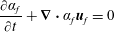 $$\begin{eqnarray}\displaystyle & \displaystyle {\displaystyle \frac{\unicode[STIX]{x2202}\unicode[STIX]{x1D6FC}_{f}}{\unicode[STIX]{x2202}t}}+\unicode[STIX]{x1D735}\boldsymbol{\cdot }\unicode[STIX]{x1D6FC}_{f}\boldsymbol{u}_{f}=0 & \displaystyle\end{eqnarray}$$
and
 $$\begin{eqnarray}\displaystyle & \displaystyle {\displaystyle \frac{\unicode[STIX]{x2202}\unicode[STIX]{x1D6FC}_{f}\boldsymbol{u}_{f}}{\unicode[STIX]{x2202}t}}+\unicode[STIX]{x1D735}\boldsymbol{\cdot }(\unicode[STIX]{x1D6FC}_{f}\boldsymbol{u}_{f}\otimes \boldsymbol{u}_{f})=-{\displaystyle \frac{1}{\unicode[STIX]{x1D70C}_{f}}}\unicode[STIX]{x1D735}p_{f}^{\star }+\unicode[STIX]{x1D735}\boldsymbol{\cdot }\unicode[STIX]{x1D748}_{f}-{\displaystyle \frac{\unicode[STIX]{x1D70C}_{p}}{\unicode[STIX]{x1D70C}_{f}}}\unicode[STIX]{x1D6FC}_{p}\boldsymbol{{\mathcal{A}}}+\unicode[STIX]{x1D6FC}_{f}\boldsymbol{g}, & \displaystyle\end{eqnarray}$$
where
 $\unicode[STIX]{x1D6FC}_{f}$
is the fluid-phase volume fraction and
 $\unicode[STIX]{x1D6FC}_{p}=1-\unicode[STIX]{x1D6FC}_{f}$
. The fluid-phase viscous-stress tensor is defined as
 $$\begin{eqnarray}\displaystyle & \displaystyle \unicode[STIX]{x1D748}_{f}=\left(\unicode[STIX]{x1D708}_{f}+\unicode[STIX]{x1D708}_{f}^{\star }\right)\left[\unicode[STIX]{x1D735}\boldsymbol{u}_{f}+\left(\unicode[STIX]{x1D735}\boldsymbol{u}_{f}\right)^{\mathsf{T}}-{\textstyle \frac{2}{3}}\unicode[STIX]{x1D735}\boldsymbol{\cdot }\boldsymbol{u}_{f}\unicode[STIX]{x1D644}\right], & \displaystyle\end{eqnarray}$$
where
 $\unicode[STIX]{x1D644}$
is the identity tensor and
 $\unicode[STIX]{x1D708}^{\star }$
is an effective viscosity that accounts for enhanced dissipation due to unresolved fluid velocity fluctuations generated at the particle scale (Gibilaro et al.
Reference Gibilaro, Gallucci, Di Felice and Pagliai2007). Details on the interphase-exchange term
 $\boldsymbol{{\mathcal{A}}}$
are discussed in § 3.2.
2.2 Phase-averaged flow equations
Analogous to Favre averaging in variable density flows, the phase average (PA) denoted by
 $\langle (\cdot )\rangle _{f}=\langle \unicode[STIX]{x1D6FC}_{f}(\cdot )\rangle /\langle \unicode[STIX]{x1D6FC}_{f}\rangle$
is useful in multiphase modelling. Here, angled brackets denote an average in the homogeneous
 $x$
- and
 $z$
-directions, i.e.
 $\langle (\cdot )\rangle (y)=\int \int (\cdot )\,\text{d}x\,\text{d}z$
, with
 $y$
the wall-normal direction. Fluctuations about the PA fluid velocity are expressed as
 $\boldsymbol{u}_{f}^{\prime \prime \prime }(\boldsymbol{x},t)=\boldsymbol{u}_{f}(\boldsymbol{x},t)-\langle \boldsymbol{u}_{f}\rangle _{f}$
, with
 $\langle \boldsymbol{u}_{f}^{\prime \prime \prime }\rangle _{f}=0$
. It is important to note that because the fluid velocity is correlated to volume fraction fluctuations,
 $\langle \boldsymbol{u}_{f}^{\prime \prime \prime }\rangle \neq 0$
in general. With this, the PA fluid TKE is
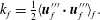 $$\begin{eqnarray}\displaystyle & \displaystyle k_{f}={\textstyle \frac{1}{2}}\langle \boldsymbol{u}_{f}^{\prime \prime \prime }\boldsymbol{\cdot }\boldsymbol{u}_{f}^{\prime \prime \prime }\rangle _{f}. & \displaystyle\end{eqnarray}$$
Similarly, the PA operator with respect to the particle phase can be defined via
 $\langle (\cdot )\rangle _{p}=\langle \unicode[STIX]{x1D6FC}_{p}(\cdot )\rangle /\langle \unicode[STIX]{x1D6FC}_{p}\rangle$
, with fluctuations about the PA particle velocity given by
 $\boldsymbol{u}_{p}^{\prime \prime }(\boldsymbol{x},t)=\boldsymbol{u}_{p}(\boldsymbol{x},t)-\langle \boldsymbol{u}_{p}\rangle _{p}$
. Here,
 $\boldsymbol{u}_{p}=[u_{p},~v_{p},~w_{p}]^{\mathsf{T}}$
is the spatially correlated component of the particle velocity (Février, Simonin & Squires Reference Février, Simonin and Squires2005; Capecelatro, Pepiot & Desjardins Reference Capecelatro, Pepiot and Desjardins2014b
) used in constructing the particle-phase TKE, given by
 $$\begin{eqnarray}\displaystyle & \displaystyle k_{p}={\textstyle \frac{1}{2}}\langle \boldsymbol{u}_{p}^{\prime \prime }\boldsymbol{\cdot }\boldsymbol{u}_{p}^{\prime \prime }\rangle _{p}. & \displaystyle\end{eqnarray}$$
As described in Capecelatro et al. (Reference Capecelatro, Desjardins and Fox2015), special care needs to be taken when decomposing the local particle velocity
 $\boldsymbol{v}_{p}^{(i)}$
into its spatially correlated and uncorrelated components, i.e.
 $\boldsymbol{v}_{p}^{(i)}=\boldsymbol{u}_{p}[\boldsymbol{x}_{p}^{(i)}]+\unicode[STIX]{x1D739}v_{p}^{(i)}$
, where
 $\unicode[STIX]{x1D739}v_{p}^{(i)}$
represents the random uncorrelated motion used in defining the granular temperature (Février et al.
Reference Février, Simonin and Squires2005)
 $$\begin{eqnarray}\displaystyle & \displaystyle \unicode[STIX]{x1D6E9}={\textstyle \frac{1}{3}}\unicode[STIX]{x1D739}v_{p}^{(i)}\boldsymbol{\cdot }\unicode[STIX]{x1D739}v_{p}^{(i)}. & \displaystyle\end{eqnarray}$$
With these definitions, the total granular energy is
 $$\begin{eqnarray}\displaystyle & \displaystyle \unicode[STIX]{x1D705}=k_{p}+{\textstyle \frac{3}{2}}\langle \unicode[STIX]{x1D6E9}\rangle _{p}. & \displaystyle\end{eqnarray}$$
In fully developed two-phase vertical channel flows, the evolution of
 $k_{f}$
is given by (Capecelatro et al.
Reference Capecelatro, Desjardins and Fox2016a
)
 $$\begin{eqnarray}\displaystyle {\displaystyle \frac{1}{\langle \unicode[STIX]{x1D6FC}_{f}\rangle }}\frac{\text{d}}{\text{d}y}\left({\displaystyle \frac{1}{2}}\langle \unicode[STIX]{x1D6FC}_{f}\rangle \langle v_{f}^{\prime \prime \prime }\boldsymbol{u}_{f}^{\prime \prime \prime }\boldsymbol{\cdot }\boldsymbol{u}_{f}^{\prime \prime \prime }\rangle _{f}+{\mathcal{E}}\right)={\mathcal{P}}_{shear}-\unicode[STIX]{x1D700}+{\mathcal{D}}{\mathcal{E}}+{\mathcal{D}}{\mathcal{P}}. & & \displaystyle\end{eqnarray}$$
The terms on the left-hand side and first two terms on the right-hand side of (2.10) do not involve mixed statistics (i.e. fluid–particle correlations) and have the same form as in single-phase turbulent flow (Pope Reference Pope2000). The triple correlation
 $(1/2)\langle v_{f}^{\prime \prime \prime }\boldsymbol{u}_{f}^{\prime \prime \prime }\boldsymbol{\cdot }\boldsymbol{u}_{f}^{\prime \prime \prime }\rangle _{f}$
will be referred to hereinafter as turbulent convection. The term containing pressure redistribution and viscous diffusion,
 $$\begin{eqnarray}\displaystyle & \displaystyle {\mathcal{E}}=\langle pv_{f}^{\prime \prime \prime }\rangle /\unicode[STIX]{x1D70C}_{f}-\langle \unicode[STIX]{x1D748}_{f,y}\boldsymbol{\cdot }\boldsymbol{u}_{f}^{\prime \prime \prime }\rangle , & \displaystyle\end{eqnarray}$$
typically becomes important in near-wall regions of the flow. The dissipation rate is given by
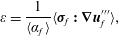 $$\begin{eqnarray}\displaystyle & \displaystyle \unicode[STIX]{x1D700}=\frac{1}{\langle \unicode[STIX]{x1D6FC}_{f}\rangle }\langle \unicode[STIX]{x1D748}_{f}\boldsymbol{ : }\unicode[STIX]{x1D735}\boldsymbol{u}_{f}^{\prime \prime \prime }\rangle , & \displaystyle\end{eqnarray}$$
and in the absence of a disperse phase, production due to mean shear, given by
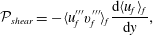 $$\begin{eqnarray}\displaystyle & \displaystyle {\mathcal{P}}_{shear}=-\langle u_{f}^{\prime \prime \prime }v_{f}^{\prime \prime \prime }\rangle _{f}{\displaystyle \frac{\text{d}\langle u_{f}\rangle _{f}}{\text{d}y}}, & \displaystyle\end{eqnarray}$$
is the primary mechanism by which
 $k_{f}$
is generated.
The remaining terms in the Reynolds-stress balance contain fluid–particle correlations that become important when interphase coupling is significant. The drag-dissipation-and-exchange rate
 $$\begin{eqnarray}\displaystyle & \displaystyle {\mathcal{D}}{\mathcal{E}}={\displaystyle \frac{\unicode[STIX]{x1D719}}{\unicode[STIX]{x1D70F}_{p}}}(\langle \boldsymbol{u}_{f}^{\prime \prime \prime }\boldsymbol{\cdot }\boldsymbol{u}_{p}^{\prime \prime }\rangle _{p}-\langle \boldsymbol{u}_{f}^{\prime \prime \prime }\boldsymbol{\cdot }\boldsymbol{u}_{f}^{\prime \prime \prime }\rangle _{p}) & \displaystyle\end{eqnarray}$$
describes how the turbulent kinetic energies are both dissipated and exchanged between the phases, where
 $\unicode[STIX]{x1D719}(y)=\unicode[STIX]{x1D70C}_{p}\langle \unicode[STIX]{x1D6FC}_{p}\rangle /(\unicode[STIX]{x1D70C}_{f}\langle \unicode[STIX]{x1D6FC}_{f}\rangle )$
is the average mass loading. Finally, the drag-production term
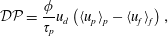 $$\begin{eqnarray}\displaystyle & \displaystyle {\mathcal{D}}{\mathcal{P}}={\displaystyle \frac{\unicode[STIX]{x1D719}}{\unicode[STIX]{x1D70F}_{p}}}u_{d}\left(\langle u_{p}\rangle _{p}-\langle u_{f}\rangle _{f}\right), & \displaystyle\end{eqnarray}$$
describes how fluid-phase turbulent kinetic energy is produced by a mean-velocity difference between the phases. The drift velocity, defined as
 $\boldsymbol{u}_{d}=\langle \boldsymbol{u}_{f}\rangle _{p}-\langle \boldsymbol{u}_{f}\rangle _{f}=\langle \boldsymbol{u}_{f}^{\prime \prime \prime }\rangle _{p}$
is directly responsible for generating fluid-phase TKE. In the limit
 $\unicode[STIX]{x1D719}\gg 1$
, drag production can be much larger than mean-gradient production (i.e.
 ${\mathcal{D}}{\mathcal{P}}\gg {\mathcal{P}}_{shear}$
), except very near the walls where
 $\boldsymbol{u}_{d}=\mathbf{0}$
due to the no-slip boundary condition for the fluid (Capecelatro et al.
Reference Capecelatro, Desjardins and Fox2016a
). It should be noted that (2.14) and (2.15) were formulated assuming Stokes drag. Accounting for drag coefficients with nonlinear dependencies on Reynolds number and volume fraction (e.g. Tenneti et al.
Reference Tenneti, Garg, Hrenya, Fox and Subramaniam2010) will result in higher-order terms that need to be accounted for (similarly to what appears in filtered two-fluid models, e.g. Igci et al.
Reference Igci, Andrews, Sundaresan, Pannala and O’Brien2008), but are neglected in this work. A discussion on the effect of using a nonlinear drag correlation can be found in appendix A.
3 Vertical particle-laden channel flow
3.1 System description
In this study we consider a turbulent channel flow with friction Reynolds number
 $Re_{\unicode[STIX]{x1D70F}}=300$
based on the channel half-width
 $\unicode[STIX]{x1D6FF}$
and
 $u_{\unicode[STIX]{x1D70F}}$
, the friction velocity of the corresponding unladen channel. The domain size is
 $20\unicode[STIX]{x1D6FF}\times 2\unicode[STIX]{x1D6FF}\times 3\unicode[STIX]{x1D6FF}$
in the streamwise (
 $x$
), wall-normal (
 $y$
) and spanwise (
 $z$
) directions, respectively. Periodic boundary conditions are imposed in the homogeneous
 $x$
- and
 $z$
-directions with gravity
 $g=-9.81~\text{m}~\text{s}^{-2}$
acting in
 $x$
. Uniform mesh spacing is imposed in the
 $x$
- and
 $z$
-directions of size
 $\unicode[STIX]{x0394}x^{+}=\unicode[STIX]{x0394}z^{+}=4.6$
, with a total grid size of
 $1250\times 138\times 188$
. Here, the superscript
 $+$
denotes normalization with the viscous scales for length
 $\unicode[STIX]{x1D708}/u_{\unicode[STIX]{x1D70F}}$
and time
 $\unicode[STIX]{x1D708}/u_{\unicode[STIX]{x1D70F}}^{2}$
. The mesh spacing is continuously stretched in the wall-normal direction as described in Kim, Moin & Moser (Reference Kim, Moin and Moser1987), with
 $y_{j}=\cos \unicode[STIX]{x1D703}_{j}$
, for
 $\unicode[STIX]{x1D703}_{j}=(j-1)\unicode[STIX]{x03C0}/(N_{y}-1)$
,
 $j=1,2,\ldots ,N_{y}$
, where
 $N_{y}$
is the number of grid points in
 $y$
. This corresponds to a maximum wall-normal spacing of
 $\unicode[STIX]{x0394}y^{+}=6.78$
at the channel centre, and
 $\unicode[STIX]{x0394}y^{+}=0.08$
at the channel wall.
Once the flow reaches a statistically stationary state, the channel is seeded with a random distribution of solid spherical particles. The number of particles used in each simulation is determined based on the mean mass loading, given by
 $$\begin{eqnarray}\displaystyle & \displaystyle \unicode[STIX]{x1D6F7}={\displaystyle \frac{\unicode[STIX]{x1D70C}_{p}}{\unicode[STIX]{x1D70C}_{f}}}{\displaystyle \frac{\overline{\unicode[STIX]{x1D6FC}}_{p}}{1-\overline{\unicode[STIX]{x1D6FC}}_{p}}}, & \displaystyle\end{eqnarray}$$
where the bar represents a volume-averaged quantity, and thus
 $\overline{\unicode[STIX]{x1D6FC}}_{p}=N_{p}V_{p}/V$
is the mean particle concentration within the channel with
 $N_{p}$
the total number of particles,
 $V_{p}=1/6\unicode[STIX]{x03C0}d_{p}^{3}$
is the particle volume and
 $V$
is the channel volume. The mass loading ranges from
 $0\leqslant \unicode[STIX]{x1D6F7}\leqslant 20$
corresponding to
 $0\leqslant \overline{\unicode[STIX]{x1D6FC}}_{p}\leqslant 0.01$
. For each case,
 $Re_{\unicode[STIX]{x1D70F}}$
remains the same and the density ratio is
 $\unicode[STIX]{x1D70C}_{p}/\unicode[STIX]{x1D70C}_{f}=2000$
. The influence of particle inertia is assessed by considering two sizes of particles with normalized particle diameters
 $d_{p}^{+}=0.74$
and
 $d_{p}^{+}=2.39$
, corresponding to
 $45.5$
and
 $144~\unicode[STIX]{x03BC}\text{m}$
glass beads in air, respectively, with bulk velocity
 $U_{b}=5~\text{m}~\text{s}^{-1}$
. The Stokes numbers based on
 $U_{b}$
and
 $\unicode[STIX]{x1D6FF}$
are
 $St_{\unicode[STIX]{x1D6FF}}=\unicode[STIX]{x1D70F}_{p}U_{b}/(2\unicode[STIX]{x1D6FF})=1.79$
and
 $17.86$
, and the Stokes numbers based on the friction velocity,
 $St_{\unicode[STIX]{x1D70F}}=\unicode[STIX]{x1D70F}_{p}u_{\unicode[STIX]{x1D70F}}/\unicode[STIX]{x1D6FF}=0.21$
and
 $2.1$
, for the small and large particles, respectively. The particle Reynolds number for these two classes of particles are
 $Re_{p}=d_{p}\unicode[STIX]{x1D70F}_{p}g/\unicode[STIX]{x1D708}=0.32$
and
 $10.0$
. The final relevant quantity is the characteristic cluster length scale, which can be estimated a priori as
 ${\mathcal{L}}=\unicode[STIX]{x1D70F}_{p}^{2}g$
(Agrawal et al.
Reference Agrawal, Loezos, Syamlal and Sundaresan2001; Igci et al.
Reference Igci, Andrews, Sundaresan, Pannala and O’Brien2008; Ozel, Fede & Simonin Reference Ozel, Fede and Simonin2013; Capecelatro et al.
Reference Capecelatro, Pepiot and Desjardins2014b
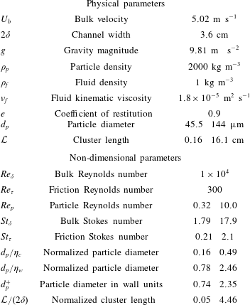
). The values used in the simulations are summarized in table 1. It is noteworthy that the normalized cluster length for the smaller Stokes number case is much less than unity, allowing for fully developed clusters; while for the larger Stokes number case cluster formation will be hindered by the channel walls. As the spatially correlated energy
 $k_{p}$
is largely associated with clusters at high mass loading (Capecelatro et al.
Reference Capecelatro, Desjardins and Fox2015), it can be expected that the larger Stokes number case will have higher levels of uncorrelated granular motion as compared to fully developed cluster-induced turbulence.
Fluid–particle parameters used in the channel simulations. Reynolds numbers are defined as
 $Re_{\unicode[STIX]{x1D6FF}}=2U_{b}\unicode[STIX]{x1D6FF}/\unicode[STIX]{x1D708}$
,
 $Re_{\unicode[STIX]{x1D70F}}=u_{\unicode[STIX]{x1D70F}}\unicode[STIX]{x1D6FF}/\unicode[STIX]{x1D708}$
and
 $Re_{p}=\unicode[STIX]{x1D70F}_{p}gd_{p}/\unicode[STIX]{x1D708}$
. The Stokes numbers are defined as
 $St_{\unicode[STIX]{x1D6FF}}=\unicode[STIX]{x1D70F}_{p}U_{b}/(2\unicode[STIX]{x1D6FF})$
and
 $St_{\unicode[STIX]{x1D70F}}=\unicode[STIX]{x1D70F}_{p}u_{\unicode[STIX]{x1D70F}}/\unicode[STIX]{x1D6FF}$
.
 $\unicode[STIX]{x1D702}_{c}$
and
 $\unicode[STIX]{x1D702}_{w}$
are the Kolmogorov length scales at the centre and wall of the single-phase channel flow, respectively.
3.2 Discretization
The Eulerian–Lagrangian equations are solved in NGA (Desjardins et al.
Reference Desjardins, Blanquart, Balarac and Pitsch2008), a fully conservative low Mach number solver with second-order accuracy in space and time. To transfer the fluid variables to the particle location, second-order tri-linear interpolation is used. To send the particle data back to the Eulerian mesh, a quantity
 $A^{(i)}(t)$
located at particle
 $i$
at time
 $t$
is projected to the grid via
 $$\begin{eqnarray}\displaystyle & \displaystyle \unicode[STIX]{x1D6FC}_{p}A(\boldsymbol{x},t)=\mathop{\sum }_{i=1}^{N_{p}}A^{(i)}(t){\mathcal{G}}(|\boldsymbol{x}-\boldsymbol{x}_{p}^{(i)}|)V_{p}, & \displaystyle\end{eqnarray}$$
where
 ${\mathcal{G}}$
is a filtering kernel with characteristic size
 $\unicode[STIX]{x1D6FF}_{f}=8d_{p}$
. This expression replaces the discontinuous Lagrangian data with an Eulerian field that is a smooth function of the spatial coordinate
 $\boldsymbol{x}$
. Using (3.2) with
 $A^{(i)}=1$
yields the particle volume fraction
 $\unicode[STIX]{x1D6FC}_{p}$
, and
 $A^{(i)}=\boldsymbol{{\mathcal{A}}}^{(i)}$
gives the momentum exchange term
 $\boldsymbol{{\mathcal{A}}}$
seen by the fluid in (2.4). In addition, setting
 $A^{(i)}=\boldsymbol{v}_{p}^{(i)}$
in (3.2) will yield
 $\boldsymbol{u}_{p}$
that appears in the drag-exchange and drag-production terms (2.14)–(2.15). It was found in our previous work that using a constant value of
 $\unicode[STIX]{x1D6FF}_{f}$
will provide a poor representation of the spatially correlated particle velocity in clustered gas–solid flows (Capecelatro et al.
Reference Capecelatro, Desjardins and Fox2015). Instead,
 $\unicode[STIX]{x1D6FF}_{f}$
is adjusted dynamically based on
 $\unicode[STIX]{x1D6FC}_{p}$
when computing
 $\boldsymbol{u}_{p}$
such that a constant number of particles,
 ${\mathcal{N}}_{p}$
, are sampled, i.e.
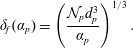 $$\begin{eqnarray}\displaystyle & \displaystyle \unicode[STIX]{x1D6FF}_{f}(\unicode[STIX]{x1D6FC}_{p})=\left(\frac{{\mathcal{N}}_{p}d_{p}^{3}}{\unicode[STIX]{x1D6FC}_{p}}\right)^{1/3}. & \displaystyle\end{eqnarray}$$
Applying the adaptive filter in an a priori manner to the particle data was found to yield a partition of
 $\unicode[STIX]{x1D705}$
into
 $k_{p}$
and
 $\langle \unicode[STIX]{x1D6E9}\rangle _{p}$
insensitive to the choice of parameters. Further details can be found in Capecelatro et al. (Reference Capecelatro, Desjardins and Fox2015, Reference Capecelatro, Desjardins and Fox2016a
).
Special care must be taken in the near-wall region where particles are larger than the mesh spacing due to the grid stretching employed. Because the projection used to transfer particle data to the mesh is tied to a filter size
 $\unicode[STIX]{x1D6FF}_{f}$
, and not the grid spacing (as is typically done when considering traditional interpolation), the grid-size-to-particle-diameter ratio is decoupled during the interphase-exchange process. To ensure the solution remains unconditionally stable, and the cost remains low when the grid spacing is significantly smaller than the filter size, equation (3.2) is solved using a two-step implicit filtering procedure (Capecelatro & Desjardins Reference Capecelatro and Desjardins2013). However, special care needs to be taken to properly account for inter-particle collisions in regions where the particle diameter is larger than the mesh spacing. To this end, a uniform auxiliary grid with spacing
 $2d_{p}$
is used to handle efficient collision detection throughout the domain. The numerical approach has been extensively validated for vertical wall-bounded flows in our previous work (Capecelatro et al.
Reference Capecelatro, Pepiot and Desjardins2014b
; Capecelatro & Desjardins Reference Capecelatro and Desjardins2015).
4 Results and discussion
4.1 Visualization
Visualizations of the instantaneous fluid-phase velocity and particle positions for
 $St_{\unicode[STIX]{x1D70F}}=2.1$
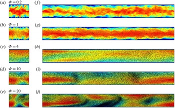
are shown in figure 1. The velocity field can be seen to change dramatically with increasing particle loading. At
 $\unicode[STIX]{x1D6F7}=0.2$
the flow closely resembles a single-phase channel with particles accumulating near the channel centreline. The turbulence intensity decreases at
 $\unicode[STIX]{x1D6F7}=1$
and particles appear to be more homogeneously distributed. At
 $\unicode[STIX]{x1D6F7}=4$
the velocity magnitude is significantly decreased and the channel is observed to have relaminarized (i.e. the spatial variations in fluid velocity are significantly reduced). Above
 $\unicode[STIX]{x1D6F7}=4$
, the velocity magnitude increases due to strong interphase coupling as particles spontaneously cluster. Jet bypassing can be observed at
 $\unicode[STIX]{x1D6F7}=20$
as clusters entrain the gas near the channel wall, causing high-speed jets to manifest in regions of low
 $\unicode[STIX]{x1D6FC}_{p}$
. It is important to note that with increasing mass loading the corresponding pressure drop increases in order to maintain equal mass flow rates for each case. Thus, relaminarization does not imply drag reduction, rather a switch from drag at the channel walls to drag at the particle surfaces. The specific dissipation mechanisms responsible for the observed behaviour will be quantified in later sections.
Instantaneous fields of fluid velocity magnitude in the
 $z$
–
 $y$
plane (a–e) and
 $x$
–
 $y$
plane (f–j) for
 $St_{\unicode[STIX]{x1D70F}}=2.1$
. Colour ranges from
 $|\boldsymbol{u}_{f}|/U_{b}=0.5$
(blue) to
 $|\boldsymbol{u}_{f}|/U_{b}=1.4$
(red). Black dots represent particle positions.
(a) Total energy based on the mixture density
 $\unicode[STIX]{x1D70C}_{f}\unicode[STIX]{x1D6FC}_{f}+\unicode[STIX]{x1D70C}_{p}\unicode[STIX]{x1D6FC}_{p}$
normalized by the corresponding energy of the single-phase flow and (b) skin-friction coefficient as a function of mass loading.
 $St_{\unicode[STIX]{x1D70F}}=0.21$
(○),
 $St_{\unicode[STIX]{x1D70F}}=2.1$
(♢) and corresponding single-phase values (– –).
4.2 Mean two-phase statistics
For each case presented in this work, the initial transient persists for approximately
 $10\unicode[STIX]{x1D70F}_{p}$
before reaching a fully developed statistically stationary state. After this initial transient, results are measured at each computational time step (
 $\unicode[STIX]{x0394}t=2\times 10^{-5}\unicode[STIX]{x1D70F}_{p}$
), over a duration of approximately
 $10\unicode[STIX]{x1D70F}_{p}$
. The total TKE, defined as
 $(\unicode[STIX]{x1D70C}_{f}\overline{\unicode[STIX]{x1D6FC}_{f}k_{f}}+\unicode[STIX]{x1D70C}_{p}\overline{\unicode[STIX]{x1D6FC}_{p}\unicode[STIX]{x1D705}})/\unicode[STIX]{x1D70C}_{m}$
based on the mixture density
 $\unicode[STIX]{x1D70C}_{m}=\unicode[STIX]{x1D70C}_{f}\overline{\unicode[STIX]{x1D6FC}}_{f}+\unicode[STIX]{x1D70C}_{p}\overline{\unicode[STIX]{x1D6FC}}_{p}$
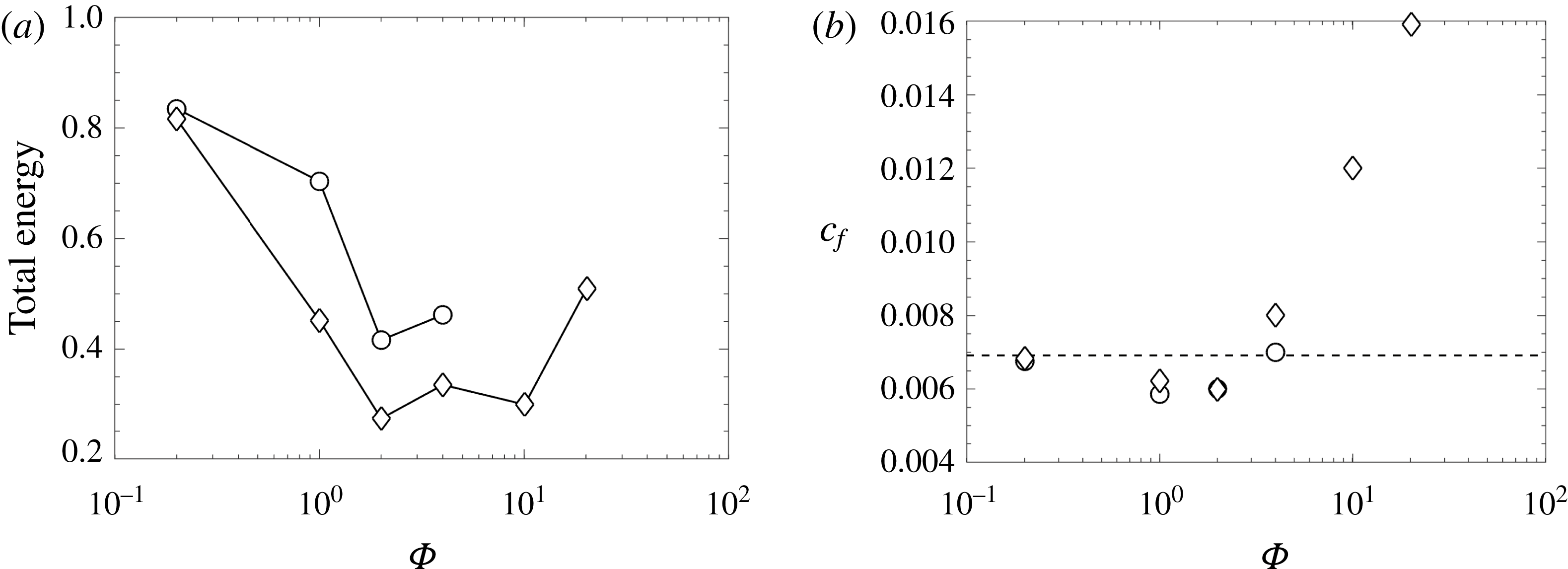
is shown in figure 2(a). The total TKE is observed to have non-monotonic behaviour. Because particles more closely follow fluid streamlines in the lower Stokes number flow, they exhibit higher correlated energy
 $k_{p}$
compared to the flows seeded with larger particles, giving rise to larger overall TKE. In the low-mass-loading regime, the level of fluid-phase TKE is reduced as particles are added to the flow (as shown by the energy budgets in later sections), and the additional energy by the particles are not sufficient to balance this loss. With
 $\unicode[STIX]{x1D6F7}>2$
interphase coupling gives rise to drag production, resulting in an overall increase in TKE.
The skin-friction coefficients of the channel flows based on the total force
 $F_{w}$
exerted by the flow on the channel walls and the bulk velocity are given by
 $$\begin{eqnarray}\displaystyle & \displaystyle c_{f}={\displaystyle \frac{F_{w}}{\unicode[STIX]{x1D70C}_{f}\unicode[STIX]{x1D6FC}_{f}SU_{b}^{2}}}, & \displaystyle\end{eqnarray}$$
where
 $S$
is the total wall surface area. As shown in figure 2(b), at low mass loading (
 $\unicode[STIX]{x1D6F7}\leqslant 2$
) the skin-friction coefficients are less than the unladen flow. Vreman (Reference Vreman2007) showed similar behaviour in turbulent particle-laden pipe flow. However, above
 $\unicode[STIX]{x1D6F7}=2$
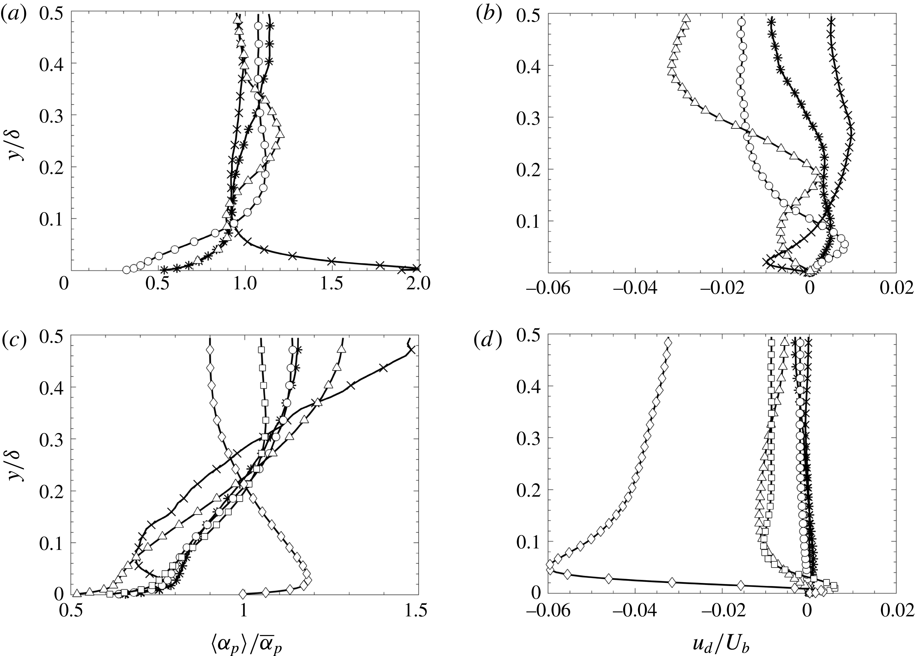
the skin-friction coefficients drastically increase with increasing loading due to enhancement in particle concentration near the wall, as seen in figure 3.
A transition in the particle distribution can be seen from the profiles of normalized volume fraction in figure 3(a,c). At low Stokes number and low mass loading, the channel flow exhibits similar phenomenon of turbophoresis reported in the literature (e.g. Marchioli & Soldati Reference Marchioli and Soldati2002), resulting in particle accumulating near the channel wall. At higher mass loading, fluid-phase TKE near the wall is reduced enough such that the vortex strength is not sufficient to sustain turbophoresis and particles accumulate away from the wall (Capecelatro & Desjardins Reference Capecelatro and Desjardins2015). At high Stokes numbers, particles accumulate near the channel centreline at low mass loading and cluster near the wall at the highest loading. As noted earlier, at high Stokes numbers the cluster size in the wall-normal direction is affected by the channel walls. Hence, particle distribution across the channel is likely to be strongly dependent on the normalized cluster length for this case.
In the low-mass-loading limit, the streamwise drift velocity that contributes to both
 ${\mathcal{D}}{\mathcal{P}}$
and
 ${\mathcal{D}}{\mathcal{E}}$
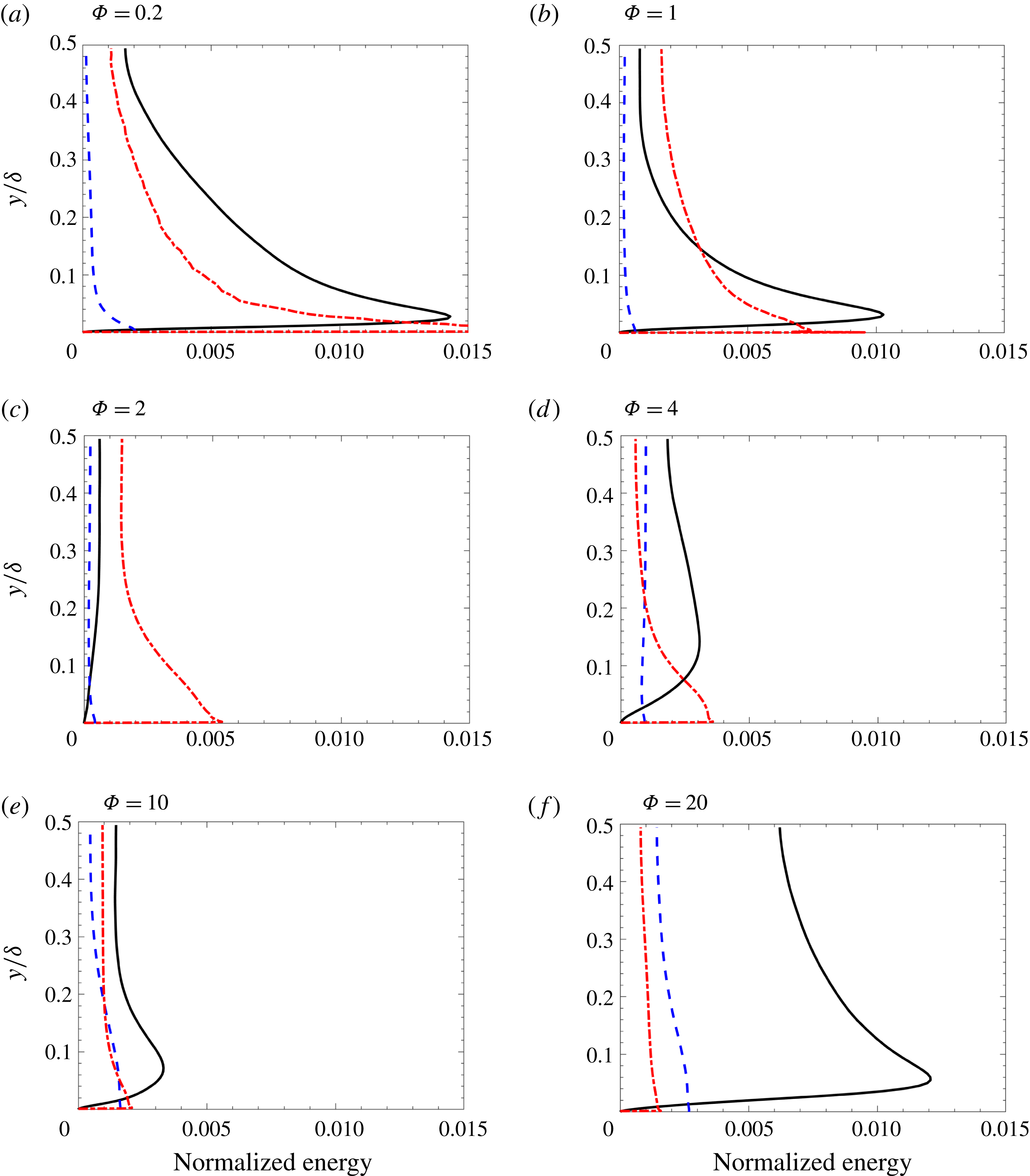
is relatively low, as seen in figure 3(b). With increasing loading, the magnitude of the drift velocity increases as seen in figure 3(d), giving rise to drag production. The resulting profiles in normalized fluid/particle energies are shown in figures 4 and 5. For the channel flows loaded with large particles, the magnitude of
 $k_{f}$
decreases with increasing
 $\unicode[STIX]{x1D6F7}$
until interphase coupling becomes strong enough at
 $\unicode[STIX]{x1D6F7}=4$
to produce significant TKE. Mass loading is also seen to affect the relative contribution to the granular energy. At low mass loading,
 $\unicode[STIX]{x1D705}$
is entirely comprised of uncorrelated motion due to the high inertia of the particles and the large normalized cluster length, such that
 $\unicode[STIX]{x1D705}\approx \langle \unicode[STIX]{x1D6E9}\rangle _{p}$
. At higher mass loading, particles begin to accumulate and fall as clusters formed near the channel walls, resulting in high values of
 $k_{p}$
. Due to the nature of the particle–wall collisions, neither
 $k_{p}$
nor
 $\langle \unicode[STIX]{x1D6E9}\rangle _{p}$
are null at the wall (Capecelatro et al.
Reference Capecelatro, Desjardins and Fox2016a
; Capecelatro, Desjardins & Fox Reference Capecelatro, Desjardins and Fox2016b
). Their relative contributions to
 $\unicode[STIX]{x1D705}$
are expected to depend on the Stokes number for decaying turbulence (Février et al.
Reference Février, Simonin and Squires2005) (i.e.
 $k_{p}/\unicode[STIX]{x1D705}$
increases with decreasing
 $St$
) and in turbulent flows generated by mean shear. For fully developed cluster-induced turbulence where the fluid-phase turbulence is produced by clusters, the Stokes number based on the fluid integral scales is constant (Capecelatro et al.
Reference Capecelatro, Desjardins and Fox2015) so that relative contributions to
 $\unicode[STIX]{x1D705}$
are nearly constant. As expected, at the channel centreline
 $k_{p}<k_{f}$
while
 $\langle \unicode[STIX]{x1D6E9}\rangle _{p}$
is produced at the channel wall due to mean slip and transported to the centreline by wall-normal fluctuations in
 $\boldsymbol{u}_{p}$
(Capecelatro et al.
Reference Capecelatro, Desjardins and Fox2016b
).
Mean two-phase statistics for
 $St_{\unicode[STIX]{x1D70F}}=0.21$
(a,b) and
 $St_{\unicode[STIX]{x1D70F}}=2.1$
(c,d) with
 $\unicode[STIX]{x1D6F7}=0.2$
(
 $\times$
),
 $\unicode[STIX]{x1D6F7}=1$
(
 $\ast$
),
 $\unicode[STIX]{x1D6F7}=2$
(○),
 $\unicode[STIX]{x1D6F7}=4$
(▵),
 $\unicode[STIX]{x1D6F7}=10$
(▫) and
 $\unicode[STIX]{x1D6F7}=20$
(♢).
Two-phase energy profiles normalized by
 $U_{b}^{2}$
for
 $St_{\unicode[STIX]{x1D70F}}=0.2$
showing
 $k_{f}$
(–),
 $k_{p}$
(– –) and
 $\langle \unicode[STIX]{x1D6E9}\rangle _{p}$
(– - – - –).
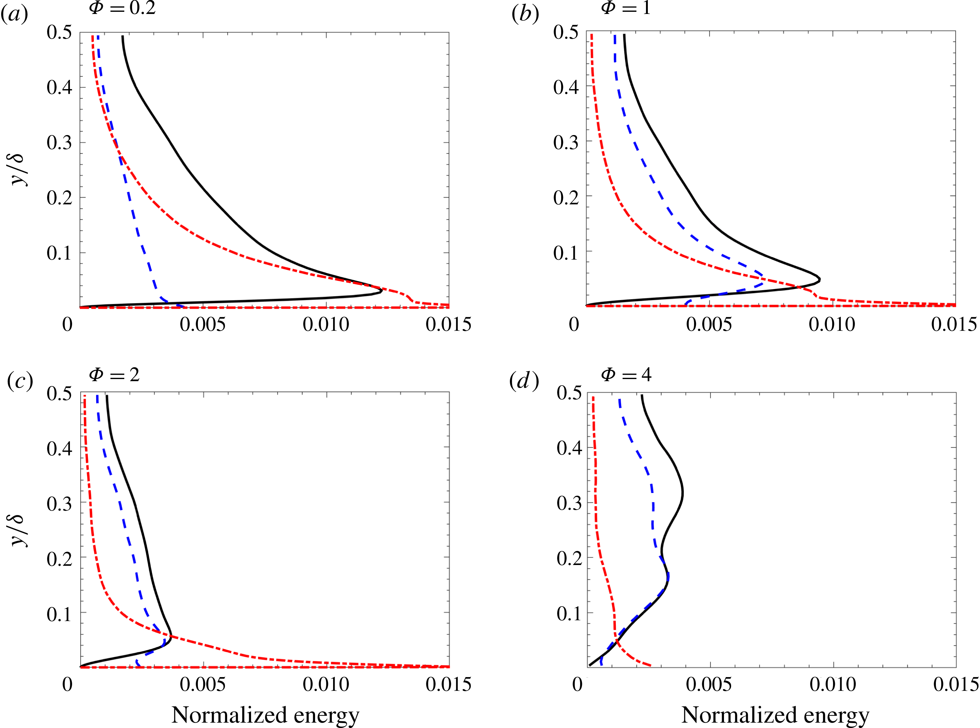
Two-phase energy profiles normalized by
 $U_{b}^{2}$
for
 $St_{\unicode[STIX]{x1D70F}}=2.1$
showing
 $k_{f}$
(–),
 $k_{p}$
(– –) and
 $\langle \unicode[STIX]{x1D6E9}\rangle _{p}$
(– - – - –).
4.3 TKE spectra
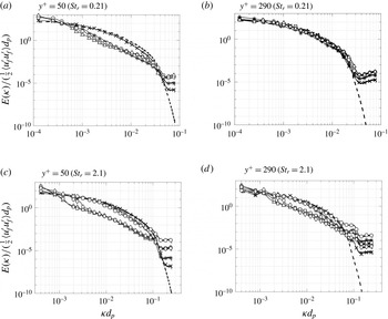
The spectral distributions of streamwise fluid-phase Reynolds stresses at the channel centreline (
 $y^{+}=290$
) and near the wall (
 $y^{+}=50$
) are shown in figure 6. In general, two-way coupling is seen to increase energy at high wavenumbers (small scales) at low mass loading, a common trend in dilute particle suspensions (Balachandar & Eaton Reference Balachandar and Eaton2010). A broadband reduction in the streamwise fluid-phase TKE is observed at high mass loading, with greater effect in the high Stokes number cases. Gualtieri et al. (Reference Gualtieri, Picano, Sardina and Casciola2013, Reference Gualtieri, Battista and Casciola2017) reported similar trends, albeit at lower mass loading, for homogeneous shear flows. In those studies, the range of scales that contribute to the Reynolds stress was found to progressively broaden with increasing mass loading. At
 $\unicode[STIX]{x1D6F7}\approx 0.8$
, momentum coupling by the particles was found to excite the Reynolds shear stress throughout the entire range of scales, similar to what is seen here. For the low Stokes number flows considered here, turbulence enhancement at small scales occurs on length scales smaller than approximately
 $14d_{p}$
, and for larger particles at scales
 ${<}4d_{p}$
. At low Stokes numbers, the inertial subrange is unaffected at the channel centreline for all values of mass loading. At
 $y^{+}=50$
a broadband reduction of TKE occurs for
 $\unicode[STIX]{x1D6F7}\geqslant 1$
. For the higher Stokes number case, broadband reduction occurs both near the wall and at the channel centreline, but only for
 $\unicode[STIX]{x1D6F7}\geqslant 4$
.
Energy spectra normalized by the corresponding streamwise fluid-phase velocity fluctuations versus normalized wavenumber
 $\unicode[STIX]{x1D705}d_{p}$
.
 $St_{\unicode[STIX]{x1D70F}}=0.21$
(a,b) and
 $St_{\unicode[STIX]{x1D70F}}=2.1$
(c,d) at
 $y^{+}=50$
(a,c) and the centreline (b,d) with
 $\unicode[STIX]{x1D6F7}=0.2$
(
 $\times$
),
 $\unicode[STIX]{x1D6F7}=1$
(*),
 $\unicode[STIX]{x1D6F7}=2$
(○),
 $\unicode[STIX]{x1D6F7}=4$
(▵),
 $\unicode[STIX]{x1D6F7}=10$
(▫) and
 $\unicode[STIX]{x1D6F7}=20$
(♢).
4.4 Fluid-phase energy budgets
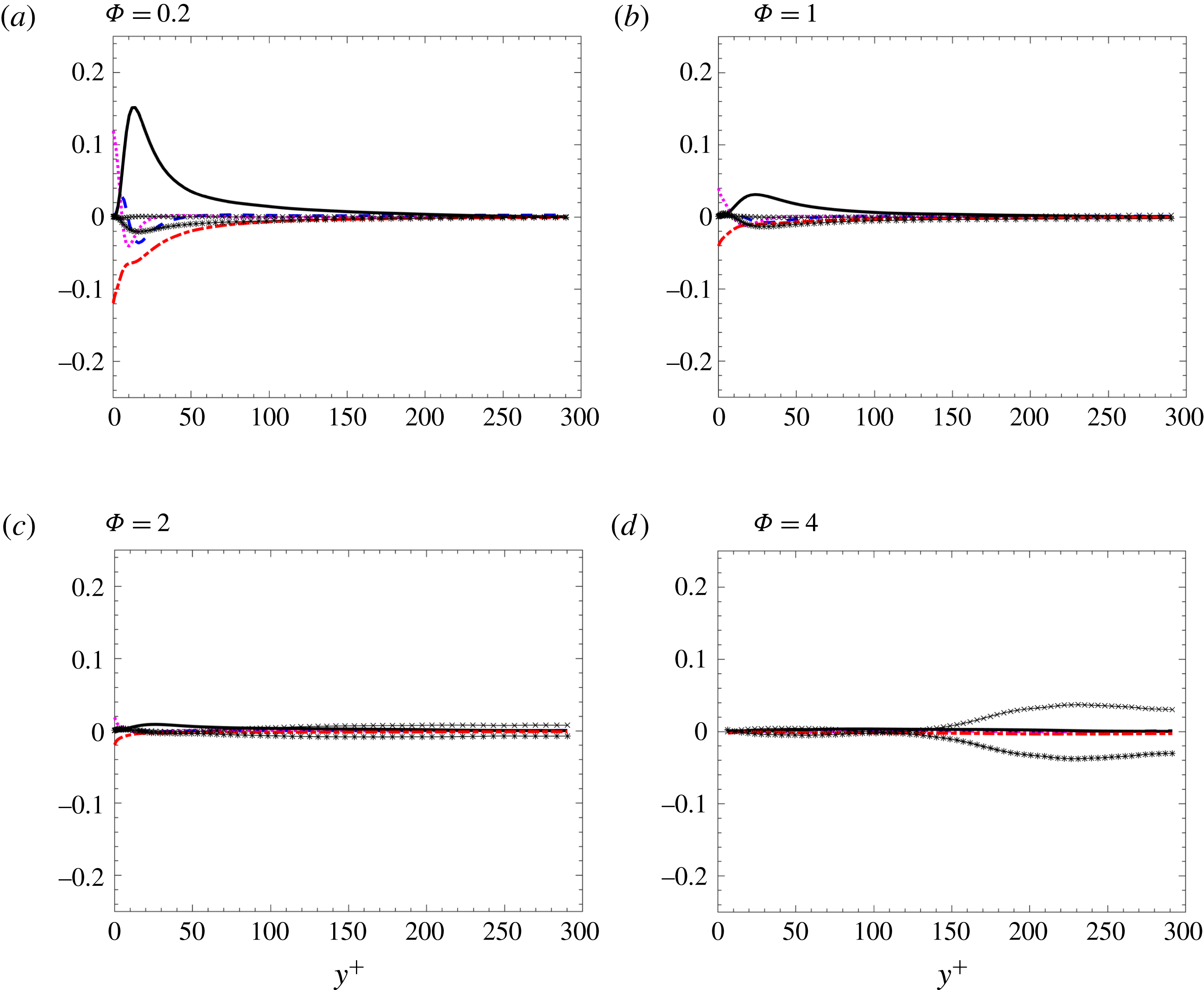
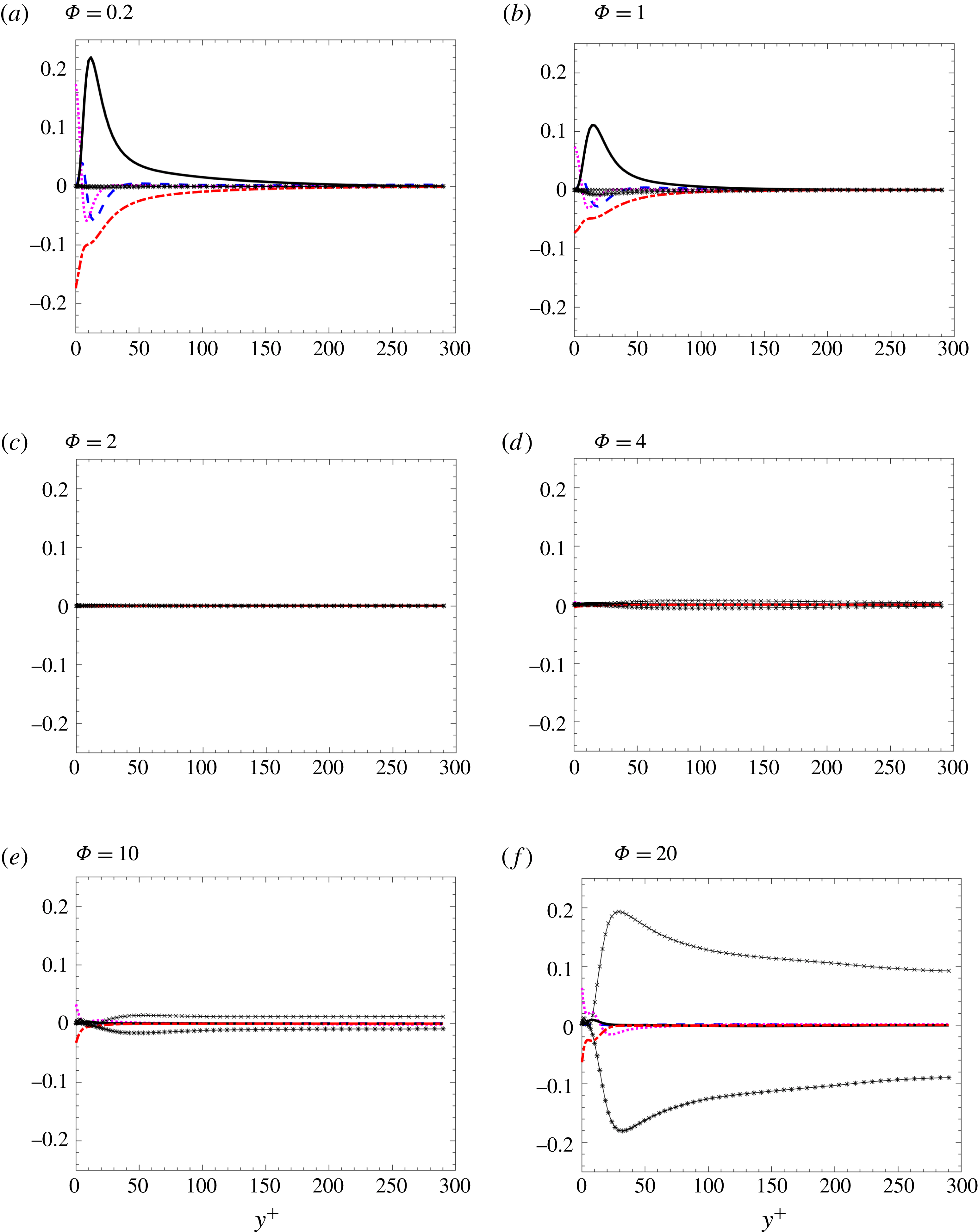
The fluid energy budgets are shown for the
 $St_{\unicode[STIX]{x1D70F}}=0.21$
cases in figure 7 and the
 $St_{\unicode[STIX]{x1D70F}}=2.1$
cases in figure 8. Three distinct regimes are identified for both particle classes. At sufficiently low mass loading (e.g.
 $\unicode[STIX]{x1D6F7}=0.2$
), the fluid-phase TKE energy budget closely resembles that of a single-phase turbulent channel, in which mean-shear production is the primary source of TKE, balanced by viscous dissipation. With increasing
 $\unicode[STIX]{x1D6F7}$
, the magnitudes of mean-shear production and viscous dissipation decrease, yet remain the dominant terms. At
 $\unicode[STIX]{x1D6F7}=2$
, mean gradients in fluid velocity have greatly diminished and the flow relaminarizes. Above
 $\unicode[STIX]{x1D6F7}=2$
, the relative contributions of drag production and exchange increase as a result of increasing drift velocity between the phases (due to the formation of clusters) as is seen in figure 3(d). At
 $\unicode[STIX]{x1D6F7}=20$
, drag production is balanced by drag exchange, with viscous dissipation only contributing very near the wall. Unlike in the low-mass-loading regime, energy is being produced throughout the channel for
 $\unicode[STIX]{x1D6F7}>2$
.
The transition between turbulence regimes is seen to occur faster in the lower Stokes number case. At low mass loading, the lower Stokes number flows are more effective at dissipating fluid-phase TKE. Recall that the drag-dissipation-and-exchange rate (2.14) is proportional to the spatially correlated particle-phase velocity fluctuations
 $\boldsymbol{u}_{p}^{\prime \prime }$
. Because the uncorrelated granular motion arises when particles deviate from fluid streamlines (e.g. due to particle trajectory crossings), the lower Stokes number particles exhibit higher correlated energy and thus larger values of
 ${\mathcal{D}}{\mathcal{E}}$
. While all the terms appearing in the fluid-phase energy budget are approximately null at
 $\unicode[STIX]{x1D6F7}=2$
for both particle sizes, the interphase coupling terms (
 ${\mathcal{D}}{\mathcal{P}}$
and
 ${\mathcal{D}}{\mathcal{E}}$
) are non-negligible at
 $\unicode[STIX]{x1D6F7}=4$
for the channel seeded with smaller particles, while all the terms remain relatively small for the channel seeded with larger particles.
Fluid-phase TKE budget normalized by viscous scales
 $u_{\unicode[STIX]{x1D70F}}^{4}/\unicode[STIX]{x1D708}$
for
 $St_{\unicode[STIX]{x1D70F}}=0.21$
. Turbulent convection (– –),
 $-\unicode[STIX]{x1D700}$
(– - – - –),
 $\text{d}{\mathcal{E}}/\text{d}y$
(
 $\cdots \,$
),
 ${\mathcal{P}}_{shear}$
(–),
 ${\mathcal{D}}{\mathcal{P}}$
(–
 $\times$
–) and
 ${\mathcal{D}}{\mathcal{E}}$
(–
 $\ast$
–).
Fluid-phase TKE budget normalized by viscous scales
 $u_{\unicode[STIX]{x1D70F}}^{4}/\unicode[STIX]{x1D708}$
for
 $St_{\unicode[STIX]{x1D70F}}=2.1$
. Turbulent convection (–),
 $-\unicode[STIX]{x1D700}$
(– - – - –),
 $\text{d}{\mathcal{E}}/\text{d}y$
(
 $\cdots$
),
 ${\mathcal{P}}_{shear}$
(–),
 ${\mathcal{D}}{\mathcal{P}}$
(–
 $\times$
–) and
 ${\mathcal{D}}{\mathcal{E}}$
(–
 $\ast$
–).
4.5 Where does the energy go?
We have seen up to this point that increasing particle loading in an initially unladen channel flow will reduce fluid-phase TKE until the mass loading is high enough for drag production to contribute. As was seen in figures 7 and 8, the level of reduction is tied to both the mean mass loading and Stokes number. Yet it remains to be seen how the energy is transferred between phases and ultimately dissipated to heat the fluid. In our previous work (Capecelatro et al.
Reference Capecelatro, Desjardins and Fox2015) we showed that in homogeneous (unbounded) gas–solid flows in which mean gradients are null, mean kinetic energy produced by particles settling under gravity is balanced by mean drag, which generates viscous heating of the fluid. In the presence of clusters, drag production produces fluid-phase TKE that is eventually dissipated to heat the fluid. The route to fluid heating occurs (i) directly by viscous dissipation resulting from resolved small-scale velocity fluctuations in the fluid phase (
 $\unicode[STIX]{x1D700}$
) and (ii) indirectly by viscous dissipation of unresolved fluid velocity fluctuations, e.g. in the viscous boundary layer around individual particles. The remaining fraction of the fluid-phase TKE is transferred to the particle phase by drag exchange (
 ${\mathcal{D}}{\mathcal{E}}$
) and ultimately dissipated to heat the fluid through fluctuating drag.
In order to analyse the mechanisms responsible for fluid-phase dissipation in the channel flows considered here, we must introduce the averaged particle-phase equations of motion. The transport of particle-phase TKE is given by
 $$\begin{eqnarray}\displaystyle \frac{1}{\langle \unicode[STIX]{x1D6FC}_{p}\rangle }\frac{\text{d}}{\text{d}y}\left(\frac{1}{2}\langle \unicode[STIX]{x1D6FC}_{p}\rangle \langle v_{p}^{\prime \prime }\boldsymbol{u}_{p}^{\prime \prime }\boldsymbol{\cdot }\boldsymbol{u}_{p}^{\prime \prime }\rangle _{p}+{\mathcal{E}}_{p}\right)={\mathcal{P}}_{p}-\unicode[STIX]{x1D700}_{p}+{\mathcal{D}}{\mathcal{E}}_{p}, & & \displaystyle\end{eqnarray}$$
where
 ${\mathcal{E}}_{p}=\langle \unicode[STIX]{x1D64B}_{p,y}\boldsymbol{\cdot }\boldsymbol{u}_{p}^{\prime \prime }\rangle _{p}$
, with
 $\unicode[STIX]{x1D64B}_{p}$
the particle-phase pressure tensor that contains the uncorrelated granular energy and whose trace is the granular temperature
 $\langle \unicode[STIX]{x1D6E9}\rangle _{p}$
. The particle-phase dissipation rate is given by
 $$\begin{eqnarray}\displaystyle & \displaystyle \unicode[STIX]{x1D700}_{p}=\langle \unicode[STIX]{x1D64B}_{p}\boldsymbol{ : }\unicode[STIX]{x1D735}\boldsymbol{u}_{p}^{\prime \prime }\rangle _{p}-\langle \unicode[STIX]{x1D6E9}\unicode[STIX]{x1D735}\boldsymbol{\cdot }\boldsymbol{u}_{p}^{\prime \prime }\rangle _{p} & \displaystyle\end{eqnarray}$$
and
 ${\mathcal{P}}_{p}=-\langle u_{p}^{\prime \prime }v_{p}^{\prime \prime }\rangle _{p}~\text{d}\langle u_{p}\rangle _{p}/\text{d}y$
is the only mechanism by which
 $k_{p}$
is generated. Finally, the particle-phase drag-dissipation-and-exchange rate is
 $$\begin{eqnarray}\displaystyle & \displaystyle {\mathcal{D}}{\mathcal{E}}_{p}=\frac{1}{\unicode[STIX]{x1D70F}_{p}}\left(\langle \boldsymbol{u}_{f}^{\prime \prime \prime }\boldsymbol{\cdot }\boldsymbol{u}_{p}^{\prime \prime }\rangle _{p}-\langle \boldsymbol{u}_{p}^{\prime \prime }\boldsymbol{\cdot }\boldsymbol{u}_{p}^{\prime \prime }\rangle _{p}\right), & \displaystyle\end{eqnarray}$$
and is the only source of
 $k_{p}$
in the absence of mean shear. To close the set of equations, a transport equation for the averaged particle-phase pressure tensor is needed, which is given by
 $$\begin{eqnarray}\displaystyle \frac{1}{\langle \unicode[STIX]{x1D6FC}_{p}\rangle }{\displaystyle \frac{\text{d}}{\text{d}y}}\left({\displaystyle \frac{1}{2}}\langle \unicode[STIX]{x1D6FC}_{p}\rangle \langle v_{p}^{\prime \prime }\unicode[STIX]{x1D64B}_{y}\rangle _{p}+\langle \unicode[STIX]{x1D64C}_{y}\rangle _{p}\right)=\boldsymbol{{\mathcal{P}}}_{P}+\unicode[STIX]{x1D73A}_{p}-{\displaystyle \frac{2}{\unicode[STIX]{x1D70F}_{p}}}\langle \unicode[STIX]{x1D64B}\rangle _{p}+\boldsymbol{{\mathcal{C}}}, & & \displaystyle\end{eqnarray}$$
where
 $\unicode[STIX]{x1D64C}_{y}$
is the wall-normal component of the granular-flux tensor (Jenkins & Savage Reference Jenkins and Savage1983),
 $\boldsymbol{{\mathcal{C}}}$
is the collisional dissipation rate proportional to the coefficient of restitution (Passalacqua et al.
Reference Passalacqua, Galvin, Vedula, Hrenya and Fox2011) and
 $\boldsymbol{{\mathcal{P}}}_{P}$
represents mean-shear production of granular pressure (Capecelatro et al.
Reference Capecelatro, Desjardins and Fox2016a
). In summary, the particle phase exchanges energy with the fluid via
 ${\mathcal{D}}{\mathcal{E}}_{p}$
, and dissipation of particle-phase Reynolds stresses,
 $\unicode[STIX]{x1D73A}_{p}$
, appears as the principal production term for
 $\langle \unicode[STIX]{x1D64B}_{p}\rangle _{p}$
. The main role of
 $\boldsymbol{{\mathcal{C}}}$
in (4.5) is to drive
 $\langle \unicode[STIX]{x1D64B}\rangle _{p}$
towards isotropy.
(a) Channel-averaged dissipation based on the mixture density
 $\unicode[STIX]{x1D70C}_{f}\unicode[STIX]{x1D6FC}_{f}+\unicode[STIX]{x1D70C}_{p}\unicode[STIX]{x1D6FC}_{p}$
normalized by viscous scales
 $u_{\unicode[STIX]{x1D70F}}^{4}/\unicode[STIX]{x1D708}$
for (a)
 $St_{\unicode[STIX]{x1D70F}}=0.21$
and (b)
 $St_{\unicode[STIX]{x1D70F}}=2.1$
.
 $\overline{{\mathcal{D}}{\mathcal{E}}}$
(○),
 $\overline{{\mathcal{D}}{\mathcal{E}}_{p}}$
(♢),
 $-\overline{\unicode[STIX]{x1D700}}$
(▫), and
 $-\overline{\unicode[STIX]{x1D700}_{p}}$
(▵),
 $\overline{{\mathcal{C}}}$
(▿).
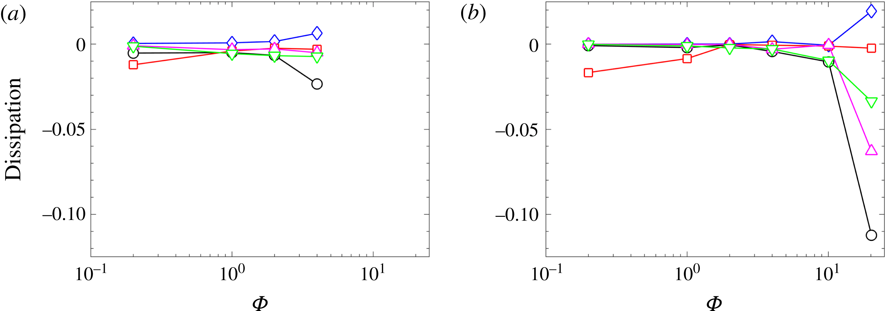
The channel-averaged dissipation terms are shown in figure 9 as a function of mass loading for both particle sizes. Here, the overbar denotes a volume-average quantity weighted on
 $\unicode[STIX]{x1D6FC}_{f}$
and
 $\unicode[STIX]{x1D6FC}_{p}$
for terms appearing in the fluid-phase and particle-phase equations, respectively, such that the sum contributes to the total dissipation based on the mixture density
 $\unicode[STIX]{x1D70C}_{m}$
. In the limit
 $\unicode[STIX]{x1D6F7}$
approaches zero (i.e. approaching a single-phase channel), dissipation is entirely due to
 $\unicode[STIX]{x1D700}$
. At
 $\unicode[STIX]{x1D6F7}=0.2$
, dissipation in the channel loaded with large particles (
 $St_{\unicode[STIX]{x1D70F}}=2.1$
) is almost entirely due to
 $\unicode[STIX]{x1D700}$
. Due to the larger correlated motion attributed to the smaller particles (as seen by the finite contribution of
 $k_{p}$
in figure 4),
 ${\mathcal{D}}{\mathcal{E}}$
plays a role in dissipating TKE for
 $St_{\unicode[STIX]{x1D70F}}=0.21$
as low as
 $\unicode[STIX]{x1D6F7}=0.2$
. As a result, the TKE budget for the smaller particles appears to transition faster from a single-phase flow dominated by mean-shear production to cluster-induced turbulence (CIT), as was seen in figures 7 and 8. In the high mass loading limit,
 $\unicode[STIX]{x1D700}$
is null and the drag exchange terms in each phase,
 ${\mathcal{D}}{\mathcal{E}}$
and
 ${\mathcal{D}}{\mathcal{E}}_{p}$
dominate. The collisional dissipation is seen to only contribute above
 $\unicode[STIX]{x1D6F7}\geqslant 10$
, corresponding to a mean volume fraction
 $\overline{\unicode[STIX]{x1D6FC}}_{p}\geqslant 5\times 10^{-3}$
.
In summary, at relatively low mass loading (
 $\unicode[STIX]{x1D6F7}<2$
) viscous dissipation resulting from small-scale velocity fluctuations is the primary mechanism responsible for energy loss. Within this regime, higher levels of correlated energy (
 $k_{p}$
) in the low Stokes number flows results in finite (but still small) energy transfer from the particle phase to the fluid via
 ${\mathcal{D}}{\mathcal{E}}_{p}$
. Because the channel wall separation
 $2\unicode[STIX]{x1D6FF}<{\mathcal{L}}$
for the larger particle cases, higher levels of uncorrelated granular energy (
 $\langle \unicode[STIX]{x1D6E9}\rangle _{p}$
) prevent energy transfer from the particle phase to the fluid until the mass loading is sufficiently high and the spontaneous generation of clusters generates
 $k_{p}$
. At high mass loading (
 $\unicode[STIX]{x1D6F7}=10$
), dissipation is entirely due to energy transfer between the phases and collisions.
5 Concluding remarks
In this work, we present results of vertical turbulent particle-laden channel flows using fully coupled Eulerian–Lagrangian simulations. A transition in turbulence-generation mechanisms is observed going from low to high particle loading. Three distinct regimes are identified based on the mean mass loading: (i) weak interphase coupling at low mass loading (
 $\unicode[STIX]{x1D6F7}\leqslant 1$
) wherein mean-shear production is the dominant mechanism for generating fluid-phase TKE; (ii) moderate coupling at intermediate mass loadings (
 $2\leqslant \unicode[STIX]{x1D6F7}\leqslant 4$
) in which the flow relaminarizes; and (iii) strong interphase coupling at high mass loading (
 $\unicode[STIX]{x1D6F7}\geqslant 10$
) where the fluid-phase TKE is entirely generated by mean interphase slip velocities, termed drag production, and balanced by a drag exchange term. Remarkably, the different turbulence production mechanisms in regimes (i) and (iii) exhibit essentially no overlap, resulting from the near absence of fluid-phase turbulence in regime (ii). In addition, for a large Stokes number (
 $St_{\unicode[STIX]{x1D6FF}}=17.86$
), we show that the components of particle-phase granular energy contribute differently in each regime. At low particle loading, granular energy is entirely comprised of spatially uncorrelated motion due to the finite inertia of the particles, resulting in high granular temperature. At high mass loading, clusters spontaneously form and fall near the channel wall, resulting in large contributions of spatially correlated particle-phase TKE. Despite the seeming simplicity of a turbulent channel flow, the results reported here demonstrate the complex behaviour of disperse two-phase flows across granular regimes and point to two key components that must be accounted for in future modelling efforts. First, predictive models should correctly decompose the spatially correlated and uncorrelated components of granular energy as they play fundamentally different roles in the regimes identified. Second, accurate models of the drift velocity are needed to correctly predict drag production that plays a key role in the transition in turbulence regimes.
Acknowledgements
We would like to acknowledge high-performance computing support from the Advanced Research Computing Technology Services at the University of Michigan. O.D. and R.O.F. gratefully acknowledge support from the US National Science Foundation under grants CBET-1437865 and CBET-1437903.
Appendix A. The role of nonlinear drag
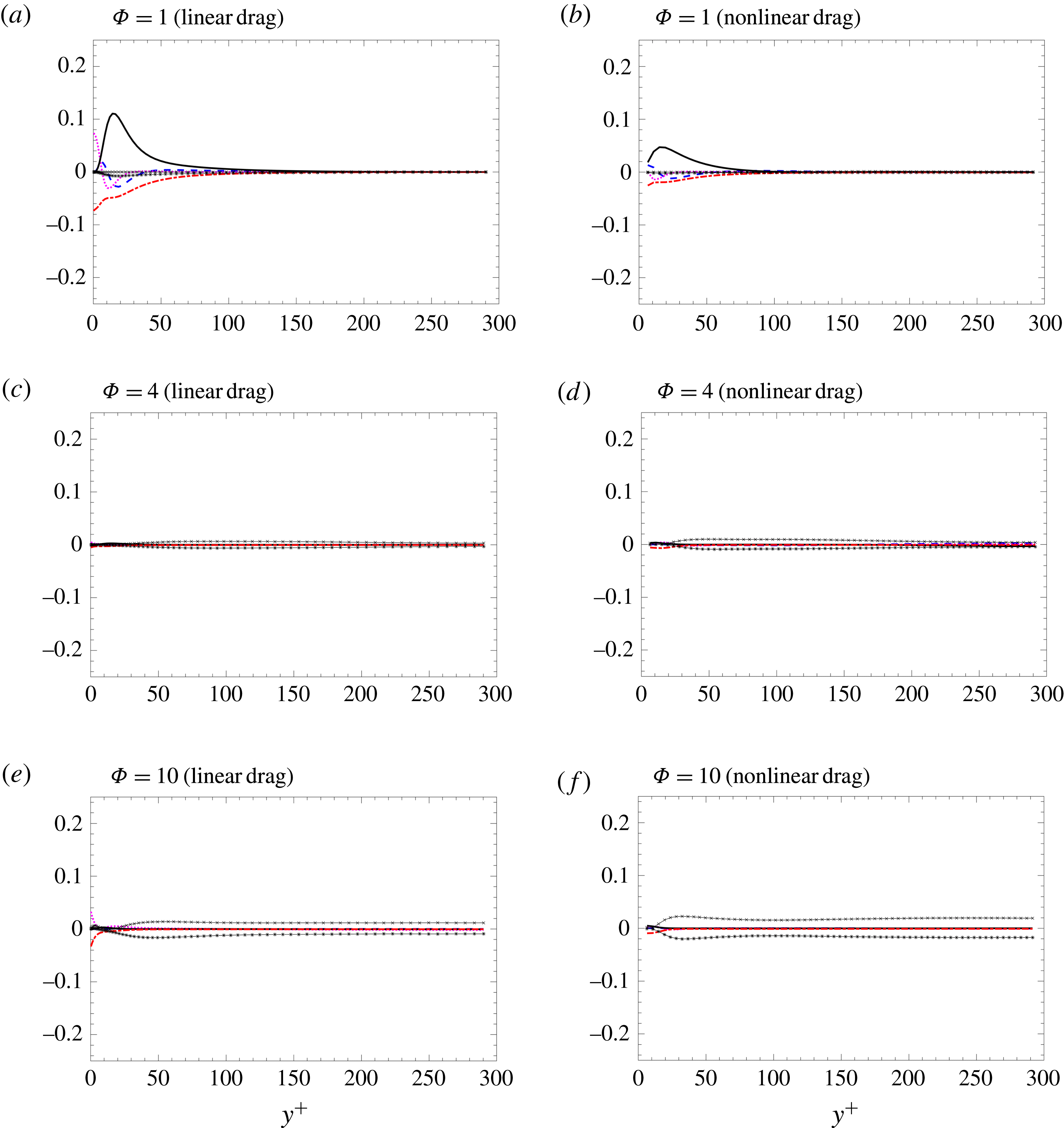
In real systems with moderate Reynolds numbers and particle volume fractions, particles will experience drag with a nonlinear dependence on volume fraction and velocity (see, e.g., Tenneti, Garg & Subramaniam Reference Tenneti, Garg and Subramaniam2011). In the present manuscript linear Stokes drag was considered to simplify the Reynolds-average analysis. Here we assess the importance of the higher-order terms. Figure 10 shows fluid-phase TKE energy budgets for
 $St_{\unicode[STIX]{x1D70F}}=2.1$
with
 $1\leqslant \unicode[STIX]{x1D6F7}\leqslant 10$
using the nonlinear drag correlation of Tenneti et al. (Reference Tenneti, Garg and Subramaniam2011), given by
 $$\begin{eqnarray}\displaystyle & \displaystyle \boldsymbol{F}_{drag}^{(i)}=\boldsymbol{F}_{s}^{(i)}\left({\displaystyle \frac{1+0.15Re_{p}^{0.687}}{\unicode[STIX]{x1D6FC}_{f}^{2}}}+\unicode[STIX]{x1D6FC}_{f}F_{1}(\unicode[STIX]{x1D6FC}_{f})+\unicode[STIX]{x1D6FC}_{f}F_{2}(\unicode[STIX]{x1D6FC}_{f},\,Re_{p})\right), & \displaystyle\end{eqnarray}$$
where
 $\boldsymbol{F}_{s}^{(i)}=(\boldsymbol{u}_{f}[\boldsymbol{x}_{p}^{(i)}]-\boldsymbol{v}_{p}^{(i)})/\unicode[STIX]{x1D70F}_{p}$
is the Stokes drag contribution for particle ‘
 $i$
’ used in (2.2),
 $F_{1}(\unicode[STIX]{x1D6FC}_{f})=5.81\unicode[STIX]{x1D6FC}_{p}/\unicode[STIX]{x1D6FC}_{f}^{3}+0.48\unicode[STIX]{x1D6FC}_{p}^{1/3}/\unicode[STIX]{x1D6FC}_{f}^{4}$
, and
 $F_{2}(\unicode[STIX]{x1D6FC}_{f},\,Re_{p})=\unicode[STIX]{x1D6FC}_{p}^{3}Re_{p}(0.95+0.61\unicode[STIX]{x1D6FC}_{p}^{3}/\unicode[STIX]{x1D6FC}_{f}^{2})$
. Due to the nonlinear contributions from
 $\unicode[STIX]{x1D6FC}_{f}$
and
 $Re_{p}$
, phase averaging the drag contribution becomes cumbersome. Instead, the total drag can be decomposed into mean and fluctuating components via
 $$\begin{eqnarray}\displaystyle \boldsymbol{F}_{drag}^{(i)}=\left\langle \boldsymbol{F}_{drag}\right\rangle +\boldsymbol{F}_{drag}^{\prime }, & & \displaystyle\end{eqnarray}$$
where
 $\langle \boldsymbol{F}_{drag}\rangle$
is defined according to (A 1) using averaged quantities (e.g.
 $\langle \unicode[STIX]{x1D6FC}_{f}\rangle$
,
 $\langle \boldsymbol{u}_{f}\rangle _{f}$
, etc.), and
 $\boldsymbol{F}_{drag}^{\prime }=\boldsymbol{F}_{drag}-\langle \boldsymbol{F}_{drag}\rangle$
represents the difference.
Although the nonlinear drag is seen to impact the magnitude of the terms appearing in the TKE balance, overall the same trend is observed. At low mass loading, mean-shear production is dominated by viscous dissipation, and drag coupling terms have minimal effect. At intermediate values of mass loading (
 $\unicode[STIX]{x1D6F7}=4$
) similar relaminarization is observed, and at high mass loading (
 $\unicode[STIX]{x1D6F7}=10$
) drag production is entirely balanced by drag exchange. We note that nonlinear contributions to drag do indeed have meaningful impact on the wall-normal profiles of mean volume fraction interphase slip velocity. Nonetheless, we expect real systems to undergo a similar transition from the dilute limit where classical mean-shear production is primarily responsible for generating fluid-phase TKE to high-mass-loading suspensions dominated by drag production. It is likely that Reynolds number effects on the drag law are masked at high mass loading by other near-field interactions, and thus in general these higher-order terms should be accounted for.
Fluid-phase TKE budget normalized by viscous scales
 $u_{\unicode[STIX]{x1D70F}}^{4}/\unicode[STIX]{x1D708}$
for
 $St_{\unicode[STIX]{x1D70F}}=2.1$
with linear Stokes drag (a,c,e) and the nonlinear drag correlation given by Tenneti et al. (Reference Tenneti, Garg and Subramaniam2011) (b,d,f). Turbulent convection (– –),
 $-\unicode[STIX]{x1D700}$
(– - – - –),
 $\text{d}{\mathcal{E}}/\text{d}y$
(
 $\cdots$
),
 ${\mathcal{P}}_{shear}$
(–),
 ${\mathcal{D}}{\mathcal{P}}$
(–
 $\times$
–) and
 ${\mathcal{D}}{\mathcal{E}}$
(–
 $\ast$
–).