1 Introduction
Descriptions of turbulent wall-flow statistical profiles employ a variety of approaches. These often use distance from the wall scaling (Townsend Reference Townsend1976; Perry & Chong Reference Perry and Chong1982; Marusic & Kunkel Reference Marusic and Kunkel2003), or, to the extent possible, adopt analytical methods that employ matched asymptotic expansions (Millikan Reference Millikan1939; Mellor Reference Mellor1972; Panton Reference Panton2005). Such approaches yield useful formulas describing portions of the mean velocity profile, and in some instances profiles of the velocity variances and their higher statistical moments.
Similar successes derive from a more recently developed analysis framework (Wei et al.
Reference Wei, Fife, Klewicki and McMurtry2005; Fife, Klewicki & Wei Reference Fife, Klewicki and Wei2009; Klewicki Reference Klewicki2013b
), that has also been useful in connecting observed flow field properties to the structure of the mean momentum equation, and to the underlying flow physics (Klewicki, Fife & Wei Reference Klewicki, Fife and Wei2007; Klewicki et al.
Reference Klewicki, Philip, Marusic, Chauhan and Morrill-Winter2014). This approach involves analysis of the leading-order forms of the mean momentum equation that apply to different subdomains between the wall at
 $y=0$
, and the channel or pipe centreline or boundary layer edge at
 $y=\unicode[STIX]{x1D6FF}$
. The analytical treatment is simpler and more precise for pipes and channel than for boundary layers. This stems from the mean momentum balance (MMB) for pipes and channels having a pressure gradient term that does not depend on
 $y$
. The MMB for the zero-pressure gradient turbulent boundary layer (TBL) is
 $$\begin{eqnarray}\underbrace{\frac{\unicode[STIX]{x2202}^{2}U^{+}}{\unicode[STIX]{x2202}y^{+2}}}_{VF}+\underbrace{\frac{\unicode[STIX]{x2202}T^{+}}{\unicode[STIX]{x2202}y^{+}}}_{TI}+\underbrace{\overline{A}^{+}}_{MI}=0.\end{eqnarray}$$
In (1.1)
 $T^{+}=\langle -uv\rangle ^{+}$
,
 $\overline{A}^{+}=-[U^{+}(\unicode[STIX]{x2202}U^{+}/\unicode[STIX]{x2202}x^{+})+V^{+}(\unicode[STIX]{x2202}U^{+}/\unicode[STIX]{x2202}y^{+})]$
(note
 $\overline{A}$
is the mean advection or mean inertia, MI) and a superscript
 $+$
denotes viscous normalization. Herein we employ the friction Reynolds number,
 $\unicode[STIX]{x1D6FF}^{+}=\unicode[STIX]{x1D6FF}u_{\unicode[STIX]{x1D70F}}/\unicode[STIX]{x1D708}$
, where
 $u_{\unicode[STIX]{x1D70F}}=\sqrt{\unicode[STIX]{x1D70F}_{wall}/\unicode[STIX]{x1D70C}}$
is the friction velocity and
 $\unicode[STIX]{x1D708}$
is the kinematic viscosity. In the case of pipes/channel the last term in (1.1) is replaced by the constant term
 $1/\unicode[STIX]{x1D6FF}^{+}$
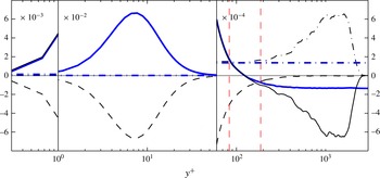
. Also, see the thin (black) lines in figure 3, which provides an example of the wall-normal distribution of the three terms in (1.1).
The wall-normal variation of
 $\overline{A}^{+}$
in (1.1) complicates both hypothesis based scaling arguments, as well as analytical treatments that employ the appropriately simplified form of the mean momentum equation. For example, George and coworkers (e.g. George & Castillo Reference George and Castillo1997; George Reference George2007) found that analyses employing their asymptotic invariance principle (AIP) indicate that within pipe or channel flows there is a domain over which the mean velocity profile asymptotically adheres to a logarithmic variation with distance from the wall. For the boundary layer, however, they found that the mean velocity variation on the relevant domain adheres to a power law, and further surmised that the correct velocity scale on this domain is the free-stream velocity,
 $U_{\infty }$
, rather than the friction velocity,
 $u_{\unicode[STIX]{x1D70F}}$
(George & Castillo Reference George and Castillo1997; George Reference George2007). The analysis of Jones, Nickels & Marusic (Reference Jones, Nickels and Marusic2008) provides an important contribution regarding the question of appropriate velocity scale. Specifically, they clarified that, independent of AIP validity, the mean momentum equation also asymptotically admits a self-similar form when
 $u_{\unicode[STIX]{x1D70F}}$
is used as the velocity scale. Within the context of the present analysis framework, Klewicki (Reference Klewicki2013b
) provided evidence that the MMB for the boundary layer admits the same type of self-similar structure as in channels and pipes. Owing, however, to the non-constancy of
 $\overline{A}^{+}$
across the outer region of the flow, this conclusion was only founded on order of magnitude estimates. More recently, Talluru et al. (Reference Talluru, Djenidi, Kamruzzaman and Antonia2016) provided an analysis of the mean boundary layer equation that explored the conditions for self-preserving (self-similar) solutions. Relative to the smooth flat plate case, they conclude that a self-preserving solution is not possible across the entire layer. Here we note, however, that while Talluru et al. (Reference Talluru, Djenidi, Kamruzzaman and Antonia2016) employed a leading-order reduction to arrive at the mean boundary layer equation, they did not leverage the fact that at any given streamwise location the leading balances of terms in this equation also vary according to established scaling relationships with wall-normal distance (Wei et al.
Reference Wei, Fife, Klewicki and McMurtry2005).
The present analysis framework exploits the layered structure of leading balances in the MMB across the layer. The asymptotic emergence of an exactly logarithmic mean profile follows from such an analysis of pipe or channel flow, as does the
 $y^{+}$
location of maximum
 $\langle -uv\rangle$
varying like
 $\sqrt{\unicode[STIX]{x1D6FF}^{+}}$
. Owing to the
 $y$
dependence of
 $\overline{A}^{+}$
, however, similarly precise analyses have not been possible for the TBL. Thus, even though the existence of a log-region in pipes and channels is well accepted, the analytical case for an asymptotically logarithmic mean profile in the TBL is less well founded (e.g. George Reference George2007; Klewicki Reference Klewicki2013b
). As such, the central aim of this paper is to evidence that, indeed (1.1) can be recast such that
 $\overline{A}^{+}$
is replaced by a term that is constant in
 $y$
for any given
 $\unicode[STIX]{x1D6FF}^{+}$
. The theoretical implications of this are significant, as it indicates that MMB based predictions for an asymptotically logarithmic mean profile, the peak location of
 $T^{+}$
, and the wall-normal location of the log-region in the TBL are on the same analytical footing as for the pipe or channel. The data analyses herein make use of high resolution measurements up to a
 $\unicode[STIX]{x1D6FF}^{+}$
of 16 400 (with
 $\unicode[STIX]{x1D6FF}$
based on the ‘composite’ fit of Chauhan, Monkewitz & Nagib (Reference Chauhan, Monkewitz and Nagib2009), or
 $\unicode[STIX]{x1D6FF}_{99}^{+}$
of 12 500 based on the location of 99 % of mean velocity), that is considerably higher than previous investigations. Also, whenever possible we also employ the mean velocity and Reynolds shear stress distributions from the boundary layer direct numerical simulation (DNS) database of Sillero, Jiménez & Moser (Reference Sillero, Jiménez and Moser2013).
1.1 Structure of the boundary layer based on the mean momentum equation
Both analytical and empirical considerations of the mean momentum equation in the canonical wall flows indicate that each flow exhibits an apparent layered structure (e.g. Wei et al.
Reference Wei, Fife, Klewicki and McMurtry2005; Fife et al.
Reference Fife, Klewicki and Wei2009). The three term balance in channel and pipe flows features the mean viscous force (VF), the net effect of turbulent inertia (TI) and a mean pressure gradient force (PG), i.e. VF + TI + PG = 0 (cf. (1.1)). For the boundary layer, there is also a three term balance, but relative to the channel/pipe flow equation the PG term is replaced by the inertia of the mean flow (
 $\overline{A}$
). For a detailed description of the balance of terms, we refer the reader to Wei et al. (Reference Wei, Fife, Klewicki and McMurtry2005) and Klewicki (Reference Klewicki2013a
).
Previous investigations provide clear evidence that the momentum balance scaling layers in channels, pipes, and boundary layers exhibit the same order of magnitude Reynolds number dependencies (e.g. Wei et al.
Reference Wei, Fife, Klewicki and McMurtry2005; Klewicki Reference Klewicki2013a
). The fact that the channel and pipe momentum equations can be written in identical forms is, however, a good reason to suspect that at least some of the
 $\unicode[STIX]{x1D6FF}^{+}$
dependencies associated with their respective layer structure will approach the same functions at high Reynolds number. Evidence from high Reynolds number pipe and boundary layer data suggest that the von Kármán constant attains the same value on the inertial sublayer (Marusic et al.
Reference Marusic, Monty, Hultmark and Smits2013).
It is rational to suspect that the physical origin of the noted differences in pipes, channels and boundary layers are connected to the different outer boundary condition on the boundary layer flow, which, for example, underlies the more rapid growth of boundary layer displacement thickness (centroid of mean vorticity, Lighthill Reference Lighthill1958), especially near the onset of the four layer regime (Klewicki Reference Klewicki2013a
). In the present context, such physics are manifest in the above noted differences between the PG and
 $\overline{A}$
terms in the outer portion of channels and boundary layers, respectively. For the flat plate boundary layer, Klewicki (Reference Klewicki2013b
) borrowed from the pressure gradient boundary layer analysis of Metzger, Lyons & Fife (Reference Metzger, Lyons and Fife2008) to demonstrate that, on the inertial domain, the boundary layer equations nominally exhibit the same type of self-similar behaviour as in channels and pipes. This conclusion, however, remained ambiguous owing the variation of
 $\overline{A}^{+}$
with
 $y^{+}$
.
The analysis provided herein evidences that equivalent but transformed versions of the mean and turbulent advection terms in (1.1) can be cast in an invariant form that effectively removes the
 $y^{+}$
dependence of
 $\overline{A}^{+}$
. Numerous data comparisons are used to validate the analytically predicted structure of the physically realized solution to (1.1). This includes evidence that the similarity structure admitted by the boundary layer equation is indeed the same as that admitted by the channel (or pipe) MMB. An important ramification of this is the expectation that all three of the canonical flows asymptotically adhere to a logarithmic mean profile.
1.2 Organization of the rest of the paper
The rest of this paper is organized in the following manner. Section 2 presents details of the experimental and DNS databases that are employed. Rather than presenting the full theoretical analysis at first and subsequently the experimental evidence, from § 3 onwards we have are interspersed theory with the experimental evidences to support any assumptions made in the theory and to verify the predictions. The main aim of § 3 is to eliminate the
 $y$
-dependence of the
 $\overline{A}$
term, and subsequently the
 $y$
-dependence of the TI term on the inertial domain. Upon attaining this aim, one can carry out an analysis similar to that of Wei et al. (Reference Wei, Fife, Klewicki and McMurtry2005) and Fife et al. (Reference Fife, Wei, Klewicki and McMurtry2005b
) (which is applicable to channel or pipe flows where the last term in the MMB equation is
 $1/\unicode[STIX]{x1D6FF}^{+}$
). This treatment is taken up for the transformed boundary layer equation in §§ 4 and 5. In § 4, we analyse the scaling behaviour of the ‘intermediate region’, where the three terms in the MMB equation are of equal order of magnitude. This allows us to surmise
 $\unicode[STIX]{x1D6FF}^{+}$
-invariant bounds of the intermediate region, and predict that the peak location of
 $\langle -uv\rangle$
varies like
 $\sqrt{\unicode[STIX]{x1D6FF}^{+}}$
. We extend the scaling of the intermediate region to a ‘hierarchical’ scaling analysis in § 5. Among other things, here we define a self-similar length scale distribution for momentum transport in turbulent boundary layers. This description employs derivatives of the terms in the MMB equation; yielding an
 $O(1)$
self-similar scale length, or equivalently, a linearly increasing length scale in physical coordinates. High Reynolds number data are used to experimentally evidence the existence of the predicted length scale distribution. This information underlies the capacity to subsequently integrate the MMB equation, and thereby demonstrate that the mean velocity profile asymptotically exhibits a logarithmic variation on the domain of the self-similar layer hierarchy.
2 Experimental and numerical databases and processing details
The analyses in this paper utilize our moderate/high Reynolds number experimental database (Morrill-Winter et al.
Reference Morrill-Winter, Klewicki, Baidya and Marusic2015) up to a maximum
 $\unicode[STIX]{x1D6FF}^{+}=16\,400$
, and the low/moderate
 $Re$
turbulent boundary layer DNS database of Sillero et al. (Reference Sillero, Jiménez and Moser2013) from
 $\unicode[STIX]{x1D6FF}^{+}=1600$
to
 $2400$
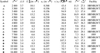
. For reference, the relevant boundary layer parameters of the experimental data are given in table 1. Throughout this paper the data from Sillero et al. (Reference Sillero, Jiménez and Moser2013) are presented either using (black) solid lines or symbols

 $\unicode[STIX]{x1D6FF}$
given by Chauhan et al. (Reference Chauhan, Monkewitz and Nagib2009) is consistently larger than
 $\unicode[STIX]{x1D6FF}_{99}$
, and an approximately constant fraction of the Rotta–Clauser length scale,
 $\unicode[STIX]{x1D6E5}$
, to within the uncertainty.
Details of the boundary layer database examined herein.

Here we present a brief description of the experimental data (with further details in Morrill-Winter et al.
Reference Morrill-Winter, Klewicki, Baidya and Marusic2015), which unlike the DNS data are more prone to errors from measurements and data processing. The experimental data were acquired in the Melbourne Wind Tunnel, formally referred to as the High Reynolds Number Boundary Layer Wind Tunnel (HRNBLWT) at University of Melbourne, and the Flow Physics Facility (FPF) at the University of New Hampshire, e.g. see Nickels et al. (Reference Nickels, Marusic, Hafez, Hutchins and Chong2007) and Vincenti et al. (Reference Vincenti, Klewicki, Morrill-Winter, White and Wosnik2013), respectively. Both facilities reach high Reynolds numbers by employing a long development fetch. This results in large viscous length scales, enabling well-resolved measurements using conventionally sized sensors. A custom multi-element hot-wire probe was used to acquire the data. This probe features four sensing elements; two wall parallel wires and a vertical cross-wire array. Altogether the sensor measures
 $\tilde{u}$
,
 $v$
,
 $uv$
and
 $\tilde{\unicode[STIX]{x1D714}}_{z}$
. Here
 $\tilde{\cdot }$
represents a total quality (mean plus fluctuation) and
 $\unicode[STIX]{x1D714}_{z}$
is the spanwise vorticity. The parallel wires are woven between the cross-wires centring the interrogation point for all statistics. Morrill-Winter et al. (Reference Morrill-Winter, Klewicki, Baidya and Marusic2015) implemented a unique calibration and processing scheme that solves for
 $v$
absent its mean value from the fluctuating voltages of the cross-wires, while determining
 $\tilde{u}$
from the single wires. This, for example, results in a greater level of consistency in the Reynolds stress profiles.
Estimating the terms in (1.1) from experimental data is challenging, as it contains derivatives of complicated quantities, such as the Reynolds stress and mean vorticity. Hence, for consistency, the viscous and the total stresses distributions (
 $\text{d}U^{+}/\text{d}y^{+}$
and
 $\text{d}U^{+}/\text{d}y^{+}+\langle -uv\rangle$
, respectively) are ‘smoothed’ as now described. Since close to the wall the distributions are invariant in viscous scaling, the highest Reynolds number DNS profile of Sillero et al. (Reference Sillero, Jiménez and Moser2013) (
 $\unicode[STIX]{x1D6FF}^{+}\simeq 2500$
), starting from
 $y^{+}=1$
to the first experimental point, is appended to the measured data. Note that the near wall measured data are expected to have larger measurement errors compared to data farther from the wall, since near the wall the velocity gradients are larger. Altogether, this gives a ‘stitched profile’ from the wall to the free stream. For completeness, the inner-normalized wall location of the first measurement point,
 $y_{min}^{+}$
is given in table 1. Subsequently, as shown in figure 1(a), a piecewise third-order polynomial (cubic-spline) is fitted in the least-square sense to the ‘stitched profile’, and forced to be contained between the boundary conditions (i.e. 1 at the wall and 0 in the free stream). A spline fit was selected to ensure no theoretical bias to the results, and because it provides an easily differentiable function. The same process was used to fit the total stress, which has the same boundary conditions as the viscous stress. Subtracting the functional form of the viscous stress from the total stress gives the spline fit of the Reynolds stress. Figure 1(a,b) provide an example and review of the smoothing process. Once the distribution for
 $\langle -uv\rangle$
has been obtained,
 $A$
can be evaluated from (1.1).
Illustration of the ‘smoothing’ procedure employed for the experimental data using
 $\unicode[STIX]{x1D6FF}^{+}\simeq 7000$
profile. (a) Viscous stress (
 $\text{d}U^{+}/\text{d}y^{+}$
) on a log–log plot, and (b) the total stress (
 $\text{d}U^{+}/\text{d}y^{+}+\langle -uv\rangle$
) on a linear–log plot for clarity. The

 $\unicode[STIX]{x1D6FF}^{+}\simeq 2400$
, and the grey lines (

 $y^{+}$
location of the peak in the Reynolds stress. The smoothing constant in the spline fit applied was
 $1{-}1.4\times 10^{-4}$
for all data sets.

Scaling of the MI term (
 $\overline{A}^{+}$
) from the experimental and DNS data. (a) The inner-normalized MI term against wall position normalized by inner (left panel) and outer (right panel) variables. The solid lines and the symbols

 $\unicode[STIX]{x1D6FC}$
parameter (
 $\overline{A}$
normalized by its peak value,
 $\overline{A}_{p}$
) versus outer-normalized wall position. (c) The peak in the MI term (
 $\overline{A}_{p}$
) versus Reynolds number,
 $\unicode[STIX]{x1D6FF}^{+}$
(left-hand side ordinate);
 $\overline{\unicode[STIX]{x1D6FC}}$
and
 $\text{}\underline{\unicode[STIX]{x1D6FC}}_{m}-\overline{\text{}\underline{\unicode[STIX]{x1D6FC}}_{m}}$
as a function of
 $\unicode[STIX]{x1D6FF}^{+}$
(right-hand side ordinate). The black fit lines in are
 $\overline{A}_{p}^{+}=1.76/\unicode[STIX]{x1D6FF}^{+}$
,
 $\overline{\unicode[STIX]{x1D6FC}}=0.57$
, and
 $\text{}\underline{\unicode[STIX]{x1D6FC}}_{m}=0.46$
. The grey lines in (c) are
 $\overline{A}_{p}^{+}=0.27/(\unicode[STIX]{x1D6FF}^{+})^{3/4}$
and
 $\overline{A}_{p}^{+}=11/(\unicode[STIX]{x1D6FF}^{+})^{5/4}$
, which are added to give perspective to the slope of
 $1/\unicode[STIX]{x1D6FF}^{+}$
. The intercepts were chosen such that all the fits lines would pass through the lowest
 $\unicode[STIX]{x1D6FF}^{+}$
point. Note, that a
 $\unicode[STIX]{x1D6FF}^{+}$
power deviating from
 $-1$
yields an intercept that is no longer
 $O(1)$
.

The inner-normalized terms present in (1.1) (thin (black) lines) and (3.5) (thick (blue) lines) at
 $\unicode[STIX]{x1D6FF}^{+}\simeq 2,400$
employing the DNS of Sillero et al. (Reference Sillero, Jiménez and Moser2013). The
 $VF^{+}$
is denoted by dashed lines (– – – -), whereas TI
 $^{+}$
and
 $\overline{A}^{+}$
is given by (——) and (– - – - –), respectively. The transformed Reynolds stress gradient (
 $\text{d}\tilde{T}/\text{d}y^{+}$
) and
 $\text{}\underline{\unicode[STIX]{x1D6FC}}_{m}(\unicode[STIX]{x1D6FF}^{+})/\unicode[STIX]{x1D6FF}^{+}$
in (3.5) are denoted by (– - – - – (blue)) and (—— (blue)), respectively. The grey line simply marks zero. The vertical dashed (red) lines are limits of the intermediate region provided by (4.4). Note that this is a continuous plot; however, we have employed different multipliers in different wall-normal regions so as to rescale the distributions for visual clarity.

3 Boundary layer mean equation transformation
For the purposes of elucidating Reynolds number invariant scaling behaviours, it is advantageous to manipulate (1.1) such that all leading-order terms are
 $O(1)$
and parameter free. The main aim of this section is to eliminate the
 $y$
dependence of the
 $\overline{A}$
term, and subsequently the TI term on the inertial domain. To this end, we employ high Reynolds number data to discern properties of the
 $\overline{A}$
and TI terms, and assess the veracity of the analytical treatments.
The procedure involves two steps. In § 3.1, the properties of the
 $\overline{A}$
-term in (1.1) are clarified. Here it turns out that an outer normalized form of the
 $\overline{A}$
distribution versus
 $y/\unicode[STIX]{x1D6FF}$
becomes invariant with increasing
 $\unicode[STIX]{x1D6FF}^{+}$
, which, incidentally, is also consistent with Townsend (Reference Townsend1976)’s outer layer similarity hypothesis. The analysis of § 3.2 involves transforming the TI and
 $\overline{A}$
terms so as to maintain their leading balance, but remove their individual dependencies on
 $y$
over the inertial domain.
3.1 Transformation of the
 $\overline{A}$
-term in (1.1)

Figure 2(a) illustrates properties of
 $\overline{A}^{+}(x^{+},y^{+})$
. With increasing scale separation (increasing
 $\unicode[STIX]{x1D6FF}^{+}$
), the peak in the
 $\overline{A}^{+}(x^{+})$
distribution,
 $\overline{A}_{p}^{+}(x^{+})$
, decreases yielding a flatter profile. Near the wall,
 $7\lesssim y^{+}\lesssim 40$
, the profile increases from zero to an amplitude that only increases slightly until the approximate location of the zero crossing of the TI term. (This region of slight increase appears to approach a plateau that diminishes in amplitude with increasing
 $\unicode[STIX]{x1D6FF}^{+}$
). The profile then increases to its peak, located at
 $y^{+}=O(\unicode[STIX]{x1D6FF}^{+})$
, or more precisely
 $y/\unicode[STIX]{x1D6FF}\simeq 0.57$
, and subsequently decreases to zero to satisfy the external boundary condition.
The desired transformation of
 $\overline{A}$
is found by first noting that
 $\overline{A}$
is zero at the inner and outer boundaries, and has a single peak. Thus, it may be represented as a fraction,
 $\unicode[STIX]{x1D6FC}(x,y)$
, of the peak magnitude,
 $\overline{A}_{p}(x)$
. This leads to
 $\overline{A}=\unicode[STIX]{x1D6FC}(x,y)\overline{A}_{p}(x)$
, where
 $0\leqslant \unicode[STIX]{x1D6FC}\leqslant 1$
. Note that the present
 $\unicode[STIX]{x1D6FC}$
differs from that used in Metzger et al. (Reference Metzger, Lyons and Fife2008). A compelling property of
 $\overline{A}_{p}^{+}(x^{+})$
is that when plotted versus
 $y/\unicode[STIX]{x1D6FF}$
, the location of its peak approximates constancy (figure 2
a).
Similarly, but more telling, figure 2(b) shows
 $\unicode[STIX]{x1D6FC}(x,y)$
plotted against outer-normalized wall location. All the data appear to merge except for those close to the wall. Under this scaling it is also apparent that
 $\unicode[STIX]{x1D6FF}$
(‘composite’) is appropriate boundary layer thickness as both the
 $\overline{A}$
and TI tend to zero at
 $y/\unicode[STIX]{x1D6FF}=1$
. The apparent invariance of
 $\unicode[STIX]{x1D6FC}(x,y)$
over
 $y/\unicode[STIX]{x1D6FF}$
suggests defining,
 $$\begin{eqnarray}\overline{\unicode[STIX]{x1D6FC}}:=\unicode[STIX]{x1D6FF}^{-1}\int _{0}^{\infty }\unicode[STIX]{x1D6FC}(x,y)\,\text{d}y,\end{eqnarray}$$
where, in practice, the upper limit of integration is the outermost measurement point (
 $y/\unicode[STIX]{x1D6FF}\approx 1.2$
), and suffices here because
 $\unicode[STIX]{x1D6FC}\rightarrow 0$
as
 $y\rightarrow \unicode[STIX]{x1D6FF}$
. Figure 2(c) shows
 $\overline{\unicode[STIX]{x1D6FC}}$
(with the ordinate on the right axis) for a range of Reynolds numbers. As is apparent,
 $\overline{\unicode[STIX]{x1D6FC}}$
exhibits constancy over the given
 $\unicode[STIX]{x1D6FF}^{+}$
range. The result that
 $\overline{\unicode[STIX]{x1D6FC}}$
is only a function of
 $\unicode[STIX]{x1D6FF}^{+}$
is non-trivial, and provides great simplification in further analytical development. This points to the fact that the mean advection is an outer scale phenomenon (similar to the wake contribution to the streamwise mean velocity profile), and consequently its ‘shape’ is self-similar and is invariant with
 $\unicode[STIX]{x1D6FF}^{+}$
in outer normalization (cf. figure 2
b). Now,
 $\overline{\unicode[STIX]{x1D6FC}}$
can be employed to normalize
 $\unicode[STIX]{x1D6FC}$
such that
 $\text{}\underline{\unicode[STIX]{x1D6FC}}(x,y):=\unicode[STIX]{x1D6FC}(x,y)/\overline{\unicode[STIX]{x1D6FC}}$
. Equation (1.1) then becomes:
 $$\begin{eqnarray}\frac{\text{d}^{2}U^{+}}{\text{d}y^{+2}}+\frac{\text{d}T^{+}}{\text{d}y^{+}}+\underbrace{\overline{\unicode[STIX]{x1D6FC}}(\unicode[STIX]{x1D6FF}^{+})\overline{A}_{p}^{+}(\unicode[STIX]{x1D6FF}^{+})}_{1/\unicode[STIX]{x1D6FF}^{+}}\text{}\underline{\unicode[STIX]{x1D6FC}}(x^{+},y^{+})=0.\end{eqnarray}$$
Even though we have presented both
 $\overline{\unicode[STIX]{x1D6FC}}$
and
 $\overline{A}_{p}^{+}$
as functions of
 $\unicode[STIX]{x1D6FF}^{+}(x^{+})$
or simply
 $x^{+}$
, inspection of all the experimental data presented in figure 2(c) shows a constant
 $\overline{\unicode[STIX]{x1D6FC}}=0.57\pm 0.047$
(one standard deviation). Also, figure 2(c) shows the decrease in
 $\overline{A}_{p}^{+}(x^{+})$
with increasing
 $\unicode[STIX]{x1D6FF}^{+}$
. In fact, the best fit power-law line has a
 $\unicode[STIX]{x1D6FF}^{+}$
exponent of
 $-1$
, indicating that both the peak magnitude and the location of
 $\overline{A}^{+}$
scale with
 $\unicode[STIX]{x1D6FF}^{+}$
. Fitting the data gives
 $\overline{A}_{p}^{+}=1.76/\unicode[STIX]{x1D6FF}^{+}$
. Therefore, on empirical grounds alone it is reasonable to replace
 $\overline{\unicode[STIX]{x1D6FC}}(\unicode[STIX]{x1D6FF}^{+})\overline{A}_{p}^{+}(\unicode[STIX]{x1D6FF}^{+})$
with
 $1.0032/\unicode[STIX]{x1D6FF}^{+}$
, or within experimental and rounding error, with
 $1/\unicode[STIX]{x1D6FF}^{+}$
.
In fact, however,
 $\overline{\unicode[STIX]{x1D6FC}}\overline{A}_{p}^{+}(\unicode[STIX]{x1D6FF}^{+})=1/\unicode[STIX]{x1D6FF}^{+}$
is an exact relation obtained by integrating (3.2) with respect to
 $y^{+}$
from
 $0$
to
 $\unicode[STIX]{x1D6FF}^{+}$
(or
 $\infty$
). Note that
 $\text{d}U^{+}/\text{d}y^{+}$
is equal to 1 and 0 at the wall and
 $y=\unicode[STIX]{x1D6FF}$
, respectively, whereas,
 $T^{+}$
vanishes at the boundaries. Furthermore, appendix A provides an explicit proof. This relation also provides a stringent check on the measurement accuracy. With this, (3.2) or the inner-normalized form of (1.1) can be written as,
 $$\begin{eqnarray}\frac{\text{d}^{2}U^{+}}{\text{d}y^{+2}}+\frac{\text{d}T^{+}}{\text{d}y^{+}}+\frac{1}{\unicode[STIX]{x1D6FF}^{+}}\text{}\underline{\unicode[STIX]{x1D6FC}}(y^{+},\unicode[STIX]{x1D6FF}^{+})=0.\end{eqnarray}$$
Note that here we have replaced the functional dependence on
 $x^{+}$
with
 $\unicode[STIX]{x1D6FF}^{+}$
. This indicates that the distribution of mean quantities is a function of
 $y^{+}$
and
 $\unicode[STIX]{x1D6FF}^{+}$
, which is indeed what is observed in experimental/DNS profiles after the initial or tripping effects are forgotten, leading to a nominally constant Coles’ wake factor.
We point out that, in the analysis of Klewicki (Reference Klewicki2013a
), the integral of the
 $\overline{A}$
is deduced to be
 $O(1)$
. Also, while the transformation of the mean advection term might seem relatively inconsequential since it resulted in
 $\text{}\underline{\unicode[STIX]{x1D6FC}}(y^{+},\unicode[STIX]{x1D6FF}^{+})=\unicode[STIX]{x1D6FF}^{+}\overline{A}^{+}$
, this transformation highlights an important scaling property of
 $\overline{A}$
. Namely, it is not at all apparent that
 $\unicode[STIX]{x1D6FF}^{+}\overline{A}^{+}$
is
 $O(1)$
when simply considering (1.1).
3.2 Transformation of the TI term in (1.1)
We have managed to represent the mean inertia (
 $\overline{A}$
) term of (1.1) in a form that explicitly contains the
 $1/\unicode[STIX]{x1D6FF}^{+}$
dependence found in the pipe and channel MMB; however, the properties of
 $\overline{A}$
, notably its peak (which follows outer scaling), is still present in
 $\text{}\underline{\unicode[STIX]{x1D6FC}}(y^{+},\unicode[STIX]{x1D6FF}^{+})$
. On the inertial domain
 $(1/\unicode[STIX]{x1D6FF}^{+})\text{}\underline{\unicode[STIX]{x1D6FC}}(y^{+},\unicode[STIX]{x1D6FF}^{+})$
balances the TI term in (3.2). It is, however, much easier to analyse the MMB if there is a balance between constant terms in the outer region (for any fixed
 $\unicode[STIX]{x1D6FF}^{+}$
). To this end, we now modify the TI term in a manner that transforms (3.3) such that the outer region balance is between (essentially)
 $y$
independent terms that only vary with
 $\unicode[STIX]{x1D6FF}^{+}$
.
The wall-normal position of the beginning of the inertial region is well represented by the location of the zero crossing of the TI term,
 $y_{m}$
, or equivalently the peak location of the Reynolds shear stress (e.g. Wei et al.
Reference Wei, Fife, Klewicki and McMurtry2005; Klewicki, Fife & Wei Reference Klewicki, Fife and Wei2009; Chin et al.
Reference Chin, Philip, Klewicki, Ooi and Marusic2014). To maintain this property for the modified TI term, we define the transformed Reynolds stress as,
 $$\begin{eqnarray}\tilde{T}:=T^{+}+\frac{1}{\unicode[STIX]{x1D6FF}^{+}}\int _{0}^{y^{+}}\unicode[STIX]{x1D6EC}(s,\unicode[STIX]{x1D6FF}^{+})\,\text{d}s,\end{eqnarray}$$
where,
 $\unicode[STIX]{x1D6EC}(y^{+},\unicode[STIX]{x1D6FF}^{+}):=\text{}\underline{\unicode[STIX]{x1D6FC}}(y^{+},\unicode[STIX]{x1D6FF}^{+})-\text{}\underline{\unicode[STIX]{x1D6FC}}_{m}(\unicode[STIX]{x1D6FF}^{+})$
, and
 $\text{}\underline{\unicode[STIX]{x1D6FC}}_{m}(\unicode[STIX]{x1D6FF}^{+}):=\text{}\underline{\unicode[STIX]{x1D6FC}}(y_{m},\unicode[STIX]{x1D6FF}^{+})$
. Using these definitions, equation (3.2) becomes
 $$\begin{eqnarray}\frac{\text{d}^{2}U^{+}}{\text{d}y^{+2}}+\frac{\text{d}\tilde{T}}{\text{d}y^{+}}+\frac{\text{}\underline{\unicode[STIX]{x1D6FC}}_{m}}{\unicode[STIX]{x1D6FF}^{+}}=0.\end{eqnarray}$$
Note that while
 $\text{}\underline{\unicode[STIX]{x1D6FC}}_{m}=\text{}\underline{\unicode[STIX]{x1D6FC}}_{m}(\unicode[STIX]{x1D6FF}^{+})$
is a possibility, the data of figure 2(b) indicate that
 $\text{}\underline{\unicode[STIX]{x1D6FC}}_{m}$
exhibits
 $\unicode[STIX]{x1D6FF}^{+}$
invariance, with
 $\text{}\underline{\unicode[STIX]{x1D6FC}}_{m}\simeq 0.46$
. This results in (3.5) being analogous to the inner-normalized MMB for channel/pipe flow. The construction of (3.5) preserves
 $\text{d}\tilde{T}/\text{d}y^{+}=0$
at
 $y=y_{m}$
. Figure 3 illustrates the repercussions of this transformation relative to the terms in (1.1), where the thick (blue) lines show the three terms in (3.5). For comparison the terms in (1.1) are presented in thin (black) lines. From the wall to the zero crossing in the Reynolds stress gradient the TI term remains essentially unchanged for both (1.1) and (3.5), with only an
 $O(1/\unicode[STIX]{x1D6FF}^{+})$
variation at the wall to account for
 $\text{}\underline{\unicode[STIX]{x1D6FC}}_{m}/\unicode[STIX]{x1D6FF}^{+}$
. Beyond
 $y_{m}$
, however, the reduced TI becomes to a constant negative value equal in magnitude to
 $\text{}\underline{\unicode[STIX]{x1D6FC}}_{m}/\unicode[STIX]{x1D6FF}^{+}$
. Note that the VF term remains unchanged everywhere.
4 Reduced mean dynamical scaling
To this point (1.1) has been recast as (3.5). This form closely corresponds to that of pipe and channel flows. The last term in (3.5) is analogous to the pressure gradient term in pipes or channels with an experimentally estimated Reynolds number independent constant,
 $\text{}\underline{\unicode[STIX]{x1D6FC}}_{m}$
, for boundary layers.
We are now in a position to carry out the analysis which involves identifying different regions in the boundary layer based on the leading balances of terms in (3.5), with analytical findings verified using experimental data. In § 4.2 we employ the rescaling transformations appropriate to the ‘intermediate region’ (which will be defined below). These analyses show that the location of peak Reynolds stress in turbulent boundary layers scales like
 $y_{m}^{+}\sim \sqrt{\unicode[STIX]{x1D6FF}^{+}}$
, which is corroborated by the present high
 $Re$
data.
4.1 Mean flow domains in boundary layers
The present analysis of (3.5) for boundary layers follows from the previous work of Fife et al. (Reference Fife, Klewicki, McMurtry and Wei2005a
) and Wei et al. (Reference Wei, Fife, Klewicki and McMurtry2005) for channels, and, as mentioned in § 1, considerably extends the previous boundary layer analysis of Klewicki (Reference Klewicki2013b
). Specifically, on the subdomains of primary interest the appropriate normalization not only aligns the actual order of magnitude of terms with the order of magnitude formally reflected by the given normalized form of the MMB, but expresses the subdominant term solely as a function of
 $\unicode[STIX]{x1D6FF}^{+}$
, i.e. as it appears in the pipe and channel flow MMB.
Under inner and outer normalizations the leading-order MMB is then reduced to two simpler forms that are respectively valid on a near-wall region and outer region. Namely, to leading-order VF
 $\simeq$
TI when
 $0\leqslant y\leqslant y_{in}$
, and TI
 $\simeq$
MI (
 $=\text{}\underline{\unicode[STIX]{x1D6FC}}_{m}/\unicode[STIX]{x1D6FF}^{+}$
) when
 $y_{out}\leqslant y\leqslant \unicode[STIX]{x1D6FF}$
, where
 $y_{in}$
and
 $y_{out}$
are the bounds of the domains where these balances hold. That is, the appropriate inner (
 $u_{\unicode[STIX]{x1D70F}}$
,
 $\unicode[STIX]{x1D708}/u_{\unicode[STIX]{x1D70F}}$
) and outer (
 $u_{\unicode[STIX]{x1D70F}}$
,
 $\unicode[STIX]{x1D6FF}$
) normalizations of (3.5) or (1.1) are valid over the domains
 $0\leqslant y\leqslant y_{in}$
, and
 $y_{out}\leqslant y\leqslant \unicode[STIX]{x1D6FF}$
, respectively. Estimates for
 $y_{in}$
and
 $y_{out}$
are empirically estimated herein over an unprecedented
 $\unicode[STIX]{x1D6FF}^{+}$
range (in § 4.3). Furthermore, in the domain,
 $y_{in}\leqslant y\leqslant y_{out}$
, all the terms in (3.5) are leading order. This is referred to as the intermediate region.
As in the classical theory,
 $u_{\unicode[STIX]{x1D70F}}$
is employed as the single appropriate velocity scale (e.g. Jones et al.
Reference Jones, Nickels and Marusic2008). This is consonant with the physical notion that a boundary layer converts free stream momentum flux into a surface shear force (e.g. Klewicki Reference Klewicki2010).
4.2 Intermediate scaling
The appropriate normalizations for
 $y$
and
 $\tilde{T}$
are not as obvious as for
 $U$
in the intermediate region. The following developments exploit the fact that
 $\text{d}T/\text{d}y=0$
at
 $y_{m}$
, and that
 $y_{in}<y_{m}<y_{out}$
. This must be true since at
 $y=y_{m}$
equations (3.5) or (1.1) reduces to a two term equation not containing the TI term. Like the inner and outer domains, the region bounding
 $y_{m}$
has location-specific scaling properties (Wei et al.
Reference Wei, Fife, Klewicki and McMurtry2005; Klewicki Reference Klewicki2013b
). Generically, these scaling properties will hold over a finite domain of size determined by the characteristic length scale of that domain. It is not a priori known whether this scaling domain extends over
 $y_{in}<y<y_{out}$
.
To determine the scaling properties and bounds of such a domain it is useful to fix one term in (1.1), and monitor how the other terms change relative to that constant. This was previously accomplished relative to (3.5) by transforming the
 $\overline{A}$
into a constant for any particular
 $\unicode[STIX]{x1D6FF}^{+}$
. Scaling properties are further clarified by transforming the modified MI term to unity, making it easier to compare the magnitude of this term with the two other terms in (3.5). To this end we follow Fife et al. (Reference Fife, Klewicki and Wei2009) and cast (3.5) into an invariant form by applying the differential transformations,
 $$\begin{eqnarray}\text{d}y^{+}=(\unicode[STIX]{x1D6FF}^{+}/\text{}\underline{\unicode[STIX]{x1D6FC}}_{m})^{1/2}\,\text{d}{\hat{y}},\quad \text{and}\quad \text{d}\tilde{T}=(\unicode[STIX]{x1D6FF}^{+}/\text{}\underline{\unicode[STIX]{x1D6FC}}_{m})^{-1/2}\,\text{d}\hat{T}.\end{eqnarray}$$
This results in
 $$\begin{eqnarray}\frac{\text{d}^{2}U^{+}}{\text{d}{\hat{y}}^{2}}+\frac{\text{d}\hat{T}}{\text{d}{\hat{y}}}+1=0.\end{eqnarray}$$
Equations (4.1) can be integrated with constants chosen such that
 ${\hat{y}}=0$
at
 $y^{+}=y_{m}^{+}$
(i.e. where
 $\text{d}\tilde{T}/\text{d}y^{+}=\text{d}T^{+}/\text{d}y^{+}=0$
) and
 $\hat{T}=0$
when
 $\tilde{T}=\tilde{T}|_{y_{m}}=\tilde{T}_{m}$
:
 $$\begin{eqnarray}\displaystyle y^{+}=(\unicode[STIX]{x1D6FF}^{+}/\text{}\underline{\unicode[STIX]{x1D6FC}}_{m})^{1/2}{\hat{y}}+y_{m}^{+},\quad \text{and}\quad \tilde{T}=(\unicode[STIX]{x1D6FF}^{+}/\text{}\underline{\unicode[STIX]{x1D6FC}}_{m})^{-1/2}\hat{T}+\tilde{T}_{m}. & & \displaystyle\end{eqnarray}$$
Equation (4.3a,b
) indicates that the peak location of the Reynolds stress is given by
 $y_{m}^{+}=C\sqrt{\unicode[STIX]{x1D6FF}^{+}}$
, where,
 $C$
is an
 $O(1)$
constant.
The monotonically decreasing behaviour of
 $\text{d}\tilde{T}/\text{d}y^{+}$
over an interior domain,
 $O(\unicode[STIX]{x1D708}/u_{\unicode[STIX]{x1D70F}})\leqslant y\leqslant O(\unicode[STIX]{x1D6FF})$
, is now exploited. From the wall,
 $\text{d}\tilde{T}/\text{d}y^{+}$
increases to a maximum inner peak that is much greater than
 $\text{}\underline{\unicode[STIX]{x1D6FC}}_{m}/\unicode[STIX]{x1D6FF}^{+}$
, and then decays to
 $-\text{}\underline{\unicode[STIX]{x1D6FC}}_{m}/\unicode[STIX]{x1D6FF}^{+}$
. Due to this behaviour, there exist wall-normal locations where
 $$\begin{eqnarray}\left[\frac{\,\text{d}\hat{T}}{\,\text{d}{\hat{y}}}=1=-2\frac{\text{d}^{2}U^{+}}{\,\text{d}{\hat{y}}^{2}}\right]_{{\hat{y}}={\hat{y}}_{mi}},\quad \text{and}\quad \left[\frac{\,\text{d}\hat{T}}{\,\text{d}{\hat{y}}}=-\frac{1}{2}=\frac{\text{d}^{2}U^{+}}{\,\text{d}{\hat{y}}^{2}}\right]_{{\hat{y}}={\hat{y}}_{mo}}.\end{eqnarray}$$
These locations approximately bound the domain of the intermediate region. Here we note that
 ${\hat{y}}_{mi}<{\hat{y}}_{m}<{\hat{y}}_{mo}$
, and although the scalings indicated in (4.3) might hold beyond
 ${\hat{y}}_{mi}$
and
 ${\hat{y}}_{mo}$
, they exactly satisfy (3.5) for
 ${\hat{y}}_{mi}$
,
 ${\hat{y}}_{m}$
, and
 ${\hat{y}}_{mo}$
. To understand the behaviour of
 ${\hat{y}}_{mi}$
and
 ${\hat{y}}_{mo}$
, with changing
 $\unicode[STIX]{x1D6FF}^{+}$
we have turn to observations. In the following we also show data pertaining to characteristics of the intermediate region.
Scaling in the intermediate regime. (a) The terms of (4.2) on along
 ${\hat{y}}$
for different
 $\unicode[STIX]{x1D6FF}^{+}$
. The (——) and

 $(\unicode[STIX]{x1D6FF}^{+}/\overline{\unicode[STIX]{x1D6FC}}_{m})^{1/2}$
. The solid black line is
 $y_{m}^{+}=1.47(\unicode[STIX]{x1D6FF}^{+}/\overline{\unicode[STIX]{x1D6FC}}_{m})^{1/2}$
. The grey lines are
 $y_{m}^{+}=10.5(\unicode[STIX]{x1D6FF}^{+}/\overline{\unicode[STIX]{x1D6FC}}_{m})^{1/4}$
and
 $y_{m}^{+}=0.21(\unicode[STIX]{x1D6FF}^{+}/\overline{\unicode[STIX]{x1D6FC}}_{m})^{3/4}$
, which are added to give perspective to the intermediate scaling. The intercepts were chosen such that all the fits would pass through the lowest
 $\unicode[STIX]{x1D6FF}^{+}$
point. (c) The nominal width (
 ${\hat{y}}_{mo}-{\hat{y}}_{mi}$
) and the beginning (
 ${\hat{y}}_{mi}$
) of the scaling domain. The dashed lines are best fit lines of the form
 ${\hat{s}}={\hat{s}}_{1}+({\hat{s}}_{0}-{\hat{s}}_{1})\text{e}^{\unicode[STIX]{x1D6FF}^{+}/\unicode[STIX]{x1D6E5}_{c}}$
. Where
 ${\hat{s}}$
is any hat variable,
 ${\hat{s}}_{0}$
and
 ${\hat{s}}_{1}$
are the starting and ending values of
 ${\hat{s}}$
, respectively, and
 $\unicode[STIX]{x1D6E5}_{c}$
is a constant.

4.3 Evidence from experiments and DNS
Figure 4(a) plots the terms in (4.2) using DNS and experimental data. They exhibit no apparent dependence on
 $\unicode[STIX]{x1D6FF}^{+}$
for increasing Reynolds number and over all
 ${\hat{y}}$
, except a low-
 $Re$
effect at smaller
 ${\hat{y}}$
, which will be discussed further below (in reference to figure 4
c). As such, the data agree with the rescaling analysis of the intermediate region. Figure 4(b) presents the wall-normal location of the Reynolds stress gradient zero crossing, showing that
 $y_{m}^{+}$
, follows a linear dependence when plotted versus
 $(\unicode[STIX]{x1D6FF}^{+}/\text{}\underline{\unicode[STIX]{x1D6FC}}_{m})^{1/2}$
. This is consistent with the invariance of (4.2). The slope of this line is approximately
 $1.47$
. With
 $\text{}\underline{\unicode[STIX]{x1D6FC}}_{m}\simeq 0.46$
, the location of the peak in
 $T^{+}$
is experimentally estimated by
 $y_{m}^{+}\simeq (1.47)(\unicode[STIX]{x1D6FF}^{+}/0.46)^{1/2}=2.17(\unicode[STIX]{x1D6FF}^{+})^{1/2}$
. These empirical estimates indicate that the location where the VF term loses leading order (i.e. where the mean dynamics become inertial) is
 $y^{+}=y_{m}^{+}+{\hat{y}}_{mo}(\unicode[STIX]{x1D6FF}^{+}/\text{}\underline{\unicode[STIX]{x1D6FC}}_{m})^{1/2}\simeq (1.47+1.0)(\unicode[STIX]{x1D6FF}^{+}/0.46)^{1/2}\simeq 3.6(\unicode[STIX]{x1D6FF}^{+})^{1/2}$
(with
 ${\hat{y}}_{mo}\simeq 1.0$
as shown in the next paragraph). Previous studies estimated the onset of the inertial domain to follow the same scaling, but with a leading coefficient closer to
 $2.6$
(Wei et al.
Reference Wei, Fife, Klewicki and McMurtry2005; Klewicki et al.
Reference Klewicki, Fife and Wei2009; Klewicki Reference Klewicki2013a
). Similarly, Marusic et al. (Reference Marusic, Monty, Hultmark and Smits2013) used
 $3(\unicode[STIX]{x1D6FF}^{+})^{1/2}$
to approximate the starting location for the inertial region in pipes and boundary layers, where the mean velocity and streamwise variance profiles exhibit logarithmic behaviour.
Figure 4(c) plots
 ${\hat{y}}_{mi}$
, and
 ${\hat{y}}_{mo}-{\hat{y}}_{mi}$
against
 $\unicode[STIX]{x1D6FF}^{+}$
. At most, these data exhibit only a very slight variation in
 ${\hat{y}}_{mi}$
for the given
 $\unicode[STIX]{x1D6FF}^{+}$
range, but display a more noticeable
 $\unicode[STIX]{x1D6FF}^{+}$
variation in the width of the domain (
 ${\hat{y}}_{mo}-{\hat{y}}_{mi}$
) – at least at low
 $\unicode[STIX]{x1D6FF}^{+}$
. These data suggest that the width of the domain approaches constancy with increasing
 $\unicode[STIX]{x1D6FF}^{+}$
. For
 $\unicode[STIX]{x1D6FF}^{+}\gtrsim 10\,000$
a plateau behaviour of
 ${\hat{y}}_{mi}$
and
 ${\hat{y}}_{mo}$
is observed in figure 4(c) , with
 ${\hat{y}}_{mi}\simeq -0.5$
and
 ${\hat{y}}_{mo}\simeq 1.0$
.
To proceed further, we note that the invariant form (4.2), which is of the same form as found for pipe and channel flows, should lead eventually to a log law for
 $U^{+}$
in the inertial region (Fife et al.
Reference Fife, Klewicki and Wei2009; Klewicki et al.
Reference Klewicki, Philip, Marusic, Chauhan and Morrill-Winter2014; Klewicki & Oberlack Reference Klewicki and Oberlack2015). To show this requires the construction of a hierarchy of scaling layers (patches), which is now addressed for the boundary layer. We should, however, mention that even though there are close similarities in the analysis with pipes/channels, they are not the same. The intermediate steps for which we shall provide experimental evidence depend on the boundary layer data, which of course differ from pipes and channels.
5 Continuous scaling layer hierarchy
As with the analysis of Fife et al. (Reference Fife, Klewicki, McMurtry and Wei2005a
) for channel flow, a continuum of scaling layer (patches) of increasing size are now found by satisfying the same criteria used to construct the intermediate layer described in § 4. This involves the use of a transformation that shifts the intermediate region along the wall-normal direction, so as to create a continuum of such intermediate patches. At present, even though it looks more like a mathematical construct, eventually it will indeed provide valuable information as in Fife et al. (Reference Fife, Wei, Klewicki and McMurtry2005b
), and more specifically to a log law. In essence, this is accomplished by adding and subtracting a small parameter,
 $\unicode[STIX]{x1D712}$
, to (3.5)
 $$\begin{eqnarray}\frac{\text{d}^{2}U^{+}}{\text{d}y^{+2}}+\frac{\text{d}\tilde{T}}{\text{d}y^{+}}-\unicode[STIX]{x1D712}+\frac{\text{}\underline{\unicode[STIX]{x1D6FC}}_{m}}{\unicode[STIX]{x1D6FF}^{+}}+\unicode[STIX]{x1D712}=0.\end{eqnarray}$$
This leads to
 $$\begin{eqnarray}\frac{\text{d}^{2}U^{+}}{\text{d}y^{+2}}+\frac{\text{d}T_{\unicode[STIX]{x1D712}}}{\text{d}y^{+}}+\frac{1}{W^{+2}}=0,\end{eqnarray}$$
where,
 $$\begin{eqnarray}T_{\unicode[STIX]{x1D712}}(y^{+};\unicode[STIX]{x1D712})\equiv \tilde{T}-\unicode[STIX]{x1D712}y^{+}=T^{+}+\frac{1}{\unicode[STIX]{x1D6FF}^{+}}\int _{0}^{y^{+}}\unicode[STIX]{x1D6EC}(s,\unicode[STIX]{x1D6FF}^{+})\,\text{d}s-\unicode[STIX]{x1D712}y^{+},\quad \text{and}\quad \frac{1}{W^{+2}}\equiv \frac{\text{}\underline{\unicode[STIX]{x1D6FC}}_{m}(\unicode[STIX]{x1D6FF}^{+})}{\unicode[STIX]{x1D6FF}^{+}}+\unicode[STIX]{x1D712},\end{eqnarray}$$
where,
 $W=W(\unicode[STIX]{x1D712})$
. Transformations (5.3) result in (5.2) attaining the same form as found for channel flow by Fife et al. (Reference Fife, Klewicki, McMurtry and Wei2005a
). In previous channel flow analyses, the small parameter was called
 $\unicode[STIX]{x1D6FD}$
. A different symbol,
 $\unicode[STIX]{x1D712}$
, is chosen here since the present construction for the boundary layer is slightly different. Like
 $\unicode[STIX]{x1D6FD}$
, however, the value of
 $\unicode[STIX]{x1D712}$
physically sets the wall-normal position where the three terms in (5.3) will balance each other. This position is associated with the zero crossing of
 $\text{d}T_{\unicode[STIX]{x1D712}}/\text{d}y^{+}$
. For decreasing
 $\unicode[STIX]{x1D712}$
, these positions move outward from the wall. This is shown in figure 5 for
 $\unicode[STIX]{x1D6FF}^{+}=2,400$
as an example, where we vary the parameter
 $\unicode[STIX]{x1D712}$
, and different lines represent a different
 $\unicode[STIX]{x1D712}$
value. Dictated by the definition, the zero crossing in
 $\text{d}T_{\unicode[STIX]{x1D712}}/\text{d}y^{+}$
moves wallward as
 $\unicode[STIX]{x1D712}$
increases. Figure 5(b) shows the corresponding effect on
 $T_{\unicode[STIX]{x1D712}}$
. It can be seen that when
 $\unicode[STIX]{x1D712}=0$
,
 $T_{\unicode[STIX]{x1D712}}=\tilde{T}$
and (3.5) is identical to (5.2), which is indicated by the dark (black) lines in the figure.
(a) Illustration of the modification to the transformed Reynolds stress gradient
 $\text{d}T_{\unicode[STIX]{x1D712}}/\text{d}y^{+}$
for varying
 $\unicode[STIX]{x1D712}$
. (b) Transformed Reynolds stress
 $T_{\unicode[STIX]{x1D712}}$
varying for changing parameter
 $\unicode[STIX]{x1D712}$
. The distribution is the DNS of
 $\unicode[STIX]{x1D6FF}^{+}\simeq 2400$
. The (——) denote
 $\unicode[STIX]{x1D712}=0$
. Changing colour red to green implies increasing
 $\unicode[STIX]{x1D712}$
, and the (

 $W$
scales do not hold, i.e. beyond the limits indicated by (5.4).

It is apparent that we cannot vary
 $\unicode[STIX]{x1D712}$
in an arbitrary fashion, if we still want to have the three terms in (5.2) to balance. As shown in the example in figure 5(a), increasing
 $\unicode[STIX]{x1D712}$
decreases the peak
 $\text{d}T_{\unicode[STIX]{x1D712}}/\text{d}y^{+}$
, and we cannot have any balance of the three terms if the peak of
 $\text{d}T_{\unicode[STIX]{x1D712}}/\text{d}y^{+}$
becomes negative, i.e.
 $(\text{d}T_{\unicode[STIX]{x1D712}}/\text{d}y^{+})_{peak}\geqslant 0$
, or,
 $\unicode[STIX]{x1D712}\leqslant (\text{d}\tilde{T}/\text{d}y^{+})_{peak}=(\text{d}T^{+}/\text{d}y^{+})_{peak}$
. On the other end, we want
 $\text{}\underline{\unicode[STIX]{x1D6FC}}_{m}/\unicode[STIX]{x1D6FF}^{+}+\unicode[STIX]{x1D712}\geqslant 0$
for the three-term balance. These two conditions results in the bounds for
 $\unicode[STIX]{x1D712}$
:
 $$\begin{eqnarray}-\frac{\text{}\underline{\unicode[STIX]{x1D6FC}}_{m}}{\unicode[STIX]{x1D6FF}^{+}}\leqslant \unicode[STIX]{x1D712}\leqslant \left(\frac{\text{d}T^{+}}{\text{d}y^{+}}\right)_{peak}.\end{eqnarray}$$
Now, we are in a position to make (5.2) invariant by following the same set of analytical steps as described for the intermediate layer above in § 4.2. This involves rescaling
 $\text{d}y^{+}$
and
 $\text{d}T_{\unicode[STIX]{x1D712}}$
as,
 $$\begin{eqnarray}\text{d}y^{+}=W^{+}\,\text{d}{\hat{y}},\quad \text{and}\quad \text{d}T_{\unicode[STIX]{x1D712}}=\frac{1}{W^{+}}\,\text{d}\hat{T}_{\unicode[STIX]{x1D712}},\end{eqnarray}$$
which when applied to (5.2) yields
 $$\begin{eqnarray}\frac{\text{d}^{2}U^{+}}{\text{d}{\hat{y}}^{2}}+\frac{\text{d}\hat{T}_{\unicode[STIX]{x1D712}}}{\text{d}{\hat{y}}}+1=0.\end{eqnarray}$$
Like (4.1), (5.5) can be integrated with integration constants chosen such that at
 ${\hat{y}}=0$
when
 $y^{+}=y_{m}^{+}(\unicode[STIX]{x1D712})$
, i.e. where
 $\text{d}T_{\unicode[STIX]{x1D712}}/\text{d}y^{+}=0$
, and
 $\hat{T}_{\unicode[STIX]{x1D712}}=0$
, when
 $T_{\unicode[STIX]{x1D712}}=T_{\unicode[STIX]{x1D712}}|_{y_{m}^{+}}=:T_{\unicode[STIX]{x1D712}m}(\unicode[STIX]{x1D712})$
. This leads to
 $$\begin{eqnarray}y^{+}=W^{+}{\hat{y}}+y_{m}^{+}(\unicode[STIX]{x1D712}),\quad \text{and}\quad T_{\unicode[STIX]{x1D712}}=\frac{1}{W^{+}}\hat{T}_{\unicode[STIX]{x1D712}}+T_{\unicode[STIX]{x1D712}m}(\unicode[STIX]{x1D712}).\end{eqnarray}$$
We note that
 $y_{m}^{+}$
and
 $\unicode[STIX]{x1D712}$
have one-to-one correspondence by construction, i.e. for every (continuous) value of the parameter
 $\unicode[STIX]{x1D712}$
, we have a corresponding
 $y_{m}^{+}$
, and vice versa. The above scaling is valid for every value of
 $\unicode[STIX]{x1D712}$
as long as
 $\unicode[STIX]{x1D712}$
is within the prescribed limits set by (5.4). From (5.5) it is clear that for a unit change in
 $\,\text{d}{\hat{y}}$
,
 $\text{d}y^{+}$
will change by
 $W^{+}$
, which of course is a function of
 $\unicode[STIX]{x1D712}$
. Consequently, we call
 $W^{+}$
the layer width, or the hierarchical layer width – hierarchical because of its continuous dependence on
 $\unicode[STIX]{x1D712}$
. The hat notation remained the same between the original intermediate layer analysis (in § 4.2) and the
 $W$
layer analysis. This is because the construction for each layer of width
 $W(\unicode[STIX]{x1D712})$
is simply a generalization of the same construction, which reduces to that presented in § 4.2 for
 $\unicode[STIX]{x1D712}=0$
. As before, we now define a region where the three terms in (5.6) are of the same order of magnitude.
 $$\begin{eqnarray}\left[\frac{\,\text{d}\hat{T}_{\unicode[STIX]{x1D712}}}{\,\text{d}{\hat{y}}}=1=-2\frac{\text{d}^{2}U^{+}}{\,\text{d}{\hat{y}}^{2}}\right]_{{\hat{y}}={\hat{y}}_{mi}(\unicode[STIX]{x1D712})},\quad \text{and}\quad \left[\frac{\,\text{d}\hat{T}_{\unicode[STIX]{x1D712}}}{\,\text{d}{\hat{y}}}=-\frac{1}{2}=\frac{\text{d}^{2}U^{+}}{\,\text{d}{\hat{y}}^{2}}\right]_{{\hat{y}}={\hat{y}}_{mo}(\unicode[STIX]{x1D712})}.\end{eqnarray}$$
Again,
 ${\hat{y}}_{mi}$
and
 ${\hat{y}}_{mo}$
can be taken as the approximate inner and outer location of the region where the three terms are
 $O(1)$
for a particular choice of
 $\unicode[STIX]{x1D712}$
. The definition of the limits in (5.8) and a monotonic change of terms in (5.6), ensures that,
 $$\begin{eqnarray}\unicode[STIX]{x0394}{\hat{y}}\equiv ({\hat{y}}_{mo}-{\hat{y}}_{mi})=O(1).\end{eqnarray}$$
The experimental evidence to be discussed in greater detail below in § 5.1 (cf. figure 7) clearly shows that
 $\unicode[STIX]{x0394}{\hat{y}}$
is not only
 $O(1)$
, but actually attains a value close to unity. In conjunction with (5.5) this implies that
 $$\begin{eqnarray}\unicode[STIX]{x0394}y^{+}(\unicode[STIX]{x1D712})=y_{mo}^{+}(\unicode[STIX]{x1D712})-y_{mi}^{+}(\unicode[STIX]{x1D712})=O(W^{+}(\unicode[STIX]{x1D712})).\end{eqnarray}$$
Equation (5.10) is one way to estimate the width of the hierarchical intermediate layer. There is, however, another more robust way. Recall that the location where
 $\text{d}T_{\unicode[STIX]{x1D712}}/\text{d}y^{+}=0$
is also where
 ${\hat{y}}=0$
, i.e.
 $y^{+}=y_{m}^{+}(\unicode[STIX]{x1D712})$
from (5.7), and lies between the inner and outer bounds of the intermediate region. At this location (5.6) indicates that
 $$\begin{eqnarray}\frac{1}{W^{+2}}=-\frac{\text{d}^{2}U^{+}}{\text{d}y^{+2}}\Bigg|_{y_{m}^{+}(\unicode[STIX]{x1D712})},\end{eqnarray}$$
which serves as a computationally more precise way of calculating
 $W^{+}$
.
There are two important properties for any layer, the width of the layer (
 $W^{+}(\unicode[STIX]{x1D712})$
) and the wall-normal location (say the ‘centre’) of the layer which we defined as the location of
 $\text{d}T_{\unicode[STIX]{x1D712}}/\text{d}y^{+}=0$
, i.e.
 $y^{+}=y_{m}^{+}(\unicode[STIX]{x1D712})$
. The width can be calculated from (5.11), whereas estimation of the location of the layer requires an analysis which follows Fife et al. (Reference Fife, Wei, Klewicki and McMurtry2005b
). We shall see that estimation of the location will lead us to the log law without any assumptions.
To this end, we estimate the order of magnitude
 $\text{d}^{3}U^{+}/\,\text{d}{\hat{y}}^{3}$
across any given
 $W$
layer separated by a distance
 $y_{mo}^{+}(\unicode[STIX]{x1D712})-y_{mi}^{+}(\unicode[STIX]{x1D712})$
. Consider a second-order central difference approximation about
 $y^{+}=y_{m}^{+}(\unicode[STIX]{x1D712})$
, i.e.
 ${\hat{y}}=0$
,
 $$\begin{eqnarray}\displaystyle \frac{\text{d}^{3}U^{+}}{\,\text{d}{\hat{y}}^{3}}\Bigg|_{y_{m}^{+}(\unicode[STIX]{x1D712})} & \simeq & \displaystyle \frac{\left.{\displaystyle \frac{\text{d}^{2}U^{+}}{\,\text{d}{\hat{y}}^{2}}}\right|_{{\hat{y}}_{mo}}-\left.{\displaystyle \frac{\text{d}^{2}U^{+}}{\,\text{d}{\hat{y}}^{2}}}\right|_{{\hat{y}}_{mi}}}{{\hat{y}}_{mo}-{\hat{y}}_{mi}}={\displaystyle \frac{-{\displaystyle \frac{1}{2}}-(-2)}{\unicode[STIX]{x0394}{\hat{y}}}}\nonumber\\ \displaystyle & & \displaystyle \unicode[STIX]{x0394}{\hat{y}}\simeq \frac{3}{2}\left(\frac{\text{d}^{3}U^{+}}{\,\text{d}{\hat{y}}^{3}}\Bigg|_{y_{m}^{+}(\unicode[STIX]{x1D712})}\right)^{-1}.\end{eqnarray}$$
The same can be obtained by applying the mean value theorem across the
 $W$
layer.
Since
 $\unicode[STIX]{x0394}{\hat{y}}=O(1)$
, we therefore surmise that
 $$\begin{eqnarray}\frac{\text{d}^{3}U^{+}}{\,\text{d}{\hat{y}}^{3}}\Bigg|_{y_{m}^{+}(\unicode[STIX]{x1D712})}=O(1).\end{eqnarray}$$
Now, differentiating (5.11) with respect to
 $\unicode[STIX]{x1D712}$
, and using the first equation in the transformation (5.5) results in
 $$\begin{eqnarray}\frac{-2}{W^{+3}}\frac{\text{d}W^{+}}{\text{d}\unicode[STIX]{x1D712}}=-\frac{\text{d}^{3}U^{+}}{\text{d}y^{+3}}\Bigg|_{y_{m}^{+}(\unicode[STIX]{x1D712})}\frac{\text{d}y_{m}^{+}}{\text{d}\unicode[STIX]{x1D712}},\quad \text{and}\quad 2\frac{\text{d}W^{+}}{\text{d}\unicode[STIX]{x1D712}}=\frac{\text{d}^{3}U^{+}}{\,\text{d}{\hat{y}}^{+3}}\Bigg|_{y_{m}^{+}(\unicode[STIX]{x1D712})}\frac{\text{d}y_{m}^{+}}{\text{d}\unicode[STIX]{x1D712}}.\end{eqnarray}$$
The last equation directly leads to
 $$\begin{eqnarray}2\left(\frac{\text{d}y_{m}^{+}}{\text{d}W^{+}}\right)^{-1}=\frac{\text{d}^{3}U^{+}}{\,\text{d}{\hat{y}}^{+3}}\Bigg|_{y_{m}^{+}(\unicode[STIX]{x1D712})}.\end{eqnarray}$$
Utilising (5.13) in (5.15) allows one to show that
 $\text{d}y_{m}^{+}/\text{d}W^{+}=O(1)$
, thus revealing that the wall-normal location of a particular
 $W$
layer scales with its width. That is, layers of larger width are located proportionally farther from the wall. Furthermore, since
 $y_{m}^{+}$
continuously varies across the
 $W$
layer hierarchy, a
 $y_{m}^{+}$
coincides with every
 $y^{+}$
, and therefore
 $$\begin{eqnarray}\unicode[STIX]{x1D719}(\unicode[STIX]{x1D712}):=\frac{\text{d}y^{+}}{\text{d}W^{+}}=O(1).\end{eqnarray}$$
Equation (5.16) holds within the limits of the layer hierarchy, which as mentioned before, is defined by the bounds on the parameter
 $\unicode[STIX]{x1D712}$
(cf. (5.4)). The parameter
 $\unicode[STIX]{x1D719}$
in (5.16) is called the Fife similarity parameter (e.g. see Klewicki et al.
Reference Klewicki, Philip, Marusic, Chauhan and Morrill-Winter2014; Klewicki & Oberlack Reference Klewicki and Oberlack2015). As shown in § 5.2, equation (5.16) leads to a log-law mean velocity profile. Before demonstrating that, experimental verifications of (5.16) and other results indicated above are provided.
The terms present in (5.6) at multiple values of
 $\unicode[STIX]{x1D712}$
at three different
 $\unicode[STIX]{x1D6FF}^{+}$
. (a)
 $\unicode[STIX]{x1D6FF}^{+}=2400$
, (b)
 $\unicode[STIX]{x1D6FF}^{+}=7000$
and (c)
 $\unicode[STIX]{x1D6FF}^{+}=16\,400$
. The DNS is given by (——) and


The inner and outer bounds of each layer on the hierarchy plotted versus
 $W^{+}$
. The DNS is given by


5.1 Evidence of hierarchical layer structure from experimental and DNS data
Figure 6(a–c) shows the terms in (5.6) for varying
 $\unicode[STIX]{x1D712}$
at three disparate
 $\unicode[STIX]{x1D6FF}^{+}=2400,7000$
and
 $16\,400$
, respectively. It is evident that with varying
 $\unicode[STIX]{x1D712}$
the various distributions merge about
 ${\hat{y}}=0$
, confirming the effectiveness of the transformations in (5.5).
Inner and outer bounds of each scaling layer normalized by wall units and plotted versus
 $y^{+}$
. The values are limited to
 $y^{+}<\unicode[STIX]{x1D6FF}^{+}/4$
due to the decreasing nature of the terms in (5.2).

The hierarchy layer widths
 $W^{+}$
against inner-normalized wall position for all
 $\unicode[STIX]{x1D6FF}^{+}$
presented herein. (a) Empirically determined from the data presented in figure 8. (b)
 $W^{+}$
evaluated directly from (5.11). The solid line (——) is the DNS of Sillero et al. (Reference Sillero, Jiménez and Moser2013) and the symbols are given in table 1. The grey line (

 $W^{+}=y^{+}/1.618$
given by Klewicki et al. (Reference Klewicki, Philip, Marusic, Chauhan and Morrill-Winter2014).

In (5.8) we defined the limits of the intermediate region of the
 $W$
layer hierarchy, and argued that this width
 $\unicode[STIX]{x0394}{\hat{y}}=O(1)$
(cf. equation (5.9)). This width is presented in figure 7 for different
 $\unicode[STIX]{x1D6FF}^{+}$
and varying
 $\unicode[STIX]{x1D712}$
. It is constructed by empirically locating the positions of
 ${\hat{y}}_{mi}$
and
 ${\hat{y}}_{mo}$
from figures like those presented in figure 6, and for each
 $\unicode[STIX]{x1D712}$
the width
 $W$
is evaluated from the second equation in (5.3). It is clear from the figure that, not only is
 $\unicode[STIX]{x0394}{\hat{y}}=O(1)$
, but rather it is numerically close to unity for all the
 $\unicode[STIX]{x1D6FF}^{+}$
and
 $\unicode[STIX]{x1D712}$
.
The data of
 ${\hat{y}}_{mi}$
and
 ${\hat{y}}_{mo}$
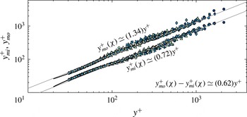
presented in figure 7 are shown in the more conventional wall units in figure 8, rather than in the
 $\hat{(.)}$
variables. For each
 $\unicode[STIX]{x1D6FF}^{+}$
, varying
 $\unicode[STIX]{x1D712}$
results in a unique
 $y_{m}^{+}(\unicode[STIX]{x1D712})$
(where
 $\text{d}T_{\unicode[STIX]{x1D712}}/\text{d}y^{+}=0$
), which is the abscissa. The ordinate is obtained from the first equation in (5.7), for example,
 $y_{mi}^{+}=W^{+}{\hat{y}}_{mi}+y_{m}^{+}(\unicode[STIX]{x1D712})$
. Given the range of
 $\unicode[STIX]{x1D6FF}^{+}$
and
 $\unicode[STIX]{x1D712}$
the linearity of
 $y_{mi}^{+}$
and
 $y_{mo}^{+}$
distributions is remarkable, but probably not surprising, given the fact that we already know that the width on the hierarchy scales linearly with the wall-normal distance (cf. (5.16)). This is discussed further below.
The most important result (towards a log law) is (5.16) which says that the width
 $W^{+}$
should scale linearly with
 $y^{+}$
. The width can be directly estimated from figure 8 as
 $W^{+}=y_{mo}^{+}-y_{mi}^{+}$
, and this is shown in figure 9(a). Rather than locating experimental points from graphs like figure 6 and then evaluating differences, it is more appropriate to employ (5.11) to evaluate
 $W^{+}$
, which is presented in figure 9(b). We recall that (5.11) is valid only at
 $y^{+}=y_{m}^{+}(\unicode[STIX]{x1D712})$
. Since, however, there is a one-to-one correspondence between
 $\unicode[STIX]{x1D712}$
and
 $y_{m}^{+}$
, a twice differentiation of the mean velocity profile can be used to compute
 $W^{+}$
. Estimation of
 $W^{+}$
by both methods shows that away from the boundaries, as discussed by Fife et al. (Reference Fife, Wei, Klewicki and McMurtry2005b
), we expect a linear behaviour of
 $W^{+}$
with respect to
 $y^{+}$
, which is amply clear from figure 9(a) and (b) in accordance with (5.16). A straight line
 $W^{+}=2y^{+}/(1+\sqrt{5})\simeq 0.618y^{+}$
is also shown in the figure; a value postulated by Klewicki et al. (Reference Klewicki, Philip, Marusic, Chauhan and Morrill-Winter2014) based upon the geometric structure of the layer hierarchy. Furthermore, and more directly from figure 8,
 $W^{+}=1.34y^{+}-0.72y^{+}=0.62y^{+}$
.
It follows from the above discussion that away from the boundaries, we should have
 $\unicode[STIX]{x1D719}=\text{d}y/\text{d}W=\text{const.}$
, say
 $\unicode[STIX]{x1D719}_{c}$
. In the inertial region which is indeed far away from the boundaries, with the inner location found above to be
 $y^{+}=3.6\sqrt{\unicode[STIX]{x1D6FF}^{+}}$
and an outer location fixed on a fraction of
 $\unicode[STIX]{x1D6FF}^{+}$
, we should expect
 $\unicode[STIX]{x1D719}=\unicode[STIX]{x1D719}_{c}=O(1)$
.
The present analysis and data show the basis for the often-used distance-from-the-wall scaling (Townsend Reference Townsend1976; Perry & Chong Reference Perry and Chong1982; Marusic & Kunkel Reference Marusic and Kunkel2003) argument employed in wall turbulence. We also mention that even though we concentrate only on the wall-normal distance, turbulent structures are three dimensional, and as such, the wall distance scaling has also been observed when considering the width of the structures in the spanwise direction too (e.g. Tomkins & Adrian Reference Tomkins and Adrian2003; Del Alamo et al. Reference Del Alamo, Jiménez, Zandonade and Moser2004).
5.2 Logarithmic mean velocity profile
With (5.6) and (5.16) one can follow the steps given in Klewicki & Oberlack (Reference Klewicki and Oberlack2015) to obtain the logarithmic mean profile via direct integration. As described by Fife et al. (Reference Fife, Klewicki and Wei2009), the self-similar structure described above holds on every layer of the hierarchy. As
 $y^{+}\rightarrow \infty$
, there is an interior domain on the hierarchy (the inertial sublayer) where the
 $W^{+}$
distribution approximates a linear function of
 $y^{+}$
, and with increasing
 $\unicode[STIX]{x1D6FF}^{+}$
this linearity becomes more exact. This stems from the fact that edge effects at the periphery of the overall layer hierarchy are the only influences that can disrupt similarity from layer to layer. Thus, as the number of hierarchy layers increases (
 $\unicode[STIX]{x1D6FF}^{+}\rightarrow \infty$
) the self-similar condition becomes increasingly exact over the interior inertial portion of the hierarchy, and accordingly,
 $\unicode[STIX]{x1D719}$
approaches constancy, i.e.
 $\unicode[STIX]{x1D719}\rightarrow \unicode[STIX]{x1D719}_{c}$
. The present boundary layer measurements support this in figure 9 by exhibiting nearly linear inertial layer
 $W^{+}(y^{+})$
profiles.
Substituting in the first equation of (5.14), i.e.
 $(2/W^{+3})(\text{d}y_{m}^{+}/\text{d}W^{+})^{-1}=(\text{d}^{3}U^{+}/\text{d}y^{+3})|_{y_{m}^{+}(\unicode[STIX]{x1D712})}$
, the expression for
 $W^{+}$
from (5.11), i.e.
 $W^{+}=(-\text{d}^{2}U^{+}/\text{d}y^{+2})^{-1/2}|_{y_{m}^{+}(\unicode[STIX]{x1D712})}$
, leads to,
 $$\begin{eqnarray}2\left(\frac{\text{d}y_{m}^{+}}{\text{d}W^{+}}\right)^{-1}=\frac{\text{d}^{3}U^{+}}{\text{d}y^{+3}}\Bigg|_{y_{m}^{+}(\unicode[STIX]{x1D712})}\left(-\frac{\text{d}^{2}U^{+}}{\text{d}y^{+2}}\right)^{-3/2}\Bigg|_{y_{m}^{+}(\unicode[STIX]{x1D712})}.\end{eqnarray}$$
As mentioned before,
 $y_{m}^{+}(\unicode[STIX]{x1D712})$
can be replaced by the variable
 $y^{+}$
on the layer hierarchy within the bounds of
 $\unicode[STIX]{x1D712}$
. Furthermore, adopting the definition of
 $\unicode[STIX]{x1D719}$
introduced in (5.16), setting
 $\unicode[STIX]{x1D719}=\unicode[STIX]{x1D719}_{c}$
and substituting this into (5.17) yields
 $$\begin{eqnarray}\frac{2}{\unicode[STIX]{x1D719}_{c}}=\frac{\text{d}^{3}U^{+}}{\text{d}y^{+3}}\left(-\frac{\text{d}^{2}U^{+}}{\text{d}y^{+2}}\right)^{-3/2}.\end{eqnarray}$$
With a value for
 $\unicode[STIX]{x1D719}_{c}$
specified, equation (5.18) constitutes a nonlinear differential equation with a single unknown,
 $U^{+}$
. Integration proceeds by letting
 $f=-\text{d}^{2}U^{+}/\text{d}y^{+2}$
, and then (5.18) becomes
 $$\begin{eqnarray}\frac{2}{\unicode[STIX]{x1D719}_{c}}f^{3/2}=-\frac{\text{d}f}{\text{d}y^{+}}.\end{eqnarray}$$
Separating variables and integrating yields
 $$\begin{eqnarray}f^{-1/2}=\frac{1}{\unicode[STIX]{x1D719}_{c}}(y^{+}+C),\end{eqnarray}$$
and squaring and inverting this result gives
 $$\begin{eqnarray}f\equiv -\frac{\text{d}^{2}U^{+}}{\text{d}y^{+2}}=\unicode[STIX]{x1D719}_{c}^{2}(y^{+}+C)^{-2}.\end{eqnarray}$$
Two more integrations yield
 $$\begin{eqnarray}U^{+}=\unicode[STIX]{x1D719}_{c}^{2}\text{ln}(y^{+}+C)+C_{1}y^{+}+C_{2},\end{eqnarray}$$
where
 $C_{1}$
and
 $C_{2}$
are integration constants.
The least-squares fit of
 $\unicode[STIX]{x1D719}_{c}$
and
 $C_{1}$
for
 $y_{i}\leqslant y^{+}\leqslant 0.2\unicode[STIX]{x1D6FF}$
against
 $\unicode[STIX]{x1D6FF}^{+}$
. The DNS of Sillero et al. (Reference Sillero, Jiménez and Moser2013) is given by

 $s=s_{1}+(s_{0}-s_{1})\text{e}^{\unicode[STIX]{x1D6FF}^{+}/\unicode[STIX]{x1D6E5}_{c}}$
. Here
 $s$
is either
 $\unicode[STIX]{x1D719}_{c}$
or
 $C_{1}$
,
 $s_{0}$
and
 $s_{1}$
are the starting and ending values of
 $s$
, respectively, and
 $\unicode[STIX]{x1D6E5}_{c}$
is a constant. The black lines correspond to
 $\unicode[STIX]{x1D719}_{c}=1.618$
from Klewicki et al. (Reference Klewicki, Philip, Marusic, Chauhan and Morrill-Winter2014), and
 $C_{1}=0$
.

Relative to the most familiar form of the log law
 $\unicode[STIX]{x1D719}_{c}^{2}$
is given by
 $\unicode[STIX]{x1D705}^{-1}$
(
 $\unicode[STIX]{x1D705}=$
von Kármán constant),
 $C_{1}=0$
, and
 $C$
is a small offset (
 $-7\lesssim C\lesssim 7$
) that is typically omitted owing to its negligible contribution to the profile behaviour on inertial domain. Klewicki & Oberlack (Reference Klewicki and Oberlack2015) explored the behaviours of
 $\unicode[STIX]{x1D719}$
and
 $C_{1}$
with increasing
 $\unicode[STIX]{x1D6FF}^{+}$
for channel flow using DNS data up to
 $\unicode[STIX]{x1D6FF}^{+}\simeq 5000$
. Consistent with the present theory, these data evidenced that
 $\unicode[STIX]{x1D719}\rightarrow \unicode[STIX]{x1D719}_{c}\simeq 1.6$
, and
 $C_{1}\rightarrow 0$
. The domain over which the log law will be considered here (inertial subdomain) is
 $3.6\sqrt{\unicode[STIX]{x1D6FF}^{+}}\leqslant y^{+}\leqslant 0.2\unicode[STIX]{x1D6FF}^{+}$
. The offset
 $C$
is challenging to determine when
 $\unicode[STIX]{x1D6FF}^{+}$
becomes large due to the starting point in the inertial region moving away from the wall in viscous units, e.g. see discussion in Klewicki (Reference Klewicki2013b
). Therefore, it was only determined for the DNS using (5.21) over the inertial subdomain. It was found be
 $0<C\lesssim 7$
with no clear
 $\unicode[STIX]{x1D6FF}^{+}$
trend where
 $C\simeq 3.2$
for the highest DNS profile. As a conservative estimate, if one considers
 $C=7$
, the difference in the start of the inertial domain between including the offset and neglecting it is
 $7.4\,\%$
and
 $1.7\,\%$
for
 $\unicode[STIX]{x1D6FF}^{+}\simeq 1000$
and
 $\unicode[STIX]{x1D6FF}^{+}\simeq 10\,000$
, respectively.
The values of
 $\unicode[STIX]{x1D719}_{c}$
and
 $C_{1}$
are estimated using the DNS and experimental data by least squares fitting the once-integrated form of (5.21) (the viscous stress) and neglecting
 $C$
. The results of this analysis are given in figure 10. With increasing
 $\unicode[STIX]{x1D6FF}^{+}$
both coefficients appear to approach constant values. Specifically
 $C_{1}\rightarrow 0$
. Here the data scatter precludes a discussion of the exact values of
 $\unicode[STIX]{x1D719}_{c}$
and
 $C_{1}$
. The results suggest, however, that both approach constants at a similar
 $\unicode[STIX]{x1D6FF}^{+}$
(
 ${\sim}10\,000$
), and that
 $C_{1}\rightarrow 0$
faster than
 $1/\unicode[STIX]{x1D6FF}^{+}\rightarrow 0$
. This latter point is significant since, while it is known that
 $C_{1}\rightarrow 0$
as
 $\unicode[STIX]{x1D6FF}^{+}\rightarrow \infty$
since
 $\text{d}U^{+}/\text{d}y^{+}\rightarrow 0$
as
 $y^{+}\rightarrow \infty$
, for
 $C_{1}$
to be negligible on the inertial domain at finite Reynolds numbers it must approach zero faster than
 $1/\unicode[STIX]{x1D6FF}^{+}$
.
6 Summary and conclusions
In the MMB equation for turbulent pipes and channels, the viscous and the (turbulent) inertia terms balance the pressure gradient term
 $1/\unicode[STIX]{x1D6FF}^{+}$
. As we move away from the wall the viscous terms diminishes, and the dominant balance is between two constant inertial terms (
 ${\sim}1/\unicode[STIX]{x1D6FF}^{+}$
). The constancy of these two terms considerably simplifies the analysis of the MMB. This simplification leads to many important characteristics of wall turbulence in pipes and channels, such as, an unambiguous layer structure depending on the balance of the three terms in the MMB, an analytically well-founded prediction for a logarithmic region in the mean velocity profile, along with the result that the beginning of the logarithmic region moves away from the wall like
 $C_{1}\sqrt{\unicode[STIX]{x1D6FF}^{+}}$
.
For the flat plate turbulent boundary layer previous MMB based analyses could not specify as much. The reason being that, even though the form of the viscous and turbulent inertia terms in the MMB for a zero pressure gradient turbulent boundary layer (ZPG-TBL) are the same as that for pipes and channels, the constant pressure gradient term is replaced by the advection term
 $-(U^{+}\unicode[STIX]{x2202}U^{+}/\unicode[STIX]{x2202}x^{+}+V^{+}\unicode[STIX]{x2202}U^{+}/\unicode[STIX]{x2202}y^{+})$
which varies with wall distance. This led some to question even the logarithmic form of
 $U^{+}$
in the ZPG-TBL, but with no such controversy for pipes/channels (e.g. George Reference George2007). To date, the primary attempts to resolve this issue have employed empirical data (e.g. Marusic et al.
Reference Marusic, Monty, Hultmark and Smits2013). This ambiguity, however, is not likely to be resolved by data alone, owing to the many practical measurement limitations, and the need for asymptotically large Reynolds numbers.
Analyses herein manipulate the MMB for the ZPG-TBL and show that the mean inertia term can be replaced by
 $\text{}\underline{\unicode[STIX]{x1D6FC}}_{m}/\unicode[STIX]{x1D6FF}^{+}$
, as accompanied by commensurate modifications to the turbulent inertia term. A constant value of
 $\text{}\underline{\unicode[STIX]{x1D6FC}}_{m}\sim 0.46$
was obtained using well-resolved boundary layer data that extend up to large
 $\unicode[STIX]{x1D6FF}^{+}$
, supplemented with existing DNS data. The physical reasoning for this transformation is that the mean inertia term (like the
 $1/\unicode[STIX]{x1D6FF}^{+}$
term in pipes/channels) adheres to an inertial layer scaling. Thus, even though the mean inertia changes with wall distance, the ‘shape’ is invariant with Reynolds number (or
 $\unicode[STIX]{x1D6FF}^{+}$
), and the ‘magnitude’ of the term is simply a function of
 $\unicode[STIX]{x1D6FF}^{+}$
and varies exactly as
 $1/\unicode[STIX]{x1D6FF}^{+}$
, as in the pipes/channel. The empirical observations underpinning the theoretical manipulations were only possible because of the range of the present high resolution data.
These findings led us to show that the beginning of the inertial region is located at an approximate
 $y^{+}$
-position of
 $3.6\sqrt{\unicode[STIX]{x1D6FF}^{+}}$
(where,
 $\unicode[STIX]{x1D6FF}$
is the based on the ‘composite’ velocity profile of Chauhan et al., Reference Chauhan, Monkewitz and Nagib2009), and that the peak location of
 $\langle -uv\rangle ^{+}$
varies as
 $y_{m}^{+}=2.17\sqrt{\unicode[STIX]{x1D6FF}^{+}}$
, confirmed by the high
 $Re$
experimental data.
The constancy in the mean inertia term is then employed to form a hierarchy of intermediate scaling layers in manner similar to Fife et al. (Reference Fife, Wei, Klewicki and McMurtry2005b
) (however, with differences peculiar to boundary layer and a change of logical emphasis). We show that the width of these layers (
 $W^{+}$
) scale linearly with distance from the wall, i.e.
 $\unicode[STIX]{x1D719}:=\text{d}y/\text{d}W=O(1)$
. These and further intermediate results are shown to be readily verifiable by high resolution Reynolds number data spanning over a decade, which among other results show that
 $\unicode[STIX]{x1D719}$
is a constant,
 $\unicode[STIX]{x1D719}_{c}$
, away from the boundaries with experimentally determined value of
 $\unicode[STIX]{x1D719}_{c}\approx 1.6$
. The linear scaling of the widths, or the constancy of
 $\unicode[STIX]{x1D719}$
leads to a theoretical derivation of the log law, with the von Kármán constant,
 $\unicode[STIX]{x1D705}=1/\unicode[STIX]{x1D719}_{c}^{2}$
.
Existing observations indicate that, to within measurement uncertainty, the logarithmic slope of pipe and boundary layer mean velocity profiles become indistinguishable at sufficiently high Reynolds numbers (e.g. Marusic et al. Reference Marusic, Monty, Hultmark and Smits2013; Furuichi et al. Reference Furuichi, Terao, Wada and Tsuji2015). The present analytical developments describe a scenario for how the appropriately transformed MMB for the boundary layer approaches the same mathematically self-similar structure as found for pipe and channel flows. High resolution measurements over an unprecedented Reynolds number range support the indicated scenario. Stemming from the apparently insurmountable indeterminacy caused by time averaging the Navier–Stokes equations, solutions to the MMB are not, however, mathematically unique. That said, features seemingly unique to the structure predicted by the present theory (such as the properties of the scaling layer hierarchy demonstrated herein) do indeed appear to reflect the physically realized structure of the flow in considerable detail.
Acknowledgements
This work was supported by the Australian Research Council and the US National Science Foundation.
Appendix A. Proof that
$\overline{\unicode[STIX]{x1D6FC}}(\unicode[STIX]{x1D6FF}^{+})\overline{A}_{p}^{+}(\unicode[STIX]{x1D6FF}^{+})=1/\unicode[STIX]{x1D6FF}^{+}$

This identity comes from integrating (3.2) from
 $y^{+}=0$
to
 $\infty$
:
 $$\begin{eqnarray}\int _{0}^{\infty }\frac{\text{d}^{2}U^{+}}{\text{d}y^{+2}}\text{d}y^{+}+\int _{0}^{\infty }\frac{\text{d}T^{+}}{\text{d}y^{+}}\text{d}y^{+}+\int _{0}^{\infty }\left(\overline{\unicode[STIX]{x1D6FC}}(\unicode[STIX]{x1D6FF}^{+})\overline{A}_{p}^{+}(\unicode[STIX]{x1D6FF}^{+})\text{}\underline{\unicode[STIX]{x1D6FC}}(x^{+},y^{+})\right)\,\text{d}y^{+}=0.\end{eqnarray}$$
Note that
 $\text{d}U^{+}/\text{d}y^{+}$
is equal to 1 and 0 at the wall and
 $y^{+}=\unicode[STIX]{x1D6FF}^{+}$
, respectively, whereas,
 $T^{+}$
vanishes at the boundaries.
 $$\begin{eqnarray}\displaystyle -1+\overline{\unicode[STIX]{x1D6FC}}(\unicode[STIX]{x1D6FF}^{+})\overline{A}_{p}^{+}(\unicode[STIX]{x1D6FF}^{+})\int _{0}^{\infty }\text{}\underline{\unicode[STIX]{x1D6FC}}(x^{+},y^{+})\,\text{d}y^{+}=0. & & \displaystyle\end{eqnarray}$$
Now, rewriting (3.1) shows that,
 $$\begin{eqnarray}\unicode[STIX]{x1D6FF}^{+}=\frac{1}{\overline{\unicode[STIX]{x1D6FC}}}\int _{0}^{\infty }\unicode[STIX]{x1D6FC}(x^{+},y^{+})\,\text{d}y^{+}=\int _{0}^{\infty }\frac{\unicode[STIX]{x1D6FC}(x^{+},y^{+})}{\overline{\unicode[STIX]{x1D6FC}}}\,\text{d}y^{+}=\int _{0}^{\infty }\text{}\underline{\unicode[STIX]{x1D6FC}}(x^{+},y^{+})\,\text{d}y^{+}.\end{eqnarray}$$
Substituting (A 3) into (A 2) yields,
 $$\begin{eqnarray}\overline{\unicode[STIX]{x1D6FC}}(\unicode[STIX]{x1D6FF}^{+})\overline{A}_{p}^{+}(\unicode[STIX]{x1D6FF}^{+})=(\unicode[STIX]{x1D6FF}^{+})^{-1}.\end{eqnarray}$$