Through the beginning of the twentieth century, Europeans dominated migrant flows to the United States, arriving freely with few laws restricting entry. This era of free mass migration ended abruptly in the 1920s with the Immigration Acts of 1921 and 1924 which imposed quotas to curtail European migration to the United States; however, migration from Mexico remained relatively unrestricted.Footnote 1 More individuals from Mexico arrived in the United States during the 1920s than did migrants from many European countries (see Figure 1). Mexican migrants became an increasingly important source of labor in the United States in the early twentieth century, yet little is known about those who decided to migrate and, among the migrants, those who decided to either stay or return.
Immigrant Flows to the United States, 1900–1929

In this paper we measure the pattern of selection into migration, and then examine whether there is any differential selection into return migration. Because only some individuals are willing to cross borders and leave their native land, the economic consequences of the quality of migrants relative to those who remain behind could affect the home and host economies through multiple channels (Borjas Reference Borjas1987). For the United States, the specific pattern of selection affects both migrant assimilation (Chiswick Reference Chiswick1978; Borjas Reference Borjas1985; Ferrie Reference Ferrie1999) and the return to migration (Abramitzky et al. Reference Abramitzky, Boustan and Eriksson2012). For Mexico, whether those leaving were of higher or lower quality than those staying is important for understanding potential “brain drain” (Gibson and McKenzie Reference Gibson and McKenzie2011), as well as income inequality (McKenzie and Rapoport Reference McKenzie and Rapoport2007).
If migrants were better than the general Mexican population in terms of productivity, education, or health, then they were positively self-selected.Footnote 2 To determine the pattern of selection one can compare the wages that Mexican migrants would earn in Mexico to the wages of those in Mexico who do not migrate (Borjas Reference Borjas1987). However, migrants and their wages are typically only observed in the host country. As prices for skills vary from country to country, comparing wages once migrants have crossed the border does not give the proper counterfactual. Techniques used to circumvent this problem and generate the appropriate comparison of migrants and non-migrants include propensity score matching (Chiquiar and Hanson Reference Chiquiar and Hanson2005) and sibling fixed effects (Abramitzky et al. Reference Abramitzky, Boustan and Eriksson2012).
Further, in many cases individual wages are not known. Some studies of historical selection use aggregated measures of human capital, such as occupational scores, to compare movers to stayers (Abramitzky et al. Reference Abramitzky, Boustan and Eriksson2012; Collins and Wanamaker Reference Collins and Wanamaker2014). However, if occupations reported in the historical immigration statistics were not representative of an individual's place in the skill distribution because migrants listed downgraded occupations on arrival that reflected labor demand in the United States, then these data would systematically underestimate the true quality of a migrant worker. Additionally, occupational scores are not specific to the individual and do not allow us to look at how migrants differed from the home population within reported occupation or skill class.
We use height as an alternative measure of the historical self-selection of Mexican migrants. A long literature argues that greater stature is correlated with higher earnings, greater intelligence, and increased health; in other words, height is positively correlated with “quality” (Steckel Reference Steckel1995; Steckel Reference Steckel2009). A migrant's height does not change as he crosses the border into the United States, unlike occupation or wages. Further, height gives a partial measure of human capital that is specific to the individual, important when there is little variation in migrant occupation. Since the vast majority of Mexican migrants claimed laborer or miner as their occupation, we are able to determine if the United States received the better laborers or the better miners by using height data.
Much of the migration from Mexico to the United States was temporary, and many individuals returned home instead of settling permanently (Gratton and Merchant Reference Gratton and Merchant2013). Measuring the selection into migration is not sufficient for understanding the effect of migrants on the labor force in both Mexico and the United States since return migrants might be differentially self-selected (Borjas and Bratsberg Reference Borjas and Bratsberg1996). However, the direction of selection for return migrants is unclear. Return migrants may have been “target earners” who migrated to accumulate savings in order to start a business back home, making the direction of selection ambiguous (Mesnard Reference Mesnard2004; Piore Reference Piore1979). On the other hand, return migrants could have been those who unexpectedly failed in the United States labor market and would thus be negatively self-selected (Abramitzky et al. Reference Abramitzky, Boustan and Eriksson2014). Further, pressure on Mexicans to leave the country or deportation drives that began to occur in the late 1920s and 1930s could have changed the quality of return migrants (Hoffman Reference Hoffman1974).
We utilize newly collected data from individual border manifests for migrants crossing through border towns in Arizona and Texas in 1920. To determine the selection of the migrant population compared to the home population, we compare heights for migrants to samples of heights for soldiers in the military and for those who applied for passports in Mexico.Footnote 3 Having estimated the self-selection of inflows, we estimate the self-selection of outflows. To do this, we link our sample of migrants who crossed the border in 1920 to the 1930 United States Census to create a sample of permanent migrants, and to the 1930 Mexican Census to create a sample of return migrants. We compare the heights of each sample to determine the self-selection of return migrants relative to permanent migrants.
We find that Mexican migrants in 1920 were positively self-selected on height from the Mexican population. They were four to five centimeters taller than soldiers in the military—typically members of the lower class of Mexican society—and they were only one and a half centimeters shorter than passport holders—typically members of the higher class of Mexican society (López-Alonso and Condey 2003). Our result holds within occupational skill class as the United States received the taller laborers, the taller skilled workers, and the taller professionals. We also find that although a substantial proportion of Mexican migrants returned home (between 13 and 44 percent), there was no differential self-selection on height into return migration. Our measured result of positive selection for migrant inflows is a good proxy for the change in the quality of the overall stock of Mexican migrants in the United States in the early twentieth century.
U.S.—MEXICO MIGRATION IN 1920
There is an extensive literature on the history of migration between the United States and Mexico (see Lawrence Cardoso (Reference Cardoso1980), Patrick Ettinger (Reference Ettinger2009), and David Gutierrez (Reference Gutiérrez1995) for an overview). Indeed, Mexican migration patterns transformed dramatically during the early twentieth century. The Mexican Revolution pushed migrants out during the 1910s, while the immigration quotas of 1921 and 1924 curtailed unskilled labor from Eastern and Southern Europe in the 1920s and pulled Mexican workers into the United States. We choose 1920 as a benchmark year, falling as it does directly between these two major events, to reveal how the self-selection process operated with limited, confounding institutional factors.
While there were some restrictions to entering the country in 1920, picking a year prior leads to several challenges for our analysis. First, most of the fighting in the Mexican Revolution occurred between 1910 and 1917, making it difficult to separate migrants moving for economic reasons versus those fleeing as refugees. Although some small amount of fighting continued in 1920, it was limited to the North while most of our sample comes from central Mexico. Second, the United States only started to systematically collect immigrant records for individuals crossing the Mexican border in 1907, and the process was not firmly in place by 1909, the year before the Mexican Revolution (Immigration Act of 1907, Sec. 32).
The Mexican Revolution, a multi-sided conflict, raged during the early 1910s although the major fighting subsided by 1917.Footnote 4 At the beginning of the Revolution, conflict occurred throughout Mexico as revolutionaries from different states fought to overthrow President Díaz, with the most intense fighting occurring between 1913 and 1916. Following the creation of a new constitution in 1917, major warfare subsided with only Pancho Villa skirmishing in small battles in the North. By 1920 most fighting halted as Villa surrendered and Álvaro Obregón was elected to the presidency (Knight Reference Knight1986).
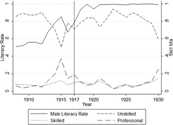
During the Revolution, thousands of Mexicans temporarily fled to the United States (United States Bureau of Immigration 1914). As refugees fled during the Revolution, migrant flows became more skilled between 1913 and 1916, the most intense period of fighting. By the end of the 1910s, however, the skill mix of the inflow had returned to pre-Revolutionary levels (see Figure 2). Even though thousands crossed the border, the United States absorbed these migrants easily as World War I increased the demand for labor (Rockoff Reference Rockoff2004). In fact, in 1917 the United States encouraged temporary Mexican migrants to work in agriculture, railroads, and mining, briefly suspending entry restrictions by allowing contract laborers, discontinuing the head tax, and waiving the literacy requirement (Cardenas Reference Cardenas1975). By 1920 thousands of Mexicans traveled northward yearly to earn higher wages offered by employers in the United States, but many of these same migrants later returned home (Clark Reference Clark1908; United States Bureau of Immigration 1920). In fact, Paul Taylor (Reference Taylor1929), in his extensive study of Mexican migrants, notes that many employers in the 1920s perceived Mexicans to be more reliable than other workers and attempted to keep them from returning home after the harvest season.
Skill Composition and Literacy Rate of Mexican Migrants, 1908–1930

As Congress was encouraging migration to the United States from Mexico, they simultaneously passed qualitative restrictions on migration in 1917 by requiring migrants to be able to read and write in their own language, potentially limiting illiterate Mexican individuals. However, the United States did not consistently enforce this law for Mexican migrants, first waiving the literacy requirement in 1917 and reissuing the waiver time to time until 1921 (Cardenas Reference Cardenas1975; Cardoso Reference Cardoso1976). The waiving of the literacy test is clear when comparing male migrant literacy rates to the skill mix of inflows, as we show in Figure 2. Prior to the literacy test in 1917, literacy and migrant skill level were positively correlated, as expected. Following 1917, however, the migrant flow became less skilled but more literate. By 1920 the percent unskilled was even higher than just before 1917, while the literacy rate increased to 99.4 percent. Even when agricultural workers were waived from the literacy test and head tax, official statistics probably still recorded them as literate.
The literacy test did not appear to restrict migration from Southern and Eastern Europe substantially. Congress imposed quantitative restrictions in 1921 and 1924, dramatically reducing migration from Europe (Zeidel Reference Zeidel2004). The quota system, however, placed no limits on migrants coming from the Western Hemisphere, and so Mexican migration was relatively unimpeded. Following the quotas, Mexican immigration increased dramatically as Mexicans acquired jobs due to a labor shortfall (Bloch Reference Bloch1929). The large increase in numbers would eventually lead to concerns over the racial origins of Mexican migrants (Foerster Reference Foerster1925), to the creation of the Mexican Border Patrol, and to the criminalization of undocumented entry in the 1920s (Ngai Reference Ngai2002).
SELECTION INTO MIGRATION
Migrants are not a random draw from their home country's population. Borjas (Reference Borjas1987) argued that we can predict the direction of self-selection for migrants based on the relative distribution of wages across economies. He finds that if the United States has a more unequal income distribution than the sending country, then we can expect positive selection into migration to the United States. If the migrants who leave from the home country are on average better (for example, more motivated, more educated, more productive, and so on) than those who stay, then the self-selection is positive; if migrants are worse along these dimensions than stayers, then self-selection is negative.
Selection is influenced by the variation in expected benefits of migration across the human capital distribution of potential migrants. In the early twentieth century, the benefits of migration were immediate as job opportunities were plentiful for Mexican workers. In the southwestern United States, many farms, railroads, and mines hired migrants directly at the border (United States Bureau of Immigration 1920). Mexicans typically worked in these sectors in the Southwest, but throughout the 1920s meatpackers and manufacturers in the Midwest and Northeast would recruit Mexicans from cities in Texas to replace jobs typically given to Southern and Eastern Europeans (Taylor Reference Taylor1929). While low-skilled jobs were readily available, high-skilled jobs were not as prevalent. Also, wages were higher for these unskilled laborers than in Mexico, suggesting a significant return to migration for unskilled laborers, which could lead to negative self-selection (Clark Reference Clark1908).
Selection is also influenced by the variation in costs of migration across the human capital distribution of potential migrants. While high wages abroad may entice a low-skilled individual to move, his mobility might be restricted by the costs of moving (for example, transportation, psychological, informational, or opportunity costs). Chiquiar and Hanson (2005) extend the Borjas (Reference Borjas1987) model by adding costs to reconcile the theoretical prediction that contemporary Mexican migrants should be negatively self-selected with the empirical evidence that they are intermediately self-selected. This shift in the literature from focusing on the benefits of migration to the costs of migration has been used to explain differential patterns of Mexican migrant selection from urban and rural areas and from places with different intensities of migrant networks (Fernández-Huertas Moraga Reference Moraga2011; McKenzie and Rapoport Reference McKenzie2010).
The benefits to migration were clear but high costs may have constrained individuals from traveling. While improvements in transportation from central Mexico to the United States border, especially the completion of the Mexican railroad in the late nineteenth century, lowered the cost of migration and subsequently spurred large waves of emigration, the cost of a ticket from central Mexico to the United States border was still high for poorer individuals (Clark Reference Clark1908; Coatsworth Reference Coatsworth1981). Additionally, the 1917 migration legislation required all migrants to pay an eight dollar head tax. Although the enforcement of this law during 1920 is unclear, if low-earning individuals were unable to finance the trip abroad, then self-selection could have been positive.
While a handful of papers analyze the selection of migrants from Europe (Abramitzky et al. Reference Abramitzky, Boustan and Eriksson2012, Reference Abramitzky, Boustan and Eriksson2014; Hatton and Williamson Reference Hatton, Williamson, Foders and Langhammer2006; Stolz and Baten Reference Stolz and Baten2012), little is known about selection of Mexican migration to the United States during the early twentieth century. Zadia Feliciano (Reference Feliciano2001) is the only paper to our knowledge that explores the historical self-selection of Mexican migrants, finding that in 1910 Mexicans in the United States had a higher rate of literacy than did the general Mexican population. We extend her results by incorporating evidence on immigrants following the Mexican Revolution, by using a measure (height) that is constant across borders, and by exploring the self-selection of return migrants which could alter the quality of the stock of Mexican migrants observed in the census.
HEIGHT AS A MEASURE OF SELECTION
Multiple metrics of human capital have been used in studies of selection, including income (Chiquiar and Hanson Reference Chiquiar and Hanson2005), skill class (Hatton and Williamson Reference Hatton, Williamson, Foders and Langhammer2006), occupational scores (Abramitzky et al. Reference Abramitzky, Boustan and Eriksson2014; Collins and Wanamaker Reference Collins and Wanamaker2014), age-heaping (Stolz and Baten Reference Stolz and Baten2012; A'Hearn et al. Reference A'Hearn, Baten and Crayen2009), and years of education and literacy (Feliciano Reference Feliciano2001). We have no data on the wages and education level of Mexican migrants in 1920, and so we use height to measure the quality of an individual migrant.
When income and wage data are not available, economists must rely on other measures to proxy for standard of living. In particular, height as a measure has been used since it is positively correlated with income and improved health and nutrition.Footnote 5 Higher living standards with ample food during childhood increase height, while poor nutrition and health can stunt growth.
Not only does the average height of a society indicate overall health and well-being, but taller people also earn more than their shorter counterparts within a country. For example, Paul Schultz (Reference Schultz2002) shows that a one centimeter increase in height leads to an 8 to 10 percent increase in wages in Brazil and Ghana. The return to physical strength is especially important in developing countries where large sectors of the economy rely on the physical productivity of labor. Height is a determinant of wages in these countries since larger and stronger men (as measured by Body Mass Index) are rewarded in the labor market (Thomas and Strauss Reference Thomas and Strauss1997). Mexican migrants worked in labor-intensive industries, such as mining, railroad construction, and farm labor, where improved physiology could lead to higher productivity (Clark Reference Clark1908; United States Bureau of Immigration 1920).
Nicola Persico, Andrew Postlewaite, and Dan Silverman (Reference Persico2004) argue that higher wages for taller individuals are due to non-cognitive characteristics (for example, confidence), while others (Case and Paxson Reference Case and Paxson2008; Schick and Steckel Reference Schick and Steckel2010) argue that early childhood inputs into health and nutrition can increase the cognitive functioning of an individual later in life. For example, taller individuals are more likely to remember their exact date of birth (Humphries and Leunig Reference Humphries and Leunig2009) and taller individuals score higher on early childhood cognitive and non-cognitive tests (Case and Paxson Reference Case and Paxson2008). Either way, the evidence suggests that taller individuals, on average, earn higher wages. If the migrants who arrived in the United States were taller than those who remained in Mexico, then this would indicate a pattern of positive selection for Mexican migrants.
DATA
Border Crossing Manifests
To understand exactly who migrated to the United States from Mexico in 1920, we construct a unique dataset from the manifest lists for those crossing at the border towns of Ajo, Arizona; Douglas, Arizona; Brownsville, Texas; and El Paso, Texas in 1920.Footnote 6 In Figure 3 we show the geographical coverage of our sample.Footnote 7 Height was recorded on each manifest by border officials and was often rounded to the nearest quarter inch. In addition to height, much more information about migrants upon arrival was recorded on the manifest, including demographic (age, sex, marital status), geographic (place of birth, place of last residence, intended destination), economic (occupation, savings), and network (join a friend, relative, or employer) data. We collect all available data for each adult male (18 years or older) classified as an immigrant.Footnote 8 In total, we have microdata for 3,671 male migrants who crossed the border in 1920.
To determine the representativeness of our sample, we compare the characteristics of our migrants with those of similar migrants recorded in the 1920 United States Census. We use the 1 percent 1920 Integrated Public Use Microdata Series (IPUMS) sample to identify migrants who arrived in the previous year, who were literate, over the age of 18, and male (Ruggles et al. Reference Ruggles2010). Our sample is representative of the distribution of skills for migrants recorded in the census with no statistical difference in occupational mix.Footnote 9 There is also no difference in marital status, although our sample is about two years younger and overrepresented by people moving to Texas.Footnote 10
Location of Border Stations and Regions in Mexico

Our dataset captures only documented migrants.Footnote 11 Although Louis Bloch (Reference Bloch1929), in a comparison of census numbers with net migration flows, estimates that undocumented entries could have been substantial for the decade from 1910 to 1920, he also admits that there is a lack of reliable information to make a study of this population feasible. To be precise, our results apply to those migrants who crossed through official border crossing stations, and not necessarily to all migrants.
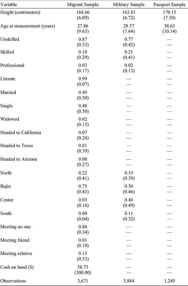
The border-crossing data allow us to create a profile for the “typical,” documented, male migrant who crossed the border from Mexico to the United States in 1920, as shown in Table 1. Male migrants to the United States were, on average, 29 years old, equally likely to be married as single, and almost universally recorded as literate. In Figure 3 we show the regional classification we use for the state of birth.Footnote 12 Immigrants came most often from central and northern Mexico, with very few coming from the southern states.Footnote 13 A large portion of our migrants were born in the Mexican states of Chihuahua, Guanajuato, and Jalisco, which are still high-sending states today, and most reported a final destination of Texas. Only 14 percent of migrants in the sample reported meeting someone (friend, relative, or employer) upon entry, much lower than Europeans in 1920 with 83 percent of Germans, 96 percent of Italians, and 97 percent of Greeks joining a network upon arrival.Footnote 14 On average, Mexican migrants brought $39 across the border.
We classify migrants as unskilled, skilled, or professional workers based on their reported occupation.Footnote 15 The majority (about 87 percent) of immigrants in the sample were unskilled. It is because of this lack of variation in skill class that occupational rankings yield little information in determining self-selection. Height allows us to examine whether migrants, within a given occupational class, were better or worse than non-migrants remaining in Mexico.
Summary Statistics for Migrant, Military, and Passport Samples

Notes:
Standard deviations are in parentheses. Proportions are reported unless otherwise noted.
Source:
Border crossing manifests and López-Alonso (Reference López-Alonso2003).
Comparison Samples: Military and Passport Data
To make an inference about the selection of migrants from Mexico we need to compare the heights of migrants to those living within Mexico. Here we use two distinct samples—military soldiers and passport holders. Howard Bodenhorn, Timothy Guinnane, and Thomas Mroz (Reference Bodenhorn, Guinnane and Mroz2013) warn that samples of historical heights are likely selected, which could lead to incorrect inferences about the underlying population. We acknowledge that both of these samples are not representative as the military sample is from the lower part of the height distribution of Mexico and passport records are from the upper part of the height distribution of Mexico (López-Alonso Reference López-Alonso2007, Reference Abramitzky, Boustan and Eriksson2012; López-Alonso and Condey Reference López-Alonso2003). However, by comparing migrants to both samples and determining which sample migrants most closely resemble we can infer whether migrants were positively or negatively selected.
The Secretaría Nacional de la Defensa houses federal military records in the Archivo de Concentración, recording deceased soldiers in the Sección de Personal Extinto and deserters in the Sección de Cancelados (López-Alonso and Condey Reference López-Alonso2003).Footnote 16 Since the military did not have required service until 1939, only those who made the choice to join the military appear in the data.
Characteristics of the military sample are also listed in Table 1. We show that 77 percent of military males were in unskilled occupations and that individuals were well represented across different regions of Mexico. At first glance, the military sample appears to be higher skilled than the migrant group, since 87 percent of migrants were unskilled compared to 77 percent of individuals in the military, implying negative self-selection. However, migrants may have reported intended occupation rather than previous occupation, leaving their true position in the skill distribution of Mexico unclear. Importantly, a comparison of average height reveals that migrants were nearly five centimeters taller than those in the military. We illustrate this comparison in Figure 4 by showing that the estimated height distribution for the migrant sample lies well to the right of the estimated height distribution for the military sample.
Heights: Immigrants, Soldiers, and Passport Applicants
We also compare migrants to a sample of passport applications from Mexico collected by López-Alonso (Reference López-Alonso2003) from the Archivo de Pasaportes. Unfortunately, this sample only includes age and does not give region of birth or skill classifications. Height was not measured for passports but was self-reported, possibly creating an upward bias since height tends to be over-reported (Spencer et al. Reference Spencer2002). Summary statistics in Table 1 show that passport applicants were only about one and a half centimeters taller than those immigrating to the United States. In Figure 4 we show that the estimated height distribution for the migrant sample lies very close to the estimated height distribution for the passport sample. While the average migrant was nearly five centimeters taller than the average member of the military, he was similar in height to the average passport applicant.
ESTIMATING SELF-SELECTION INTO MIGRATION
We utilize a linear regression model to explore the pattern of selection among Mexican migrants in 1920 as measured by migrant height. Although the analysis of the estimated densities in Figure 4 suggests a pattern of positive selection, it is possible that greater stature is simply correlated with other characteristics that are more prevalent in the migrant sample, such as a particular region of birth. Thus, we estimate Equation (1) to control for many of these additional characteristics that could confound our positive selection result.

An individual's height is regressed on a constant, an indicator variable for whether or not the individual is from the migrant sample, and a vector of controls. Final adult height may not be reached until 24 years of age and so individuals who are between 18 and 24 years might still be growing. We include dummy variables for age bins of 18–20 years and 21–23 years in order to account for this pattern.Footnote 17 We also include controls for decade of birth to account for any conditions that may have affected the height of all those born in Mexico during those times.Footnote 18 Furthermore, we include geographic controls to account for any spatial pattern in Mexican heights.Footnote 19 Finally, we include variables for occupational skill class which allows us to describe how migrants differed from others within skill class.
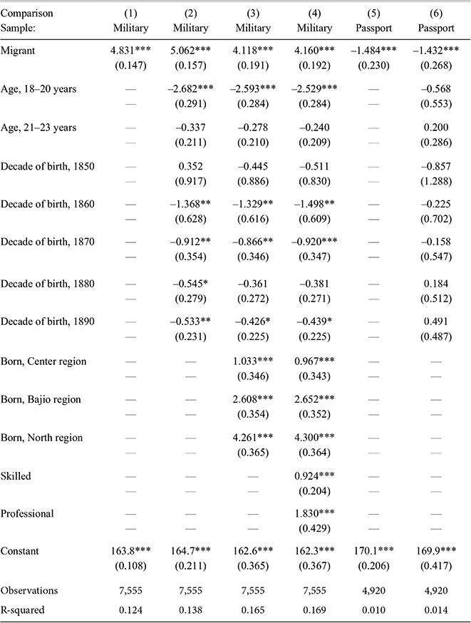
Results of the selection regressions comparing the sample of male migrants to the sample of males in the Mexican military are presented in Table 2, Columns (1)–(4). First, our estimates reveal expected patterns in heights. For example, adults in the 18–20 year age bin were shorter than adults over 24 years old, while those in the 21–23 year age bin were only slightly shorter and the difference loses statistical significance, consistent with human growth patterns. Also, those in the skilled class were taller than those in the unskilled class, while those in the professional class were taller than individuals in either of the other two occupational skill classes, supporting the claim that height is correlated with income, productivity, and cognitive ability. Second, the result of positive selection as measured by height holds in each of these specifications, with the migrant sample measuring four to five centimeters taller than those individuals in the military sample. Migrants were taller than those in the military even though they reported lower-skilled occupations. Finally, in Column (4) we show that migrants were taller than those in the military within occupational skill class. Although the descriptive statistics show that those who chose to migrate tended to come from lower-skilled occupations, we find that within skill class the individuals who migrated tended to be taller than those who were in the military.
1920 Selection Regressions Comparing Migrants to the Military and Passport Samples

* = Significant at the 10 percent level.
** = Significant at the 5 percent level.
*** = Significant at the 1 percent level.
Notes:
Robust standard errors are in parentheses. The omitted categories are those over age 24, those born prior to 1850, those born in the South region, and unskilled workers.
Source:
Border crossing manifests and López-Alonso (Reference López-Alonso2003).
We also present in Table 2 the results of selection regressions comparing the sample of male migrants to the sample of males applying for Mexican passports in Columns (5) and (6). Column (5) again shows a simple comparison of means between migrants and passport applicants, while Column (6) includes controls for ages less than 24 years and decade of birth. Those in the migrant sample were, on average, just under a centimeter and a half shorter than those in the passport sample. Given that the difference in height is quite small and the fact that those holding passports probably came from the upper end of the distribution in Mexican society, this is additional evidence consistent with a pattern of positive selection into Mexican migration in 1920.
Robustness Checks
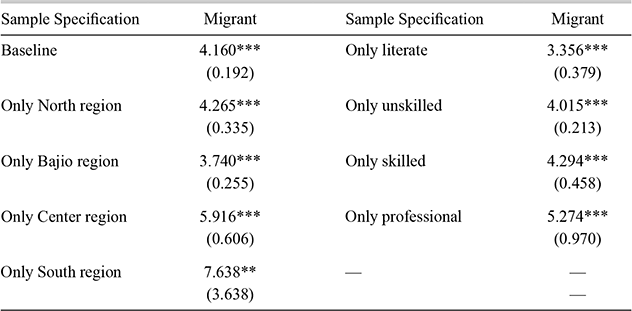
We present alternative specifications in Table 3 to address concerns about the Mexican Revolution and the effect of the 1917 literacy test requirement. It is possible that the self-selection result is not due to economic forces but rather because of refugees fleeing the Mexican Revolution. We test for differences in the pattern of selection by region of birth to determine whether positive selection was strongest in the North where fighting continued, and show the results in Table 3. Similar to the result found for the whole sample in the main specification, migrants born in the northern parts of Mexico were just over four centimeters taller than non-migrants and did not exhibit an abnormal or extraordinary pattern of selection that would give cause for concern.
It is possible that the pattern of positive selection resulted from the literacy test imposed in 1917, which could have barred low-quality Mexican migrants. While the degree of enforcement of the literacy test for Mexican migrants in 1920 is ambiguous as discussed earlier, we compare our sample of migrants to a subsample of 3,884 military deserters for whom we have literacy data, recognizing that there is a difference in how literacy is determined in the migrant and military samples. The literacy test required the migrant to read and write a paragraph of 25 words in a language of his choosing (Goldin Reference Goldin, Goldin and Libecap1994), while literacy in the military sample was determined by whether the soldier could sign his name (López-Alonso and Condey Reference López-Alonso2003). Our finding that migrants were positively selected still holds when comparing literate samples, and literate migrants were more than three centimeters taller than their counterparts in the military.
Alternative Sample Specifications for Migrant Selection Regressions

* = Significant at the 10 percent level.
** = Significant at the 5 percent level.
*** = Significant at the 1 percent level.
Notes:
Robust standard errors are in parentheses. The dependent variable in each regression is height. Each regression includes the full set of controls for age, location of birth, and occupation, but only the coefficient on migrant is reported. The comparison group is the military sample.
Source:
Border crossing manifests and López-Alonso (Reference López-Alonso2003).
Our results indicate that documented migrants to the United States in 1920 were positively self-selected from the home distribution but do not account for undocumented entry. Bloch (Reference Bloch1929) estimates that roughly 111,000 undocumented individuals entered the United States over the decade ending in 1920.Footnote 20 Using this number in combination with the official statistics for migration in the 1910s, a back of the envelope calculation suggests that the average undocumented migrant would need to have been 154.29 centimeters tall (9.5 centimeters shorter than the average male in the military and 14.5 centimeter shorter than the average documented migrant) to erase the height advantage over the military.Footnote 21 This means that even though institutional constraints could cause negatively self-selected individuals to migrate unofficially, it is unlikely that undocumented migration would cause a reversal of our positive selection result.
ACCOUNTING FOR RETURN MIGRATION
Selection into Return Migration
Measuring just the selection into migration is not sufficient to understand its long-term impact, especially when return migration was prevalent as in the case of Mexico. Even though migrants were positively self-selected from the Mexican population, return migrants could be differentially selected from the overall set of migrants, changing the quality of the stock of migrants that remained in the United States permanently and the quality of the stock of labor in Mexico (Borjas Reference Borjas1985; Borjas and Bratsberg Reference Borjas and Bratsberg1996).
Whether migrants who made the decision to return were positively or negatively self-selected from the migrant population is ambiguous. One possibility is that most migrants were “target earners” and returned when enough was saved to invest in capital back home, leaving their quality relative to permanent migrants unclear (Mesnard Reference Mesnard2004; Angelucci Reference Angelucci2012). Alternatively, if return migrants were those who failed in the labor market (Abramitzky et al. Reference Abramitzky, Boustan and Eriksson2014), then return migrants would have been negatively self-selected.
Another possibility is that return migrants did not make the decision on their own and were not voluntarily “self”-selected, but were forcibly removed by federal officials as the labor market tightened at the onset of the Great Depression. Historians have placed emphasis on the injustices surrounding mass deportations of Mexicans, with some estimating that more than one million Mexicans, including children and U.S. citizens, left the United States either forcibly or under the threat of removal (Balderrama and Rodriguez Reference Balderrama and Rodriguez2006). There is a debate, however, over the size of the dramatic fall in the Mexican population during the 1930s and whether the decrease was due to deportation or voluntary departure (Gratton and Merchant Reference Gratton and Merchant2013; Taylor Reference Taylor1934). Much of the mass departure could simply have been a result of the worsening economic conditions.
Most of this massive outflow of Mexicans occurred later during the 1930s, outside the years of this study, but there was a significant southward movement in the late 1920s. Some of this outward flow was due to official deportations under warrants, which increased almost 400 percent from 1,751 in 1925 to 8,438 in 1930 (Reports of the Commissioner General of Immigration 1925, 1930). This number of deportations in 1930 was larger than the 6,296 Mexicans leaving voluntarily, according to U.S. statistics. Mexican statistics, which are more reliable than U.S. data, suggest that deportations may not have been as important. According to Mexican sources, 70,129 individuals returned during 1930, making official deportations a much smaller percentage of total repatriations (Hoffman Reference Hoffman1974; Taylor Reference Taylor1929).Footnote 22 However, many more Mexicans may have left under the threat of deportation rather than being legally deported. Although the importance of deportations is under debate, the selection of return migrants on height could be altered by deportation pressures, depending on who was pressured to leave or forcibly removed.
Linked Sample
To estimate the selection of return migrants, we link our sample of 3,671 migrants forward to the 1930 United States Census for a sample of permanent migrants, and forward to the 1930 Mexican Census to get a sample of return migrants. The link to the 1930 United States Census is based on four characteristics: first name, last name, year of birth, and country of birth (Mexico). We also link our sample to the 1930 Mexican Census based on the same four characteristics, but are able to match on state of birth in Mexico. We follow an iterative matching procedure similar to Abramitzky, Boustan, and Eriksson (Reference Abramitzky, Boustan and Eriksson2014).Footnote 23 In order to limit bias from transcription errors, we also standardize names using the Double Metaphone algorithm.Footnote 24
Our linking strategy produces a set of migrants who are uniquely linked to the United States Census or to the Mexican Census, linked to multiple people in the same census, not linked to either census, or linked to both censuses. Failure to link to either census is most likely due to death, name change, or transcription error, while linking to both censuses or multiple times to the same census is likely due to extremely common names. These groups are dropped from the sample. From the original 3,671 migrants, we have a sample of 632 individuals uniquely linked to the 1930 Mexican Census and 798 uniquely linked to the 1930 United States Census.Footnote 25
There are 632 return migrants out of a total 1,430 uniquely linked migrants, which yields a 44.2 percent return rate after ten years of stay. This rate is likely an upper bound for the true rate of return since transcription error and name changes were more likely to occur in the United States. It is likely that transcription errors were more prevalent in the United States than in Mexico as Mexican enumerators were more familiar with Spanish names. Further, name changes were more likely to occur in the United States as some migrants anglicized their names to gain favor in the labor market (Biavaschi et al. Reference Biavaschi, Giulietti and Siddique2013). By comparison, the return migration rate for males calculated with administrative data for the decade from 1920 to 1930 is approximately 13.3 percent.Footnote 26 However, these administrative records probably undercounted out-migrants and therefore provide a lower bound on out-migration rates (Bandiera et al. Reference Bandiera, Rasul and Viarengo2013; Taylor Reference Taylor1929).
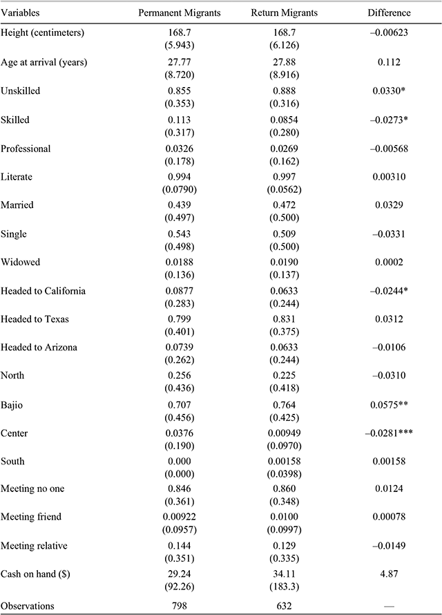
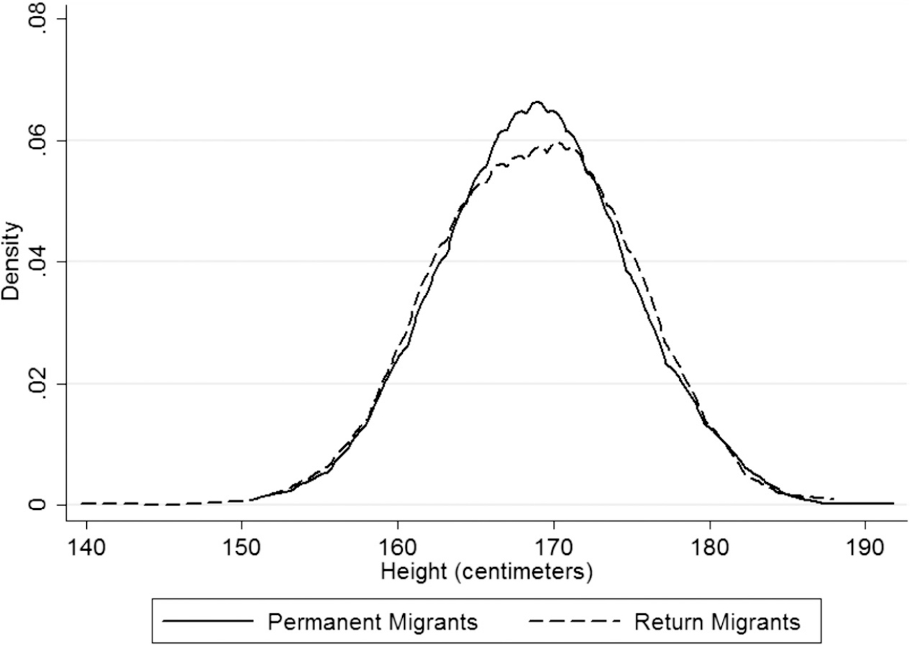
Despite the fact that permanent migrants and return migrants ended up in different countries, their characteristics upon arrival, as shown in Table 4, were remarkably similar. Return migrants and permanent migrants were statistically indistinguishable in terms of age, marital status, and cash on hand at arrival. Perhaps surprisingly, there was no difference in network connections, which could have supported migrants and altered return behavior. Importantly, there was also no statistically significant difference in heights, which suggests that return migrants were not differentially selected from the migrant population (see Figure 5).
Return migrants and permanent migrants were not similar in every way. Migrants born in the Center region were more likely to be permanent migrants, while those born in the Bajio region were more likely to be return migrants.Footnote 27 Those who listed their intended destination as California were least likely to become return migrants. The further distance between sending states and California likely increased the costs of returning, lowering return rates (Borjas and Bratsberg Reference Borjas and Bratsberg1996). In addition, return migrants were slightly more likely to be unskilled, although the magnitude of this difference is small and only marginally statistically significant. While the difference in occupational class suggests that return migrants were negatively selected on occupation, it is unknown whether occupation was intended or previous occupation, leaving their true position in the skill distribution unclear.
Summary Statistics for Permanent and Return Migrants

* = Significant at the 10 percent level.
** = Significant at the 5 percent level.
*** = Significant at the 1 percent level.
Notes:
Standard deviations are in parentheses. Proportions are reported unless otherwise noted. Permanent migrants are those migrants linked to the 1930 U.S. Census and return migrants are those linked to the 1930 Mexican Census.
Source:
Border crossing manifests.
Heights: Permanent and Return Migrants

Estimating Selection into Return Migration
We revisit the observation from Table 4 and Figure 5 that permanent and return migrants had similar heights (168.7 centimeters) and test whether this result holds when controlling for age and region of birth. Specifically, we pool the return and permanent migrant samples and regress height on an indicator for whether the migrant was a return migrant.
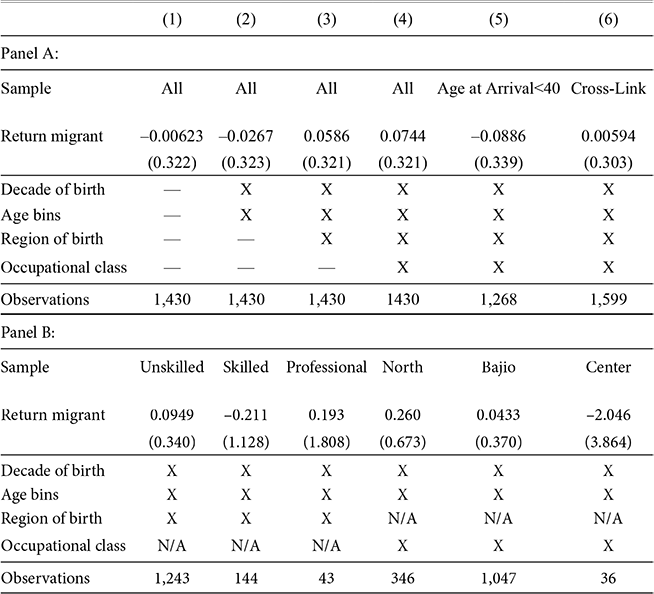
The results of the regression of height on return migration status are presented in Panel A of Table 5. A simple correlation in the first column shows that return migrants were 0.006 centimeters shorter than permanent migrants, a statistically and economically insignificant difference. In regressions including age and region of birth fixed effects, heights of return and permanent migrants continue to be statistically indistinguishable. Although occupational structures upon arrival were slightly different between return and permanent migrants, once controlling for occupational structure there was still no differential selection of return migrants. Panel B shows alternative sample specifications for samples including only unskilled, skilled, or professional workers, and also including only people born in the North, Bajio, or Center region. All regressions show no economically or statistically significant differences between return migrants and permanent migrants in terms of height. Overall, our analysis suggests that return migrants and permanent migrants had similar levels of human capital.
Regression Results for Return Selection

* = Significant at the 10 percent level.
** = Significant at the 5 percent level.
*** = Significant at the 1 percent level.
Notes:
Robust standard errors are in parentheses. The dependent variable in each regression is height. Each regression has different sample specifications. Permanent migrants are those migrants linked to the 1930 U.S. Census and return migrants are those linked to the 1930 Mexican Census.
Source:
Border crossing manifests.
Robustness of Results for the Linked Sample
Linked samples may not be representative of their underlying populations because the links are not made at random. Specifically, a migrant is more likely to be connected if he has a unique name, and he will not be linked if there was a death, name change, or transcription error. While transcription error was likely random with respect to height, name changes could have occurred more often for migrants intending to reside permanently in the United States. If those migrants were more adept at English or at acquiring United States specific human capital, then our linked sample would underestimate the quality of permanent migrants.
Another concern is that mortality might bias results if taller individuals are healthier and likely live longer. We restrict the sample to migrants arriving under the age of 40 who were less likely to die within ten years. The results, shown in Column (5) of Panel A of Table 5, indicate that even with the restricted sample we find no differential selection into return migration.
Lastly, it is possible that households in Mexico reported migrants in the United States as members of the household to enumerators. This error would imply that links to both the United States and Mexican censuses were actually people who resided in the United States. We include 169 migrants who were uniquely linked to both the United States Census and the Mexican Census in our sample of permanent migrants and regress height on return migrant status. The result reported in Column (6) in Panel A of Table 5 confirms that return migrants defined in this manner were not differentially selected from the population.
CONCLUSIONS
In the early twentieth century, the United States labor market drew the taller workers from Mexico. Mexican migrants were over four centimeters taller than members of the Mexican military and only one and a half centimeters shorter than passport holders. The fact that Mexican migrants were positively self-selected is consistent with Borjas (Reference Borjas1987) and Chiquiar and Hanson (Reference Chiquiar and Hanson2005) where migrants had high costs of travel or faced credit constraints, limiting the ability of lower-quality Mexicans to migrate. This positive self-selection represents a “quality drain” or “productivity drain” from Mexico to the United States.
From our linked sample we find that return migrants were not differentially selected. Taller individuals migrated from Mexico, and migrants observed years later in the United States were just as tall. Time and return migration did not impact the quality drain on Mexico or the quality gain to the United States that resulted from positive self-selection into migration from Mexico.
This lack of selection on height for Mexican return migrants is in contrast to negative self-selection of most European return migrants during the early 1900s (Abramitzky et al. Reference Abramitzky, Boustan and Eriksson2014).Footnote 28 It is possible that this result could be due to deportation or the threat of deportation, which forced different people out of the United States than would otherwise leave and thus likely altered the selection of return migrants. If the United States randomly deported Mexicans without respect to human capital or skill then this would lead to return migrants having the same human capital as permanent migrants, which we find. While purely economic forces might lead to the lowest performing migrants leaving the country, deportation policies expel both high- and low-quality migrants. However, other reasons (for example, proximity to Mexico) could also explain the different patterns in return migrant selection between Europeans and Mexicans.
A pattern of positive self-selection of Mexican migrants affects both Mexico and the United States in a variety of ways. The United States received the relatively more productive Mexican workers, and these workers would assimilate into the labor market more quickly than negatively selected migrants. For Mexico, the taller laborers, the taller miners, and the taller farmers left Mexico to work in the United States, draining Mexico of human capital and lowering the productivity of the average Mexican worker. However, the total effect on Mexican development is unclear as migration affects not only labor markets, but also can influence home country savings and investment by increasing remittances. It further affects the home country by changing political institutions if migrants return back home, by increasing technological diffusion with the transmission of techniques or capital goods across borders, or by influencing future migration with the strengthening of networks. This study provides a valuable step to better understanding the various effects of historical migration from Mexico to the United States on the economies of both nations.