





1 Introduction
Thermal transport is an important process in a range of plasma environments, ranging from high-energy-density physics (HEDP) and inertial confinement fusion (ICF) plasmas to the intra-cluster medium (ICM) of galaxy clusters. In the context of ICF, thermal conduction plays a pivotal role in the formation and evolution of the hot-spot, with heat conduction from the hot-spot to the surrounding cooler dense plasma, one of the primary loss mechanisms during burning fuel-capsule implosions[
1
]. Accurate modelling of heat transport is therefore essential for realizing successful ICF experiments; yet, classical models exhibit systematic discrepancies when compared with observations pointing to the role of kinetic processes[
Reference Rinderknecht, Amendt, Wilks and Collins
2
], while magnetic fields generated prior to the stagnation phase of ICF implosions may also significantly influence heat transport[
Reference Walsh, Chittenden, McGlinchey, Niasse and Appelbe
3
,
Reference Walsh and Clark
4
]. Recent studies have explored how imposed magnetic fields during ICF implosions could positively alter the properties of the fusing plasma[
Reference O’Neill, Appelbe, Crilly, Walsh, Strozzi, Moody and Chittenden
5
,
Reference Walsh, Strozzi, Povilus, O’Neill, Leal, Pollock, Sio, Hammel, Djordjević, Chittenden and Moody
6
]. For instance, introducing a magnetic field across the fuel-capsule prior to implosion has been shown to increase ion temperatures by up to
$40\%$
 and neutron yields by more than threefold, relative to unmagnetized shots of similar drive energy[
Reference Chang, Fiksel, Hohenberger, Knauer, Betti, Marshall, Meyerhofer, Séguin and Petrasso
7
,
Reference Moody, Pollock, Sio, Strozzi, Ho, Walsh, Kemp, Lahmann, Kucheyev, Kozioziemski, Carroll, Kroll, Yanagisawa, Angus, Bachmann, Bhandarkar, Bude, Divol, Ferguson, Fry, Hagler, Hartouni, Herrmann, Hsing, Holunga, Izumi, Javedani, Johnson, Khan, Kalantar, Kohut, Logan, Masters, Nikroo, Orsi, Piston, Provencher, Rowe, Sater, Skulina, Stygar, Tang, Winters, Zimmerman, Adrian, Chittenden, Appelbe, Boxall, Crilly, O’Neill, Davies, Peebles and Fujioka
8
]. These results suggest that external magnetic fields can significantly enhance the performance of ICF experiments.
Thermal conduction is also thought to play a key role in one of the longest-standing puzzles in the physics of the ICM: the cooling-flow problem[ Reference Fabian 9 ]. Observed luminosity and density profiles from galaxy cluster cores and the surrounding ICM suggest that radiative cooling times should be much shorter than the Hubble time, a discrepancy that has been a central issue in the field for several decades[ Reference Lea, Silk, Kellogg and Murray 10 – Reference Cowie and Binney 12 ]. Such radiative losses would, in principle, drive mass accretion onto the cooling cores to maintain pressure balance with the gravitational potential of the surrounding gas. This could initiate a feedback loop in which radiative core cooling is followed by the inflow of cooling material onto the cluster’s core. The result would be cooling instabilities, which in turn would yield mass deposition and stellar formation rates that are much greater than what is observed. Despite evidence of cooling flows, key dynamical properties of clusters with cooling cores – for example, the mass deposition rate, central cooling time and central entropy – have remained approximately constant over several Gyr[ Reference McDonald, Benson, Vikhlinin, Stalder, Bleem, de Haan, Lin, Aird, Ashby, Bautz, Bayliss, Bocquet, Brodwin, Carlstrom, Chang, Cho, Clocchiatti, Crawford, Crites, Desai, Dobbs, Dudley, Foley, Forman, George, Gettings, Gladders, Gonzalez, Halverson, High, Holder, Holzapfel, Hoover, Hrubes, Jones, Joy, Keisler, Knox, Lee, Leitch, Liu, Lueker, Luong-Van, Mantz, Marrone, McMahon, Mehl, Meyer, Miller, Mocanu, Mohr, Montroy, Murray, Nurgaliev, Padin, Plagge, Pryke, Reichardt, Rest, Ruel, Ruhl, Saliwanchik, Saro, Sayre, Schaffer, Shirokoff, Song, Suhada, Spieler, Stanford, Staniszewski, Stark, Story and van Engelen 13 , Reference McDonald, Gaspari, McNamara and Tremblay 14 ]. The lack of evolution indicates a need for a thermal balance to keep the cluster cores and ICM in equilibrium. Active galactic nuclei (AGN) feedback from the cluster galaxies is thought to be the dominant source of this heating[ Reference Fabian 15 , Reference Ruppin 16 ], with the role of thermal conduction remaining a challenge in understanding the thermodynamics of the ICM. It has been predicted that thermal conduction needs to be suppressed to prevent cool-cores from isothermalizing without the need for fine tuning[ Reference Conroy and Ostriker 17 ], with the observation of persistent cold fronts similarly requiring this[ Reference ZuHone and Roediger 18 ]. The presence of tangled magnetic-field lines within the ICM suggests that various mechanisms could underlie this suppression[ Reference Kempf and Rincon 19 ], with significant implications for the efficacy of thermal balancing attributed to thermal conduction into the cluster core[ Reference Kunz, Schekochihin, Cowley, Binney and Sanders 20 ].
In collisional plasmas where the Coulomb mean-free paths of electrons and ions,
${\lambda}_\mathrm{e}$
 and
${\lambda}_\mathrm{i}$
 , are much smaller than the characteristic temperature length scale
${L}_{\mathrm{T}}$
 , it is possible to derive analytical expressions for the thermal conductivity using kinetic theory: the so-called ‘classical models’. In unmagnetized plasmas where the electron Larmor frequency
${\Omega}_\mathrm{e}$
 and the electron–ion collision time
${\tau}_\mathrm{ei}$
 satisfy
${\Omega}_\mathrm{e}{\tau}_\mathrm{ei}\ll 1$
 , such calculations yield the Spitzer model, in which heat flows down temperature gradients in the plasma, carried predominantly by electrons[
Reference Spitzer and Härm
21
,
Reference Cohen, Spitzer and Routly
22
]. The Spitzer heat flux
${q}_\mathrm{S}$
 is directly proportional to
${\tau}_\mathrm{ei}$
 , and has a strong dependence on the electron temperature:
${q}_\mathrm{S}\sim {m}_\mathrm{e}{n}_\mathrm{e}{v}_{\mathrm{the}}^4{\tau}_\mathrm{ei}/{L}_{\mathrm{T}}\propto {T}_\mathrm{e}^{7/2}$
 , where
${m}_\mathrm{e}$
 is the electron mass,
${n}_\mathrm{e}$
 is the electron number density,
${v}_{\mathrm{the}}$
 is the thermal electron velocity and
${T}_\mathrm{e}$
 is the electron temperature. In a collisional plasma with a temperature gradient that is strongly magnetized (
${\Omega}_\mathrm{e}{\tau}_\mathrm{ei}\gg 1$
 ), it can be shown that, compared with its parallel component
${q}_{\Vert }$
 , the heat flux in the direction perpendicular to the magnetic field
${q}_{\perp }$
 will be strongly suppressed:
${q}_{\perp }/{q}_{\Vert}\sim {\left({\Omega}_\mathrm{e}{\tau}_\mathrm{ei}\right)}^{-2}\ll 1$
 [
Reference Braginskii
23
]. The parallel heat flux is still given by the Spitzer model, with
${q}_{\Vert}\propto {T}_\mathrm{e}^{7/2}$
 .
However, the plasmas present in both the ICF hot-spot and the ICM are only weakly collisional, with important ramifications for modelling thermal transport. The Coulomb mean-free paths
${\lambda}_\mathrm{e}$
 and
${\lambda}_\mathrm{i}$
 are only a few orders of magnitude smaller than
${L}_{\mathrm{T}}$
 , and their thermal pressure
$p$
 is much larger than their magnetic pressure
${p}_\mathrm{B}$
 , resulting in a large plasma
$\beta \equiv p/{p}_\mathrm{B}$
 . Plasmas with these two characteristics, which also include other notable astrophysical and high-energy density (HED) settings such as the warm intergalactic medium[
Reference Nicastro, Mathur and Elvis
24
] and laser-ablated plasma[
Reference Tzeferacos, Rigby, Bott, Bell, Bingham, Casner, Cattaneo, Churazov, Emig, Fiuza, Forest, Foster, Graziani, Katz, Koenig, Li, Meinecke, Petrasso, Park, Remington, Ross, Ryu, Ryutov, White, Reville, Miniati, Schekochihin, Lamb, Froula and Gregori
25
–
Reference Meinecke, Tzeferacos, Ross, Bott, Feister, Park, Bell, Blandford, Berger, Bingham, Casner, Chen, Foster, Froula, Goyon, Kalantar, Koenig, Lahmann, Li, Lu, Palmer, Petrasso, Poole, Remington, Reville, Reyes, Rigby, Ryu, Swadling, Zylstra, Miniati, Sarkar, Schekochihin, Lamb and Gregori
27
], are expected to be susceptible to anisotropy-driven kinetic-scale instabilities when
${\lambda}_\mathrm{e}/{L}_{\mathrm{T}}\gtrsim 1/\beta$
 [
Reference Bott, Cowley and Schekochihin
28
]. These instabilities mean that classical models for heat conduction in magnetized plasma, which assume that heat transport is mediated only by Coulomb collisions, are inaccurate when the plasma is weakly collisional with a sufficiently large plasma
$\beta$
 [
Reference Choudhury and Bott
29
].
During the last few decades, various new models of thermal conductivity that incorporate the effect of kinetic instabilities have been put forward. Levinson and Eichler[ Reference Levinson and Eichler 30 ] proposed that the whistler heat-flux instability could affect heat transport once the amplitude of instability-driven magnetic fluctuations become large enough. The whistler heat-flux instability arises when a temperature-gradient-driven electron heat flux provides a source of free energy for the growth of whistler waves. As these waves grow to sufficiently large amplitudes, they can resonantly interact with heat-carrying electrons, leading to pitch-angle scattering and thereby modifying the electron distribution function. Various analytical[ Reference Pistinner and Eichler 31 – Reference Lopez, Bott and Schekochihin 33 ] and numerical studies[ Reference Roberg-Clark, Drake, Reynolds and Swisdak 34 – Reference Yerger, Kunz, Bott and Spitkovsky 37 ] have carried out further research on the instability, confirming that anomalous scattering causes a reduction in the parallel heat flux relative to the Spitzer value. For example, Komarov et al. [ Reference Komarov, Schekochihin, Churazov and Spitkovsky 35 ] reported the following:

This expression indicates that if
${\lambda}_\mathrm{e}/{L}_{\mathrm{T}}\gg 1/{\beta}_\mathrm{e}$
 , the parallel heat flux will be strongly suppressed, and become independent of the magnitude of the temperature gradient. Another model, appropriate for any kinetic instability that generates magnetic fluctuations with an amplitude comparable to the background magnetic-field strength, was proposed by Ryutov et al.
[
Reference Ryutov, Drake, Kane, Liang, Remington and Wood-Vasey
38
]:
${q}_{\Vert \mathrm{eff}}\sim {q}_{\perp \mathrm{eff}}\sim {\mathrm{\ell}}_{\delta B}{m}_\mathrm{e}{n}_\mathrm{e}{v}_{\mathrm{the}}^3/2{L}_{\mathrm{T}}\sim {q}_\mathrm{S}{\mathrm{\ell}}_{\delta B}/{\lambda}_\mathrm{e}$
 , where
${\mathrm{\ell}}_{\delta B}$
 is the correlation scale of the magnetic perturbations. In this model, conduction is quasi-isotropic, even though the Larmor radius
${\rho}_\mathrm{e}\ll {\lambda}_\mathrm{e}$
 , but is still proportional to the temperature gradient. Although in specific contexts these models have been validated[
Reference Yerger, Kunz, Bott and Spitkovsky
37
], their applicability more generally in weakly collisional plasmas remains uncertain.
Advancements made in kilojoule to megajoule and petawatt laser facilities[
Reference Danson, Bromage, Butcher, Chanteloup, Chowdhury, Galvanauskas, Gizzi, Haefner, Hein, Hillier, Hopps, Kato, Khazanov, Kodama, Korn, Li, Li, Limpert, Ma, Nam, Neely, Papadopoulos, Penman, Qian, Rocca, Shaykin, Siders, Spindloe, Szatmári, Trines, Zhu, Zhu and Zuegel
39
], such as the National Ignition Facility (NIF) and the OMEGA laser at the Laboratory for Laser Energetics (LLE), have made laboratory investigations of heat transport in weakly collisional, magnetized plasma possible. Although experiments investigating the effect of non-locality[
Reference Henchen, Sherlock, Rozmus, Katz, Cao, Palastro and Froula
40
] and magnetic fields[
Reference Froula, Ross, Pollock, Davis, James, Divol, Edwards, Offenberger, Price, Town, Tynan and Glenzer
41
] on heat transport in laser plasmas are well established, recent experiments reported by Meinecke et al.
[
Reference Meinecke, Tzeferacos, Ross, Bott, Feister, Park, Bell, Blandford, Berger, Bingham, Casner, Chen, Foster, Froula, Goyon, Kalantar, Koenig, Lahmann, Li, Lu, Palmer, Petrasso, Poole, Remington, Reville, Reyes, Rigby, Ryu, Swadling, Zylstra, Miniati, Sarkar, Schekochihin, Lamb and Gregori
27
] represent a significant step forward in this regard, providing evidence for suppressed heat conduction compared with classical models in a turbulent, magnetized, weakly collisional plasma. In these experiments, which were carried out on the NIF, temperature fluctuations of characteristic scale
${L}_\mathrm{T}\gtrsim 5{\lambda}_\mathrm{e}$
 were observed to persist for hundreds of classical thermal diffusion times, consistent with a suppressed conduction compared to the Spitzer model by around two orders of magnitude. This suppression was linked to electron magnetization by comparing the NIF experimental results with the conduction characteristics of turbulent plasmas created in experiments at the OMEGA Laser Facility[
Reference Tzeferacos, Rigby, Bott, Bell, Bingham, Casner, Cattaneo, Churazov, Emig, Fiuza, Forest, Foster, Graziani, Katz, Koenig, Li, Meinecke, Petrasso, Park, Remington, Ross, Ryu, Ryutov, White, Reville, Miniati, Schekochihin, Lamb, Froula and Gregori
25
,
Reference Bott, Tzeferacos, Chen, Palmer, Rigby, Bell, Bingham, Birkel, Graziani, Froula, Katz, Koenig, Kunz, Li, Meinecke, Miniati, Petrasso, Park, Remington, Reville, Ross, Ryu, Ryutov, Séguin, White, Schekochihin, Lamb and Gregori
26
] which, besides smaller values of
${\Omega}_\mathrm{e}{\tau}_\mathrm{ei}$
 comparatively, were physically similar. Suppressed conduction was only observed when
${\Omega}_\mathrm{e}{\tau}_\mathrm{ei}\gg 1$
 , for the NIF produced plasma: experiments in which
${\Omega}_\mathrm{e}{\tau}_\mathrm{ei}\lesssim 1$
 yielded smooth temperature profiles despite exhibiting comparable turbulent velocity statistics. However, beyond this correlation, the suppression mechanism was not well constrained, with various different possibilities plausibly operating: non-local effects, the trapping of heat-carrying electrons by magnetic mirrors[
Reference Komarov, Churazov, Kunz and Schekochihin
42
] and predominantly orthogonal arrangements of temperature gradients and magnetic fields[
Reference Komarov, Churazov, Schekochihin and ZuHone
43
] as well as whistler heat-flux instabilities. Testing specific conduction models in such a complex plasma environment – in particular, one with a highly stochastic magnetic field – is a significant challenge.
To overcome this challenge, we have designed a new experimental platform to be fielded on the Orion laser facility[
Reference Hopps, Oades, Andrew, Brown, Cooper, Danson, Daykin, Duffield, Edwards, Egan, Elsmere, Gales, Girling, Gumbrell, Harvey, Hillier, Hoarty, Horsfield, James, Leatherland, Masoero, Meadowcroft, Norman, Parker, Rothman, Rubery, Treadwell, Winter and Bett
44
], which produces a magnetized, high-
$\beta$
 , weakly collisional plasma with temperature gradients directed along embedded magnetic-field lines with a simple geometry. The goal of this platform is to characterize thermal conduction in a plasma susceptible to whistler heat-flux instabilities for comparison against a range of different heat conduction models. This paper contains a description of the new experimental platform, as well as a series of complementary simulations using the radiation-magnetohydrodynamics (MHD) code FLASH[
Reference Fryxell, Olson, Ricker, Timmes, Zingale, Lamb, MacNeice, Rosner, Truran and Tufo
45
], and also synthetic diagnostic data. The simulations were run with various conduction models supported by FLASH to investigate how the evolution of the plasma is affected by thermal conductivity. Our key finding is that the evolution of the temperature profile is dependent primarily on the heat conduction model, suggesting the temperature measurements will provide significant constraints on the thermal conductivity.
The remainder of this paper is structured as follows. Section 2 describes the design overview of the platform, with descriptions of the target and previous iterations of the design alongside FLASH simulation outputs of the resulting plasma. Section 3 discusses the three primary diagnostics to be fielded throughout the campaign, with analysis of synthetic data produced for each diagnostic. Finally, Section 4 discusses the evolution of a set of notable plasma parameters relevant to the problem, and how the thermodynamics compare between the three conduction models.
2 Design overview
To produce a magnetized, weakly collisional, high-
$\beta$
 plasma with temperature gradients directed along magnetic-field lines such that the whistler heat-flux instability can grow, we propose the experimental design illustrated in Figure 1. A front-side blow-off plasma is produced by ablating a foil with multiple drive lasers, expanding from the target in an approximate hemispherical plume with radius parallel to the foil normal. The supersonic blow-off plasma then collides with a secondary ‘shock’ foil with its plane face normal to that of the drive foil. The resulting shock wave in the plasma jet will convert the majority of its kinetic energy into thermal energy, resulting in a subsonic planar plasma[
Reference Ben-Dor, Igra and Elperin
46
,
Reference Colvin and Larsen
47
] whose properties are amenable for the operation of the whistler heat-flux instability ; by contrast, without this shock heating and magnetic-field amplification the whistler heat-flux instability cannot grow. Pressure gradients in the central blow-off plume, which are tuned by the laser spot separation, generate temperature gradients in the shocked plasma from the central dense planar region to the less dense wings towards the edges of the shock foil. The plasma’s magnetic field is generated by the Biermann battery mechanism operating on misaligned density and temperature gradients present in the front-side blow-off plasma[
Reference Biermann
48
–
Reference Stamper and Ripin
50
]. This plasma has a large magnetic Reynolds number, so the magnetic field is advected with the blow-off plasma as it expands[
Reference Alfvén and Mat
51
]. Although this expansion also dilutes the magnetic-field strength, as the field passes through the shock wave, its component perpendicular to the shock normal is re-amplified, resulting in a magnetic field in the planar plasma whose orientation is primarily in the plane of the shock foil.
Simplified conceptualization of the experimental design. Firstly, driving of the target (drive) foil produces a front-side blow-off plasma. Then, on collision of that front-side blow-off plasma with a secondary shock foil, oriented orthogonally to the drive foil, a shocked plasma, threaded with self-generated magnetic fields parallel to the temperature gradients created during the drive foil’s ablation, is created. The shocked plasma’s production is illustrated from both the front and side views of the target.

Figure 1 Long description
Panel one, labeled ‘Front view 1’, shows two blue drive beams converging on a gray drive foil, with a gray shock foil below. Panel two, labeled ‘Front view 2’, shows the drive foil with a curved orange region labeled ‘Plasma’ expanding downward toward the shock foil. Purple lines labeled ‘B’ run parallel to the shock front, which is marked in red. An orange arrow labeled ‘gradient parallel T sub e’ points leftward along the plasma boundary. Panel three, labeled ‘Side view 1’, shows the beams are striking the drive foil from the right, with the shock foil positioned below. Panel four, labeled ‘Side view 2’, shows the drive foil and shock foil with a red shock front arching over an orange plasma region. Purple lines labeled ‘B’ curve above the plasma traveling in the direction normal to plane of the page (towards the reader), and an orange arrow labeled ‘gradient parallel T sub e’ points outwards towards the reader. The sequence illustrates the generation of a blow-off plasma by the drive beams, its collision with the shock foil, and the formation of a shocked plasma threaded by self-generated magnetic fields aligned with the temperature gradient.
The temperature, density, magnetic-field strength and temperature gradient scale
${L}_{\mathrm{T}}$
 in the shocked planar plasma can be tuned to access the regime of interest by varying the intensity of drive lasers, their spot profile and the separation of the drive and shock foils. For the whistler heat-flux instability to operate at all, we require that
${L}_{\mathrm{T}}/{\lambda}_\mathrm{e}\lesssim {\beta}_\mathrm{e}$
 within the planar plasma, and the Hall parameter
${\mathrm{Ha}}_\mathrm{e}\equiv {\lambda}_\mathrm{e}/{\rho}_\mathrm{e}$
 to satisfy
${\mathrm{Ha}}_\mathrm{e}\gtrsim 1$
 . We also require both the characteristic e-folding timescale
${\tau}_{\mathrm{lin}}\sim {L}_{\mathrm{T}}/{\lambda}_\mathrm{e}{\Omega}_\mathrm{e}$
 of the whistler heat-flux instability and the timescale
${\tau}_{\mathrm{c}}\sim {L}_\mathrm{T}/{\beta}_\mathrm{e}{v}_{\mathrm{the}}$
 , over which the amplified whistlers scatter electrons to be much smaller than the dynamical timescale
${\tau}_{\mathrm{dyn}}$
 over which the temperature gradient evolves[
Reference Bott, Cowley and Schekochihin
28
,
Reference Komarov, Schekochihin, Churazov and Spitkovsky
35
]. To ascertain under which platform design parameters the relevant conditions were obtained, we carried out several simulation campaigns using the FLASH plasma-fluid simulation code. FLASH[
Reference Fryxell, Olson, Ricker, Timmes, Zingale, Lamb, MacNeice, Rosner, Truran and Tufo
45
] is a publicly available Eulerian, finite-volume radiation-MHD code with extensive HEDP capabilities[
Reference Tzeferacos, Fatenejad, Flocke, Graziani, Gregori, Lamb, Lee, Meinecke, Scopatz and Weide
52
], making use of the equation of state (EoS) and opacity tables from PrOpacEoS[
Reference MacFarlane, Golovkin and Woodruff
53
]. This makes it a reliable tool for the simulation of laser–plasma experiments, validated against a range of high-power laser–plasma experiments[
Reference Tzeferacos, Rigby, Bott, Bell, Bingham, Casner, Cattaneo, Churazov, Emig, Fiuza, Forest, Foster, Graziani, Katz, Koenig, Li, Meinecke, Petrasso, Park, Remington, Ross, Ryu, Ryutov, White, Reville, Miniati, Schekochihin, Lamb, Froula and Gregori
25
,
Reference Bott, Tzeferacos, Chen, Palmer, Rigby, Bell, Bingham, Birkel, Graziani, Froula, Katz, Koenig, Kunz, Li, Meinecke, Miniati, Petrasso, Park, Remington, Reville, Ross, Ryu, Ryutov, Séguin, White, Schekochihin, Lamb and Gregori
26
,
Reference Tzeferacos, Fatenejad, Flocke, Graziani, Gregori, Lamb, Lee, Meinecke, Scopatz and Weide
52
,
Reference Fatenejad, Bell, Benuzzi-Mounaix, Crowston, Drake, Flocke, Gregori, Koenig, Krauland, Lamb, Lee, Marques, Meinecke, Miniati, Murphy, Park, Pelka, Ravasio, Remington, Reville, Scopatz, Tzeferacos, Weide, Woolsey, Young and Yurchak
54
–
Reference Moczulski, Wen, Campbell, Scopatz, Palmer, Bott, Arrowsmith, Beyer, Blazevic, Bagnoud, Feister, Halliday, Karnbach, Metternich, Nazary, Neumayer, Reyes, Hansen, Schumacher, Spindloe, Sarkar, Bell, Bingham, Miniati, Schekochihin, Reville, Lamb, Gregori and Tzeferacos
62
].
2.1 Target design
The initial phase of the target’s design process involved finding appropriate choices for the characteristics of the drive and shock foils, as well as a long-pulse (LP) beam geometry appropriate to be fielded on the Orion Laser Facility[
Reference Hopps, Oades, Andrew, Brown, Cooper, Danson, Daykin, Duffield, Edwards, Egan, Elsmere, Gales, Girling, Gumbrell, Harvey, Hillier, Hoarty, Horsfield, James, Leatherland, Masoero, Meadowcroft, Norman, Parker, Rothman, Rubery, Treadwell, Winter and Bett
44
]. Each LP beam on Orion delivers up to
$400$
 J at a wavelength of
$351$
 nm. A previous experiment carried out on the facility focused each LP beam onto separate approximately 250 μm diameter spots on chlorine-doped millimetre-scale CH targets using a
$1$
 ns square pulse and obtained weakly collisional front-side blow-off plasmas with values of
$\beta \sim 1$
 –
$100$
 and
${\mathrm{Ha}}_\mathrm{e}\sim 10$
 [
Reference Tubman, Joglekar, Bott, Borghesi, Coleman, Cooper, Danson, Durey, Foster, Graham, Gregori, Gumbrell, Hill, Hodge, Kar, Kingham, Read, Ridgers, Skidmore, Spindloe, Thomas, Treadwell, Wilson, Willingale and Woolse
63
]. Such values are appropriate for our proposed study, suggesting that irradiating millimetre-scale drive and shock chlorine-doped CH foils using Orion’s LP beams in a similar manner would be a productive basis for the platform.
To refine the design, a series of three-dimensional (3D) FLASH simulations were performed, using a flux-based (explicit) Biermann battery and isotropic magnetic resistivity as extended MHD terms[
Reference Tzeferacos, Fatenejad, Flocke, Graziani, Gregori, Lamb, Lee, Meinecke, Scopatz and Weide
52
,
Reference Tzeferacos, Rigby, Bott, Bell, Bingham, Casner, Cattaneo, Churazov, Emig, Flocke, Fiuza, Forest, Foster, Graziani, Katz, Koenig, Li, Meinecke, Petrasso, Park, Remington, Ross, Ryu, Ryutov, Weide, White, Reville, Miniati, Schekochihin, Froula, Gregori and Lamb
55
], investigating different configurations. Other extended MHD terms, in particular the Nernst term, were not used, because they are suppressed by the large Hall parameter in the plasma of interest (see Section 4). In each of the simulations, the appropriate material properties of chlorine-doped CH targets were used, as well as the LP beam parameters described in the previous paragraph (see Figure 2). During the campaigns, the simulation domain was a fixed uniform resolution,
${256}^3$
 Cartesian grid of resolution
$\Delta x=\Delta y=\Delta z=1\times {10}^{-3}$
 cm. Here, the
$x$
 direction is that normal to the drive foil, the
$z$
 direction is normal to the shock foil and the
$y$
 direction is the third orthogonal direction. The origin of the domain was centred such that
$-0.2021$
 cm
$\le x\le 0.0721$
 cm,
$-0.1276$
 cm
$\le y\le 0.1276$
 cm and
$-0.2021$
 cm
$\le z\le 0.0721$
 cm. Outflow boundary conditions were utilized in all simulations. The first design used five drive beams directed normal to the plane of the drive foil (Figure 2(a)) and a shock foil that extended 2 mm in the direction anti-parallel to the drive beam propagation axis. This produced a weakly collisional, high-
$\beta$
 plasma with parameters generally compatible with operation of the whistler heat-flux instability. However, the extended length of the shock foil caused issues: partial reflection and scattering of the drive beams by the front-side blow-off plasma ablated its end (Figure 2(a)). This ablation did not affect the planarity of the shocked plasma directly below the drive foil. However, magnetic fields oriented opposite to those in the bulk of the planar plasma were produced in the ablated shock foil, significantly distorting path-integrated measurements of magnetic fields. Because the extended length yielded no apparent benefits, a new design with a shorter shock foil was an obvious improvement.
Evolution of the target design. (a) Original five-beam proof-of-concept visualization with all drive beams normal to target. The left-hand side shows all beams incident on the drive foil, and the resultant ablation plume on the right-hand side, with the end of the shock foil ablating prior to contact with the jet plasma. (b) Updated four-beam design visualization using the Orion chamber beam alignment geometry and a shorter shock foil. The top right-hand panel shows the target top-down and the bottom right-hand panel shows the target side-on, matching the line of sight (LoS) seen in the top and bottom rows, respectively, of (c). (c) 2D slices taken from the FLASH simulation data for
${T}_\mathrm{e}$
 (left) and
${n}_\mathrm{e}$
 (right) for
$z=-0.114$
 cm (top row) and
$y=0$
 cm (bottom row) at
$t=1.5$
 ns post the drive-foil ablation. (d) Same as (b), but with the final two-beam configuration. (e) Comparison of 2D slices from FLASH simulation data for
${T}_\mathrm{e}$
 (top row) and
${n}_\mathrm{e}$
 (bottom row), as in (c) for the two-beam and four-beam design, indicating the more laminar nature of the temperature and density profiles for the two-beam design.

Figure 2 Long description
Panel a shows two 3D renderings. The left subpanel displays red vectors representing five beams incident perpendicularly on a drive foil, with a shock foil below, axes labeled x, y, z. The right subpanel shows a gray ablation plume expanding from the drive foil toward the shock foil. Panel b presents the four-beam design: the left subpanel is a top-down schematic with blue cones labeled L P 8, L P 10, L P 6, L P 2 converging on the drive foil and shock foil; the right subpanels show side and end views of the shock foil with blue cones indicating beam paths. Panel c contains six color-mapped 2D slices from FLASH simulation data. The top row shows electron temperature T sub e, magnetic field B sub y, and electron density n sub e at z equals negative zero point one one four centimeters, t equals one point five nanoseconds. The bottom row shows the same variables at y equals zero centimeters. Color bars indicate value ranges. Panel d shows the final two-beam design, with the left subpanel a top-down schematic of L P 2 and L P 6 beams converging on the drive and shock foils, and right subpanels showing side and end views with blue cones. Panel e compares 2D FLASH simulation slices for the original and updated designs: the top row shows T sub e, the bottom row shows n sub e, with more laminar profiles in the updated design. All axes and color bars are labeled, and spatial relationships between beams, foils, and simulation outputs are maintained.
Using the shortened platform, the beam profiles and angles of incidence were then updated to more accurately represent the capabilities of the Orion facility[
Reference Hopps, Oades, Andrew, Brown, Cooper, Danson, Daykin, Duffield, Edwards, Egan, Elsmere, Gales, Girling, Gumbrell, Harvey, Hillier, Hoarty, Horsfield, James, Leatherland, Masoero, Meadowcroft, Norman, Parker, Rothman, Rubery, Treadwell, Winter and Bett
44
]. The number of beams was reduced to four because of geometric feasibility, making use of LP beams 2, 6, 8 and 10 (see Figure 2(b)). This update highlighted the importance of accurate modelling of the angle of incidence of the drive beams with respect to the drive foil. The incidence of LP-8 and LP-10 onto the drive foil from above the plane of its normal led to worsened scattering of laser light onto the shock foil compared with previous five-beam design, a feature that even the shortened platform could not avoid. Although the resulting plasma was again weakly collisional, and with high-
$\beta$
 , this scattered light generated non-planar features in the temperature and density profiles of the shocked plasma (Figure 2(c)); pronounced stochasticity in its magnetic fields was also observed. Both features prohibited use of LP-8 and LP-10 in this platform.
To avoid this issue, a new two-beam design using only LP-2 and LP-6 was considered (Figure 2(d)). This design avoided any ablation of the drive foil by scattered laser light, resulting in a genuinely planar, weakly collisional, high-
$\beta$
 plasma suitable for our experiment of interest (Figure 2(e)). In this new design, the separation
${L}_{\mathrm{spots}}$
 between the spots was then tuned to control the horizontal size of the planar plasma, while avoiding any magnetic reconnection effects in the drive foil (see Section 2.2). The distance
${L}_{\mathrm{shock}}$
 of the shock foil from the drive foil was chosen via a simple optimization: too close, and the curvature of the blow-off plasma causes departures from planarity; too far, and the plasma density becomes too low to be easily detectable.
A detailed visualization of the target to be fielded with the two-beam design is shown in Figure 3. The drive and shock foils consist of
$1.6$
 mm
$\times$
 $0.75$
 mm
$\times$
 $0.2$
 mm and
$1.2$
 mm
$\times$
 $0.75$
 mm
$\times$
 $0.2$
 mm slabs of parylene C (
$50\%$
 C,
$43.75\%$
 H,
$6.25\%$
 Cl) and plastic (
$50\%$
 C,
$50\%$
 H), respectively, separated by a
$0.8$
 mm gap between the bottom of the drive foil and the top face of the shock foil. To maximize target stability, the foils are slotted into a 3D printed ‘chair’, in turn mounted on a machined aluminium (Al) block.
(a) Top-down VisRad visualization of the experimental configuration within the Orion chamber. The drive and shock foils are placed in the centre of the chamber with the plane face of the shock foil facing out of the page, and the plane face of the drive foil facing northward. The LP drive beams are shown in blue targeting the drive foil, with the SP beams shown in red targeting the Au foils for proton production. The diagnostic detectors are off-screen with their radial position, relative to target chamber centre (TCC), with LoSs indicated by the orange arrows. The slit foil at the bottom of the image is to screen the X-rays for the spectrometer, which will be swapped out mid-way through the campaign to be replaced with a spatially resolved GXD. (b) Target configuration on the Al mounting block. The orange chair will be 3D printed with the drive and shock foils mounted on it. The cross-beam structure holding the chair will increase stability and ensure that the drive and shock foils’ plane faces will remain orthogonal post ablation. The polar and azimuthal angles for the LP and SP drive beams are described in Ref. [Reference Hopps, Oades, Andrew, Brown, Cooper, Danson, Daykin, Duffield, Edwards, Egan, Elsmere, Gales, Girling, Gumbrell, Harvey, Hillier, Hoarty, Horsfield, James, Leatherland, Masoero, Meadowcroft, Norman, Parker, Rothman, Rubery, Treadwell, Winter and Bett44].

Figure 3 Long description
Panel a is a top-down schematic centered on the intersection of x and y axes, marking the chamber center. At the center are the drive and shock foils, with the shock foil’s plane facing out of the page and the drive foil’s plane facing north. Blue sectors represent L P drive beams (500 J, 1 nanosecond pulse, lambda equals 351 nanometers) coming from the north-west and north-east, respectively, in this orientation. Red sectors represent S P beams (500 to 200 J, 0.5 picosecond pulse, lambda equals 1054 nanometers) targeting gold foils for proton production from the northwest and southwest. Orange arrows indicate lines of sight for diagnostic detectors labeled G X D and R C F stack at 130 millimeters, radiating outward from the center. The slit foil is positioned at the southern edge, screening X-rays for the spectrometer or G X D. All distances from the center to SP driven foils are marked as 6 millimeters. Panel b is a 3D schematic anchored at the target mount. The orange chair structure holds the drive foil (top) and shock foil (below), ensuring their planes remain orthogonal. Blue L P beams (L P 2 and L P 6) are directed at the drive foil, while red S P beams (S P 1 and S P 2) target gold foils with shields and beam blocks. The slit foil is shown at the left, and the mounting block supports the entire assembly. The spatial arrangement ensures precise alignment for beam incidence and diagnostic access.
In addition to the main target, various additional components are mounted onto the Al block to facilitate diagnostics. The mounting block supports an adjustable
$10.6$
 mm
$\times$
 $2.0$
 mm
$\times$
 $0.2$
 mm Al sheet, containing a
$0.8$
 mm
$\times$
 $0.3$
 mm vertical slit, to set the resolution of the X-ray spectrometer (see Section 3.2). This sheet is positioned with its plane face normal to the rear side of the target chair,
$5.85$
 mm away. It is set such that only the area between the drive and shock foils is visible to the spectrometer. In addition, two circular gold (Au) foils are fastened to the mounting block, from which proton beams for imaging will be generated using Orion’s short-pulse (SP) beams. The foils are 0.05 mm thick, have
$1.1$
 and
$2.4$
 mm diameters, and are
$6$
 mm away from the centre of the chair, at angles of
${30}^{\circ }$
 and
${135}^{\circ }$
 counter clockwise relative to the normal of the drive foil’s face, respectively. They are centred at
$0.15$
 mm above the shock foil. Protective cylinders,
$1$
 and
$2$
 mm long with an inner diameter of
$1$
 mm, are used to shield the Au foils to prevent pre-ablation to the foil surface for the
$30{}^{\circ}$
 and
$135{}^{\circ}$
 foils. Beam blockers are mounted on the frame containing the Au foils, placed at an angle of
$68{}^{\circ}$
 normal to the foil plane, to prevent reflection of the SP beam into the parabola of the adjacent SP beam. The expected on-target intensity of the drive beams is
$6\times {10}^{14}$
 W cm
${}^{-2}$
 horizontally separated by
$0.5\ \mathrm{mm}$
 . The SP beams each deliver
$5\times {10}^{20}$
 W cm
${}^{-2}$
 to their respective target, containing up to
$500$
 J over a
$5\times {10}^{-4}$
 ns pulse at a wavelength of
$1054$
 nm. The LPs will have super-Gaussian beam profiles, shaped by phase plates to create circular on-target profiles with
$230\ \mu \mathrm{m}$
 focal spot size, while the SPs have an approximate focal spot size of
$7.7\ \mu \mathrm{m}$
 .
2.2 Simulated plasma parameters
One key benefit of designing a new experimental platform using a plasma simulation code such as FLASH is the possibility of detailed characterizations of the plasma conditions realized, and their sensitivity to different models of conduction. In this section, we explore the evolution of temperature, density and magnetic fields in three different simulations of the final two-beam design that employed different conduction models: the flux-limited Spitzer, Ryutov and no conduction. When the specifics of heat conduction are uncertain, simulations with a range of models, including the most discrepant ones, are essential for exploring the range of possible experimental outcomes. A simulation using the flux-limited Spitzer model is one useful benchmark: as theoretical expectations are that conduction should be suppressed compared to this model, simulations using it can be considered to represent the ‘maximal’ conduction scenario. By contrast, the ‘conduction-off’ simulation represents the opposite scenario. Finally, the Ryutov model is a particularly simple ‘modified’ conduction model to use numerically – unlike the Komarov model, its heat flux is not anisotropic with respect to the macroscopic magnetic field – making it an attractive third option. In this set of simulations, only the drive and shock foils were included, for computational efficiency. The simulation parameters are the same as those described in Section 2.1. It should be noted that kinetic effects are not included in FLASH, which could lead to some systematic uncertainty that should be considered when comparing with experimental data. The ion-Coulomb mean-free path
${\lambda}_\mathrm{i}$
 is larger than the shock-front for these simulations, indicating that collisionless effects may be present around the shock. This could imply a slight under-prediction in the densities given by FLASH when the region first forms.
The time evolution of the electron temperature
${T}_\mathrm{e}$
 and electron number density
${n}_\mathrm{e}$
 for the Spitzer-conduction simulations can be seen in Figures 4, 5(a) and 5(d). Here, two-dimensional (2D) slices have been taken from the simulation domain at times
$2.0\ \mathrm{ns}\le t\le 3.0\ \mathrm{ns}$
 post laser drive. Slices at fixed
$x=0.01\ \mathrm{cm}$
 in
${n}_\mathrm{e}$
 show that, as expected, a hot planar plasma forms just above the shock foil. Within the region itself, a central (
$-0.04\ \mathrm{cm}\lesssim y\lesssim 0.04\ \mathrm{cm}$
 ) high-density region develops, circumscribed by less dense plasma at its edge, which is associated with temperature gradients along
$y$
 . This latter feature is explained by the interaction between the two ablated plasma plumes generated by the LP beams. As they collide, two counter-propagating shock waves develop, with higher-density plasma present between them. This feature appears in Figure 4(d) as a bright column along
$z$
 at early times that disperses at late times.
2D visualizations using FLASH simulation data, viewing front-on, into the drive-foil plane, for
${T}_\mathrm{e}$
 (left-most two columns) and
${n}_\mathrm{e}$
 (right-most two columns) for (a), (d) Spitzer, (b), (e) conduction-off and (c), (f) Ryutov simulations at
$2.0\ \mathrm{ns}\le t\le 3.0$
 ns. Slices are taken at
$x=0.01$
 cm from the FLASH simulation domain.

Figure 4 Long description
The visualization consists of twelve panels in a 3 by 4 grid. Each row represents a simulation model: top row is Spitzer, middle is conduction-off, bottom is Ryutov. The first two columns in each row show electron temperature T sub e in electron volts at t equals 2.0 nanoseconds and t equals 3.0 nanoseconds, with a color scale from 10 squared to 10 to the 4th. The last two columns show electron density n sub e in per cubic centimeter at the same time points, with a color scale from 10 to the 17th to 10 to the 21st. The spatial axes are y and z in centimeters, with slices taken at x equals 0.01 centimeters. In all models, the shock foil appears as a distinct horizontal structure near the bottom. For T sub e, conduction-off shows higher temperatures at the foil compared to Spitzer and Ryutov. For n sub e, all models display a high-density region above the foil, with density decreasing outward. Temporal evolution from t equals 2.0 nanoseconds to t equals 3.0 nanoseconds shows expansion and redistribution of both temperature and density, with the conduction-off model exhibiting the most pronounced changes at the foil interface.
2D visualizations using FLASH simulation data, viewing the side of the drive-foil plane normal, for
${T}_\mathrm{e}$
 (left-most two columns) and
${n}_\mathrm{e}$
 (right-most two columns) for (a), (d) Spitzer, (b), (e) conduction-off and (c), (f) Ryutov simulations at
$2.0\ \mathrm{ns}\le t\le 3.0$
 ns. Slices are taken at
$y=0$
 cm from the FLASH simulation domain.

Figure 5 Long description
The layout consists of three rows and two columns. The left column displays electron temperature T sub e in electron volts, the right column shows electron density n sub e in centimeters to the minus three. Each row corresponds to a simulation: top row is Spitzer, middle is conduction-off, bottom is Ryutov. The x axis runs horizontally from 0 to 0.15 centimeters, the z axis vertically from minus 0.15 to 0.05 centimeters. Colorbars indicate T sub e from 10 squared to 10 to the 4 electron volts and n sub e from 10 to the 17 to 10 to the 21 per cubic centimeter. In the Spitzer row, the shock foil is labeled in the lower left. Across all panels, high values are concentrated in the upper central regions for n sub e and along the lower boundary for T sub e, with conduction-off showing more pronounced gradients. The spatial distribution and evolution of both properties differ by simulation and time, with conduction-off and Ryutov showing similar patterns, while Spitzer exhibits distinct features near the shock foil.
The evolution of
${T}_\mathrm{e}$
 and
${n}_\mathrm{e}$
 slices at
$2.0\ \mathrm{ns}\le t\le 3.0\ \mathrm{ns}$
 in the conduction-off simulations is shown in Figures 4, 5(b) and 5(e). The density profile is relatively unchanged in the absence of conduction, although slightly lower densities across the plasma of interest are observed. However, temperatures are nearly an order of magnitude higher when compared with the Spitzer-conduction simulations, and a much more structured temperature profile is observed. Finally, the evolution of
${T}_\mathrm{e}$
 and
${n}_\mathrm{e}$
 slices at
$2.0\ \mathrm{ns}\le t\le 3.0\ \mathrm{ns}$
 with the Ryutov model can be seen in Figures 4, 5(c) and 5(f). The density profile is, again, comparable to those obtained with the other conduction models. Temperatures for the Ryutov-conduction simulation are also much greater than those realized in the Spitzer-conduction simulations, although not as great as those with no conduction at all. At later times, the temperatures seen in the Ryutov-conduction simulation converge towards the conduction-off simulations, although a smoother profile is maintained. This latter finding is likely due to localized thermal conduction, which is absent in the conduction-off simulation. The significant difference in temperatures obtained in these three simulations indicates a dominant dependence of heat conduction on the evolution of the plasma’s temperature.
Beyond qualitative comparisons, in order to quantify characteristic physical parameters in the shocked plasma in each simulation, we carried out the following algorithmic calculation. Firstly, to ensure only the drive-foil material was considered, the drive-foil material was tagged to allow for easy removal of any shock foil plasma. This helped distinguish between the drive and shock foil post plasma formation. Secondly, only the post-shock plasma is of interest, not the ablation jet, so any plasma that had a negative (i.e., downward) supersonic Mach number,
${M}_z={v}_z/{c}_\mathrm{s}$
 , was removed, where
${v}_z$
 is the plasma velocity along the
$z$
 direction and
${c}_\mathrm{s}$
 is the sound speed in the plasma. Finally, from the remaining plasma, a spatial region within the boundary of the shock foil but in front of the drive foil was chosen such that
${B}_y$
 was maximized while also maintaining large
${T}_\mathrm{e}$
 and
${n}_\mathrm{e}$
 . This was due to
${\mathrm{Ha}}_\mathrm{e}>1$
 being required for the whistler heat-flux instability to grow.
Averaged electron temperatures and densities, as well as profiles of
${T}_\mathrm{e}$
 along the
$y$
 direction, calculated using this procedure, are shown for each of the conduction models in Figure 6. In the Spitzer-conduction simulations, at
$2.0$
 ns after the laser drive, the shocked plasma has
${T}_\mathrm{e}\approx 0.61\ \mathrm{keV}$
 , with
${n}_\mathrm{e}\approx 8.1\times {10}^{18}\ {\mathrm{cm}}^{-3}$
 ; in conduction-off simulations,
${T}_\mathrm{e}\approx 3.6\ \mathrm{keV}$
 , with
${n}_\mathrm{e}\approx 5.7\times {10}^{18}\ {\mathrm{cm}}^{-3}$
 ; finally, in Ryutov-conduction simulations,
${T}_\mathrm{e}\approx 2.0\ \mathrm{keV}$
 , with
${n}_\mathrm{e}\approx 7.8\times {10}^{18}\ {\mathrm{cm}}^{-3}$
 , all averaged across the width and front end of the shock foil (
$-0.07\ \mathrm{cm}\le y\le 0.07\ \mathrm{cm}$
 and
$x\ge 0.03\ \mathrm{cm}$
 ) and the whole of the
$z$
 domain above the shock foil. Despite the conduction-off simulations starting with far higher temperatures than the other conduction models, it is clear that there is still significant cooling within the plasma. This is dominated by adiabatic expansion: the cooling rate
${\gamma}_{\mathrm{adia}}\approx 8\times {10}^{14}\ \mathrm{erg}\;{\mathrm{s}}^{-1}$
 from expansive losses is large compared to the rate
${\gamma}_{\mathrm{rad}}\approx 0.3\times {10}^{14}\ \mathrm{erg}\;{\mathrm{s}}^{-1}$
 of radiative emission losses at
$2.0\ \mathrm{ns}$
 . At late times (
$t\gtrsim 2.5$
 ns), the conduction-off and Ryutov temperature profiles begin to converge.
(a) Lineouts of average
${T}_\mathrm{e}$
 along
$y$
 , post Mach number truncation, integrated at
$-0.15\ \mathrm{cm}\le z\le -0.1\ \mathrm{cm}$
 , of the shocked plasma for the simulation using the flux-limited Spitzer model. The blue, orange, yellow and purple lines correspond to
$t=1.5,\ 2.0,\ 2.5\ \mathrm{and}\ 3.0\ \mathrm{ns}$
 , respectively. (b), (c) The same as (a), but for the Ryutov and conduction-off simulations. (d) Similarly averaged
${T}_\mathrm{e}$
 (solid line) and
${n}_\mathrm{e}$
 (dashed line) for the Spitzer (blue), Ryutov (green) and conduction-off (red) models at each time-step in the shocked plasma’s evolution. Averaging is carried out at
$-0.07\ \mathrm{cm}\le y\le 0.07\ \mathrm{cm}$
 and
$x\ge 0.03\ \mathrm{cm}$
 .

Figure 6 Long description
There are four panels arranged horizontally. Panel a, labeled Spitzer, shows average electron temperature on the y-axis from 10 cubed to 10 to the 4 power electron volts versus y position from negative 0.07 to 0.07 centimeters. Four lines represent t equals 1.5, 2.0, 2.5, and 3.0 nanoseconds, with temperature decreasing over time. Panel b, labeled Ryutov, has the same axes and time series, but the temperature curves are more irregular and generally higher than Spitzer at later times. Panel c, labeled conduction-off, also uses the same axes and time series, with temperature curves similar in shape but higher than Spitzer and Ryutov. Panel d, at the far right, plots time from 1.5 to 3.0 nanoseconds on the x-axis. The left y-axis shows average electron temperature from 10 cubed to 10 to the 4 power electron volts, and the right y-axis shows average electron density from 10 to the 18 to 10 to the 19 power per cubic centimeter. Solid lines show temperature and dashed lines show density for Spitzer (blue triangles), conduction-off (red squares), and Ryutov (green circles). Spitzer temperature decreases steeply, conduction-off and Ryutov decrease more gradually. Densities for all models increase then decrease. Conduction-off has the lowest peak density and Spitzer shows the largest peak density.
The morphology of the magnetic field, along with the temperature maps overlaid with contours of constant temperature for each conduction model evolving with time, is represented in Figure 7. These vector and contour plots were generated by integrating all the variables at
${-0.15\ \mathrm{cm}\le z\le -0.1\ \mathrm{cm}}$
 above the shock foil, post Mach number truncation. To ensure small-scale structures
$\mathcal{O}\left({\rho}_\mathrm{e}\right)$
 were not affecting interpretations, the
${T}_\mathrm{e}$
 contours were calculated by applying a
$10\times {10}^{-3}\ \mathrm{cm}$
 Gaussian smoothing to the FLASH-generated
${T}_\mathrm{e}$
 maps. For the Spitzer-conduction model (Figure 7(a)) the direction of the magnetic field is predominantly anti-parallel to the y-axis through the plasma of interest, showing the most deviation from this at
$2\ \mathrm{ns}$
 and straightening as time progresses. The direction of temperature gradients (perpendicular to the contour lines) remains mostly constant over time, with strong gradients along
$y$
 , similarly showing the most deviations from this path earlier in time. The Ryutov-conduction simulations (Figure 7(b)) exhibit temperature gradient morphologies similar to those seen from the Spitzer-conduction simulations, although the magnetic fields have a disordered, stochastic nature in the central region. The scale of these fluctuations seems to evolve with time, with the field structures at
$3\ \mathrm{ns}$
 being significantly larger than at
$2.5\ \mathrm{ns}$
 . Stochastic structures predominantly grow near the front edge of the shock foil (at
$x\approx 0.075\ \mathrm{cm}$
 ), while the field lines in the bulk of the plasma remain straighter. Finally, the conduction-off simulations show far more variation in the temperature gradients. The magnetic-field strength and direction at
$2\ \mathrm{ns}$
 are similar to the Ryutov case, with a tightly coiled stochastic structure nearer the edge of the shock foil. At
$2.5\ \mathrm{ns}$
 there is still a favoured direction of the field, anti-parallel to the y-axis, although the field lines begin to break up. By
$3\ \mathrm{ns}$
 the magnetic-field lines in the central region have completely broken up, leaving a disordered magnetic field. Despite the structural variations in the magnetic field between conduction models, the total field strength remains similar, although the differences increase along the
$y$
 -axis for
${\boldsymbol{B}}_y$
 . At
$2.0\ \mathrm{ns}$
 after the laser drive, in the Spitzer-conduction simulations the shocked plasma has
$\mid \boldsymbol{B}\mid \approx 117\ \mathrm{kG}$
 , with
$\mid {\boldsymbol{B}}_y\mid \approx 91.1\ \mathrm{kG}$
 ; in Ryutov-conduction simulations,
$\mid \boldsymbol{B}\mid \approx 132\ \mathrm{kG}$
 , with
$\mid {\boldsymbol{B}}_y\mid \approx 84.8\ \mathrm{kG}$
 ; finally, in conduction-off simulations,
$\mid \boldsymbol{B}\mid \approx 143\ \mathrm{kG}$
 , with
$\mid {\boldsymbol{B}}_y\mid \approx 78.9\ \mathrm{kG}$
 , all averaged across the same region as for the temperature and density estimates (
$-0.07\ \mathrm{cm}\le y\le 0.07\ \mathrm{cm}$
 and
$x\ge 0.03\ \mathrm{cm}$
 ) and the whole of the
$z$
 domain above the shock foil.
2D visualizations using post-processed FLASH simulation data, viewing top-down, into the shock foil plane. These panels show the parameters for the shocked plasma present above the shock foil. (a) Top row: magnetic-field morphology in
$\left(y,x\right)$
 within the Mach number truncated volume, integrated at
$-0.15\ \mathrm{cm}\le z\le -0.1\ \mathrm{cm}$
 , for the Spitzer-conduction simulations at
$2.0\ \mathrm{ns}\le t\le 3.0\ \mathrm{ns}$
 , with arrows indicating direction of the magnetic field. The bottom row shows the electron temperature maps similarly integrated in
$z$
 across the same range and Mach number truncation. Contours of constant temperature have been overlaid onto these temperature maps, indicated by the black solid lines. (b), (c) Same as (a) but for the Ryutov and conduction-off simulations, respectively.

Figure 7 Long description
The visualization consists of three horizontal sections labeled Spitzer, Ryutov, and Conduction-Off. Each section contains three columns for time points 2.0, 2.5, and 3.0 nanoseconds, with the time labeled in bold at the bottom left of each lower panel. In each section, the top row shows magnetic field morphology in the x y plane, with color from white to red to black indicating increasing field strength from 0 to 300 kilogauss, and black arrows indicating field direction. The bottom row shows electron temperature maps in the same x y plane, with color ranging from blue to red indicating temperatures from 10 squared to 10 to the 4 power electron volts, and black contour lines marking constant temperature. The x axis is labeled y (centimeter), ranging from negative 0.10 to 0.10, and the y axis is labeled x (centimeter), ranging from 0 to 0.15. The Spitzer simulation shows strong, structured magnetic fields and cooler electron temperatures over time. The Ryutov simulation displays similar but slightly weaker magnetic fields and warmer electron temperatures. The Conduction-Off simulation shows the most intense and disordered magnetic fields, with the highest and most uniform electron temperatures. Color bars on the right provide the scale for B (kilogauss) and T sub e (electron volts).
One subtlety to consider in this experiment is the possible role of magnetic reconnection on both the magnetic-field morphology and the plasma’s dynamics. Magnetic reconnection arises naturally when driving a target with two, non-overlapping, powerful laser spots[
Reference Tubman, Joglekar, Bott, Borghesi, Coleman, Cooper, Danson, Durey, Foster, Graham, Gregori, Gumbrell, Hill, Hodge, Kar, Kingham, Read, Ridgers, Skidmore, Spindloe, Thomas, Treadwell, Wilson, Willingale and Woolse
63
–
Reference Fox, Bhattacharjee and Germaschewski
65
]. When the front-side blow-off plasma forms, providing they are sufficiently separated, magnetic fields generated via the Biermann battery in each plume can interact. The generated fields will be directed anti-parallel to one another, and when squeezed together, can reconnect. The result of such a change in the magnetic field’s geometry is the formation of jets produced orthogonal to the reconnected field due to the magnetic energy being converted into kinetic energy for the charge carriers in the plasma[
Reference Valenzuela-Villaseca, Molina, Schaeffer, Malko, Griff-McMahon, Lezhnin, Rosenberg, Hu, Kalantar, Trosseille, Park, Remington, Fiksel, Uzdensky, Bhattacharjee and Fox
66
]. Investigating this phenomenon in the Spitzer-conduction simulations, we find that at early times during the ablation
$0.5\ \mathrm{ns}\lesssim t\lesssim 1.0\ \mathrm{ns}$
 , a small reconnection event has occurred (Figure 8). However, due to the comparatively small separation of the drive spots compared with the focal spot diameters, temperature and density gradients sufficient to generate large magnetic fields were not induced. As such, insufficient magnetic energy will have been imparted into the ablated plasma to cause any measurable effects on the shocked planar plasma.
(a) Lineouts taken from
$z=0$
 cm of slices shown in (b) for the normalized
${B}_y$
 component of the field. (b) 2D visualizations using FLASH simulation data of
$\boldsymbol{B}$
 in the
$\left(y,z\right)$
 plane, integrated at
$0.008\ \mathrm{cm}\le x\le 0.01$
 cm for
$t=0.5,1.0,1.5$
 ns (top, centre and bottom, respectively) post the drive-foil ablation, with arrows indicating the mean field direction.

Figure 8 Long description
The left panel is a line graph with y axis labeled B sub z equals B sub z all over B sub z zero, ranging from minus 1.5 to 1.5, and x axis labeled y in centimeters, ranging from minus 0.04 to 0.04. Three lines are plotted: blue for 0.5 nanoseconds, red for 1.0 nanoseconds, and yellow for 1.5 nanoseconds. All lines show fluctuations around zero, with the blue and red lines peaking near y equals minus 0.02 centimeters and the yellow line remaining closer to zero. The right panel contains three vertically stacked 2 D color maps, each with y axis labeled y in centimeters and z axis labeled z in centimeters, spanning minus 0.04 to 0.04 and minus 0.02 to 0.02, respectively. Each map corresponds to a time: top is 0.5 nanoseconds, center is 1.0 nanoseconds, bottom is 1.5 nanoseconds. Color indicates B magnitude in kiloGauss, with a color bar ranging from 10 to 10 to the 3 kiloGauss. White contour lines trace field strength, and arrows indicate mean field direction, showing two-lobed structures that evolve over time, with the central region's field strength and topology changing from top to bottom.
3 Diagnostics
In addition to providing physical insights, FLASH simulation data can be used to generate synthetic diagnostic outputs, thereby improving the design of this experimental platform. These outputs have primarily been used to check the feasibility of fielding particular diagnostics and to aid in their optimal configuration on the Orion Laser Facility. In particular, these synthetic outputs provide useful insights into how differences between conduction models can be measured.
We propose using X-ray spectroscopy to infer
${T}_\mathrm{e}$
 via the evolution of the spectral chlorine (Cl) lines within the shocked plasma, particularly the relative line intensity combinations from the K-shell, L-shell emission lines and dielectronic satellites for qualitative analysis, and spectral fitting for final
${T}_\mathrm{e}$
 estimates. Our use of chlorine-doped plastic for the drive foil, but not in the shock foil, is primarily to aid in distinguishing any emission from the drive-foil plasma with that of the shock foil. Another benefit of using chlorine is that the plasma produced will be optically thin to the emission lines of interest across the whole density and temperature space that it occupies. In addition to X-ray spectroscopy, a 2D spatially resolved gated X-ray detector (GXD) will be used to infer the spatial scale of temperature variation within the shocked plasma, as well as corroborating the X-ray spectroscopy measurements. This measurement will be obtained from a pair of spatially resolved filtered self-emission images of the plasma of interest, and then using spectral collisional-radiative codes to relate their ratio to a particular electron temperature. Magnetic-field strengths will be inferred using proton imaging, via protons accelerated from SP-irradiated Au foils by target-normal-sheath acceleration (TNSA). Finally, a combination of spectral line and continuum analysis, alongside the analysis of caustic broadening within proton images[
Reference Bott, Chen, Boutoux, Caillaud, Duval, Koenig, Khiar, Lantuéjoul, Le-Deroff, Reville, Rosch, Ryu, Spindloe, Vauzour, Villette, Schekochihin, Lamb, Tzeferacos, Gregori and Casner
60
], will be utilized to infer
${n}_\mathrm{e}$
 . To generate the two simulated X-ray diagnostics outputs, we run the collisional-radiative spectral analysis code SPECT3D[
Reference MacFarlane, Golovkin, Wang, Woodruff and Pereyra
67
], using opacity and EoS tables from PrOpacEoS, and assume a collisional-radiative (non-local thermodynamic equilibrium (non-LTE)) plasma, with the FLASH simulation data as input for the spatially resolved plasma parameters. The open-source Python 3 library PlasmaPy[
68
] has been used to generate the synthetic proton radiographs, using the simulated magnetic-field data from FLASH.
3.1 Gated X-ray detector diagnostic
X-ray self-emission of the shocked plasma has significant contributions from both free–free bremsstrahlung and line emission. The plasma of interest is optically thin to these emitted X-rays and, as such, the intensity
$I$
 incident at the virtual detector will have the following relation:

where
$s$
 is the path length of the X-ray radiation and
$\omega$
 is its frequency.

is the emissivity of the plasma accounting for bremsstrahlung and line emission[
Reference Rybicki and Lightman
69
], with
${\mathcal{A}}_{\mathrm{br}}$
 a collection of constants attributed to bremsstrahlung emission,
${g}_{\mathrm{line}}\left({T}_\mathrm{e}\right)$
 the temperature dependence of the line emission and
$\widehat{R}\left(\omega \right)$
 the frequency-dependent transmission function of a filter material convolved with a microchannel plate (MCP) response function[
Reference Rochau, Bailey, Chandler, Nash, Nielsen, Dunham, Garcia, Joseph, Keister, Madlener, Morgan, Moy and Wu
70
] that imitates that of the camera to be used during the campaign. The emission-weighted temperature of any plasma can be inferred by producing two simultaneous images with distinct filters and computing their ratio:

as a consequence of the frequency dependence of filter transmission functions and the temperature dependence of the plasma’s emissivity, provided the filters are appropriately selected. From this, a spatially resolved map of the emission-weighted temperature can be generated[ 71 ].
The emissivity functions through each filter can be obtained through a series of single-cell simulations across the range of temperatures,
$10\ \mathrm{eV}\le {T}_\mathrm{e}\le 5\ \mathrm{keV}$
 , and densities,
${10}^{18}\ {\mathrm{cm}}^{-3}\le {n}_\mathrm{e}\le {10}^{19}\ {\mathrm{cm}}^{-3}$
 , that are expected to be present in the plasma across the times simulated. Therefore, a filtered X-ray ratio curve can be produced to infer a spatially resolved line-of-sight (LoS) integrated, emission-weighted, temperature profile for the observed plasma. This method of inferring temperature has been used to validate several FLASH simulations against experimental data, as well as being benchmarked against alternate methods for inferring temperature in laser-produced plasma, such as optical Thomson scattering (OTS)[
Reference Bott, Tzeferacos, Chen, Palmer, Rigby, Bell, Bingham, Birkel, Graziani, Froula, Katz, Koenig, Kunz, Li, Meinecke, Miniati, Petrasso, Park, Remington, Reville, Ross, Ryu, Ryutov, Séguin, White, Schekochihin, Lamb and Gregori
26
,
Reference Meinecke, Tzeferacos, Ross, Bott, Feister, Park, Bell, Blandford, Berger, Bingham, Casner, Chen, Foster, Froula, Goyon, Kalantar, Koenig, Lahmann, Li, Lu, Palmer, Petrasso, Poole, Remington, Reville, Reyes, Rigby, Ryu, Swadling, Zylstra, Miniati, Sarkar, Schekochihin, Lamb and Gregori
27
,
Reference Poole
72
].
The filter combinations selected for this experimental campaign are
$0.5\ \mu \mathrm{m}$
 of aluminium (Al) and
$0.9\ \mu \mathrm{m}$
 of Mylar with
$0.4\ \mu \mathrm{m}$
 of vanadium (V). The frequency-dependent transmission functions for the Al and Mylar/V filters, and the detector response, are shown in Figure 9(j). To determine the ratio curve for this filter combination, the frequency-dependent radiative emission of parylene-C was computed using SPECT3D over a wide range of temperatures and densities. These simulations were run assuming a quasi-steady-state non-LTE for the kinetics model, with PrOpacEOS being used for the EoS data for the parylene-C. The resulting emission spectra were then convolved with
${\widehat{R}}_{\mathrm{Al}}\left(\omega \right)$
 and
${\widehat{R}}_{\mathrm{Myl}+\mathrm{V}}\left(\omega \right)$
 , and the ratio curve
$\mathrm{\mathcal{R}}\left({T}_\mathrm{e}\right)$
 subsequently computed. Figure 9(i) shows that this filter combination produces a ratio curve that is reliable at
$300\ \mathrm{eV}\le {T}_\mathrm{e}\le 1.5\ \mathrm{keV}$
 , due to its monotonically decreasing profile, and in particular its insensitivity to density fluctuations if
$100\ \mathrm{eV}\le {T}_\mathrm{e}\le 1\ \mathrm{keV}$
 . This covers the range of temperatures predicted by the Spitzer-conduction FLASH simulations.
(a) Rear view of synthetic X-ray self-emission of shocked plasma at
$t=2.0\ \mathrm{ns}$
 filtered through
$0.5\ \mu$
 m Al, convolved with a detector response transmission curve (see insert of (j)). (b) Same as (a), but filtered with
$0.9\ \mu$
 m Mylar and
$0.4\ \mu$
 m V. (c) Filtered X-ray ratio to temperature map, using the ratio curve from (i) at fixed
${n}_\mathrm{e}=6\times {10}^{18}\ {\mathrm{cm}}^{-3}$
 . (d) Line of sight (LoS), mass-weighted, averaged
${T}_\mathrm{e}$
 from FLASH simulation data at
$t=2.0\ \mathrm{ns}$
 . (e)–(h) Same as in (a)–(d) but for the side view of the plasma. (i) Filtered X-ray to temperature ratio curve at a range of fixed densities at
$2.5\times {10}^{18}\ {\mathrm{cm}}^{-3}\le {n}_\mathrm{e}\le 8.2\times {10}^{18}\ {\mathrm{cm}}^{-3}$
 . The dashed and dotted lines correspond with the
$+20\%$
 and
$-20\%$
 thickness errors on the filter materials, respectively. (j) Single-cell spectra at
${T}_\mathrm{e}=1542\ \mathrm{eV}$
 and
${n}_\mathrm{e}=5.5\times {10}^{18}\ {\mathrm{cm}}^{-3}$
 attenuated by an Al filter in red and Mylar + V in black. Both filter transmission functions have been convolved with an MCP response function. The insert shows the frequency-dependent filter transmission functions, with the MCP response in blue.

Figure 9 Long description
The layout consists of ten panels in two rows. Top row, from left: Panel a shows a heatmap of rear-view X-ray self-emission filtered by Al, with z on the vertical and y on the horizontal axes, intensity highest at the center. Panel b is similar but filtered by Mylar plus V, with lower intensity. Panel c presents a temperature map derived from the X-ray ratio, color-coded from 0.2 to 1.4 keV, showing a central high-temperature region. Panel d displays a FLASH simulation of line-of-sight, mass-weighted, averaged electron temperature, with a similar spatial structure to panel c. Panel i, top right, is a line graph plotting ratio R versus T sub e for three densities, with the x-axis labeled T sub e (keV) and y-axis as Ratio R, showing a decreasing trend with error bands for filter thickness. Panel j, bottom right, is a log-scale plot of normalized emission spectral intensity versus E sub gamma (keV), comparing Al (red) and Mylar plus V (black) filters, with the MCP response function shown. An inset details filter transmission curves and MCP response in blue. Bottom row: Panel e shows a side-view X-ray emission map filtered by Al, with z versus x axes, highlighting a curved emission front. Panel f is the same view with Mylar plus V, showing reduced intensity. Panel g is the corresponding side-view X-ray temperature map, with a central high-temperature region. Panel h shows the FLASH simulation for the side view, matching the spatial pattern in panel g. All axes, color bars, and filter labels are included as in the caption.
To test the efficacy of this filter combination for the experimental platform, two virtual 2D spatially resolved GXDs were used to measure the simulated self-emitted soft X-rays from the shocked ablation plasma in the FLASH simulations. The synthetic emission was simulated by using the FLASH simulation output as an input to SPECT3D, and then adopting the same methodology as was used for the single-cell ratio curve simulations, but also accounting for opacity and LoS integrating. These SPECT3D simulations were run with the shock foil removed; limitations in the FLASH shock modelling, as discussed in Section 2.2, and the use of isotropic heat conduction, rather than anisotropic conduction constrained by magnetic fields parallel to the foil, lead to excessive and non-physical heating of the shock foil. Consequently, SPECT3D simulations including the shock foil would confound the analysis and were therefore excluded.
Figure 9 shows synthetic self-emitted X-rays, as seen through both filter combinations and each virtual detector’s LoS, for the Spitzer-conduction simulations at
$2.0\ \mathrm{ns}$
 after the laser drive, along with the ratio curve and the resulting temperature map. The reconstructed temperature map matches well qualitatively with the LoS-integrated mass-weighted temperature calculated directly from FLASH; see Figure 10 .
Filtered X-ray ratio temperature maps at
$1.5\ \mathrm{ns}\le t\le 3.0\ \mathrm{ns}$
 for the Spitzer (a), Ryutov (b) and conduction-off (c) simulations along the
$x$
 -LoS. (d)–(f) Same as in (a)–(c) but for the
$y$
 -LoS. The white outline corresponds to the region selected from the intensity distribution of the shocked plasma and the region averaged over when comparing
${T}_\mathrm{e}$
 .

Figure 10 Long description
The layout consists of six rows and four columns. The top three rows (a, b, c) display temperature maps in the y-z plane for Spitzer, Ryutov, and conduction-off models, respectively, at 1.5, 2.0, 2.5, and 3.0 nanoseconds. The bottom three rows (d, e, f) show corresponding x-z plane maps for the same models and times. Each panel uses a color scale from blue (low, 0.2 keV) to red (high, 1.4 keV) to represent electron temperature T sub e, with a color bar shown in the first panel. White contours highlight specific regions of interest, shifting shape and position over time. The y and z axes are labeled in centimeters for the top three rows, while the x and z axes are labeled for the bottom three. The Spitzer model panels show a central hot region expanding and rising in temperature over time, while the Ryutov and conduction-off models display different spatial distributions and rates of temperature increase, with the conduction-off model showing the most localized heating. The evolution of the white contour indicates the changing boundary of a key feature in each simulation.
Having validated the approach in one case, we now apply it to simulations with each conduction model discussed here, over a range of times in the simulations. Figure 11 shows the evolution of the inferred temperature maps. Qualitatively, the simulated diagnostic captures many key features of the temperature profiles for each of the conduction models, particularly during the first 1 ns after the collision of the front-side blow-off plasma jet with the shock foil. The shocked plasma is observed to be significantly hotter than the pre-shocked jet, and a temperature gradient in the plane of the shock foil is also observed. The simulated diagnostic is also able to distinguish between the conduction models successfully: by 2.5 ns, the inferred temperature from the Spitzer-conduction FLASH simulations is well below that of the other conduction model.
(a) Single-cell generated, frequency-integrated, plasma emissivity as seen through
$0.5\ \mu \mathrm{m}$
 Al (top) and
$0.9\ \mu$
 m Mylar and
$0.4\ \mu$
 m V (bottom) filters, and transformed by an MCP response function. Both sets of curves have been normalized to their respective maximum value uniquely for each density. (b), (c) Synthetic filtered self-emitted X-rays as seen through
$x$
 -LoS (top row) and
$y$
 -LoS (bottom row) over time for Spitzer and Ryutov governed plasmas, respectively. The white outline corresponds to the region selected from the intensity distribution of the shocked plasma.

Figure 11 Long description
The layout consists of six panels arranged in two rows and three columns. Panel a at the top left contains two line graphs. The upper graph plots epsilon sub Al versus T sub e in keV for five electron densities, with curves labeled 2.5 times 10 to the 18, 8.2 times 10 to the 19, 2.7 times 10 to the 19, 9.0 times 10 to the 19, and 3.0 times 10 to the 20 per cubic centimeter. The lower graph plots epsilon sub Mylar plus V versus T sub e for the same densities. Panels b and c each contain two color maps. The top row of maps shows filtered X-ray temperature distributions along the y axis for Spitzer at 2.0 and 3.0 nanoseconds, and for Ryutov at 2.0 and 3.0 nanoseconds. The bottom row shows corresponding maps along the x axis. Each map has axes labeled in centimeters, a color bar indicating intensity from 10 to the 12 to 10 to the 14 arbitrary units, and a white outline marking the region of shocked plasma. Labels epsilon sub Al and epsilon sub Mylar plus V are placed within the relevant regions.
That being said, the diagnostic does not always compute the mass-weighted temperature of the plasma of interest with high fidelity. For all conduction models, the
$x$
 -LoS reconstructions become unreliable after
$2.5\ \mathrm{ns}$
 . This is due to higher-density front-side blow-off plasma, which is comparatively emissive to the shocked plasma yet significantly cooler (
${T}_\mathrm{e}\sim 100\ \mathrm{eV}$
 ), overlapping with the LoS to the shocked plasma. There are also profile shadows observed around the shocked region from the
$x$
 -LoS for both the temperature maps and the LoS-integrated mass-weighted averages from FLASH at
$t\gtrsim 2.5$
 ns. Similarly, these arise due to the shocked profile having a spatial gradient in
$\widehat{\boldsymbol{z}}$
 , resulting in emission from the top of the shocked region at different positions along the camera’s LoS. This effect can also be seen in the
$y$
 -LoS reconstructions. As the time increases, contributions from the jet start to appear within the viewing window and begin to overlap with the front-side of the shocked plasma along the
$x$
 -LoS. This apparent temperature increase of the blow-off plume comes from the structure of the ratio curve. For
$10\ \mathrm{eV}\lesssim {T}_\mathrm{e}\lesssim 100\ \mathrm{eV}$
 , the profile has a flip in average gradient sign, meaning that a decreasing filtered emission ratio corresponds to a decrease in temperature. The result of this is that across the entire temperature domain, inclusive of plume and shocked plasma, there does not exist a one-to-one map between the filtered emission ratio and temperature for the filters chosen here. The
$y$
 -LoS images of the plasma are less affected by the emission from the blow-off plume, although they exhibit a high-temperature shell around the interaction region due to the limitations of the ratio curve discussed above. Based on this analysis, we conclude that the most reliable LoS-integrated, mass-weighted temperature is likely to be inferred from the
$y$
 -LoS maps, although the
$x$
 -LoS is still of use as an indicator of temperature gradients for
$t\le 2.5\ \mathrm{ns}$
 .
For quantitative analysis, we average inferred temperatures over regions selected systematically from the synthetic X-ray images. The selection process involved coarsely identifying a spatial window encompassing the shocked plasma emission, whilst omitting the brightest regions of the jet plasma, then computing contours of the emission detected from the shocked plasma by retaining all data from regions emitted at at least 33% of its peak from within the initially selected window. Although the resulting inferred temperatures were insensitive to the specific truncation percentage, the value to truncate was chosen to maximize the size of the plasma of interest, whilst minimizing emission from the background. For temperatures of
$300\ \mathrm{eV}\lesssim {T}_\mathrm{e}\lesssim 1000\ \mathrm{eV}$
 and densities of
$5\times {10}^{18}\ {\mathrm{cm}}^{-3}\lesssim {n}_\mathrm{e}\lesssim {10}^{19}\ {\mathrm{cm}}^{-3}$
 the plasmas’ emissivity, as detected by the Al filter and MCP, is more sensitive to temperature fluctuations than to density fluctuations, relative to the emissivity, as seen through the Mylar and V filter (Figure 12(a)). For temperatures of
$1000\ \mathrm{eV}\lesssim {T}_\mathrm{e}\lesssim 3000\ \mathrm{eV}$
 and densities of
${10}^{18}\ {\mathrm{cm}}^{-3}\lesssim {n}_\mathrm{e}\lesssim {10}^{19}\ {\mathrm{cm}}^{-3}$
 the inverse is true. Due to this, for the Spitzer-conduction simulations at
$2.0\ \mathrm{ns}\le t\le 3.0\ \mathrm{ns}$
 the region of interest was selected from the Mylar/V-filtered synthetic X-rays. For all other times and for alternative conduction models, the region was selected using the Al-filtered synthetic X-rays.
(a) Evolution of LoS-integrated, mass-weighted, average
${T}_\mathrm{e}$
 from FLASH compared against the X-ray ratio inferred temperature
${\left\langle {T}_\mathrm{e}\right\rangle}_{\mathrm{\mathcal{R}}}$
 (blue triangles) for
$x$
 -LoS for the simulations using the flux-limited Spitzer model and Ryutov model, respectively. The orange line is mass weighted, yellow is emissivity weighted as seen through the Al filter and purple is the same as yellow but for the Mylar and V filter. Reconstructions were performed using ratio curves assuming a
$\pm 20\%$
 thickness error on the filter combinations. The errors on the inferred temperatures were calculated using these thicker and thinner filter ratio curves. (b) Same as (a) but for the
$y$
 -LoS. (c) Evolution of the X-ray filter ratio for each conduction model and LoS. The blue, green and red lines correspond to the Spitzer, Ryutov and conduction-off models, respectively.

Figure 12 Long description
Top left panel: y-axis is T sub e in keV, x-axis is t in nanoseconds, labeled Spitzer x-LoS. Four curves: angle bracket T sub e R, angle bracket T sub e n sub e, angle bracket T sub e epsilon sub Al, angle bracket T sub e epsilon sub Mylar forward slash V. All decrease with time, with blue triangles marking data points and error bars. Top center: same axes, labeled Spitzer y-LoS, similar trends and curve order. Top right: y-axis is Ratio R open parenthesis T sub e comma n sub e close parenthesis, x-axis is t in nanoseconds, labeled x-LoS. Three curves: Spitzer (blue), Ryutov (green), Conduction-Off (red). Spitzer peaks near t equals 2.5, others remain lower and flatter. Bottom left: y-axis T sub e in keV, x-axis t in nanoseconds, labeled Ryutov x-LoS. Four curves as above, all decrease, purple (Mylar forward slash V) highest, yellow (Al) lowest. Bottom center: same axes, labeled Ryutov y-LoS, similar trends. Bottom right: y-axis Ratio R open parenthesis T sub e comma n sub e close parenthesis, x-axis t in nanoseconds, labeled y-LoS. Spitzer (blue) rises steadily, Ryutov (green) and Conduction-Off (red) remain lower. Legends and axis labels are consistent across panels.
The method for selecting the region of interest for quantitative analysis was slightly more involved for the
$x$
 -LoS images, particularly for
$t\ge 2.0\ \mathrm{ns}$
 , due to significant emission from the front-side blow-off plasma jet in front of the shocked plasma. This highly emissive region appears in the centre of the
$x$
 -LoS emission due to the collision of the plumes of plasma during the initial ablation of the drive foil, discussed in Section 2.1. The emission from the jet can be distinguished from the shocked plasma at all times by fitting the former’s profile away from the shocked plasma, which is found to be smooth, and interpolating the result over the shocked plasma. The emission profile of the front-side blow-off plasma is determined by computing a series of one-dimensional profiles of the emission in
$z$
 spanning the entire
$y$
 -domain, with each profile in
$z$
 starting at z = −0.05 cm (i.e., at the bottom of the drive foil) and terminating when the gradient of that lineout changes sign (i.e., at the beginning of the region of emission coming from the shocked plasma). An exponential curve was fitted to this emission profile, and then extended into the shocked region. The fitted profile was subtracted from the image, removing the contribution from the front-side blow-off plasma and revealing the plasma of interest. From this point, the same selection process as that used for the
$y$
 -LoS images was adopted, except the bottom 1/10 of the peak emission was removed instead.
A time-series plot for the inferred temperatures of these selected regions, for each conduction model and LoS, can be seen in Figure 10. For the Spitzer-conduction simulations, the temperature reconstructions agree well with the mass- and emission-weighted values computed directly from FLASH for the
$y$
 -LoS at all times. For the
$x$
 -LoS estimates, there is also good agreement initially, but the reconstructed temperature at
$t=3.0\ \mathrm{ns}$
 erroneously increases. This is most plausibly attributed to contributions from the front-side blow-off plasma. For the Ryutov-conduction simulations, the reconstructed temperature significantly under-predicts FLASH at
$t\le 2.0\ \mathrm{ns}$
 for both LoSs, before coming into better agreement at later times. The disagreement at earlier times is not surprising, given that the ratio curve is insensitive to temperatures at
${T}_\mathrm{e}\sim 3$
 –
$5\ \mathrm{keV}$
 , that is, the shocked plasma’s temperature as predicted by FLASH at these times.
Although these reconstructions fail to accurately predict the earlier-time temperatures for the alternative conduction models, it is clear that there is a significant measurable difference between the evolution of the temperature profiles when the plasma is governed by the Spitzer model compared to models with suppressed conduction. It should be noted that emissivity-weighted temperatures were not possible to obtain for the conduction-off model due to the temperature grid not reaching above
$5\ \mathrm{keV}$
 ; similarly, the photon energy grid was such that a non-negligible contribution of emission at frequencies not accounted for in the single-cell simulations – and hence the emissivity maps – is likely. As such, the inferred ratio value evolution is shown in Figure 10(c), but not the comparisons with the emissivity-weighted temperatures inferred directly from FLASH.
3.2 X-ray spectroscopy
Synthetic self-emission X-ray spectra have been generated, using the FLASH simulation data, with the shock foil removed as discussed in Section 3.1, as inputs to SPECT3D, using PrOpacEOS EoS and opacity tables. A collisional-radiative (non-LTE) kinetics model was used for the generation of all generated spectra. A virtual spatially resolved, along
$z$
 , X-ray spectrometer with
$50\ \mu$
 m spatial resolution has been used to predict the continuum and line self-emission at different times in the evolution of the post-shocked plasma. The viewing window of the virtual detector was
$0.8\ \mathrm{mm}\times 0.3\ \mathrm{mm}$
 , centred with the coordinate axis matching the FLASH simulation domain. The virtual detector position and viewing window emulate the spectrometer slit (see Figure 3). Opacity effects have been included along the virtual detector’s LoS. A variable spectral resolution has been used, increasing grid points at
$2.5\ \mathrm{keV}\le {E}_{\gamma}\le 4.0\ \mathrm{keV}$
 as this range contains the spectral lines of interest, where
${E}_{\gamma }$
 is the emitted photon energy. The generated spectrographs have been convolved with a transmission function corresponding to a
$25\ \mu$
 m Be sheet, which will be a filter used during the Orion campaign for camera shielding purposes. Low-energy emissions,
${E}_{\gamma}\lesssim 1.0\ \mathrm{keV}$
 , will have a transmission fraction of less than approximately 0.1; hence, they will be absorbed by the Be filter. As such, many of the H and C lines from the spectrographs will be heavily screened, while Cl lines will be minimally attenuated. As such, the spectral range of focus will be on the Cl lines. This means that any emission coming from the shock foil, H or C lines, will not overlap with the measured lines. Figure 13 contains the generated spectrographs at
$2.0\ \mathrm{ns}\le t\le 3.0\ \mathrm{ns}$
 , for all conduction models, along with lineouts taken through the brightest region from the shocked plasmas emission.
Spatially resolved, synthetic, X-ray spectrographs at
$2.0\ \mathrm{ns}\le t\le 3.0\ \mathrm{ns}$
 for Spitzer (a), conduction-off (b), and Ryutov (c) governed plasma. (d) Lineouts of spectra for each conduction model taken along the brightest pixel in
$z$
 , with the Spitzer, Ryutov and conduction-off models shown in blue, yellow and orange, respectively. (e) Lineout of spectra from Spitzer governed plasma at
$t=2.0\ \mathrm{ns}$
 in black overlaid with best-fit single-cell spectra determined by L
2 norm error minimization in red, with notable lines of interest labelled. (f) Inferred temperatures using best-fit spectra for each conduction model over time shown by the triangles. The solid lines show the mass-weighted, LoS-integrated
${T}_\mathrm{e}$
 averages directly from FLASH.

Figure 13 Long description
The layout consists of six panels. Top-left three panels (a, b, c) show color maps of intensity in arbitrary units versus z position for Spitzer, conduction-off, and Ryutov models at 2.0 nanoseconds and 3.0 nanoseconds. The color bar ranges from 10 to 10 to the 9th power. The fourth panel (d, bottom left) presents lineouts of spectra along the brightest pixel in z for each conduction model, with Spitzer in blue, Ryutov in yellow, and conduction-off in orange. The fifth panel (e, top right) displays a log-scale line graph of intensity versus photon energy E sub gamma in kilo-electron volts for Spitzer at 2.0 nanoseconds, comparing post-processed FLASH emission spectra (black) and best-fit single cell (red), with labeled peaks for He-alpha, He-i, Ly-alpha, He-beta, and Ly-beta. The sixth panel (f, bottom right) is a line and scatter plot of inferred electron temperature versus time for all three models, with triangles for best-fit spectra and solid lines for mass-weighted, line-of-sight integrated T sub e averages from F L A S H. Spitzer shows the lowest temperatures, conduction-off the highest, and Ryutov is intermediate.
Over the investigated timescale, both the shocked (
${T}_\mathrm{e}\gtrsim 250$
 eV) and jet (
${T}_\mathrm{e}\gtrsim 50$
 eV) plasmas remain near fully ionized, with only the Cl retaining some bound electrons in the shocked plasma and a small percentage of C and Cl retaining bound electrons in the jet plasma; see Figure 14 for ionization stage fractions. As a result, a dominant contribution to the X-ray self-emission continuum will be free–free bremsstrahlung radiation. Assuming a thermal distribution of particles, the spectral density can be described by
${\epsilon}_{\omega}^{\mathrm{ff}}\propto {Z}_{\mathrm{eff}}{n}_\mathrm{e}^2{T}_\mathrm{e}^{-1/2}\exp \left(-\mathrm{\hslash}\omega /{k}_\mathrm{B}{T}_\mathrm{e}\right)$
 [
Reference Rybicki and Lightman
69
], where
${Z}_{\mathrm{eff}}\approx 0.5{Z}_{\mathrm{H}}+0.4375{Z}_{\mathrm{C}}+0.0625{Z}_{\mathrm{C}\mathrm{l}}$
 is the effective ionization state of the plasma (with
${Z}_{\mathrm{H}}$
 ,
${Z}_{\mathrm{C}}$
 and
${Z}_{\mathrm{Cl}}$
 being the charges of H, C and Cl, respectively) and
$\omega$
 is the photon frequency. With this in mind, the evolution of the plasma can be qualitatively characterized by several indicators from the synthetic spectrographs, namely that it is cooling and that the shocked region is growing. The former can be inferred by the loss of the hydrogenic lines at late times, notably the Ly-
$\alpha$
 ,
${E}_{\gamma}\approx 2961$
 eV transition in Cl. This indicates that the population of Cl-XVII has decreased due to cooling, allowing an increased rate of recapture between these hydrogenic Cl ions and the thermal electron population. The latter can be inferred by the vertically growing bright strip in
${E}_{\gamma }$
 . At
$t=2.0\ \mathrm{ns}$
 this strip can be seen to cover the bottom two pixels of the virtual detector image. By
$t=3.0\ \mathrm{ns}$
 it has grown to a region covering at least five pixels. The background jet emission can be seen to decrease over time, for the energy range of interest. This can be attributed to the jet being cooler, while also being comparatively dense relative to the shocked plasma. At large
$\mathrm{\hslash}\omega /{k}_\mathrm{B}{T}_\mathrm{e}$
 ,
${\epsilon}_{\omega}^{\mathrm{ff}}$
 becomes more sensitive to changes in
${T}_\mathrm{e}$
 than in
${n}_\mathrm{e}$
 , and as such the emission intensity experiences an exponential cut-off. That is to say, despite the jet and shocked plasma densities converging at late time, the self-emission is decreasing due to a temperature drop. This leads to two distinct domains, namely a hot shocked region surrounded by a high-density, cooler background, as is seen in the FLASH outputs.
(a)–(c) L
2 norm against
${T}_\mathrm{e}$
 for each conduction model at
$1.5\ \mathrm{ns}\le t\le 3.0\ \mathrm{ns}$
 . (d) Ionization fraction for fully ionized, hydrogenic and He-like Cl against
${T}_\mathrm{e}$
 at
${n}_\mathrm{e}=6\times {10}^{18}\ {\mathrm{cm}}^{-3}$
 .

Figure 14 Long description
Panel a, labeled Spitzer, plots L sub 2 on the y-axis from 1 to 10 to the 5 power and T sub e in keV on the x-axis from 0 to 5. Four lines represent t equals 1.5, 2.0, 2.5, and 3.0 nanoseconds, showing L sub 2 increases with T sub e, with a minimum near 1 keV. Panel b, labeled Ryutov, has the same axes and time series, with L sub 2 rising more gradually and minima shifting rightward as time increases. Panel c, labeled Conduction-off, also uses the same axes and time series, with L sub 2 increasing with T sub e but with less pronounced minima. Panel d plots Ionisation Fraction on the y-axis from 0 to 1 and T sub e in keV on the x-axis from 0 to 7. Three lines represent Cl-X V I I I (black, fully ionized), Cl-X V I I (blue, hydrogenic), and Cl-X V I (red, He-like). Cl-X V I I I rises steeply above 2 keV, Cl-X V I I peaks near 2 keV, and Cl-X V I peaks near 1 keV then declines.
More quantitatively, performing a fitting procedure to the spectra can give a temperature estimation of the plasma. The region of the spectrum where the Ly-
$\alpha$
 , Ly-
$\beta$
 , He-
$\beta$
 and He intercombination (He-
$i$
 ) lines are present was selected for the fitting,
$2.7\ \mathrm{keV}\le {E}_{\gamma}\le 3.5\ \mathrm{keV}$
 . The plasma is optically thin to these lines and they are relatively abundant, and the resonance lines are insensitive to changes in
${n}_\mathrm{e}$
 across the temperature ranges of interest,
${T}_\mathrm{e}\gtrsim 300$
 eV being ideal for comparison of conduction models. Taking ratios of these K-shell and L-shell transition lines has historically been a measure of temperature, and is a well-posed method in the literature for monoelectronic and dielectronic ions[
Reference Gabriel
73
,
Reference Presnyakov
74
]. Each spectrum, single cell and FLASH, was normalized to the He-
$\alpha$
 line as it appears across all times for each conduction model. As we were interested in fitting to the spectral lines and not the background, anything below
$1\%$
 of the peak He-
$\alpha$
 line intensity was set as a flat constant background. From this an L
2-norm error minimization was used to estimate, for each conduction model at each time-step at fixed density spanning the whole temperature space, the best-fit single-cell spectra for the post-processed FLASH-generated spectrum using the following expression:

where
$\left[{\omega}_{\mathrm{min}},{\omega}_{\mathrm{max}}\right]=\left[2.7\ \mathrm{keV},3.5\ \mathrm{keV}\right]$
 are the photon energy boundaries containing the spectral lines of interest and
${f}_{\mathrm{SC}}\left(\omega \right)$
 and
${f}_{\mathrm{FLASH}}\left(\omega \right)$
 are the single-cell and FLASH spectra, respectively. The temperature that corresponded to the best-fit single cell was used as the inferred temperature. The temperature-dependent L
2 functions can be seen in Figure 14. The uncertainty in the inferred temperatures was calculated by finding the
${T}_\mathrm{e}$
 boundaries of
$1.5\times \min \left[{L}_2\left({T}_\mathrm{e}\right)\right]$
 , that is,
$\pm 50\%$
 of the global minimum for each of the
${L}_2$
 curves. For all conduction models there is good agreement between the FLASH averages and the spectrally inferred values, particularly for the Spitzer plasma. The inferred temperatures at
$t=1.5\ \mathrm{ns}$
 for the alternative conduction models are significantly lower than expected compared to the FLASH averages. At the earlier times, particularly for the Ryutov and conduction-off models, the jet plasma has a high enough temperature for the helium-like chlorine lines to be present. Hence, these lines contribute to the same spectral features as in the shocked plasma, likely reducing the inferred temperature. In addition, the temperature domain used in the spectral simulation was limited to a maximum of
${T}_\mathrm{e}=5000\ \mathrm{eV}$
 . This was selected based on the SPECT3D upper photon energy limit of
${E}_{\gamma }=30\ \mathrm{keV}$
 , and to avoid the temperature grid becoming too sparse. This cap artificially lowers the maximum temperature of the plasma in the hottest regions. The early-time under-predictions are consistent with the combined influence of these two effects. The FLASH temperatures used for the comparison were from the
$y$
 -LoS averages, as the
$x$
 -LoSs are averaged over the space containing significant contributions from the plasma plume. Unlike the GXD analysis, shown in Section 3.1, which includes contributions from both continuum and spectral line emission, here only spectral lines are used in the fitting. Therefore, the observed Cl lines will originate primarily from the hotter shocked plasma and not from the cooler plume.
The techniques used here illustrate that there is a significant and measurable difference in the evolution of the emission spectra between the Spitzer and alternative conduction models, both qualitatively and quantitatively. A good example can be seen in the evolution of the Ly-
$\alpha$
 and its satellite lines. By
$t=3.0\ \mathrm{ns}$
 these lines have vanished from the post-processed Spitzer simulations, but remain relatively unchanged for the Ryutov and conduction-off simulations.
3.3 Proton imaging
In this experiment, the MeV protons to be used for imaging magnetic fields are generated by an SP laser. A foil irradiated by a high-intensity laser beam can generate protons with a Maxwellian-like distribution of energies from the rear side via TNSA, which operates as follows. The laser’s electric field energizes and accelerates electrons through the target. A sheet of electrons is ejected from the rear side of the foil, causing a charge imbalance that in turn accelerates protons[ Reference Macchi, Borghesi and Passoni 75 ]. These protons traverse the plasma of interest and interact with the magnetic fields within it via Lorentz forces. These interactions distort the beam profile, imparting the bulk of protons with field structure information in the form of a 2D image detected by a radiochromic film (RCF) stack. Provided that the proton deflection angles due to magnetic fields are of order unity or smaller than the beam’s divergence angle, the measured fluence profile can be used to infer a path-integrated magnetic field[ Reference Kugland, Ryutov, Plechaty, Ross and Park 76 – Reference Schaeffer, Bott, Borghesi, Flippo, Fox, Fuchs, Li, Séguin, Park, Tzeferacos and Willingale 78 ].
Synthetic radiographs of the FLASH-simulated plasmas have been produced by simulating
$5$
 ,
$15$
 and
$25$
 MeV protons with a beam divergence angle of
${30}^{\circ }$
 from an infinitesimal source, using
$5\times {10}^6$
 –
${10}^7$
 protons in the beam, from two viewing angles: view 1 at
$60{}^{\circ}$
 clockwise from the
$y$
 -axis and view 2 at
$45{}^{\circ}$
 counter clockwise from the
$y$
 -axis. These can be seen in Figure 15 (top and bottom row, respectively). For both viewing angles, the source and detector were placed
$6$
 and
$130$
 mm from the origin, respectively. TNSA proton yield is typically of the order of
${10}^{11}$
 –
${10}^{13}$
 particles[
Reference Macchi, Borghesi and Passoni
75
], far exceeding that used here. However, the resolution and signal-to-noise ratio obtained in these simulations were satisfactory for our purposes. After they are generated, protons are instantaneously incident on a grid of equal dimensions to the FLASH simulation domain. Each grid vertex contains magnetic-field data from the FLASH outputs at the selected time-step. Proton deflections at each grid point are calculated using the Lorentz force, and the protons are advanced to the next grid point using a Boris pusher algorithm[
Reference Boris
79
]. The magnetic field is assumed to be static during proton traversal. This assumption is justified since the protons’ traversal time
${\tau}_{\mathrm{p}}$
 through the plasma is much shorter than the evolution timescale
${\tau}_\mathrm{B}$
 of the magnetic field within the plasma (
${\tau}_\mathrm{p}\sim {10}^{-11}$
 s
$\ll {\tau}_\mathrm{B}\sim {10}^{-9}$
 s). The temporal step size was set at
$\delta x{\left(2{E}_\mathrm{p}/{m}_\mathrm{p}\right)}^{-1/2}\ge \delta t\ge 0.1\delta x{\left(2{E}_\mathrm{p}/{m}_\mathrm{p}\right)}^{-1/2}$
 , where
${E}_\mathrm{p}$
 is the proton energy,
${m}_\mathrm{p}$
 is the proton mass and
$\delta x$
 is the grid spacing. Once all protons have crossed the grid, they are all instantaneously advanced onto a virtual detector. The positions and orientations of the source and detector relative to the grid are defined such that a vector is drawn from the origin of the grid to the source and the detector plane, determining beam direction. The target’s shadows from the drive and shock foils were introduced into the radiographs by identifying the regions of solid density
${n}_\mathrm{e}\gtrsim {10}^{23}\ \mathrm{cm}^{-3}$
 from the FLASH simulation data, and removing all protons that passed through such regions from the radiograph. The top rectangular region with no fluence evident in Figure 15 is the drive foil’s shadow, and the lower is the shock foil’s shadow. The small circle below the shock foil is a fiducial added for orientation purposes. Electric field effects are not included in the synthetic radiographs. However, if present, the use of dual-angle imaging in combination with a broad proton energy range should enable the separation of magnetic and electric field contributions and the reconstruction of both.
Synthetic proton radiographs for virtual detector positions: (a) view 1 (
$60{}^{\circ}$
 clockwise in the
$y$
 –
$x$
 plane) and (b) view 2 (
$45{}^{\circ}$
 counter clockwise in the
$y$
 –
$x$
 plane) at
$t=2.0$
 ns, for
${E}_\mathrm{p}=5,15,25$
 MeV protons.

Figure 15 Long description
There are six panels in a two-by-three grid. The top row is labeled a and the bottom row b. Each row contains three panels for proton energies 5 M e V, 15 M e V, and 25 M e V, labeled at the top right of each panel. The x and y axes in all panels are labeled Distance in centimeters, ranging from minus 0.2 to 0.2. Each panel displays a white-blue-black heatmap representing normalized proton flux, with a color bar at the far right ranging from 0 to 5. In every panel, two white obstructions appear near the center, one above and one below the horizontal axis. In row a, the upper obstruction is slightly rotated counterclockwise, while in row b, it is rotated clockwise. Proton flux patterns are denser and more structured at lower energies, especially at 5 M e V, with pronounced streaks and gradients around the obstructions. As energy increases to 25 M e V, the flux distribution becomes more diffuse and less structured. The flux is highest near the edges of the obstructions and decreases outward. The color bar indicates that black corresponds to the highest normalized flux and white to the lowest.
The proton radiographs themselves reveal qualitative features of the magnetic fields. The filamentary structures observed in Figure 15 have a much greater proton fluence than the mean, while the voids have a much lower fluence. Given the specifics of proton-radiography setup, this is consistent with the presence of multi-kilogauss magnetic fields in the plasma[ Reference Bott, Graziani, Tzeferacos, White, Lamb, Gregori and Schekochihin 77 ]. The orientations of the filaments and voids directly above the shock foil’s shadow are preferentially aligned with its upper surface, implying that the magnetic fields in the plasma are too. Another key signature of magnetic fields in the images is the up–down asymmetry in the global morphology of the proton radiographs for the two views. From view 1, void regions are seen directly above the shock foil, with darker filaments above the voids, implying that protons travelling into the shocked plasma have been deflected upwards, perpendicular to the direction of the magnetic field. View 2 shows the opposite morphology: the dark filaments and voids have swapped positions with their counterparts. This effect is because the direction of the magnetic field is reversed in the reference frame of the protons in this view, with the consequence that they have been deflected downwards instead.
More quantitatively, reconstructions of the path-integrated magnetic field
$\int \mathrm{d}s\kern0.1em \boldsymbol{B}$
 can be obtained by comparing the detected proton fluence profile to a reference fluence profile obtained assuming no magnetic fields are present. Such reconstructions are well-defined mathematical inversion problems provided that proton trajectories do not self-intersect prior to reaching the detector due to deflections, giving rise to caustic structures. In the
$5$
 MeV radiographs, branched caustic structures[
Reference Kugland, Ryutov, Plechaty, Ross and Park
76
] in the filaments directly above the shock foil shadow are clearly evident, implying that magnetic-field strengths reconstructed from these radiographs could be smaller than the true values. However, in the
$25\ \mathrm{MeV}$
 images, these caustic features are barely formed, implying that inversion should be possible. In the absence of caustics, the relation between the unperturbed and perturbed fluence profiles can be described by a Monge–Ampère equation, which can be efficiently inverted[
Reference Dean and Glowinski
80
–
Reference Davies, Heuer and Bott
82
]. For the purpose of carrying out the reconstruction, fluence images were generated on the simulation grid in the absence of any magnetic fields while retaining the target shadow for both viewing angles. A small region was selected for the reconstruction – the same region selected for both no-fluence and fluence profiles – to focus on the fluence profile directly above the shock foil. The PROBLEM solver was then applied to produce the
$\int \mathrm{d}s\kern0.1em \boldsymbol{B}$
 reconstructions, shown in Figure 16
[
Reference Bott, Graziani, Tzeferacos, White, Lamb, Gregori and Schekochihin
77
].
(a) Normalized 15-MeV proton fluence for each conduction model evolving in time from left to right at
$2.0\ \mathrm{ns}\le t\le 3.0\ \mathrm{ns}$
 for each detector view. The red dashed box indicates the region of path-integrated magnetic-field reconstruction. (b) Reconstructed path-integrated magnetic field directly above the shock foil, for each conduction model, similarly evolving in time as in (a), with arrows indicating the mean direction of the field. (c) Time evolution of inferred magnetic-field strength for each conduction model and each detector view (left to right as in (a) and (b)). The squares indicate the inferred strengths from the field reconstructions, and the solid lines are taken directly from the synthetic FLASH data, with the blue, yellow and orange lines corresponding to the Spitzer, Ryutov and conduction-off simulations, respectively.

Figure 16 Long description
The layout contains three main sections arranged vertically. The top section has six square heatmaps in a three-row by two-column grid. The left column is labeled View 1, 30 degrees clockwise, and the right column is View 2, 45 degrees counterclockwise. Each row corresponds to a conduction model: Spitzer, Ryutov, and Conduction-off, labeled at the top left of each row. The x and y axes are labeled Distance in centimeters. Each map shows normalized proton flux from 2.0 nanoseconds to 3.0 nanoseconds, with a color bar on the far right ranging from 0 to 5. A red dashed box highlights the region for magnetic-field reconstruction. The middle section contains six smaller rectangular panels, arranged in the same three-by-two grid, showing reconstructed path-integrated magnetic field above the shock foil for each conduction model and view. The color bar on the right ranges from 0 to 5 kiloGauss centimeters, and arrows indicate the mean field direction. The bottom section has two line graphs, one for each detector view, with x axis labeled t in nanoseconds from 2 to 3, and y axis labeled average B sub y in kiloGauss. Three colored lines represent Spitzer (blue), Ryutov (yellow), and Conduction-off (orange) models. Data points are shown as squares, with solid lines from synthetic FLASH data. Both graphs show a general decrease in magnetic-field strength over time, with Spitzer and Ryutov models declining more steeply than Conduction-off.
A time series of the evolution of simulated 15-MeV proton radiographs from both views, along with path-integrated magnetic-field reconstructions, is shown in Figure 16 for the FLASH simulations. The fluence images appear qualitatively similar, irrespective of the conduction model adopted: all exhibit voids and filaments above the shock foil, and as time progresses, their spatial extent is enlarged, although greater stochasticity is seen in the Ryutov and conduction-off simulations. The reconstructed path-integrated magnetic fields are also similar, but not exactly so. Their magnitudes are comparable, but their overall morphology begins to deviate as time progresses. The simulations with Spitzer or Ryutov conduction models yield similar results throughout in strength and preferred direction. By
$3.0\ \mathrm{ns}$
 in the simulations with no conduction, the magnetic field has completely broken up, deviating from the results of the other conduction models. The similarity of the reconstructed magnetic fields between the Ryutov and Spitzer models is perhaps surprising, given the much larger magnetic-field perturbations present in the FLASH simulations with Ryutov conduction (see Figure 7(b)). The minimal effect of these perturbations on the trajectory of the protons is plausibly explained by many of these perturbed field lines being approximately parallel to the flight path of the protons, significantly reducing deflections due to the Lorentz force. These results suggest that any differences in how the magnetic field may present itself, based on the properties of thermal conduction in the plasma, will be more distinct at later times in the plasma’s evolution.
To infer characteristic magnetic-field strengths themselves, as opposed to path-integrated values, we assume that the magnetic-field lines do not reverse sign along the path of the protons, and therefore,
${\left\langle \boldsymbol{B}\right\rangle}_{\mathrm{LoS}}\approx \left(\int \mathrm{d}s\kern0.1em \boldsymbol{B}\right)/{\mathrm{\ell}}_{\mathrm{path}}$
 , where
${\mathrm{\ell}}_{\mathrm{path}}$
 is the path length of the protons through the plasma. In turn,
${\mathrm{\ell}}_{\mathrm{path}}$
 is related to the (known) length
${\mathrm{\ell}}_x$
 of the shock foil along
$x$
 , and the angle
$\alpha$
 from the LoS of the proton beam to the
$y$
 -axis, via
${\mathrm{\ell}}_{\mathrm{path}}\approx {\mathrm{\ell}}_x/\sin \alpha$
 . Since the
$y$
 -component of the field,
${\left\langle {B}_y\right\rangle}_{\mathrm{LoS}}$
 , is much larger than the other components, at least in the Spitzer simulations, and the protons travel at an angle
$\alpha$
 with respect to this component, the effective deflection field experienced by the protons is
${\left\langle {B}_y\right\rangle}_{\mathrm{LoS}}\sin \alpha$
 . Therefore, the estimated field strength (along
$y$
 ) can be inferred from the reconstructed path-integrated magnetic fields by
${\left\langle {B}_y\right\rangle}_{\mathrm{LoS}}\approx \left(\int \mathrm{d}s\kern0.1em \boldsymbol{B}\right)/{\mathrm{\ell}}_x$
 .
We test the efficacy of such an inference by comparing
${\left\langle {B}_y\right\rangle}_{\mathrm{LoS}}$
 computed in this manner to the average values of
${B}_y$
 computed directly from the FLASH simulations. The field values inferred from the reconstructed, path-integrated magnetic-field maps were obtained by averaging over a
$0.2\ \mathrm{cm}\times 0.02\ \mathrm{cm}$
 box (approximate size of shocked plasma), accounting for the foreshortening effects due to the respective viewing angles of each image. These were then compared to the FLASH values averaged, post Mach number truncation. The centre position of the box was adjusted between each time and view in order to capture the field strength that overlaps with the position of the shocked plasma. The path length through the plasma was
${\mathrm{\ell}}_x=0.02\ \mathrm{cm}$
 . The errors were calculated by splitting the reconstructed field data into three equally sized boxes, covering the extent of the field of interest, and taking the standard deviation between the average within each box.
The results of this comparison, shown in Figure 16(c), are in good agreement for view
$1$
 , particularly for the Spitzer simulations. View
$2$
 shows considerable under-predictions at
$2.0\ \mathrm{ns}$
 , but converges with the FLASH results as time passes. This deviation is primarily due to the morphology of the fluence profiles during the reconstruction of the fields. As discussed, the dark filamentary fluence structures for view
$2$
 are located directly above the shock foil shadow at early times, making it difficult to isolate the full extent of the fluence structure, leading to erroneous field reconstructions. This is not a problem at later times as the expanding plasma will advect the magnetic field, and therefore the fluence filaments, upwards. In the conduction-off simulations another contributor is likely the stochasticity of the field, which is known to produce lower field values for this LoS-integrated diagnostic[
Reference Bott, Graziani, Tzeferacos, White, Lamb, Gregori and Schekochihin
77
]. Under-predictions are also commonly attributed to caustic structures; to test this hypothesis, proton radiographs of the Spitzer-FLASH simulations at
$2.0\ \mathrm{ns}$
 for view
$2$
 have been generated using 35 and
$50\ \mathrm{MeV}$
 protons (not shown), as well as
$15\ \mathrm{MeV}$
 . The resulting field estimates showed minimal deviation from the plotted values. The same test was performed for the conduction-off simulations at
$2.5\ \mathrm{ns}$
 also using 35 and
$50\ \mathrm{MeV}$
 protons (not shown), with results also not showing significant deviation from the plotted values. This shows that despite some caustic broadening being observed in the fluence profiles, the effect on the reconstructed magnetic fields is negligible when compared to the other contributor of the under-predictions. Finally, in this analysis, the spatial region was selected based on notable structure location within the reconstructed fields. If this region is not carefully selected it could result in significant contributions from the jet reducing the overall average. Observations from the X-ray self-emission will be a good indicator for region selection and expected structure size during the analysis of the experimental data.
4 Discussion and conclusions
Through multiple simulation campaigns using the MHD code FLASH, we have demonstrated the feasibility of an experimental platform capable of generating a planar plasma with sustained temperature gradients, threaded with magnetic fields aligned parallel to those gradients. We have presented a set of primary diagnostics intended for use during the upcoming Orion campaign, supported by synthetic outputs to aid in our understanding of the characteristic signals we expect to observe and have informed decisions on diagnostic timing and placement. With the diagnostics presented, we have shown we can infer key plasma properties, namely the electron temperature and gradient scales, and the magnetic-field strength and direction. Successful examples of such inference have been provided via comparisons between post-processed synthetic diagnostic outputs and values taken directly from the FLASH simulation.
One key question to consider is whether the whistler heat-flux instability is, indeed, expected to act in the plasma produced in our planned experiment. Using
${T}_\mathrm{e}$
 ,
${n}_\mathrm{e}$
 and
$\mid \boldsymbol{B}\mid$
 taken directly from FLASH, we can compute several key theoretical quantities to assess whether the plasma is susceptible to the whistler heat-flux instability. The results are summarized in Table 1, with relevant coefficients and the equations used for these calculations shown in Table 2. For the whistler heat-flux instability to have a noticeable effect on the plasma’s thermal conduction, several conditions must be satisfied (see Section 2). As shown in Figure 7, there exist temperature gradients parallel to magnetic-field lines throughout the plasma, a necessary condition of instability. The condition for the plasma to become unstable to the whistler heat-flux instability,
${L}_\mathrm{T}/{\lambda}_\mathrm{e}\lesssim {\beta}_\mathrm{e}$
 , also needs to be satisfied[
Reference Bott, Cowley and Schekochihin
28
]. Figure 17(a) shows a plot of
${L}_\mathrm{T}/{\lambda}_\mathrm{e}{\beta}_\mathrm{e}$
 at
$1.5\ \mathrm{ns}\le t\le 3.0\ \mathrm{ns}$
 . It can be seen that, with the exception of the Spitzer model, this condition is satisfied across the whole time domain with the Spitzer model only being susceptible for
$t\le 2.5\ \mathrm{ns}$
 . The instability must also have sufficient time to grow; to assess this, we compare the linear-growth timescale of the instability,
${\tau}_{\mathrm{whist}}\approx {\left(0.56{\lambda}_\mathrm{e}/{L}_\mathrm{T}\left(1-0.13{\left({\beta}_\mathrm{e}{\lambda}_\mathrm{e}/{L}_\mathrm{T}\right)}^{-2/5}\right){\Omega}_\mathrm{e}\right)}^{-1}$
 [
Reference Bott, Cowley and Schekochihin
28
], with the Spitzer electron thermal diffusive timescale,
${\tau}_{\chi_\mathrm{e}}\sim {L}_\mathrm{T}^2/{\chi}_\mathrm{e}$
 . These are shown in Figure 17(b), indicated by the solid and dashed lines, respectively. Across the whole time domain the linear-growth timescale is shorter than the diffusive timescale for Spitzer conduction by at least an order of magnitude, and by two orders of magnitude for Ryutov conduction, with the saturation timescale for the conduction-off simulations sharing a similar evolution with the Ryutov case. This demonstrates that the instability can grow before the plasma can reach thermal equilibrium, and that this growth is substantially faster than the rate at which the plasma evolves dynamically.
Plasma parameters of interest calculated from the FLASH simulation data with Spitzer (top), Ryutov (centre) and conduction-off (bottom) models. These values were obtained using the coefficients and formulae from Table 2. The Mach number truncation averaging procedure was used on each parameter, selecting the volume of interest, and then they are averaged over this volume to obtain the tabulated values; see Section 2.2. For
${L}_\mathrm{T}$
 , a smoothing procedure, similar to the one described for table, was used taking into account regions with monotonic gradients.

Table 1 Long description
From top to bottom, the table is divided into Spitzer, Ryutov, and conduction-off models. Each section lists plasma quantities in the first column: T sub e in electron volts, n sub e in 10 to the 18 power per cubic centimeter, B in kilogauss, L sub T in centimeters, lambda sub e in centimeters, rho sub e in centimeters, Ha sub e to the minus 1, beta sub e, tau sub chi sub e in seconds, and q parallel eff over q sub S. For each model, values are given at 1.5, 2.0, 2.5, and 3.0 nanoseconds, moving left to right. For Spitzer: T sub e decreases from 1440 to 226, n sub e rises then falls from 3.34 to 7.59, B drops from 119 to 60, L sub T increases from 0.21 to 3.39, lambda sub e decreases from 0.30 to 0.006, rho sub e remains around 1.4 to 0.9 times 10 to the minus 3, Ha sub e to the minus 1 increases from 0.005 to 0.16, beta sub e varies between 56 and 41, tau sub chi sub e increases from 7.4 times 10 to the minus 12 to 2.9 times 10 to the minus 7, and q parallel eff over q sub S increases from 0.20 to 0.98. For Ryutov: T sub e decreases from 3380 to 936, n sub e rises then falls from 2.73 to 5.37, B decreases from 123 to 83, L sub T increases from 0.052 to 0.89, lambda sub e decreases from 1.71 to 0.07, rho sub e remains around 2.2 to 1.6 times 10 to the minus 3, Ha sub e to the minus 1 increases from 0.001 to 0.023, beta sub e varies between 118 and 71, tau sub chi sub e increases from 4.0 times 10 to the minus 11 to 3.4 times 10 to the minus 8, and q parallel eff over q sub S increases from 0.093 to 0.42. For conduction-off: T sub e decreases from 6350 to 1070, n sub e rises then falls from 1.96 to 5.13, B decreases from 125 to 73, L sub T increases from 0.061 to 0.25, lambda sub e decreases from 8.97 to 0.11, rho sub e remains around 2.2 to 1.3 times 10 to the minus 3, Ha sub e to the minus 1 increases from 0.2 times 10 to the minus 3 to 0.011, beta sub e decreases from 92 to 59, tau sub chi sub e is not reported, and q parallel eff over q sub S increases from 0.12 to 0.24. The conduction-off section is marked with a dagger, indicating values are upper boundaries for parallel suppression.
a For the conduction-off simulations the heat-flux and thermal-diffusive terms are to be considered in the case of a Spitzer governed plasma that spontaneously becomes non-conductive at the reported time-step, and are given to illustrate a maximum boundary on the predicted parallel suppression .
Theoretical plasma parameters used for analysis throughout, with formulae in centimetre–gram–second (CGS) units with temperature in eV. Numerical coefficients used are the following for a parylene-C plasma: effective ion charge
${Z}_{\mathrm{eff}}=7.7$
 ,
${Z}_{\mathrm{q},\mathrm{eff}}=4.44$
 using quasineutrality; average atomic weight
${m}_{\mathrm{eff}}=7.80$
 ; and adiabatic index
$\gamma =5/3$
 . The parameter expressions can be found in Ref. [Reference Bott, Tzeferacos, Chen, Palmer, Rigby, Bell, Bingham, Birkel, Graziani, Froula, Katz, Koenig, Kunz, Li, Meinecke, Miniati, Petrasso, Park, Remington, Reville, Ross, Ryu, Ryutov, Séguin, White, Schekochihin, Lamb and Gregori26].

Table 2 Long description
From the top row downward, the left column lists the quantity and the right column gives the formula. Sound speed c sub s: square root of gamma times open parenthesis Z sub q, eff times T sub e plus T sub i close parenthesis all over 1.67 times 10 to the minus 24 times m sub eff. Mach number M sub z: v sub z all over c sub s. Coulomb logarithm log Lambda: 23.5 minus log n sub e to the one half times T sub e to the minus five fourths minus square root of 1 times 10 to the minus 5 plus open parenthesis log T sub e minus 2 close parenthesis squared all over 16. Electron mean-free path lambda sub e: 2.1 times 10 to the 13 times T sub e squared all over Z sub eff times n sub e times log Lambda. Electron gyroradius rho sub e: 2.4 times T sub e to the one half times absolute value of B to the minus 1. Temperature gradient length scale L sub T: parallel gradient of log T sub e. Electron plasma beta beta sub e: 4 times 10 to the minus 11 times n sub e times T sub e times absolute value of B to the minus 2. Inverse Hall parameter H a sub e to the minus 1: rho sub e all over lambda sub e. Thermal diffusivity chi sub e: 3.1 times 10 to the 21 times T sub e to the five halves all over Z sub eff times n sub e times log Lambda. Thermal diffusive timescale tau sub chi sub e: L sub T squared all over chi sub e for Spitzer, or H a sub e times L sub T squared all over chi sub e for Ryutov. Parallel heat-flux suppression q parallel eff all over q parallel S: open bracket 1 plus beta sub e all over 3 times open parenthesis L sub T all over lambda sub e plus 4 close parenthesis close bracket to the minus 1.
The blue, yellow and orange lines correspond to results from simulations with Spitzer, Ryutov and conduction-off conductivity, respectively. (a) Evolution of the instability condition, that is, the whistler heat-flux instability can grow when below unity (dashed line). (b) Saturation timescale of the instability (solid lines) compared to the thermal diffusive timescale of the plasma at the same time (dashed line). Note the absence of the diffusive timescale for the conduction-off simulations; this is because there is no conduction and therefore there will be no thermal diffusivity. (c) Relative amplitude of the whistler inferred from the
${\left(\delta B/{B}_0\right)}^2\sim {\beta}_\mathrm{e}{\rho}_\mathrm{e}/{L}_\mathrm{T}$
 relation. It should be noted that all of these calculations have been done using macroscopic quantities averaged from FLASH. (d) Temperature evolution at
$1.5\ \mathrm{ns}\le t\le \ \mathrm{ns}$
 of the shocked plasma for each conduction model (solid lines), overlaid with the synthetic X-ray diagnostic inferred
$\left\langle {T}_\mathrm{e}\right\rangle$
 using post-processed FLASH simulation data. The triangles correspond to spectroscopy inferred values and the circles to the GXD ratio curve analysis.

Figure 17 Long description
Panel a at top-left plots L sub T all over lambda sub e beta sub e on the y-axis versus t in nanoseconds on the x-axis, with a dashed horizontal line at y equals 1. The blue line (Spitzer) increases above unity, yellow (Ryutov) and orange (conduction-off) remain below. Panel b at top-right shows tau on the y-axis (log scale) versus t, with solid lines for tau sub whist and dashed for tau sub chi e. The blue lines (Spitzer) are higher, yellow (Ryutov) and orange (conduction-off) are lower; conduction-off lacks a dashed line. Panel c at bottom-left plots delta B all over B sub 0 versus t, with yellow (Ryutov) peaking then dropping, orange (conduction-off) decreasing, and blue (Spitzer) lowest and nearly flat. Panel d at bottom-right shows angle bracket T sub e angle bracket in keV versus t, with solid lines for each model and overlaid points: triangles (spectroscopy) and circles (G X D ratio). Spitzer is lowest, conduction-off is highest, Ryutov is intermediate. All axes and legends are labeled as described.
Finally, for all conduction models across the entire time domain, the electron gyroradius is much smaller than both the Coulomb mean-free path and macroscopic temperature gradient length:
${\rho}_\mathrm{e}\ll {\lambda}_\mathrm{e},{L}_\mathrm{T}$
 . Because the characteristic length scale of the instability is
$\mathcal{O}\left({\rho}_\mathrm{e}\right)$
 and the Hall parameter
${\mathrm{Ha}}_\mathrm{e}={\lambda}_\mathrm{e}/{\rho}_\mathrm{e}$
 is large, it follows that the whistler heat-flux instability can grow in the generated plasma, regardless of the conduction model, provided the required alignment between temperature gradient and magnetic field is present. This holds in spite of the collisionality condition,
${\lambda}_\mathrm{e}<{L}_\mathrm{T}$
 , not being met at early times in the Ryutov and conduction-off cases: the whistler heat-flux instability can be driven by free-streaming particles in quasi-collisionless plasmas.
Having established that the whistler heat-flux instability should operate, we examine its expected effect on heat conduction. As discussed in the introduction, this is related to the expected amplitude of the magnetic fluctuations associated with the whistler heat-flux instability. These are estimated using the relation
${\left(\delta B/{B}_0\right)}^2\sim {\beta}_\mathrm{e}{\rho}_\mathrm{e}/{L}_\mathrm{T}$
 derived from previous theory and computational studies[
Reference Komarov, Schekochihin, Churazov and Spitkovsky
35
,
Reference Yerger, Kunz, Bott and Spitkovsky
37
]. The evolution of the predicted whistler amplitudes is shown in Figure 17(c), across the same time domain as in Figures 17(a) and 17(b), revealing significant magnetic perturbations at early times. This supports the relevance of suppressed conduction models such as the Ryutov model. These perturbations act as indicators of the isotropization of the heat flux along magnetic-field lines. As expected, decreasing fluctuations over time correspond with the increase of the suppression factor
${q}_{\Vert \mathrm{eff}}/{q}_{\mathrm{S}}$
 , as shown in Table 1.
In summary, early in its evolution the plasma attains a state that is expected to be susceptible to the whistler heat-flux instability. The relevant timescales indicate that the instability can fully saturate before significant thermal evolution occurs, with a predicted maximum suppression of the effective heat flux
${({q}_{\Vert \mathrm{eff}}/{q}_{\mathrm{S}})}^{-1}\approx 16.4$
 relative to the Spitzer value. It has also been shown through a series of synthetic diagnostic analyses that there are significant, measurable characteristics in the evolution of the plasma that differentiate between possible conduction models, as illustrated in Figure 17. This is particularly evident at
$2.0\ \mathrm{ns}\le t\le 2.5\ \mathrm{ns}$
 , where the inferred electron temperature from the synthetic diagnostics for the alternative conduction models is clearly distinct from that of the Spitzer plasma (Figure 17(d)). The key signature of the whistler heat-flux instability, which we expect to be measurable in our proposed experiment, would be the observation of stochastic magnetic-field perturbations with a characteristic scale comparable to that predicted by theories of the instability, concurrently with a significant departure in the plasma’s temperature evolution from that predicted by simulations using the classical models of heat conduction. If, instead, we find inconsistencies between the temperature evolution of the plasma and that predicted by the Spitzer model, but no small-scale magnetic perturbations, then another mechanism besides the whistler heat-flux instability would have to be responsible.
Looking beyond the initial experimental campaign, further work will focus on strengthening the modelling framework and broadening the applicability of the platform. Future work will involve additional simulation campaigns introducing anisotropic heat flux governed by Braginskii transport, as well as models more analogous to suppressed conduction, described by Equation (1). These developments will be invaluable when comparing the simulation outputs with the upcoming experimental data. We will also investigate the possible effect of mix between the shocked plasma and the colder background plasma on the efficacy of the whistler heat-flux instability. On the experimental side, the platform has been designed to generate self-magnetized plasmas, and replicating similar plasma conditions in the absence of magnetic fields would be challenging without imposing potentially perturbative external fields. This leads to difficulties when considering the thermal evolution of such a plasma with no fields present without the use of simulations. Potential alterations to the platform that would enable such studies will be explored for future campaigns.
Acknowledgements
The research leading to these results has received funding from AWE plc. A.F.A.B. was supported for this research by funding from the UK Research and Innovation (UKRI) (grant number MR/W006723/1). The work of G.G. was supported in part by the UKRI Frontier Research Guarantee under Grant No. EP/Y035038/1 and by Science and Technology Facilities Council (STFC) under Grant No. ST/W000903/1. We acknowledge support of the U.S. DOE NNSA under Awards DE-NA0002724, DE-NA0003605, DE-NA0003934, DE-NA0004144 and DE-NA0004147 and Subcontracts 630138 and C4574 with LANL; the U.S. DOE Office of Science under Award DE-SC0021990 and the NSF under Awards PHY-2033925 and PHY-2308844. The software used in this work was developed in part by the U.S. DOE NNSA- and U.S. DOE Office of Science-supported Flash Center for Computational Science at the University of Chicago and the University of Rochester. UK Ministry of Defence © Crown owned copyright 2026/AWE. The authors would like to thank Henry Edwards at the Central Laser Facility for their contribution to target fabrication.
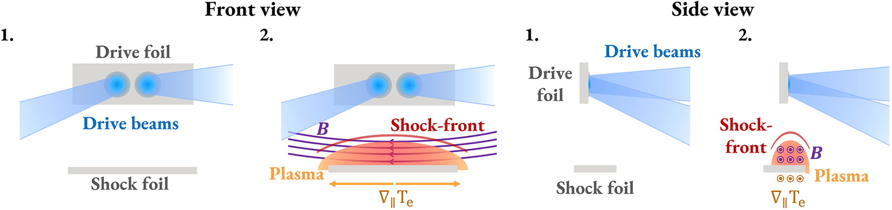
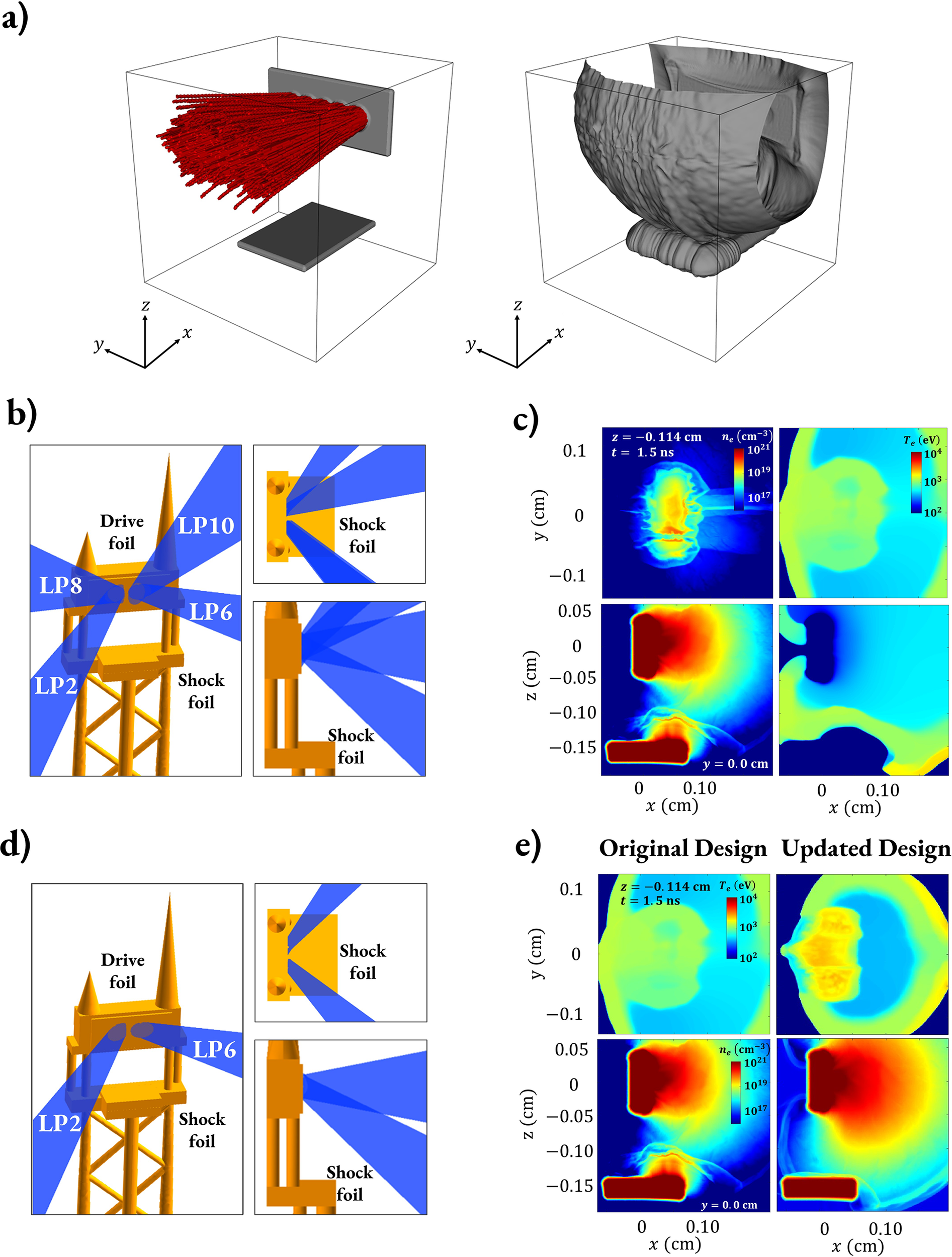


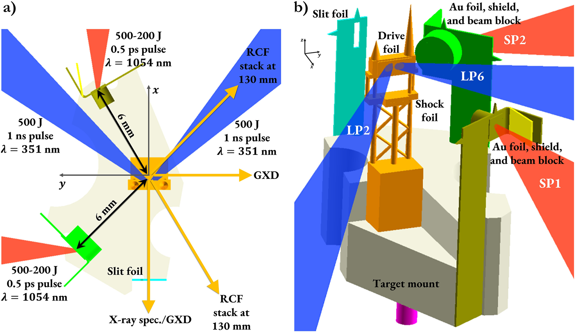
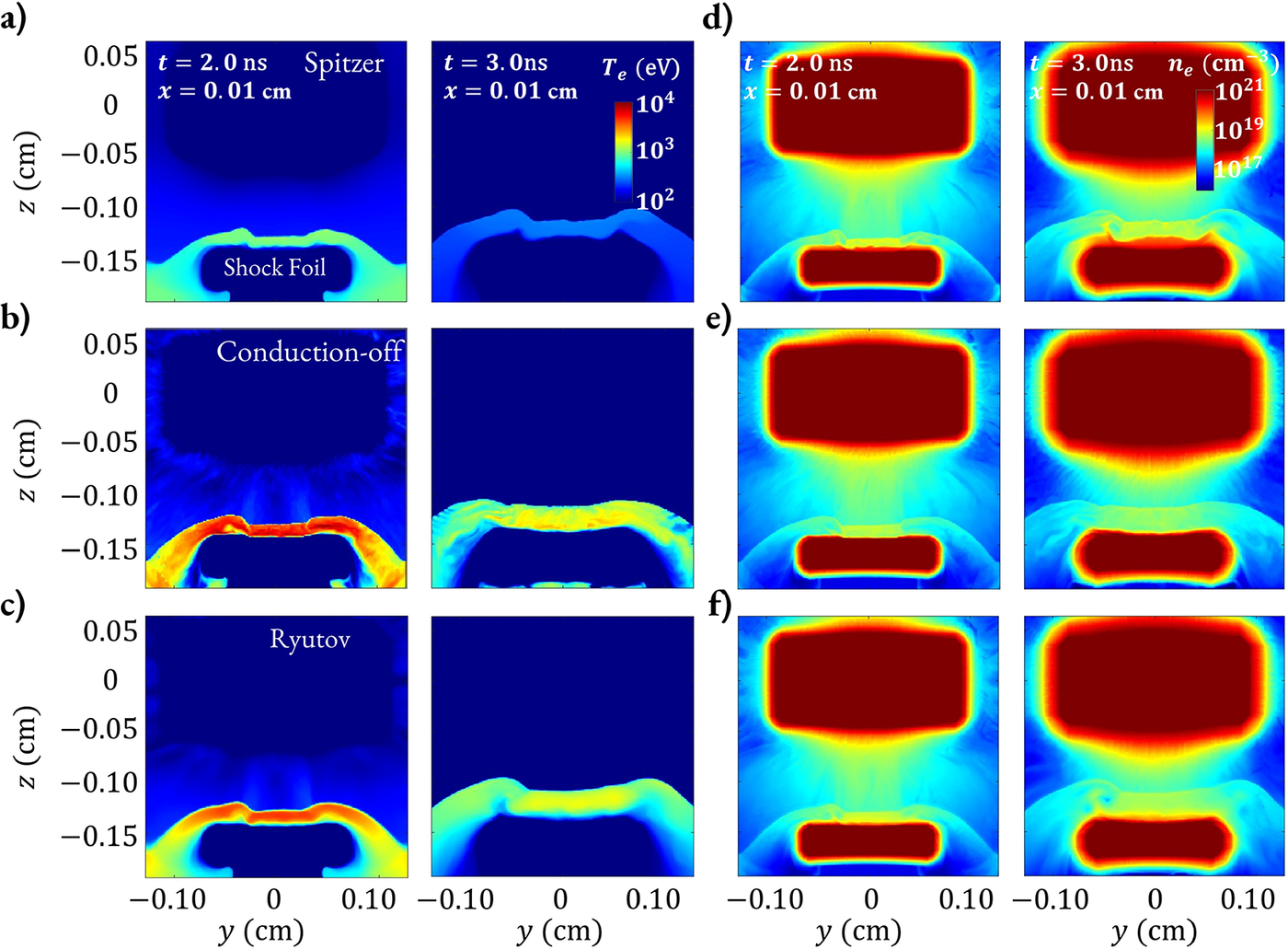


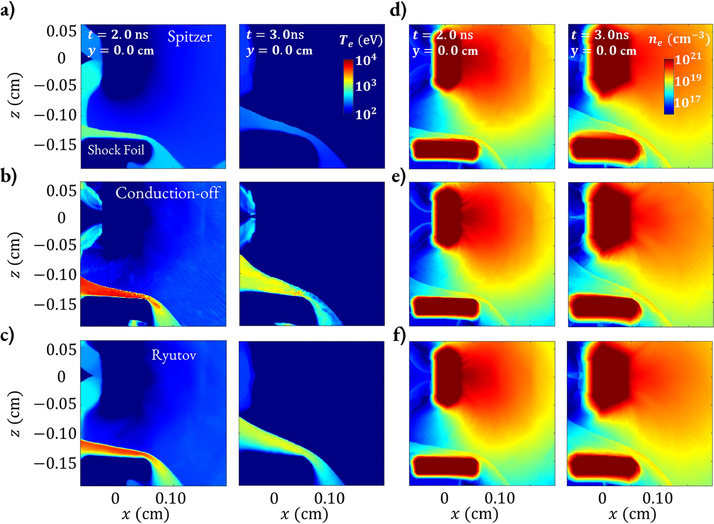


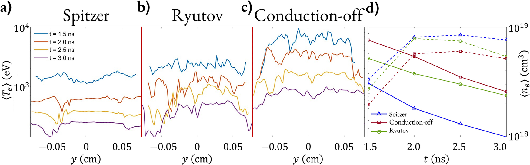


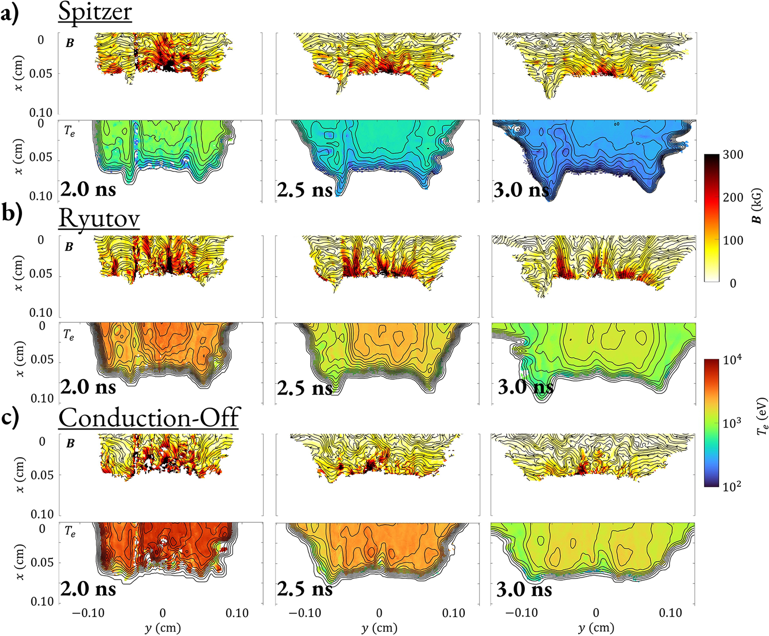


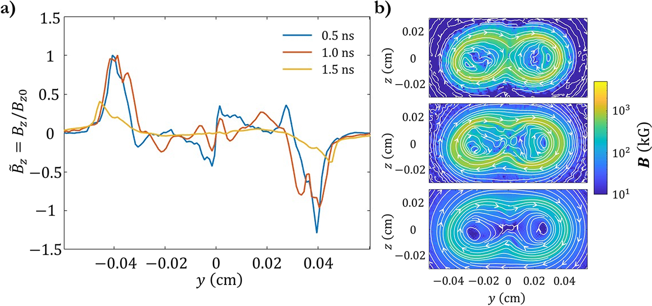


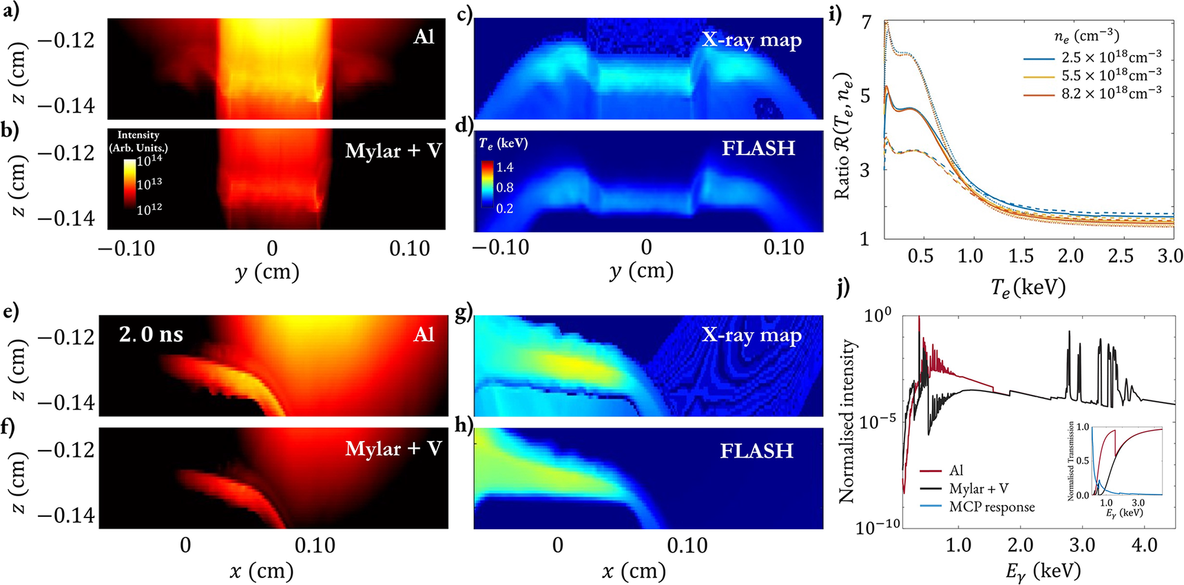


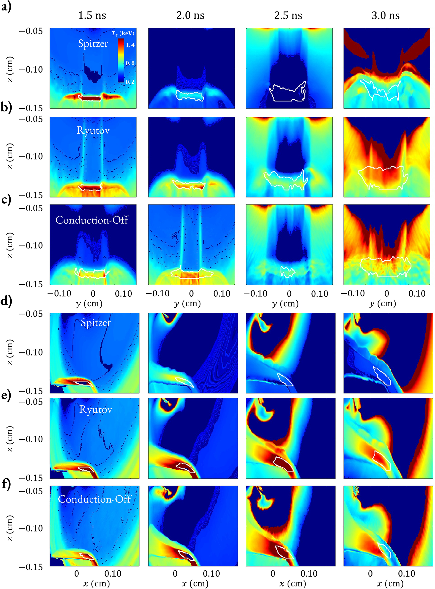


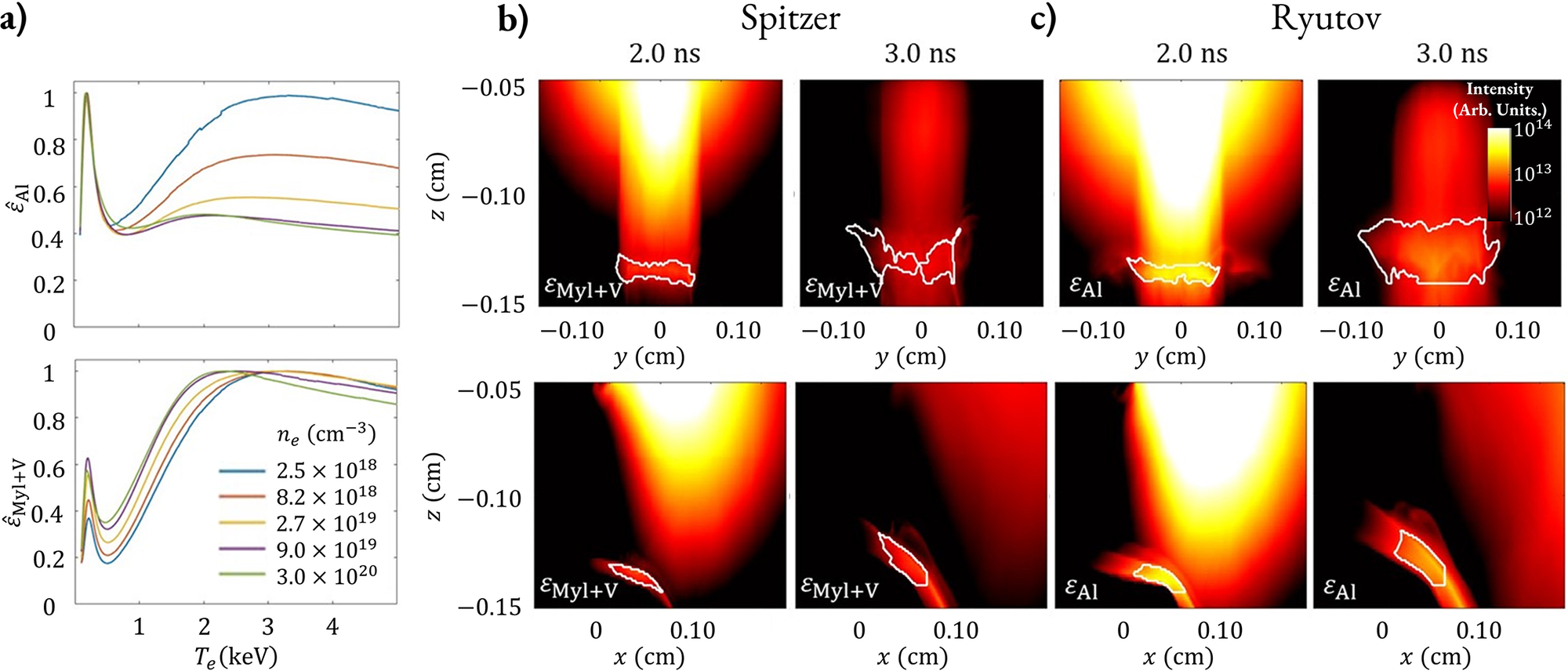


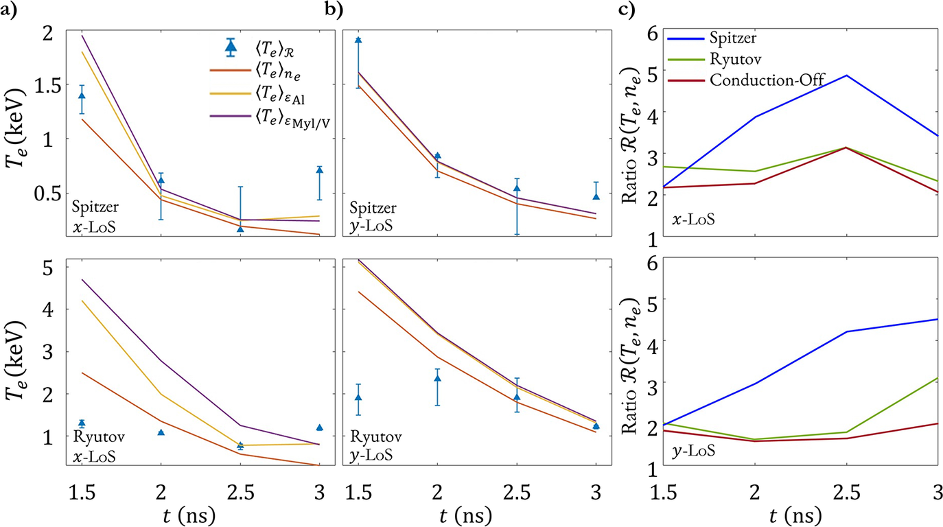


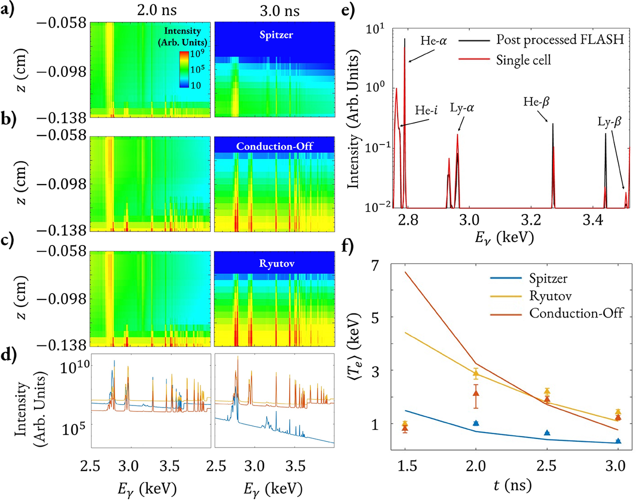


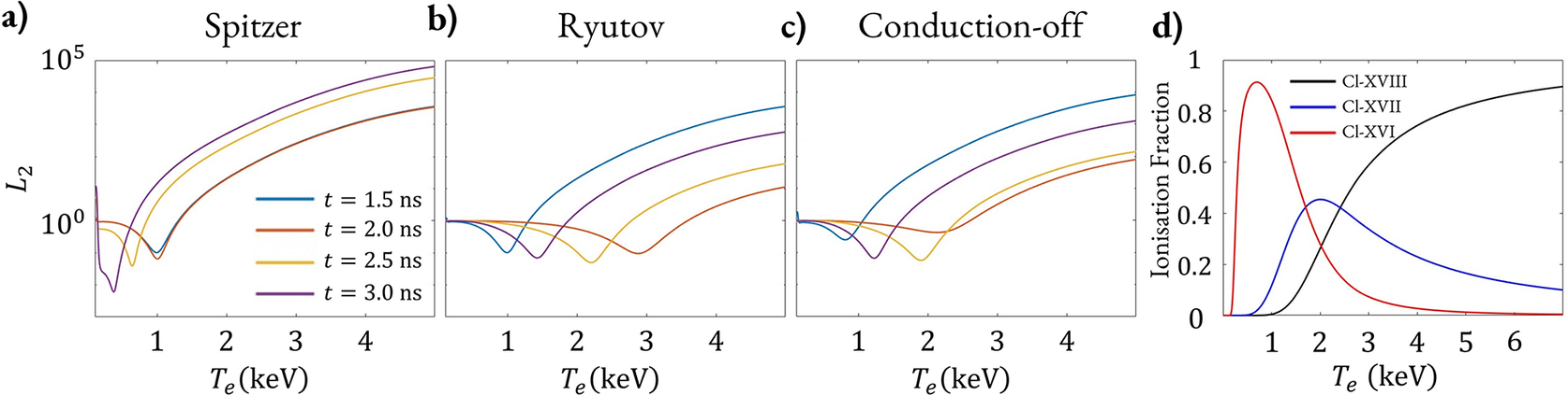


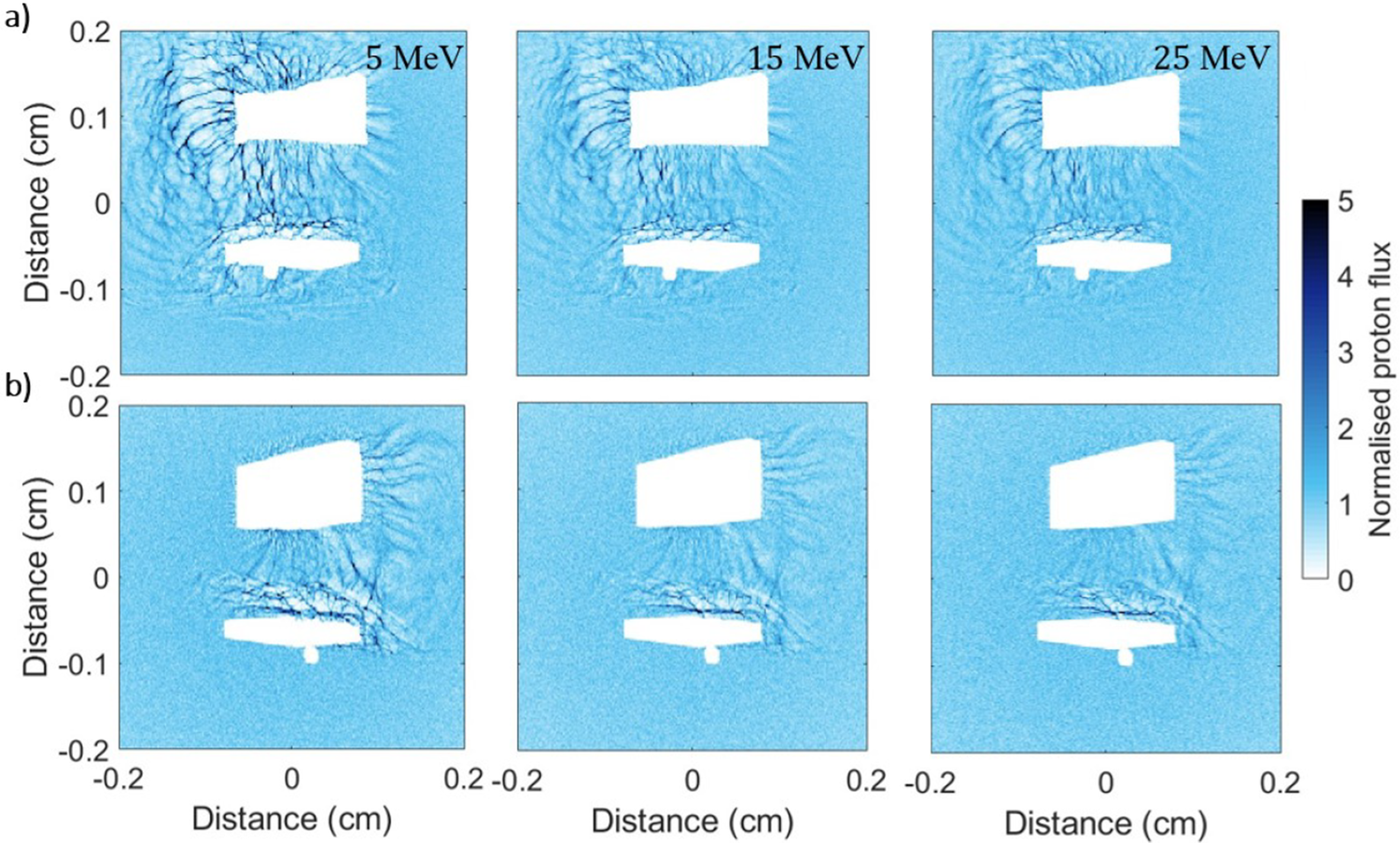


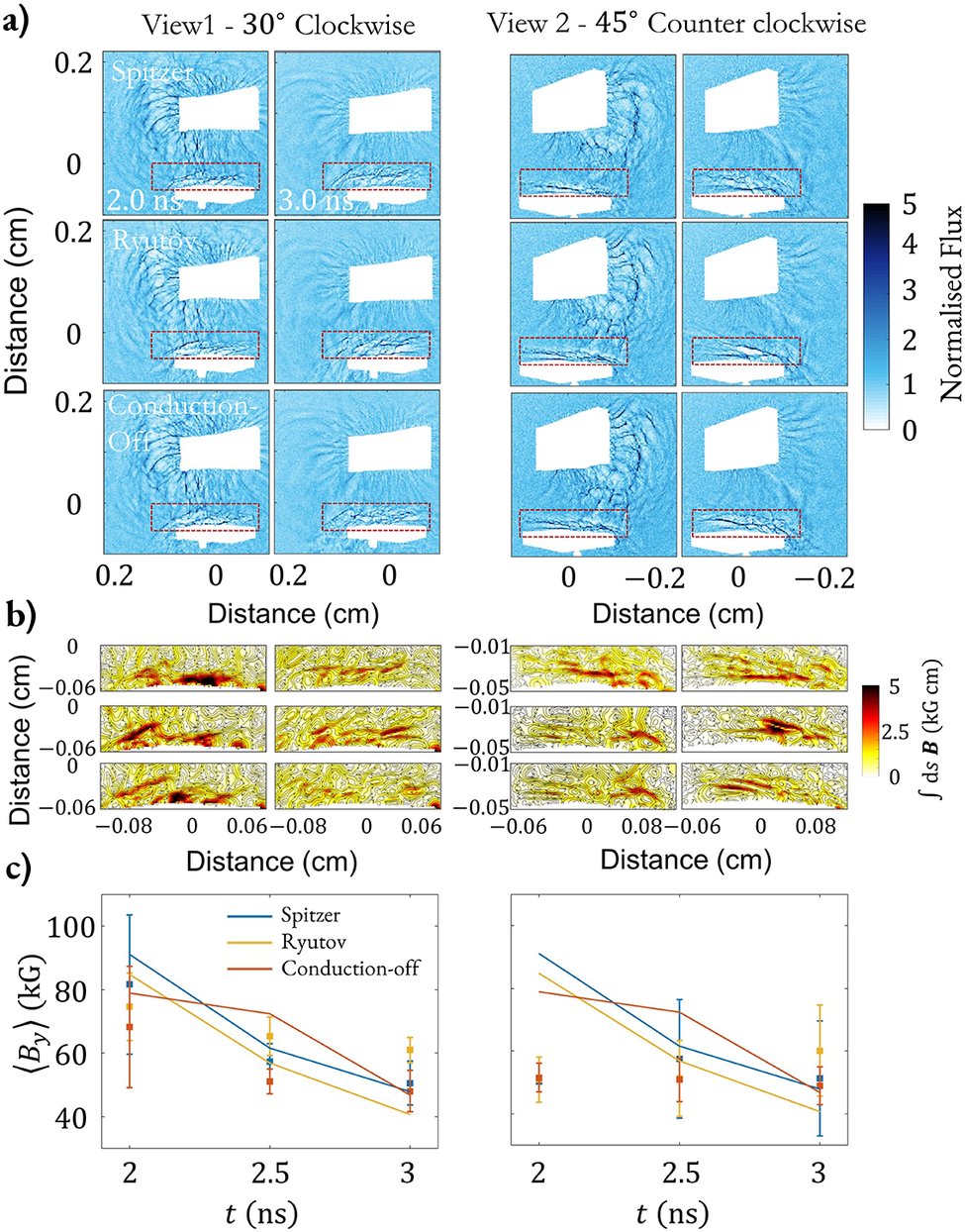

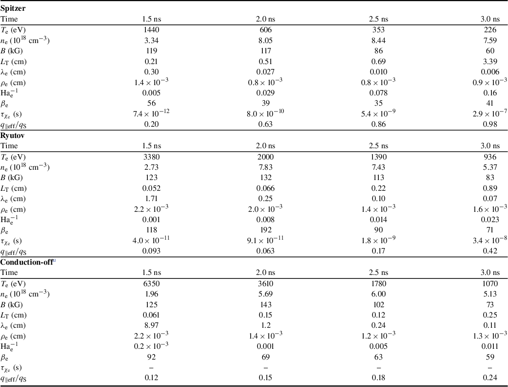

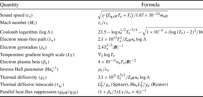


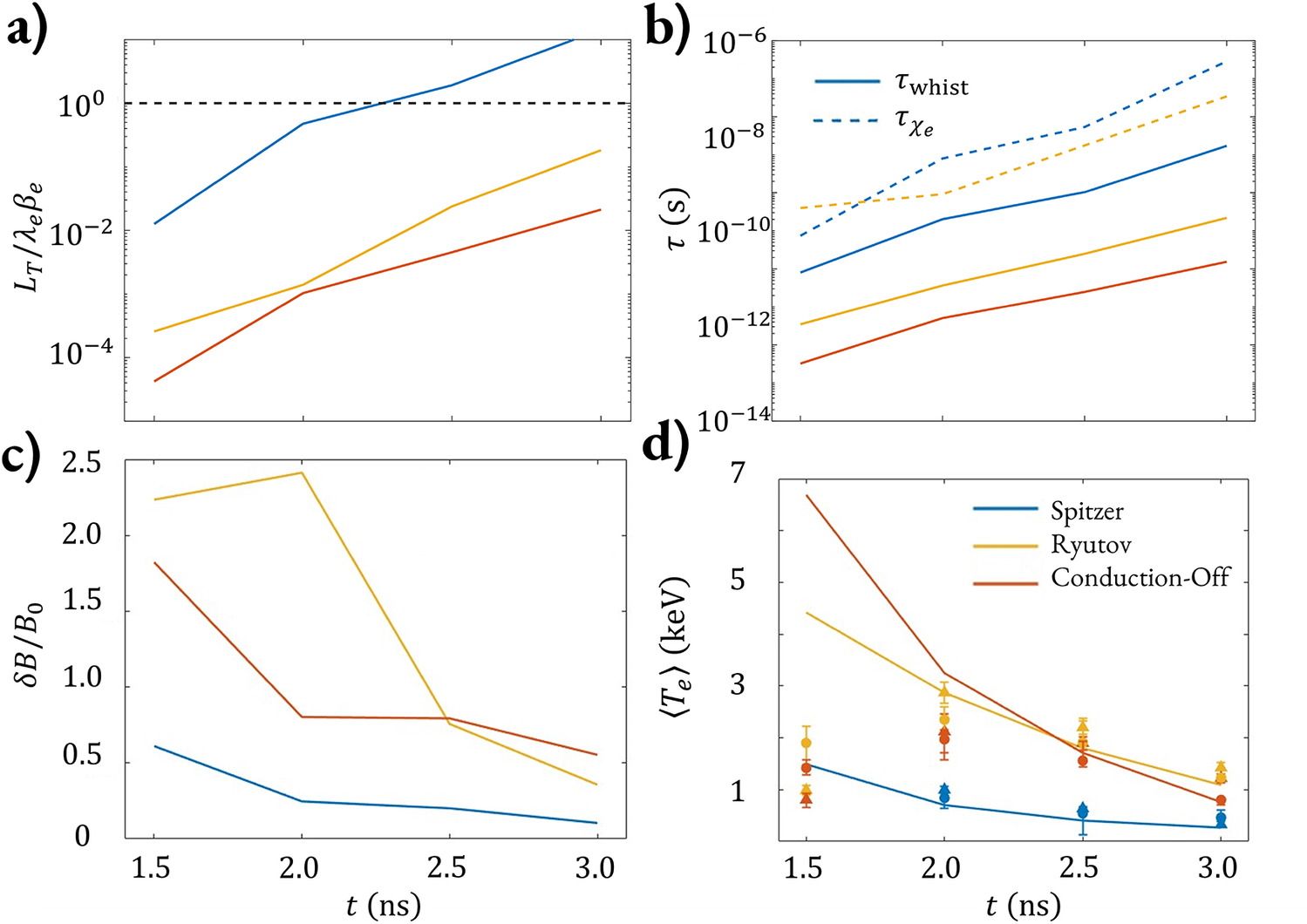


 Open access

